Spiral Arms and a Massive Dust Disk with non-Keplerian Kinematics:
Possible Evidence for Gravitational Instability in the Disk of Elias 2-27CASA (McMullin et al. 2007), eddy (Teague 2019), bettermoments (Teague & Foreman-Mackey 2019), PHANTOM (Price et al. 2018), mcfost (Pinte et al. 2006; Pinte et al. 2009), galario (Tazzari et al. 2018), frankenstein (Jennings et al. 2020), Astropy (Astropy Collaboration et al. 2013; Astropy Collaboration et al. 2018),
Matplotlib (Hunter 2007), emcee (Foreman-Mackey et al. 2013)
Abstract
To determine the origin of the spiral structure observed in the dust continuum emission of Elias 2-27 we analyze multi-wavelength continuum ALMA data with a resolution of 0.2 arcsec (23 au) at 0.89, 1.3 and 3.3 mm. We also study the kinematics of the disk with 13CO and C18O ALMA observations in the 3-2 transition. The spiral arm morphology is recovered at all wavelengths in the dust continuum observations, where we measure contrast and spectral index variations along the spiral arms and detect subtle dust-trapping signatures. We determine that the emission from the midplane is cold and interpret the optical depth results as signatures of a higher disk mass than previous constraints. From the gas data, we search for deviations from Keplerian motion and trace the morphology of the emitting surfaces and the velocity profiles. We find an azimuthally varying emission layer height in the system, large-scale emission surrounding the disk, and strong perturbations in the channel maps, co-located with the spirals. Additionally, we develop multigrain dust and gas SPH simulations of a gravitationally unstable disk and compare them to the observations. Given the large scale emission and highly perturbed gas structure, together with the comparison of continuum observations to theoretical predictions, we propose infall-triggered gravitational instabilities as origin for the observed spiral structure.
I Introduction
Protoplanetary disks around young stars have shown various structures in their thermal dust continuum emission. Observing and understanding their origin is necessary to understanding the chemical, physical and dynamical processes that are ongoing in a protoplanetary disk. Of the structures present in dust emission, rings and gaps are the most common (ALMA Partnership et al. 2015; Andrews et al. 2018; Huang et al. 2018a; Long et al. 2018; Fedele et al. 2018, e.g., ), albeit arcs and spirals have also been observed in some systems (Dong et al. 2018; Huang et al. 2018b, e.g., ).
Observing with instruments such as the Atacama Large Millimeter/submillimeter Array (ALMA) is crucial to our understanding of planet-formation mechanisms, as we can observe at wavelengths that trace continuum emission from the cold midplane (Testi et al. 2014, e.g.,), where we expect planets to be forming or have already formed. In the case of midplane spiral structures, their origin may be linked to the presence of a companion; stellar, fly-by or planetary (Pohl et al. 2015; Forgan et al. 2018b; Cuello et al. 2019; Bae & Zhu 2018a; Dong et al. 2018; Keppler et al. 2020). Spirals may also be excited if the system is gravitationally unstable. Gravitationally instability is expected in cool and massive disks, where the disk-to-star mass ratio is larger than 0.1 (Bell et al. 1997; Gammie 2001; Lodato & Rice 2004; Kratter & Lodato 2016; Hall et al. 2016; Rice 2016; Zhang & Zhu 2020; Hall et al. 2019; Cossins et al. 2009). To date, not many spirals in dust continuum emission have a clear origin, except for those in multiple systems where the presence of spirals has been linked to stellar interactions (Kurtovic et al. 2018; Rosotti et al. 2020). On the other hand, there are disks were spirals have been reported at millimeter wavelengths and where no companion to which the spiral origin may be linked to has been detected yet (Pérez et al. 2016; Huang et al. 2018b; Dong et al. 2018, to date these are Elias 27, IM Lup, WaOph 6, and MWC 758, ). If no companion is detected and the disk is massive compared to the host star mass, the gravitational instability (GI) scenario arises as a possible explanation for the origin of the observed spirals. Studying disks undergoing GI is important, as population synthesis models show that GI primarily ends up forming brown dwarf mass objects (Forgan et al. 2018a; Hall et al. 2017). It seems that giant planet formation through GI is rare (Rice et al. 2015), but it may still be the formation mechanism for important systems like HR 8799 (Vigan et al. 2017).
Elias 2-27 is a young (0.8 Myr) M0 star (Andrews et al. 2009) located at a distance of 116 pc (Gaia Collaboration et al. 2018) in the Oph star-forming region (Luhman & Rieke 1999). It harbors an unusually massive protoplanetary disk, the disk-to-star mass ratio of Elias 2-27 is reported to be 0.3 (Andrews et al. 2009; Pérez et al. 2016). The initial detection of two large-scale spiral arms was obtained with medium-resolution ALMA observations by Pérez et al. 2016. Due to the brightness and accessibility of the source, it became one of the Disk Substructures at High Angular Resolution Project (Andrews et al. 2018, DSHARP,) targets, allowing further analysis of the dust emission at high resolution. Its distinctive morphology consists of two extended quasi-symmetric spiral arms and a gap, 14 au wide, located at 69 au from the star (Huang et al. 2018a; Huang et al. 2018b). Due to its characteristic structure, the system has been the subject of several theoretical studies, concluding that GI is a possible origin to the spiral arms (Hall et al. 2018; Forgan et al. 2018b; Meru et al. 2017; Bae & Zhu 2018b). Though GI seems to explain the spiral morphology, it does not explain the dust gap, which could be carved by a companion of 0.1 MJ as constrained in hydrodynamical simulations by Zhang et al. 2018. Localized deviations from Keplerian motions at the location of this dust gap have been recently found, strengthening the hypothesis of a planetary-mass companion in the gap (Pinte et al. 2020). However, a lower mass inner companion, such as the one proposed to open the gap, would not be able to excite the observed spiral arms (Meru et al. 2017).
Overall, Elias 2-27 appears to be a strong candidate to be a gravitationally unstable protoplanetary disk, but there are many tests to be done in order to determine if this is in fact the origin of the observed spirals. GI spirals will create pressure enhancements where we expect solids to be trapped and grain-growth favored (Rice et al. 2004; Rice et al. 2005; Dipierro et al. 2015). This will not occur in the case of a companion, as companion-induced spirals will co-rotate with the planet at its Keplerian speed, faster than the background gas flow at their location, prohibiting dust growth and accumulation (Juhász et al. 2015). Another morphological signature is the expected symmetry of the spirals produced by GI, which should have a constant pitch angle in a logarithmic spiral model (Forgan et al. 2018b). Thus, measurements of dust growth signatures together with symmetric, constant pitch angle, logarithmic spirals, in a protoplanetary disk point towards a GI scenario.
Additionally, valuable dynamical information may be obtained from gas observations. The presence of planets or companions leaves distinct footprints in the kinematics and these perturbations may be constrained by the amplitude of the gas deviations from the expected Keplerian motion of an unperturbed disk. The current state-of-the art methods vary from tracing pressure gradients (Teague et al. 2018), observing deviations from expected isovelocity curves in the channel maps (’kinks’) (Pinte et al. 2019; Pinte et al. 2018a; Pinte et al. 2020; Perez et al. 2015) and using the mean velocity maps to model the velocity structure of the disk and detect Doppler flips in the residuals (Pérez et al. 2020; Pérez et al. 2018b). For GI spirals, Hall et al. 2020 characterizes the presence of a “GI-wiggle” that, contrary to companion-disk interactions, will not be spatially localized but rather be a large scale perturbation, present throughout a wider velocity range, co-located with the spirals. Analyzing the disk kinematics complements the analysis of the observed dust structures and allows us to understand and connect the various ongoing processes.
Previously published gas observations of Elias 2-27 in the 12CO and 13CO in J=2-1 transition show heavy absorption, as the star is quite embedded in its cloud (Andrews et al. 2009; Pérez et al. 2016; Andrews et al. 2018; Pinte et al. 2020). In this study we present 13CO and C18O observations in J=3-2 transition. The higher energy transition and lower abundance of the isotopologues allows us to avoid some of the cloud contamination, while also probing closer to the midplane than previous works.
The present paper offers new observational constraints on Elias 2-27 and is organized as follows. Section 2 provides an overview on the calibration and imaging process of the observations, section 3 analyzes the spirals in the multi-wavelength continuum data, section 4 studies the 13CO and C18O emission, through a geometrical analysis of the moment maps and the localization of perturbations in channel maps, section 5 shows the analysis of hydrodynamical simulations computed for a GI disk using the derived observational parameters of Elias 2-27, section 6 discusses the results and determines the possible origin of the spirals, and finally, section 7 summarizes the main findings of this work.
II Observations
We present multi-wavelength (Band 3, 6 and 7) dust continuum and spectral line (13CO and C18O ) ALMA data of Elias 2-27. In the case of the Band 6 (1.3 mm) observations, the imaged data corresponds to the one presented in Pérez et al. 2016, detailed information regarding the calibration of this dataset may be found in the original publication. For the Band 7 (0.89 mm) and Band 3 (3.3 mm) observations, the dust continuum data was first calibrated through the ALMA pipeline and afterwards, phase and amplitude self-calibration was applied. Additionally, following the calibration procedure described in Andrews et al. 2018, we applied astrometric and flux scale alignment, to correct for spatial offsets between the center of emission of different observations and relative flux scale differences. In both bands we have short (15 m-313.7 m in Band 7, 15.1 m-2.5 km in Band 3) and long (15.1 m-1.4 km in Band 7, 21 m-3.6 km in Band 3) baseline observations, in order to account for all of the emission from different spatial scales of the disk. Spatial offsets are corrected by locating the center of emission through a Gaussian fit in the image plane of each observation and adjusting phase and pointing centers with the Common Astronomy Software Applications (McMullin et al. 2007, CASA) tasks fixvis and fixplanets respectively. The absolute flux calibration uncertainty of ALMA data is expected to be 10, and we note that after self-calibration the relative flux scales are consistent within 5 for different observations in the same band. To adjust these amplitude scale differences we compare the deprojected, azimuthally averaged, visibility profiles and scale them using the short-baseline data as reference for the gaincal task, following the methodology in Andrews et al. 2018. For Band 7 data we apply the spatial offset corrections and amplitude scaling before any self calibration as relative flux scales vary between observation sets. In the Band 3 data set we have a higher flux scale difference from the initial datasets (20), probably due to atmospheric conditions as we can visually see that the image quality is not the best. Therefore, in Band 3 we conduct self-cal of the short-baseline observation and afterwards, with a flux scale difference of 3, we perform the spatial and amplitude scale corrections.
Self-calibration was first conducted on the dust continuum emission short-baseline data and the result combined with the long-baseline data to be self-calibrated all together. The selected time intervals for both phase and amplitude self-calibration start with the longest available total integration period for the initial round, and afterwards, each following time interval was half of the previous interval. The longest and shortest intervals used were, 1500s and 46s for the phase calibration of the joint 0.89 mm data, and 2860s and 178s for the phase calibration of the joint 3.3 mm data. For the calibration of the short baseline data, the time intervals of phase calibration were between 1080s and 270s for the 0.89 mm data, and 304s and 9.5s for the 3.3 mm data. In the case of the amplitude self-cal time intervals, in Band 7 only one round was required in both short baseline and joint data, so the solutions were obtained from the longest time interval. In Band 3 the short baseline data had one round of amplitude calibration and the joint data set had two rounds. Self-calibration rounds were applied until signal-to-noise ratio (SNR) improvement was less than 5 in the case of Band 7 data and until there was no SNR improvement in the case of Band 3. For the short baseline data at 0.89 mm, we conducted 3 rounds of phase calibration and 1 round of amplitude calibration. The combined dataset at 0.89 mm had 7 rounds of phase calibration and 1 round of amplitude calibration, overall the peak SNR in the joint dataset improved 300. The short baseline data at 3.3 mm had 6 rounds of phase calibration and 1 round of amplitude calibration, the joint data set had 5 rounds of phase calibration and 2 round of amplitude calibration. In the joint dataset, the SNR improvement was 6.
For the final imaging we used multi-scale tclean for all the images, using a 1 stopping threshold (where is the image RMS) for the Bands 3 and 6 data, and a 2 stopping threshold in Band 7. Robust weighting values were 1.0 in the case of Band 6, and 0.5 for Bands 3 and 7. We also set the gain value to 0.05 and cyclefactor parameter in tclean to 2.0, to have a more detailed cleaning, by substracting a smaller fraction of the source flux from the residual image and triggering a major cycle sooner. All images have comparable beam sizes: 0.220.17 beam (26 au20 au) at 0.89 mm, 0.260.22 beam (30 au26 au) at 1.3 mm, and 0.260.20 (30 au23 au) beam at 3.3 mm. At each wavelength the image RMS is approximately 93 Jy/beam, 86 Jy/beam and 10 Jy/beam, respectively for 0.89 mm, 1.3 mm and 3.3 mm.
The observations of C18O and 13CO were obtained simultaneous to the dust continuum emission in Band 7 (0.89 mm) and in the transition. C18O is observed at 329.330 GHz, with a spectral resolution of 0.035 MHz and 13CO at 330.588 GHz, with a spectral resolution of 0.121 MHz. After applying the same self-calibration solutions as to the dust continuum of Band 7, the emission was first imaged using natural weighting (robust parameter of 2.0) and not applying any uvtapering or uv-range filtering, in order to be sensitive to large-scale emission with a beamsize of 0.290.22 ( 3425 au) for 13CO and 0.300.23 ( 3527 au) for C18O (see figures in Appendix A). In order to avoid the cloud contamination present in the disk (Pérez et al. 2016; Huang et al. 2018b) we exclude large-scale emission by considering only baselines longer than 36m for 13CO (scales shorter than 6.4, 740 au) and 45m for C18O (scales shorter than 5.11, 590 au). We also applied uvtapering of 0.20.115, PA= 0∘ for 13CO and 0.20.0, PA= 0∘ for C18O, in order to obtain a roughly round beam. The final images that trace the disk emission were obtained with a robust parameter of 0.5, resulting in a beam size of 0.260.25 ( 29 au) for 13CO and 0.310.29 ( 35 au) for C18O. We imaged all channel maps in both 13CO and C18O using a 0.111 km s-1 spectral resolution, though the C18O data was observed with a finer spectral resolution (0.032 km s-1), and found the best compromise of SNR by using a broader spectral resolution.
We also recover gas emission from CN v, N in and , these additional molecules will be studied separately in future work. We do not recover any emission from requested observations of CN v, N in or SO 3 v , at the achieved sensitivity level of 3mJy/beam.
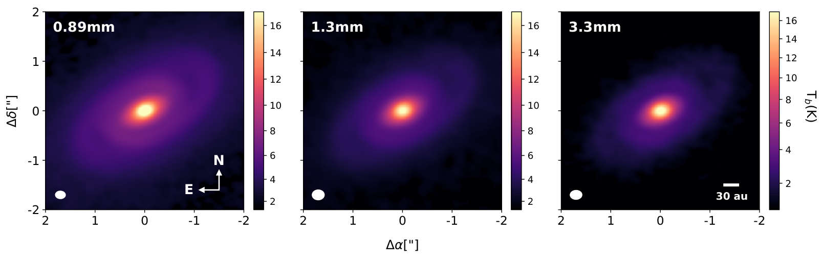
III Dust Spiral Structure
We recover the spiral structure at all wavelengths, as shown in Figure 1. Given the 25 au beam size, we are not able to fully resolve the 69 au gap but can distinguish it as a small decrease in brightness temperature at all wavelengths in Figure 1. For all calculations throughout this study, we will assume the gap location, disk inclination, and disk position angle as derived in Huang et al. 2018a, which are 69.1 au, 56.2, and 118.8, respectively.

| Wavelength | Spiral Arm | Angle Range | [au] | Pitch Angle | |
|---|---|---|---|---|---|
| 0.89 mm | NW | -251∘ to -5∘ | 249.8 | 12.9∘ | |
| SE | -70∘ to 150∘ | 111.5 | 13.9 | ||
| 1.3 mm | NW | -250∘ to -35∘ | 250.2 | 12.9 | |
| SE | -61∘ to 135∘ | 115.5 | 0.234 | 13.2 | |
| 3.3 mm | NW | -260∘ to -23∘ | 249.9 | 12.9 | |
| SE | -50∘ to 140∘ | 113.6 | 13.0 |
III.1 Tracing the Spiral Morphology
To trace the spiral structure from our dust continuum images, we radially subtract an azimuthally-averaged radial profile of the emission and trace the spiral features from these “subtracted images” (Huang et al. 2018b, as done in ). From the subtracted images, shown in the top panels of Figure 2, we find the radial location of maximum emission along each spiral, at azimuthal steps sampled every 9∘, between a determined azimuthal angle range (values in Table 1). The radial extent where we trace the maxima of emission is determined visually. To aid our visual criteria we consider radial locations no further than where we have a signal of 5 times the RMS in the non-subtracted image.
Previous analyses of Elias 2-27 (Pérez et al. 2016; Huang et al. 2018b) have shown that a logarithmic spiral model, with a constant pitch angle, can adequately trace the spiral morphology. Therefore, we use MCMC modelling to find the best-fit parameters for a logarithmic spiral model, considering the location data of each spiral and each observed wavelength. The spiral form is given by:
| (1) |
Here is the polar angle in radians measured from the North and to the East (left), for reference see coordinates in Figure 1. are free parameters, with the radius at , measured in au, and relates to the pitch angle of the spiral arms (), as . The uncertainty on the location of each measured maxima is assumed to be the astrometric error11 1 see Sect. 10.6.6 in https://almascience.nrao.edu/documents-and-tools/cycle5/alma-technical-handbook/view for further details.: , were is the approximate position uncertainty of a feature in milliarcseconds, is the peak/RMS intensity ratio of the data point on the image, is the observing frequency in GHz and is the maximum baseline length in kilometers.
The top panel of Figure 2 shows the maxima along each spiral from the subtracted images. In the middle panels are the deprojected radial locations of each maxima, measured from the center, as a function of azimuthal angle. Grey lines show logarithmic spiral models, derived from 300 draws of the posterior values after convergence of the MCMC simulations for the best-fit parameters of each spiral arm. The horizontal line at 148 au marks the location where we observe a break in the spiral arm, at all wavelengths, clearest in the South-East spiral, also subtly present in the North-West spiral. Huang et al. 2018b had previously noted a possible decrease in the pitch angle value outside R 150 au. The bottom panel (Figure 2) shows the polar deprojection of the subtracted data, with a vertical line marking the dust gap location. The red/blue lines show the best-fit model for the logarithmic spirals. The median value for the parameters of the logarithmic spiral model, for each spiral and wavelength, are shown in Table 1, along with the 16th and 84th percentile uncertainties derived from the posteriors.
We note that the pitch angle values retrieved here, 12.9∘ and 13.3∘, for NW and SE spiral respectively (similar between wavelengths, see Table 1), are different than the recovered pitch angles from Huang et al. 2018b (15.7∘ and 16.4∘, for NW and SE spiral). When applying our method to the high-resolution dataset presented in Huang et al. 2018b, we retrieve the same results as in their work. The pitch angle difference between this work and theirs is probably due to beam smearing effects, combined with the challenge of image subtraction in lower-resolution data (Huang et al. 2018b, as discussed in), as the angular resolution difference between datasets is a factor of 4-5.
III.2 Contrast variations along the spirals

We test the contrast at comparable locations over different wavelengths, for this may provide evidence of dust trapping. If indeed there is dust growth within the spiral arm or large particles are trapped at this location, then at longer wavelengths we could expect to observe higher contrast. The latter effect is due to larger particles being more densely packed in the spiral arm (Rice et al. 2004), this has been shown to occur in the case of dust-trapping vortex studies (Cazzoletti et al. 2018). We compute how the contrast varies radially along each spiral arm, with respect to a fixed “inter-arm” region, which is expected to be a location where we can be sure there is no emission from the spiral arms. Considering the symmetry between the spirals, the inter-arm region of each spiral is assumed to follow the same shape of the corresponding spiral arm, but rotated by 90 degrees clockwise from the spiral location. The top panels of Figure 3 show a polar projection of the dust continuum, overlayed are the best-fit model of the spirals for each wavelength in continuous line and this same model, shifted 90 degrees clockwise, tracing the inter-arm region, in dashes. From this figure it is clear that the interarm region effectively traces zones of lower emission, compared to the spiral arm location.
The contrast is calculated, from the original images, as the ratio between the emission at the spiral and the inter-arm regions, at each radius and for both spiral arms. We use the previously derived parameters and calculate the contrast along the best-fit spiral model for each wavelength, binning the data azimuthally every 15∘. The standard deviation within the bin is used as the error of each averaged flux measurement, both for the interarm and spiral region. The contrast curves for each wavelength are shown in the bottom panels of Figure 3. The NW spiral remains the strongest spiral at all wavelengths with an average contrast value 25-33 higher than the SE spiral. Both spirals maintain a similar contrast throughout their radial extent, deviating in the 0.89 mm and 1.3 mm observations only 11 from the average contrast value in the case of the SE spiral and 17 in the case of the NW spiral. In the 3.3 mm data the contrast variation increases and deviations from the average value increase to 16 in the SE spiral and 24 in the NW. For the 0.89 mm, 1.3 mm and 3.3 mm emission, the radial distance of the maximum contrast value is, respectively for (NW, SE) spirals, (125 au, 117 au), (129 au, 127 au) and (129 au, 126 au). For the minimum contrast location, in the same order, the radial distances are (155 au, 149 au), (161 au, 147 au) and (150 au, 142 au). We observe in our contrast curves that the radial location of the maximum contrast slightly shifts outwards with wavelength, no global shifts are detected in the minimum contrast distances, however the minimum contrast of the SE spiral appears to shift inwards at longer wavelength. Overall our values are in agreement with previous measurements of Huang et al. 2018b where the peak contrast is located at 123 au and low contrast at 147 au (measured from higher angular resolution 1.3 mm data). While the form of the contrast curve in the 1.3 mm emission agrees also with the previous studies (Pérez et al. 2016; Huang et al. 2018b), at larger radial distances we observe a decrease in the contrast of both spirals in the 0.89 mm emission and also in the SE spiral in 3.3 mm, contrary to the apparent growing contrast at larger radial distance observed in the 1.3 mm emission.
If we follow the peak contrast of both spirals, located at 125 au, we see a slight variation in the contrast value, which grows larger with longer wavelength. The peak contrast value of the NW spiral increases by 11 from the 0.89 mm to the 1.3 mm emission and by 8 between the 1.3 mm and 3.3 mm emission. The SE spiral increases its peak contrast value 5 initially and in the 3.3 mm data decreases the peak contrast by 2 with respect to the 1.3 mm emission. Minimum contrast values also shift, but do not show any correlation with varying wavelength. We note that previous studies on this source measured the contrast differently, using the ratio between the spiral flux and the minimum flux at the same radial location (Huang et al. 2018b; Pérez et al. 2016). For completeness, we test our results using the minimum flux method used in the previous studies, and obtain similar contrast curves in which we also measure increasing peak contrast values towards longer wavelengths. However, we do not consider these results, for the minimum flux at a determined radial distance is found at different azimuthal angles between different wavelengths. Therefore, the contrast calculated using the minimum radial flux does not sample comparable locations between different wavelengths, something necessary in order to detect possible signatures of dust growth at a given location, which we achieve by using the interarm region.
III.3 Spectral Index Analysis

The presence of dust growth throughout the disk can be inferred using the multi-wavelength continuum observations to compute the disk spectral index. The spectral index () of the spectral energy distribution follows , where corresponds to the measured intensity, from the image plane, at frequency . In the optically thin regime, if has values between 2-2.5 it can be an indicator towards the presence of large, up to cm-sized, grains and hence dust growth at the location of such values (Kwon et al. 2009; Testi et al. 2014; Pinilla et al. 2017; Cazzoletti et al. 2018; Macías et al. 2019, e.g., ). To adequately compare the emissions from all three wavelengths, the calculations in this section are done from dust images at equal resolution and centered in the peak brightness. We use the task imsmooth in CASA to especify a round, 0.260.26 beam (31 au). Figure 4 shows in the top panel the azimuthally averaged brightness temperature of the smoothed, equal resolution images.
We calculate as the best-fit slope of a linear model applied to the logarithmic space ( ln ln), using all wavelengths available in this study. From an MCMC fit we obtain a posterior distribution of , with best-fit and uncertainties computed from the 50th, 16th, and 84th percentile values. From the azimuthally averaged intensity profiles, we compute an radial profile shown in the middle panel of Figure 4. We retrieve a disk average value of 2.60.06, with in the inner 50 au. These low values in the inner disk will be discussed in section 5.1 and are probably related to optically thick emission where self-scattering at long wavelengths is a relevant process.
We apply the same techniques described in Huang et al. 2018a to calculate the optical depth at our various wavelengths. The main assumption relies on approximating the midplane temperature profile (), assuming a passively heated, flared disk in radiative equilibrium (Chiang & Goldreich 1997, e.g.,) and considering that the millimeter emission follows this temperature profile, if it traces the midplane. From the temperature profile, we compute the expected blackbody emission (), using Planck’s law, and relate it to the measured intensity () through , following . will depend on the assumed flaring of the disk and the stellar luminosity (Andrews et al. 2018, we use the DSHARP values for flaring and stellar luminosity of = 0.02 and = -0.04 0.23,).
The computed optical depth profiles are shown in the bottom panel of Figure 4. We note that at 0.89 mm the modeled is 2 times larger than the measured . In Rayleigh-Jeans regime, as expected for mm emission, exp. Then, if is overestimated it will produce lower optical depth values and the emission will appear more optically thin than it really is. The disk could be colder, or with a lower flaring value, and the emission at all wavelengths would be more optically thick. These issues will be discussed in section 5.1.
The spectral index map for Elias 2-27 and the uncertainty on the spectral index are presented in Figure 5. We only consider emission above 5 at all wavelengths for this calculation, and we adopt the rms of each image as the uncertainty on the intensity for each pixel. The best-fit spiral model from the 0.89 mm dust emission is overlaid for reference, along with the dust gap location (69 au). Contour lines for values of [2.0, 2.25, 2.4] and for uncertainties at the level of [0.01, 0.025, 0.05, 0.1] are presented. We observe that contours tracing 2.4 seem to be coherent with the spiral morphology as traced by the best-fit spiral. This is specially apparent in the NW spiral location. The variations between the spiral and inter-arm region at the NW spiral location are , with uncertainties of . Overall, we observe lower co-located with the spiral features. At the gap location no particular behaviour is observed, except for a decrease in values inwards from the gap location. As noticed in the radial profile, in the inner disk (50 au) reaches values below 2.0.

Another indicator of dust growth is that smaller grains, traced by shorter wavelengths, will be less concentrated than larger grains observed at longer wavelengths. This will translate into a width difference along the dust-trapping structure, such that smaller grains will be more widely spread than larger grains within a dust-trap. Such behaviour has been constrained in different sources with vortex-like structures, likely tracing dust traps (Casassus et al. 2015; van der Marel et al. 2015; Cazzoletti et al. 2018; Casassus et al. 2019). The measurement of the width variation cannot be done using a subtracted image or an azimuthally averaged profile, both options would introduce artifacts or remove relevant emission, therefore, we must use the original image. We decide to trace variations along a single azimuthal cut, choosing the angle were the highest spiral contrast is observed, which is located at 125 au corresponding to 224∘.
Figure 6 shows the brightness temperature profiles along the azimuthal angle of maximum spiral contrast (224∘) for all three wavelengths, the spirals can be localized as a bump in the intensity curve between 100 au-150 au in the top panel. From this it can be seen that the shape of the intensity curve is similar at all three wavelengths, with no noticeable width differences. The bottom panel shows the spectral index distribution along the azimuthal cut, calculated directly from the top panel intensity profile, as previously done for the spectral index map. In this profile we see that the East side (negative radial distance) shows a small decrease in the spectral index value at the spiral location, while the West spiral does not show significant variations. The spatial extent of the variation in the East is resolved by our beam size (0.26, 31 au).
IV 13CO and C18O emission analysis

We analyze the emission from the two observed CO isotopologues in three different ways, by: 1) studying the presence of structures in the integrated emission and in channel maps, including large-scale emission in the entire field-of-view (FOV), 2) searching for velocity perturbations in channel and velocity maps, 3) constraining the vertical height of the 13CO and C18O emitting layer, and analyzing the kinematics of these isotopologues.
IV.1 Channel and moment maps

The channel maps for both 13CO and C18O are shown in Appendix A. The known cloud absorption (Pérez et al. 2016; Huang et al. 2018b) affects the East side of the disk and blocks all 13CO emission from km s-1, while for C18O some cloud absorption is present near km s-1. We note that the South part of the disk is the brightest. The systemic velocity is determined to be 1.95 km s-1 based on the C18O channel map analysis using a spectral resolution of 0.05 km s-1 and kinematic modelling done with the eddy package (Teague 2019).
Considering all spatial scales and imaging the whole FOV, extended, large-scale emission appears in both isotopologues around Elias 2-27 (see Figures in Appendix A). As 13CO is the most abundant isotopologue, the large-scale emission appears more strongly and along a wider range of velocities than in C18O. The extended emission is clearly identified between km s-1 for 13CO, and between km s-1 for C18O. This large-scale emission appears to have a striping pattern, probably due to the lack of compact baselines in the observations. The shortest baseline is 15m, which projected in the sky for the observed frequencies recovers emission from 15 scales, however, the detected emission may extend beyond our 20 FOV. We compute integrated emission and mean velocity maps, shown in Figure 7, from the channel maps that consider the whole FOV, including emission above 3. While in 13CO the large-scale emission is seen through the entire FOV, the C18O large-scale emission is more constrained and crossing only through the East side of the disk. There is no clear velocity gradient between the large-scale emission and the disk in either isotopologue.
From here on, we focus on the channel maps that trace the material closer to the disk rather than large-scale emission. These channel maps were obtained using uv-tapering and filtering of the short baselines as described in section 2. Figure 8 shows the integrated emission (moment 0) of both CO molecules. Foreground absorption in 13CO is clear in the East side of the disk. Overlaying the continuum contours for the 0.89 mm emission and measuring along the major axis, the East side of the disk appears to have a larger extent than the West side in the gas. Figure 8 shows that the size difference is roughly 0.5” between East and West sides of the disk, in both CO tracers. At the source distance, this size difference corresponds to 58 au between the projected emission extent of each side. To measure the East/West size variations, we trace the edge of the emission in the C18O moment 0 map. The border of the disk is considered as the radius that encompasses 98 of the integrated emission at each sampled azimuthal angle (green points on the top panel of Figure 9). We define the center based on the emission peak from the Band 7 continuum data and deproject accordingly, assuming the inclination and position angle of the dust continuum. The deprojected radial distance as a function of azimuthal angle is shown in the middle panel of Figure 9. Errors correspond to the astrometric error, calculated as described in section 3.1. The edge of the disk is not well described by a circle or an ellipse; it shows two local maxima and two local minima. The global minimum distance is located along the major axis on the West, but the global maximum distance is shifted with respect to the East major axis. The locations of maximum and minimum border extents are not colocated with the continuum spiral features, or their extension.
Another feature in the moment 0 map is the presence of a “gap” of emission at large disk radii in C18O. To estimate its location, we trace the radial positions of emission minima sampling every 9∘, between 185-300 au (this range is determined by analysis of the intensity profile). Using the mean value and standard deviation of the minima radial locations (yellow points in top panel of Figure 9), we estimate the gap position at 241 24 au. In the 13CO integrated intensity map we do not observe a gap and cannot infer one from the intensity profile, even when excluding the azimuthal angles 65∘-155∘, where foreground absorption is strongest. If we trace the emission border of 13CO following the 98 integrated emission criteria, we obtain a similar emission border curve to the C18O, shown in Appendix A.
IV.2 Tracing the emitting layer in 13CO and C18O
Using the method detailed in Pinte et al. 2018b we recover the emission surface of each molecule. This is done by tracing the maxima from the upper layer of emission in the channel maps and applying geometrical relationships. The emitting layer is assumed to have a cone-like structure, this means that the height of the emitting layer should be symmetric with respect to the disk’s major axis.
If the variations in the projected radial extent of the disk found in Section 4.1 are related to variations in the emitting surface height then we would only expect symmetry along the disk’s semi-major axis in the West side of the disk. The latter can be determined from Figure 9, where we see that at the West Major Axis location () the radial distance of the emission border grows similarly when we move towards North (positive angles) or South (negative angles). This similarity in the radial distance increment maintains for in each direction (North and South), which corresponds to the complete West side of the disk. On the other hand, at the location of the East Major axis, we do not see this symmetry in the growth or decline of the radial distances towards North or South. The possible lack of symmetry is an important caveat and we expect this to affect mostly on the constraints obtained for the East side of the disk (where the variations in disk extension are larger). The emission surface we measure should be taken as a rough estimate. Details on the geometry relations can be found in the original publication (Pinte et al. 2018b).
From all available channels, we visually select those in which the top layer of gas emission can be clearly identified. For C18O we select channels at velocities 0.77 to 1.55 km s-1 and 2.44 to 3.21 km s-1. For 13CO we select channels 0.66 to 1.66 km s-1 and 2.33 to 2.77 km s-1.
The recovered height profile of the emission layer for both gas isotopologues is shown in Figure 10. Measurements obtained from channels that trace the East sides of the disk (with respect to the semi-minor axis) are colored red, while those from the West are blue. The 13CO and C18O gas emission layer we constrain follows the expected distribution for these isotopologues in a disk: 13CO traces a higher layer from the mid-plane than C18O in both East and West sides at all radii. The continuum and C18O gas gap location are highlighted in Figure 10, together with the width for the dust gap (Huang et al. 2018a, as reported in ) and the uncertainty regions of each gap. No clear feature is recovered in the height profiles at the gap locations.
The height distribution is modelled using the equations for a complex flared surface presented in the eddy package (Teague 2019), such that the altitude of the emitting layer follows a double power-law:
| (2) |
where is the radial distance from the star, as measured in the azimuth plane, and the characteristic radius is fixed at 1, corresponding to 116 au for our system. The second power-law is aimed to be a correction on the first term, therefore we first find the best set of parameters for the emission layer characterized with a single power-law and then optimize close to those parameters, to include the second power-law. The best fit parameters of the model are assumed to be the median value from the posteriors of the MCMC simulations and are shown with their uncertainties (16th and 84th percentile uncertainties derived from the posteriors) in Table 2.
| Param. | 13CO W | 13CO E | C18O W | C18O E |
|---|---|---|---|---|
| [au] | ||||
| [au] | ||||
Our modelled emission surface presents consistent differences in the elevation and morphology between East and West sides of the disk. The height profiles have a quasi-linear form in the East channels, mostly tracing lower height values than the West. At larger radii (200 au) the West channels show a decrease in the emission surface height. Residuals obtained from subtracting the model from the observations are shown in the bottom panels of Figure 10. We see that the largest residual scatter is found between the dust and gas gap locations, which roughly coincides with the radial extent of the dust spiral arms (80-250 au). The residuals from the 13CO emission show a “curved” pattern, indicating a more complex emitting surface. We note that in both isotopologues the residuals at the dust gap location are mostly negative, indicating a possible decrease in the emitting surface at this radii. This is unresolved with our spatial resolution.
IV.3 Tracing the kinematics in 13CO and C18O
Besides tracing the height profile of the emitting layer, Pinte et al. 2018b’s method allows us to determine the velocity profile of the traced emission layer. In a given velocity channel, we know the projected radial velocity, , together with the systemic velocity for the source, . We are interested in determining the azimuthal velocity of a parcel of gas at an azimuthal radial distance and height from the star. Using the inclination angle and the polar azimuthal angle, , we can relate the known velocities to through . To obtain we apply geometrical relationships from the measurements in the channel maps as defined in Pinte et al. 2018b. The velocity profile will allow us to obtain a mass estimate for the central star and also test for super-Keplerian velocities at large radial distances, which is a characteristic expected in disks undergoing GI (Bertin & Lodato 1999; Lodato 2007).

The velocity profiles of the emitting gas for both 13CO and C18O are shown in Figure 11. An overall velocity difference is observed between both sides of the disk, with measurements from the East side having a higher velocity. From our previous results (Figure 10) we know that the East side corresponds to the side apparently closest to the midplane. The difference in the velocity profile is in agreement with the height profile variations between sides, as being closer to the midplane results in larger velocities. We do not observe any noticeable behavior of the velocity profile at the location of the dust and gas gaps.
We fit the velocity profiles with a Keplerian model to constrain the mass of the central star. Based on comparisons to stellar evolution models in the H-R diagram, the mass of Elias 2-27 has been reported to be 0.49M⊙ (Andrews et al. 2009; Andrews et al. 2018; Pérez et al. 2016). For our modelling, we incorporate the height distribution of each molecule, using the best fit double power-law model found previously (see Table 2). The modelled velocity at radial distance from the star will follow equation 3, where is the gravitational constant, is the central star mass, and is the height of the gas at azimuthal radius :
| (3) |
We note that equation 3 does not include the effects of the radial pressure gradient and the disk’s self-gravity (Rosenfeld et al. 2013).
We simultaneously fit the model to the data points from East and West sides of the disk, using MCMC simulations and taking into account the different height profiles (Figure 10). The curves for the expected Keplerian motion, considering the best-fit stellar mass and its 1 uncertainty range are shown over the data in Figure 11. The final masses and errors are computed from the median value and 16th and 84th percentile uncertainties derived from the posteriors. From the 13CO measurements we constrain a stellar mass of M⊙, while from the C18O measurements we constrain M⊙. Both values are in similar between them and compared to the previous estimates (Andrews et al. 2009; Andrews et al. 2018; Pérez et al. 2016, ,).
Compared to the expected Keplerian velocity profile from the fits of Figure 11, we see residuals throughout the whole radial extent. These simultaneous sub- and super-Keplerian velocities are expected if the emission layer height difference between the East and West sides was larger than what was constrained from the analysis of Figure 10. For now we only attempt to fit of a purely Keplerian rotation profile, but given the large disk mass of Elias 2-27 fitting a self-gravitating rotation curve is warranted. This possibility will be further explored in a separate paper (Veronesi et al., submitted).
Finally, we use the constrained emission surface of each side of the disk, and a stellar mass value of 0.49M⊙, to build a model of the expected mean velocity maps of each isotopologue. The models are compared to the observations through residual analysis. Our model velocity maps consider only the Keplerian motion of the upper layer of the emission surface. In the case of Elias 2-27, the disk is inclined such that emission from the lower layer appears in the southern part of the disk (Huang et al. 2018b), which may be cause for larger residuals across the southern border. Additionally, our constraints on the shape of the emission surface do not cover the whole radial extent of emission, and are extracted from the data retrieved at radial distances between 40-300 au (0.35 - 3.59) from the central star (see Figure 10). Therefore, we should also expect to have larger residuals in the inner and outer regions where the emitting surface is not directly constrained by our method described above.
Figure 12 shows the 13CO and C18O velocity maps in top and bottom rows, with observations, model, and residual velocity maps in left, middle, and right columns. The integrated velocity maps are computed using the bettermoments package (Teague & Foreman-Mackey 2019), to accurately constrain the line of sight velocity from the channel maps with 0.111 km s-1 spectral resolution. Initial analysis of the observations allows us to identify marked perturbations throughout the disk, especially along the South and the West, where a distinct “distorted” pattern is observed in the outer disk. Along the major axis the C18O data also displays “distorted” perturbations in a seemingly perpendicular form with respect to the azimuthal Southern “distorted” pattern. In the model maps we see that the West side of the disk is able to reproduce to some extent the “distorted” pattern along the South of the disk in both isotopologues, given the decrease in height in the outer disk. We do not see this pattern in the East side of the model map, as the retrieved emitting surface does not present large deviations from a linear cone-like model.
In the residuals, the radial extent that was used for determining the emission layer height profile is marked as two ellipses to define inner and outer radial bounds (40-275 au). For larger radial distances than what was sampled, the residuals in the West side of the disk are much lower than the residuals in the East side, for both isotopologues. This means that the modelled West side emission layer with a “dip” in the emitting surface height at larger distances from the star is necessary when extending the model to larger radii. This indicates that the East side of the disk likely also has a decrease in the emitting surface height at larger radial distances. Given our limited range of sampled radial distances, we may not be sensitive to this “turning point” in the East. Within our sampled radii, marked by the ellipses, we observe negative residuals in the North-East quadrant of the 13CO emission. This roughly coincides with the location of the most prominent cloud absorption (see Figure 8), so we associate these residuals with the absorption. The C18O residuals within the ellipses are much stronger and display a rough “X” shape across the center, with marked positive residuals close to minor and major axis’ in North-West and South-East quadrants, respectively. As was noted, the radial distances within the ellipses coincide with the radial extension of the dust spiral arms, while the “X” shape does not have a clear co-location with the spiral structure, the largest positive residuals coincide with the location where a spiral starts and the other ends. This “X” shaped residual probably traces perturbations arising closer to the mid-plane, as it is not observed in 13CO and the C18O emission traces a lower height layer.

IV.4 Features in the channel maps of 13CO and C18O

In the CO channel maps (see Figures in Appendix A) we observe several perturbations, which don’t follow the expected Keplerian velocity field and we refer to them as “kinks”. In the following figures, we overlay several previously characterized features of Elias 2-27 to use as reference: the continuum spirals and their extension, the location of the dust continuum and C18O gaps, together with the expected isovelocity curves for each channel. We note that the isovelocity curves seem perturbed as they are obtained from the model velocity emission shown in Figure 12, considering the constrained emission layer of each isotopologue and disk side. We only show the isovelocity curves of the top layer of emission, because the geometrical constraints have been derived for this layer and do not adequately trace the bottom layer, which we can visually identify. In the bottom layer, the emission seems to be coming from a layer at a further distance from the midplane than what we trace with the geometry of the top layer. This difference should be studied in future work and could be caused by the layers tracing different sectors of the disk due to temperature effects (Pinte et al. 2018b), optical depth or some other asymmetry in the vertical disk structure.
We observe two types of perturbations: inner kinks at roughly the location of the spiral arms (but outside the dust gap at au), and outer kinks, beyond the extent of the continuum emission at au. Perturbations are strongly present in the central velocity channels of both CO tracers, shown in Figure 13. We observe the inner kink (marked with a yellow arrow, Figure 13) close to the spiral in the south side of the disk and along several channels, it appears strongest at channels +1.77 to +1.55 km s-1. This feature is co-located with the NW spiral. A large outer “C” shape (marked with a green arrow, Figure 13) can be seen beyond the gas gap in the south where the emission is brightest. This “C” shape feature is strongest in 13CO, along channels 1.55-2.33 km s-1, but in channels 1.66-1.88 km s-1 of C18O we can also recognize it in the southern part of the disk. We suggest that the “C” is not a deviation from Keplerian motion, but rather is the projected emission from the upper and lower sides of the disk, connected by material bridging in the center between both sides.
Besides these features located near the disk systemic velocity, we see more subtle deviations in high velocity channels, for both East and West sides of the disk in the C18O channel maps. To highlight these perturbations, we show the expected isovelocity curves for these velocity channels, along with the dust spirals in Figure 14. The top and bottom panels of Figure 14 show the West and East C18O emission, imaged with finer spectral resolution that is available only for the C18O data. The deviations are most visible at 0.95-1.0 km s-1 in the West, where the top layer of the disk emission does not precisely follow the isovelocity curve (blue line) and appears perturbed at the spiral arm location. In the East side, at 2.95-2.90 km s-1, similar deviations are apparent in the top emission layer of the disk, roughly co-located with the SE spiral. These kinks are not clearly observed in the 13CO maps, however it is expected that perturbations due to the spirals should be more apparent in C18O than in 13CO, as the C18O traces a layer closer to the midplane, where the spirals reside. The deviations are better discerned in the West channels, possibly due to the lack of cloud absorption at these velocities, but also because, if the kinks are caused by the spiral arms, the highest-contrast spiral is in the West side of the disk.
Recently, Pinte et al. 2020 reported the presence of a kink in the Northern side of Elias 2-27, at the location of the dust gap, which was signaled as possible indicator of a planetary companion. We do not recover this feature, possibly given our lower spatial resolution: the DSHARP data has 4-5 times better angular resolution than this work, and is sensitive to spatial scales down to 6 au in this system. This work analyses data with higher spectral resolution (3-6 times better) and less affected by cloud absorption than previously published studies. The latter makes us sensitive to the perturbations reported in this work, however we are not able to detect small spatial scale perturbations due to our angular resolution.
V Hydrodynamic Simulations of a Disk undergoing GI
Elias 2-27 has been subject to different modelling approaches in order to explain the origin of the observed spiral substructure (Tomida et al. 2017; Meru et al. 2017; Hall et al. 2018; Forgan et al. 2018b; Bae & Zhu 2018b; Cadman et al. 2020), with most of the modelling efforts oriented towards a gravitationally unstable disk as the disk-to-star mass ratio () has been estimated to have values around 0.2-0.3 (Andrews et al. 2009; Isella et al. 2009; Ricci et al. 2010; Pérez et al. 2016) and gravitational instabilities are expected when disk-to-star mass ratios are (Kratter & Lodato 2016). The amount of spiral arms (m) excited in a GI scenario will depend inversely on the disk-to-star mass ratio (m ). Given the m2 spiral mode observed in Elias 2-27, previous simulations (Tomida et al. 2017; Meru et al. 2017; Hall et al. 2018; Forgan et al. 2018b) have aimed at producing the system using higher disk mass estimates () than those derived from the observations (Pérez et al. 2016, , ). Recent work by Cadman et al. 2020, however, has shown that a disk-to-star mass ratio of 0.27 may also reproduce the observations. While this low disk-to-star mass ratio predicts a high amount of spirals, it has been shown that ALMA sampling can make a disk of 0.25 appear as a 2 system (Dipierro et al. 2014).
We performed a total of 10 three-dimensional, dusty, gaseous hydrodynamical simulations using the SPH code PHANTOM (Price et al. 2018). To accurately compare the simulations to our multiwavelength observations, we use the multigrain setup considering 5 different grain sizes, ranging from 1 micron to 1 cm in 5 logarithmically-spaced size bins, assuming a size distribution of . Multiple grain sizes are necessary as, while the most efficient emission at wavelength comes from dust grains of size (Draine 2006, e.g.), there is an overall contribution from all grains. The dust is modelled self-consistently with the gas, using the multigrain “one-fluid” approach, where we limit dust flux using the Ballabio switch (Ballabio et al. 2018). Since the disk is massive and self-gravitating, the dust remains in the strongly-coupled regime () out to grain sizes of several cm, so we do not need to use the two-fluid approach. In this regime, the dust exerts a force back on the gas (back-reaction) that is significant (Dipierro et al. 2018), so we include this effect on the gas.
In all 10 simulations we used 1 million SPH particles and assumed a central stellar mass of 0.5M⊙, represented by a sink particle (Bate et al. 1995), with accretion radius set to 1 au. We set the initial inner and outer disk radii to 5 au and 300 au respectively. Different simulations vary in disk-to-star mass ratio and density profile. The total dust mass in the system is kept constant at M⊙, since this is observationally constrained (Pérez et al. 2016). As the total dust mass is a fixed value in our simulations, to obtain different disk-to-star mass ratios we vary the gas-to-dust ratio (), which corresponds to and 252 for and 0.5, respectively. We do not sample lower gas-to-dust ratios because we do not expect to recover a m = 2 spiral arm morphology for 0.2. While sampling the emission with ALMA can make disks with high values appear as 2 systems, when going to very low this effect does not hold (Dipierro et al. 2014). The sound speed profile was set as , and we used two surface density profiles: either a simple power-law,

| (4) |
where is the surface density at the inner edge of the disk, and either 1.3 or 1.5, or an exponentially-tapered power-law,
| (5) |
where is the characteristic radius of the profile, which we set to au and either 0.7 or 1.0. In both surface density profiles is the reference radius and is set to au.
We used a polytropic equation of state, and assumed that the disk cooled through the cooling prescription (Gammie 2001), where the cooling timescale, , is related to the dynamical timescale, such that . The dynamical timescale is the rotation period, , and we set . Finally, each simulation is computed for 10 orbital periods at the outer radius (300 au), from which we receive outputs every 0.1 fraction of an orbital period. The detail of the model parameters are shown in Table 3.
| Param. | Value |
|---|---|
| [] | 0.5 |
| [au] | 5 |
| [au] | 300 |
| [] | 0.001 |
| gas-to-dust mass ratio | 100, 151, 252 |
| Min. Grain size [cm] | 10-4 |
| Max. Grain size [cm] | 1 |
While SPH simulations portray the overall dynamic behaviour of a system, in order to accurately compare the model to an observation it is necessary to produce radiative transfer calculations of the SPH outputs, and then simulate mock observations using the same observing conditions (uv coverage) as the actual observations. Radiative transfer is necessary because it accounts for the multiwavelength emission the grains will have given the stellar characteristics and grain distribution. Sampling the radiative transfer output with the same observing configuration is crucial, for the antenna distribution and observation time will result in a given angular resolution and will form an image according to the sampled uv-coverage.
V.1 Dust Simulations

The Monte Carlo radiative transfer mcfost code (Pinte et al. 2006; Pinte et al. 2009) was used to compute the disk thermal structure and synthetic continuum emission maps at each observed wavelength (0.89 mm, 1.3 mm and 3.3 mm). We assumed , and used photon packets to calculate . We set the parameters for the central star to match those of the Elias 2-27 system (Andrews et al. 2009; Pérez et al. 2016), with temperature K, M⊙ and R⊙.
To create the density structure as input into the mcfost calculation, each SPH simulation underwent Voronoi tesselation such that each SPH particle corresponds to one mcfost cell. We assumed the dust is a mixture of silicate and amorphous carbon (Draine & Lee 1984) and optical properties were calculated using Mie theory. The grain population consists of 100 logarithmic bins ranging in size from 0.03 m to 1 mm. The dust density of a grain size was obtained by interpolating from the SPH dust sizes in each cell in the model. We assume that grains smaller than half the smallest SPH grain size (0.5 m) are perfectly coupled to the gas distribution. We normalised the dust size distribution by integrating over all grain sizes, where a power-law relation between grain size and number density of dust grains was assumed such that d d.
The radiative transfer emission map of each wavelength was sampled with the same uv-coverage as the observations at each corresponding wavelength, using galario (Tazzari et al. 2018) to create mock ALMA visibilities that were afterwards processed using the same deconvolution procedures as with the observations (described in Section 2) to obtain the final mock ALMA images.
For each simulation image we subtract its azimuthally-averaged radial profile of emission, following the same procedure described to trace the spiral morphology on the multi-wavelength observations (Section 3.1). We find that most of our models are able to accurately reproduce the m2 large-scale spiral morphology. This is expected in the ALMA images, even at lower disk-to-star mass ratios (were we expect larger number of spiral arms), as was shown by Dipierro et al. 2014. To select the simulation that best resembles our observations, we measure the spiral’s pitch angle and compare them to the observational values. The pitch angles measured for each spiral and model setup are shown in Table 4. The model pitch angle () and the observational pitch angle () are compared considering the difference between the values of each spiral and wavelength and weighing by the error of the observational pitch angle (), following a likelihood parameter determined by:
| (6) |
The simulation that best reproduces the observations follows a dust density profile of an exponentially tapered power-law with index 1.0 and a disk-to-star mass ratio of 0.3. These parameters are close to the previously published observational constraints for this disk (Pérez et al. 2016) and similar to the result derived in Cadman et al. 2020. The simulation is shown in Figure 15. Besides reproducing the pitch angle values, the radial extension of the spirals and their overall morphology in the simulation is similar to the observations. We note that the comparison to each simulation set was made for a specific timestep within all the simulation outputs, and the selection was based on the output that showed a clear 2 spiral arm feature after at least 6 outer orbits. For the case of the best-fit simulation, the selected timestep was after 6.4 outer orbits (at 300 au from the star). It is important to state that, as expected, the spirals arising from GI are constantly excited and de-excited throughout the timelapse of our simulation. This means that for a same set of parameters, there may be several timesteps that accurately reproduce the morphology but others where no spirals are seen.
Even though there is a simulation that reproduces the observations better than the rest, the pitch angles of the different SPH simulations are in most cases comparable to those of the observations ( 12.9∘ and 13.2∘, for NW and SE spiral respectively, with small variations between wavelengths). This shows that it is possible to reproduce the grand-design spirals even at lower disk-to-star mass ratios than previously tested in this system (Hall et al. 2018; Meru et al. 2017), with stellar mass, disk dust mass and density profile values comparable to the observational constraints. The likelihood value of the rejected models is shown in Table 4. Additionally, we see that not all GI spirals, recovered from the models and measured with our method (section 3.1), are perfectly symmetric (same pitch angle), which is a property that has been predicted in other works for GI excited spiral arms (Forgan et al. 2018b). This is specifically observed in the models with q=0.2.
We compare our best-fit model with the high-angular resolution DSHARP (Andrews et al. 2018) data, at 1.3 mm. The comparison of the subtracted, residual images is shown in Figure 16. From the visual comparison we clearly see that the internal structure of the spirals are different. Even at high-angular resolution, the observations show thicker and wider, continuous spirals. On the other hand, the simulation shows thinner and discontinuous spirals, which are made from a superposition of filaments. At larger radii we note that the spirals of the observation get wider, while in the simulation they remain thin. The causes for these differences are discussed in section 6.3.
We measure the pitch angle value, sampling the same angular extent as in the work by Huang et al. 2018b. We retrieve a value of 15.56 in the NW spiral and 12.76 in the SE spiral. These values differ from the constraint from the lower angular resolution simulations, showing that the beam smearing does impact in the pitch angle measurements, as proposed in section 3.1. The pitch angle values for the DSHARP observations are 15.7 in the NW spiral and 16.4 in the SE spiral. The main difference is from the SE spiral, possibly related to the effects of the morphology differences and the thickness of the spiral from the observation.
V.2 Gas Simulations


From the simulation that best reproduces the pitch angle of the spiral arms (q = 0.3, density profile with a tapered power-law of index 1.0), we compute the simulated channel maps. As with the dust simulations, we use mcfost (Pinte et al. 2006; Pinte et al. 2009), with the same parameters as before, to compute the disk thermal structure and synthetic 13CO and C18O line maps. The molecule abundances, relative to local H2 are set to 7 10-7 for 13CO (Hall et al. 2020, as done in ) and 2 10-7 for C18O (Frerking et al. 1982, following the estimate from). The spectral resolution for the kinematic simulations is set to 0.111 km/s to match the observations and we additionally compute C18O channel maps with 0.05 km/s resolution, to compare with the finer spectral resolution data.
The results for two representative channel maps are shown in Figure 17. While in the radiative output we observe the characteristic “GI-wiggle” shown by Hall et al. 2020 at the spiral arm’s location, when sampling the data with the observation’s uv-coverage the “GI-wiggle” is not visible in any isotopologue. In the work by Hall et al. 2020 the “GI-wiggle” remains visible even after convolving with a gaussian beam. Compared to Hall et al. 2020, our simulated ALMA images have a 4 times lower spectral resolution (0.111 km/s compared with 0.03 km/s) and 3 times lower angular resolution (0.3 compared to 0.1). While the higher spectral resolution C18O observations have a comparable channel width (0.05 km/s) with the analysis of Hall et al. 2020, the angular resolution smears the “GI-wiggle” features (see Figure 18). We note that no North/South brightness asymmetry is present in the simulated channel maps. Additional channel maps computed with a 90∘ inclination do not show any significant vertical difference between East/West sides.
VI Discussion
VI.1 Spiral structure and multi-wavelength dust continuum emission
The morphology of the dust spiral structure can be a key indicator towards the origin of the spirals. We measure symmetric spirals, present in all three wavelengths, with similar radial extension and pitch angles. Symmetric spirals with constant pitch angles are predicted in the case of GI (Forgan et al. 2018b), rather than for companion perturbations where asymmetric, variable-pitch angle spirals are expected (Bae & Zhu 2018b). Additionally, we measure similar contrasts for both spirals ( difference in contrast between NW and SE spirals), which is also consistent with GI predictions, as companion induced spirals are expected to show a clear primary spiral (Bae & Zhu 2018b). The latter was already shown for the emission at 1.3 mm (Pérez et al. 2016; Huang et al. 2018b). In this study we extend the finding to 0.89 mm and 3.3 mm. Additionally, the spectral index map shows spiral morphology with slightly lower alpha values along the spirals. This coincides with the prediction for dust trapping, expected for GI (Dipierro et al. 2015).
We measure the optical depth profiles, which appear to show similar values in all three wavelengths. However, the temperature profile used for deriving the optical depth (Andrews et al. 2018, computed using the flaring and stellar luminosity values from), results in a midplane temperature 2 times higher than the 0.89 mm brightness temperature at all radii. Most likely, the disk is much colder and optically thick than what we derive, and our optical depths must then be taken as lower limits.
Several works have shown that when scattering from dust grains is considered, optically thick disks can display lower intensities and be categorized as more optically thin disks (Zhu et al. 2019; Liu 2019; Sierra & Lizano 2020). When scattering is not present and the emission is optically thin, then cannot reach values below 2.0. When dust scattering is included, a region of high optical depth can have (and even attain an spectral index below 2.0) if the albedo decreases with wavelength (Zhu et al. 2019; Sierra & Lizano 2020), something observed in the innermost regions of TW Hya (Tsukagoshi et al. 2016; Huang et al. 2018c). Furthermore, while also depends on other dust properties, such as the grain size distribution (Testi et al. 2014, e.g.,), values of are not expected when the optical depth is low, and even in presence of cm-sized grains should not attain values below (Zhu et al. 2019).
From our spectral index profiles in the inner 40 au and inside 200 au, outside this region grows, reaching a maximum value of 3.0 in the outer disk. This indicates that the outer disk is probably optically thin with grains of 0.1-10 cm, favouring a dust distribution (Zhu et al. 2019, see Figure 9 in). However, in the region between 70-200 au the spectral index increases slowly between 2.2-2.5. This scenario favours a dust distribution and can be explained by either optically thin emission and 0.1-10 cm or optically thick emission with maximum grain sizes 0.1 cm. For the inner disk ( au), the spectral index reaches values below 2.0. Most likely, the emission is optically thick and dust scattering is at work, even when the maximum optical depth we constrain (under standard assumptions) is at all wavelengths. For the DSHARP sample, it has been shown that the optical depths of at 1.3 mm in bright rings, can be obtained from optically thick regions with a scattering albedo of 0.89 (Zhu et al. 2019). For Elias 2-27, we measure an average at 1.3 mm inside 70 au, which could be obtained with a scattering albedo of 0.93 (Zhu et al. 2019, see equations 14 and 15 from ). This albedo value is sufficient to mask optically thick 1.3 mm emission (1-5) in the inner disk, which we would be inferring as optically thin 1.3 mm emission () in the standard assumption of only absorption opacity. As was previously discussed, our optical depths values could be underestimated due to the difference between the measured brightness temperatures and model midplane temperature. If the midplane temperature was a factor of 1.5 lower, the optical depth in the inner 70 au of the disk, at 1.3 mm would be which could be obtained with a scattering albedo 0.74. Similar analysis can be done with the other wavelengths from the measured values of the inner disk. This results in a scattering albedo of 0.92 and 0.95 for 0.89 mm and 3.3 mm respectively.
Together with the effect of scattering at long wavelengths, the observed low spectral index values can also occur due to the disk’s temperature. For cold (30K) systems, such as Elias 2-27, spectral indices below 2 are expected due to the displacement of the peak blackbody radiation to the sub-mm range (Sierra & Lizano 2020). Additionally, if the emission is optically thick and there are fluctuations in the vertical temperature structure, this could also result in (Sierra & Lizano 2020, see Figure 5 in).
The underestimation of the optical depth in Elias 2-27 when not including the effect of scattering will impact its solid mass estimate. This effect is larger for inclined disks and when the emission area is compact (Zhu et al. 2019), which is the case of our source in the inner regions. Considering the large disk extent (up to au), most of the dust mass resides in the optically thin outer disk, thus, the disk mass could be underestimated by up to a factor of 2 (Zhu et al. 2019). The latter implicates that the previously contrained disk-to-star mass ratio of 0.1-0.3(Andrews et al. 2009; Ricci et al. 2010, using standard assumptions such as a gas-to-dust ratio of 100) is a lower bound. If the disk mass was higher by up to a factor of 2, the resulting disk-to-star mass ratio would make gravitational instabilities a likely cause for the spiral structure.
VI.2 Asymmetries and Perturbations in the Gas
The highly perturbed morphology constrained for the emitting gas layer in Elias 2-27 is a new characteristic for this system and offers new insight into the ongoing dynamic processes. The asymmetric structure of the 13CO and C18O emitting layer, as well as the dust spiral arms present in Elias 2-27, could be in principle caused by fly-by interaction (Cuello et al. 2019, e.g., ) or a external companion. But if this were the case, we also expect a strong kinematical perturbation in the integrated emission and velocity maps of Elias 2-27, such as those reported by Kurtovic et al. 2018 for disks with known external companions. Furthermore, observations in near-infrared of Elias 2-27 have not found any companion (Cieza et al. 2009; Zurlo et al. 2020).
With no outer perturbation, the emission layer height of the gas should follow hydrostatic equilibrium and its structure depend on the gas temperature (Armitage 2015). In this case we expect a cone-like or flared emission layer, with height increasing at larger radial distance (Rosenfeld et al. 2013). We will discuss two possible origins for the observed asymmetries in the gas: ongoing infall of material from its surrounding cloud/envelope, or a warped inner disk causing azimuthal temperature variations.
Three-dimensional simulations of circumstellar disks with ongoing accretion show that the vertical structure of the disk will become asymmetric, as the accreting gas shocks the disk from above or below, along the plane, as described by cylindrical coordinates (Hennebelle et al. 2017, see Figure 8 in). Furthermore, simulations for ongoing infall predict the appearance of spiral structures in the surface, generated by the infall process and shocks, both in 3D simulations (Hennebelle et al. 2017; Harsono et al. 2011) and 2D simulations (Lesur et al. 2015). Infall-triggered spirals may have been observed in the 343 GHz ALMA emission of VLA 1, a Class I source with active envelope infall (Lee et al. 2020). From our observations, we have shown the presence of large-scale emission surrounding the disk (see Figures 7, 21 and 22). Our data lacks appropriate uv-coverage to accurately sample the whole FOV, which extends for 20, this is possibly the cause of the striped pattern seen in the channel maps (Figures 21 and 22). We do not recover velocity gradients connecting the large-scale emission to the disk emission, this could be due to lack of sensitivity or angular resolution, nevertheless, it opens the option for infall to be ongoing. While this is not expected for a Class II source, it has been proposed that Elias 2-27 could be a very young Class II disk (Tomida et al. 2017).
An azimuthal variation of the temperature in the disk could also explain an azimuthally varying emission layer height, which can be expected when a disk is warped. A warp will affect the disk illumination, depending on the position and characteristic angles of the warp itself (Nixon & Pringle 2010). Warps are generally detected through their shadowing effects in scattered light (Marino et al. 2015; Benisty et al. 2018) and their distinct kinematical signatures (Juhász & Facchini 2017; Pérez et al. 2020; Walsh et al. 2017). Given its high extinction, no scattered light observations are available for Elias 2-27, so we can only compare our observations with the kinematic predictions for a warp.
In ALMA observations, a misaligned disk can be inferred through the kinematical signature in the velocity map: if a non-misaligned disk is modeled then positive and negative residuals appear, opposite with respect to a “symmetry” axis (Walsh et al. 2017; Pérez et al. 2018a, e.g., as seen in the velocity field residuals for HD100546 or HD143006, ). We do not observe such residuals in our data (see Figure 12), rather we see an “X” shaped residual in the C18O emission. Other signatures related to warps are asymmetric illumination, deviations in line profiles, and twisted features in the channel and integrated emission maps (Juhász & Facchini 2017; Facchini et al. 2018). The gas emission of Elias 2-27 is characterized by a strong illumination asymmetry between North-South sides of the disk. Additionally, we have shown the presence of “curved” and “wavy” features and deviations in both the integrated velocity maps and velocity cube (see Figures 12 and 13 respectively). These features may relate to an inclined disk, warped such that the disk bends perpendicular to the line of sight (Juhász & Facchini 2017, see Case C in ). The latter configuration produces channel maps with curved structures and asymmetric illumination, such as observed in our data, while it also shows further structure in the integrated intensity map and asymmetric line profiles (Juhász & Facchini 2017). We may not be sensitive to all these features given our moderate spatial resolution (simulations are done with resolution 0.1, we have 0.3) and the effects of cloud contamination in the system.
If indeed there is a warp, we should be able to roughly trace its location through the temperature variations it will cause. We expect temperature variations to affect the emitting layer’s height and should therefore be able to trace these variations in the projected emission. While we do observe an elevation difference in the East and West sides of the disk, apparently separated by the semi-minor axis, we have discussed that this is probably by chance and that we cannot determine an exact symmetry angle. The method used to derive the emitting surface assumes symmetry with respect to the semi-major axis and this biases our results. We also show that, when tracing the deprojected border of emission (see Figure 9) there are two local maxima and minima radial extensions, suggesting that there is not in fact a single symmetry axis (Juhász & Facchini 2017, we would have expected only one minimum and maximum extent, roughly symmetrically opposed for the case of a warp,). More complex processes, or a combination of effects are occurring.
Finally, if a warp is responsible for the kinematic effects, there is the question of its origin. On one hand, warps are thought to arise from close-in binary interactions or inclined planetary orbits (Nealon et al. 2018; Aly & Lodato 2020). Warps in very young systems, possibly produced by the infall of material, have been predicted (Bate et al. 2010) and also reported (Sakai et al. 2019). In the case of Elias 2-27 we have discussed that infall may be ocurring, given the detection of large-scale emission at velocities close to the disk velocities. If the disk is indeed warped, this effect could be caused either by a planet in an inclined orbit or infall, both options require further investigation.
Aided by the isovelocity curves computed from the constrained emission surface of the disk, we detect multiple deviations from Keplerian motion in the velocity cube of 13CO and C18O, co-located with the spiral structure. The isovelocity curves themselves show a perturbed nature, given the complex emission surface. The colocation of the perturbations with the spiral structures and the strong deviations could indicate a connection between the spirals and the emitting surface morphology. Previously reported deviations for planetary companions have been of around 15 (Pinte et al. 2018a) with respect to the channel velocity, while the perturbations we observe are much larger, reaching up to 80 of the channel velocity for some of the features in the central channel maps. Such large perturbations increase the likelihood that they relate to the spirals, rather than to a companion. Large planetary deviations require a high perturber mass, and in that case we would expect to see its effect in the dust emission. Furthermore, we expect deviations caused by a planet to be spatially localized (Pinte et al. 2018a; Pinte et al. 2020; Pinte et al. 2019) and our observations show deviations on both East and West sides of the disk, present along several channels. The detected perturbations agree with the predictions of Hall et al. 2020, they are co-located with the spirals and the morphology of the kink is similar to what was predicted in their work. If indeed the disk is warped or suffering considerable infall of material, as previously discussed, the observed “kinks” could be the combination of both kinematical deviations induced by a warp and perturbations due to the spirals.
In this study we attempted a purely Keplerian fit to the expected super-Keplerian velocity profile when GI is the governing process (Bertin & Lodato 1999; Lodato 2007). The Keplerian rotation curve is able to fit the observed velocity profile, but we do note that the East channels, especially from the C18O emission, show super-Keplerian velocities. Further analysis is needed to check if a self-gravitating rotation curve may be a better description of this data. This is currently being studied and will be presented in a future publication (Veronesi et al, submitted).
Finally, regarding the gap in the C18O gas emission, we do not see evidence of it being produced by a physical perturber. The gap does not appear to be colocated with any perturbation in the channel maps (see Figure 13), which we would expect if the gap origin was planetary (Pinte et al. 2018a; Teague et al. 2018, e.g.). It may answer to chemical processes of the gas or optical depth effects (Guzmán et al. 2018, see discussion in ).
VI.3 Comparison with SPH simulations.
We find that gravitational instabilities can accurately reproduce the spiral morphology at multiple wavelengths, with parameters close to the observational constraints, as shown in Figure 15. However we see considerable morphological differences in the comparison to high-angular resolution data. The width and morphology of spiral arms in GI environments can be regulated by varying the cooling parameters (Rice et al. 2003; Boss 2017, see figures from ). Future SPH simulations should attempt to sample this parameter space to further understand the cooling prescription of the disk. We note that Cadman et al. 2020 also analyses the spiral structure of Elias 2-27 at DSHARP angular resolution and they obtain thicker spirals in the substracted image. These spirals are constructed with a semi-analytical model, considering grain growth and while they are thicker than what we recover, they are still not able to reproduce the precise morphology of the observations, as they are too smooth (Cadman et al. 2020, see substracted images in Figure 16 from ).
GI does not explain the dust gap, if the dust gap was carved by a planet, estimates indicate at best a mass of 0.1MJ (Zhang et al. 2018), which is much smaller than planets expected to be formed in a GI environment. Though not shown in this work, we produced additional SPH simulations of an unstable disk with different planetary-mass companions. In all cases, after a few orbits, the planet migrated onto the star. This is expected, according to the predictions of Type I migration for planets orbiting at several au from the star (Baruteau et al. 2014). Not allowing migration could allow a gap to form (Meru et al. 2017, see ), however it would not be a realistic scenario.
In our spectral line observations we recover perturbations that are colocated with the spirals and span several channels, sharing some similarities to those predicted by for GI disks Hall et al. 2020. Our gas simulations from the best-fit GI parameters do not show the perturbation features from Hall et al. 2020 when sampled and imaged with the uv-coverage of the observations. This implies that the inner perturbation observed in the 13CO and C18O channel maps is indeed very large, as it appears at our lower angular resolution. The perturbation is seen across several channels, which is in agreement with predicted perturbations of a GI disk (Hall et al. 2020). The fact that we don’t see the perturbation in the channel maps from simulated emission could be due to the decisions regarding the chosen time-stamp for the simulation and the position angle. As we select a specific time-frame, it is possible that at other evolutionary stages, the strength of the gas perturbations would have been larger. Also, it has been shown by Hall et al. 2020 that the strength of the “GI-wiggle” will vary depending on the position angle of the emission. While the inclination of the simulation matches the value of the observations (56.2∘), the position angle is set before inclining the disk. When producing the ALMA mock image, the position angle of the emission is determined by the value that allows a good visual comparison of the final, inclined, simulated emission image to the observations. Due to the computational expense of sampling various position angles, we adopted the observational value (118.8∘) for the position angle of the simulations, varying only by 90∘ or 180∘ in some cases. These shifts were decided using a visual criteria. We therefore note that there could be a range of position angle values that allow a good comparison with the observations, while also producing stronger kinematic perturbations, this is not tested in this work.
VI.4 Spiral Structure Origin
The hypothesis for the origin of the spiral arms observed in the dust emission of Elias 2-27 are either gravitational instabilities or perturbation by a companion. From the observational constraints presented in this work there are some key features that may help us define which scenario fits best the Elias 2-27 disk. To begin, however, we must state that neither option can accurately predict, on its own, both the spirals and the dust gap. In the case of a disk undergoing GI, gaps are not expected features even if a planet was formed, given the fast migration even massive planets will have under these conditions (Baruteau et al. 2011). In order to reproduce the spiral arms a companion would have to be located beyond the spiral extent (Meru et al. 2017). The possibility of the spirals being formed by a companion seems unlikely, as has been discussed in previous studies, given the contrast, symmetry, and extent of the spirals (Forgan et al. 2018b; Bae & Zhu 2018b). Furthermore, the possibility of an external perturber, such as a stellar companion or a fly-by causing the spiral structure, is also unlikely, due to the lack of a clear kinematical signature in the data and the non-detection of any object nearby (Ratzka et al. 2005; Cieza et al. 2009; Launhardt et al. 2020). Launhardt et al. 2020 conducted a NACO/VLT survey in search for planetary companions around 200 stars, including Elias 2-27. For this system they reach a 50 probability of detecting a 2 companion outside 100 au or a 10 companion at 40-50 au (Launhardt et al. 2020, R. Launhardt, priv. comm.). We note that the detection of an external perturber is made more challenging by the extinction that affects this region.
Elias 2-27 has been shown to have a large disk-to-star mass ratio (Andrews et al. 2009; Ricci et al. 2010), in this work we additionally discuss the possibility of the disk mass being up to a factor of 2 higher, if scattering is a relevant process (Zhu et al. 2019). Even if scattering wasn’t relevant, we show that the disk is probably more optically thick than the reported values, which also points towards a larger disk mass. The values of disk-to-star mass ratio is sufficient to excite gravitational instabilities and we can accurately reproduce the spiral morphology using SPH models of a self-gravitating disk in the medium resolution at least. Additionally, we detect dust trapping signatures in the continuum observations, in the contrast variations with increasing wavelength and lower spectral index values along the spirals. We also measure strong kinematic perturbation co-located with the spirals over multiple channels. The high disk mass, together with the strong deviations from Keplerian motion, consistent with the kinematical prediction for a GI disk (Hall et al. 2020), lead us to signal the origin of the spirals to be gravitational instabilities, rather than a companion.
Infall of material would explain the high disk-to-star mass ratio of the system and the excitation of spiral structures due to GI (Tsukamoto et al. 2017; Hennebelle et al. 2017). While infall mechanisms are expected to be present in younger Class 0/I systems than Elias 2-27, which is classified as a Class II disk (Andrews et al. 2009), it has been proposed that Elias 2-27 could be an extremely young Class II object to explain the spiral structure (Tomida et al. 2017). Though GI can explain the spiral structure traced in the dust, there is also a clear dust gap (Huang et al. 2018a), which emphasize is not a feature predicted or explained by GI. On the other hand, infall may explain on its own the perturbed morphology of the gas emission layer, but there is also a marked brightness asymmetry, which could be related to the presence of a warp in the disk (Nixon & Pringle 2010). If the disk is warped, due to infalling material breaking the disk, this could possibly explain the dust gap observed at high angular resolution by Huang et al. 2018a, if the separation between inner and outer misaligned disks were located at 70 au from the central star. Certainly further observations on the source are required, to sample shorter baselines and adequately study the dynamics of the large-scale emission, searching for infall signatures, and also observations at higher spatial resolution, to analyze the origin of the dust gap and better constrain the kinematic perturbations in the system.
VII Summary
We have presented and analyzed multi-wavelength dust continuum observations of the protoplanetary disk around Elias 2-27. We also studied the gas emission for 13CO and C18O . This provides new observational constraints on this source, which allowed us to study the origin of the prominent spiral structure. Our findings are as follows:
- •
The spiral substructure is present in dust observations at multiple wavelengths, from 0.89 to 3.3 mm, and shows a higher contrast at longer wavelengths. These signs are possible indicators of grain growth and dust trapping at the spiral arm location.
- •
From the spectral index analysis we trace a spiral morphology with lower spectral index values along the spiral location. This is expected for dust trapping, which is a key signature of gravitational instabilities not observed before in other systems with spiral morphology. The spectral index values also indicate the presence of large grains in the outer disk. Inwards of au the spectral index drops to values even lower than 2. This can be explained if this region has high optical depth and high albedo in the presence of dust scattering. We discuss that our optical depth estimates are lower limits, given the low brightness temperature measured in the observations. The presence of scattering and higher optical depths implies that the solids mass estimated under standard assumptions is likely a lower limit. The mass of the disk in Elias 2-27 is presumably higher than previously estimated.
- •
We compute SPH simulations of a gravitationally unstable disk with parameters as those in Elias 2-27, and are able to replicate the spiral morphology at the three different wavelengths we study at 0.2 resolution. Discrepancies at high angular resolution could be due to the cooling prescription used.
- •
Observations show that the gas emission is not azimuthally symmetric in the vertical direction, i.e. the disk has a larger emission layer height in the West than in the East at most radial distances. Additionally, at larger radial distances, the kinematic data indicate that the emission layer height decreases. This is the first time we observe an azimuthal emission layer height difference in a protoplanetary disk, and it does not appear in predictions for either a GI disk or the presence of a planetary companion.
- •
Tracing the different heights of the 13CO and C18O emission layers we show that 13CO comes from a higher layer than C18O, with velocities consistent with Keplerian rotation. The stellar mass we constrain (0.46-0.5 M⊙), is in agreement with the literature value (0.49M⊙). Gas emission depletion (a gap) is observed in the distribution of C18O at a radius of 240 au. This gap does not appear to be co-located with the main perturbations we recognize in the channel maps.
- •
We see “kinks” or perturbations in the channel maps of both CO tracers, that appear co-located with the spiral features. These kinks are stronger and present across a wide velocity range, making it unlikely that they have a planetary origin. The characteristics of these perturbations are similar to what has been predicted in a GI disk by Hall et al. 2020.
- •
Based on observations that show large-scale emission surrounding and connecting to the disk, we propose the infall of material from the surrounding cloud is responsible for exciting GI in the disk, which in turn causes the dust spiral arm features. Infall of material can also explain the perturbed emission layer constrained from the gas tracers. Additionally, if infall warped the disk, this could explain the brightness asymmetry in the channel and integrated emission maps. Depending on the warp location it could also explain the dust gap observed at higher angular resolution. Further observations are necessary to effectively detect the presence of a warp and confirm ongoing infall.
Appendix A Additional Gas Analysis Figures


Appendix B Additional SPH Model Details
| Simulation | NW | SE | NW | SE | NW | SE | likelihood |
|---|---|---|---|---|---|---|---|
| tapered: 0.7 | |||||||
| q = 0.2 | 13.46∘ 0.08∘ | 14.96∘ 0.08∘ | 10.86∘ 0.06∘ | 15.27∘ 0.08∘ | 9.85∘ 0.07∘ | 13.7∘ 0.1∘ | 29.31 |
| q = 0.3 | 12.52∘ 0.06∘ | 11.54∘ 0.06∘ | 12.24∘ 0.06∘ | 10.82∘ 0.05∘ | 12.09∘ 0.06∘ | 10.6∘ 0.06∘ | 24.04 |
| q = 0.5 | |||||||
| tapered: 1.0 | |||||||
| q = 0.2 | |||||||
| q = 0.3 | 12.75∘ 0.06∘ | 11.42∘ 0.05∘ | 12.34∘ 0.06∘ | 11.33∘ 0.05∘ | 13.08∘ 0.06∘ | 11.19∘ 0.05∘ | 21.04 |
| q = 0.5 | |||||||
| power law: 1.3 | |||||||
| q = 0.2 | 13.9∘ 0.08∘ | 11.16∘ 0.11∘ | 14.75∘ 0.07∘ | 10.40∘ 0.08∘ | 14.82∘ 0.07∘ | 10.48∘ 0.11∘ | 36.19 |
| q = 0.3 | 14.88∘ 0.07∘ | 15.66∘ 0.07∘ | 15.53∘ 0.06∘ | 15.36∘ 0.07∘ | 15.34∘ 0.07∘ | 15.92∘ 0.06∘ | 45.32 |
| q = 0.5 | 14.86∘ 0.07∘ | 18.08∘ 0.07∘ | 14.47∘ 0.06∘ | 17.74∘ 0.08∘ | 14.2∘ 0.06∘ | 18.82∘ 0.07∘ | 53.08 |
| power law: 1.5 | |||||||
| q = 0.2 | 10.94∘ 0.09∘ | 7.34∘ 0.06∘ | 12.38∘ 0.09∘ | 5.8∘ 0.07∘ | 11.49∘ 0.08∘ | 8.24∘ 0.07∘ | 66.08 |
| q = 0.3 | 12.03∘ 0.06∘ | 11.95∘ 0.07∘ | 11.55∘ 0.06∘ | 10.4∘ 0.06∘ | 11.94∘ 0.06∘ | 11.05∘ 0.07∘ | 27.36 |
| q = 0.5 | 11.04∘ 0.06∘ | 10.76∘ 0.05∘ | 10.62∘ 0.06∘ | 10.74∘ 0.05∘ | 10.42∘ 0.05∘ | 10.5∘ 0.05∘ | 46.58 |
References
- ALMA Partnership et al. (2015) ALMA Partnership, Brogan, C. L., Pérez, L. M., et al. 2015, ApJ, 808, L3, doi: 10.1088/2041-8205/808/1/L3
- Aly & Lodato (2020) Aly, H., & Lodato, G. 2020, MNRAS, 492, 3306, doi: 10.1093/mnras/stz3633
- Andrews et al. (2009) Andrews, S. M., Wilner, D. J., Hughes, A. M., Qi, C., & Dullemond, C. P. 2009, ApJ, 700, 1502, doi: 10.1088/0004-637X/700/2/1502
- Andrews et al. (2018) Andrews, S. M., Huang, J., Pérez, L. M., et al. 2018, ApJ, 869, L41, doi: 10.3847/2041-8213/aaf741
- Armitage (2015) Armitage, P. J. 2015, arXiv e-prints, arXiv:1509.06382. https://arxiv.org/abs/1509.06382
- Astropy Collaboration et al. (2013) Astropy Collaboration, Robitaille, T. P., Tollerud, E. J., et al. 2013, A&A, 558, A33, doi: 10.1051/0004-6361/201322068
- Astropy Collaboration et al. (2018) Astropy Collaboration, Price-Whelan, A. M., SipHocz, B. M., et al. 2018, aj, 156, 123, doi: 10.3847/1538-3881/aabc4f
- Bae & Zhu (2018a) Bae, J., & Zhu, Z. 2018a, ApJ, 859, 118, doi: 10.3847/1538-4357/aabf8c
- Bae & Zhu (2018b) —. 2018b, ApJ, 859, 119, doi: 10.3847/1538-4357/aabf93
- Ballabio et al. (2018) Ballabio, G., Dipierro, G., Veronesi, B., et al. 2018, MNRAS, 477, 2766, doi: 10.1093/mnras/sty642
- Baruteau et al. (2011) Baruteau, C., Meru, F., & Paardekooper, S.-J. 2011, MNRAS, 416, 1971, doi: 10.1111/j.1365-2966.2011.19172.x
- Baruteau et al. (2014) Baruteau, C., Crida, A., Paardekooper, S. J., et al. 2014, in Protostars and Planets VI, ed. H. Beuther, R. S. Klessen, C. P. Dullemond, & T. Henning, 667, doi: 10.2458/azu_uapress_9780816531240-ch029
- Bate et al. (1995) Bate, M. R., Bonnell, I. A., & Price, N. M. 1995, MNRAS, 277, 362, doi: 10.1093/mnras/277.2.362
- Bate et al. (2010) Bate, M. R., Lodato, G., & Pringle, J. E. 2010, MNRAS, 401, 1505, doi: 10.1111/j.1365-2966.2009.15773.x
- Bell et al. (1997) Bell, K. R., Cassen, P. M., Klahr, H. H., & Henning, T. 1997, ApJ, 486, 372, doi: 10.1086/304514
- Benisty et al. (2018) Benisty, M., Juhász, A., Facchini, S., et al. 2018, A&A, 619, A171, doi: 10.1051/0004-6361/201833913
- Bertin & Lodato (1999) Bertin, G., & Lodato, G. 1999, A&A, 350, 694. https://arxiv.org/abs/astro-ph/9908095
- Boss (2017) Boss, A. P. 2017, ApJ, 836, 53, doi: 10.3847/1538-4357/836/1/53
- Cadman et al. (2020) Cadman, J., Hall, C., Rice, K., Harries, T. J., & Klaassen, P. D. 2020, MNRAS, 498, 4256, doi: 10.1093/mnras/staa2596
- Casassus et al. (2015) Casassus, S., Wright, C. M., Marino, S., et al. 2015, ApJ, 812, 126, doi: 10.1088/0004-637X/812/2/126
- Casassus et al. (2019) Casassus, S., Marino, S., Lyra, W., et al. 2019, MNRAS, 483, 3278, doi: 10.1093/mnras/sty3269
- Cazzoletti et al. (2018) Cazzoletti, P., van Dishoeck, E. F., Pinilla, P., et al. 2018, A&A, 619, A161, doi: 10.1051/0004-6361/201834006
- Chiang & Goldreich (1997) Chiang, E. I., & Goldreich, P. 1997, ApJ, 490, 368, doi: 10.1086/304869
- Cieza et al. (2009) Cieza, L. A., Padgett, D. L., Allen, L. E., et al. 2009, ApJ, 696, L84, doi: 10.1088/0004-637X/696/1/L84
- Cossins et al. (2009) Cossins, P., Lodato, G., & Clarke, C. J. 2009, MNRAS, 393, 1157, doi: 10.1111/j.1365-2966.2008.14275.x
- Cuello et al. (2019) Cuello, N., Dipierro, G., Mentiplay, D., et al. 2019, MNRAS, 483, 4114, doi: 10.1093/mnras/sty3325
- Dipierro et al. (2018) Dipierro, G., Laibe, G., Alexander, R., & Hutchison, M. 2018, MNRAS, 479, 4187, doi: 10.1093/mnras/sty1701
- Dipierro et al. (2014) Dipierro, G., Lodato, G., Testi, L., & de Gregorio Monsalvo, I. 2014, MNRAS, 444, 1919, doi: 10.1093/mnras/stu1584
- Dipierro et al. (2015) Dipierro, G., Pinilla, P., Lodato, G., & Testi, L. 2015, MNRAS, 451, 974, doi: 10.1093/mnras/stv970
- Dong et al. (2018) Dong, R., Liu, S.-y., Eisner, J., et al. 2018, ApJ, 860, 124, doi: 10.3847/1538-4357/aac6cb
- Draine (2006) Draine, B. T. 2006, ApJ, 636, 1114, doi: 10.1086/498130
- Draine & Lee (1984) Draine, B. T., & Lee, H. M. 1984, ApJ, 285, 89, doi: 10.1086/162480
- Facchini et al. (2018) Facchini, S., Juhász, A., & Lodato, G. 2018, MNRAS, 473, 4459, doi: 10.1093/mnras/stx2523
- Fedele et al. (2018) Fedele, D., Tazzari, M., Booth, R., et al. 2018, A&A, 610, A24, doi: 10.1051/0004-6361/201731978
- Foreman-Mackey et al. (2013) Foreman-Mackey, D., Hogg, D. W., Lang, D., & Goodman, J. 2013, PASP, 125, 306, doi: 10.1086/670067
- Forgan et al. (2018a) Forgan, D. H., Hall, C., Meru, F., & Rice, W. K. M. 2018a, MNRAS, 474, 5036, doi: 10.1093/mnras/stx2870
- Forgan et al. (2018b) Forgan, D. H., Ilee, J. D., & Meru, F. 2018b, ApJ, 860, L5, doi: 10.3847/2041-8213/aac7c9
- Frerking et al. (1982) Frerking, M. A., Langer, W. D., & Wilson, R. W. 1982, ApJ, 262, 590, doi: 10.1086/160451
- Gaia Collaboration et al. (2018) Gaia Collaboration, Brown, A. G. A., Vallenari, A., et al. 2018, A&A, 616, A1, doi: 10.1051/0004-6361/201833051
- Gammie (2001) Gammie, C. F. 2001, ApJ, 553, 174, doi: 10.1086/320631
- Guzmán et al. (2018) Guzmán, V. V., Huang, J., Andrews, S. M., et al. 2018, ApJ, 869, L48, doi: 10.3847/2041-8213/aaedae
- Hall et al. (2019) Hall, C., Dong, R., Rice, K., et al. 2019, ApJ, 871, 228, doi: 10.3847/1538-4357/aafac2
- Hall et al. (2017) Hall, C., Forgan, D., & Rice, K. 2017, MNRAS, 470, 2517, doi: 10.1093/mnras/stx1244
- Hall et al. (2016) Hall, C., Forgan, D., Rice, K., et al. 2016, MNRAS, 458, 306, doi: 10.1093/mnras/stw296
- Hall et al. (2018) Hall, C., Rice, K., Dipierro, G., et al. 2018, MNRAS, 477, 1004, doi: 10.1093/mnras/sty550
- Hall et al. (2020) Hall, C., Dong, R., Teague, R., et al. 2020, arXiv e-prints, arXiv:2007.15686. https://arxiv.org/abs/2007.15686
- Harsono et al. (2011) Harsono, D., Alexander, R. D., & Levin, Y. 2011, MNRAS, 413, 423, doi: 10.1111/j.1365-2966.2010.18146.x
- Hennebelle et al. (2017) Hennebelle, P., Lesur, G., & Fromang, S. 2017, A&A, 599, A86, doi: 10.1051/0004-6361/201629779
- Huang et al. (2018a) Huang, J., Andrews, S. M., Dullemond, C. P., et al. 2018a, ApJ, 869, L42, doi: 10.3847/2041-8213/aaf740
- Huang et al. (2018b) Huang, J., Andrews, S. M., Pérez, L. M., et al. 2018b, ApJ, 869, L43, doi: 10.3847/2041-8213/aaf7a0
- Huang et al. (2018c) Huang, J., Andrews, S. M., Cleeves, L. I., et al. 2018c, ApJ, 852, 122, doi: 10.3847/1538-4357/aaa1e7
- Hunter (2007) Hunter, J. D. 2007, Computing in Science & Engineering, 9, 90, doi: 10.1109/MCSE.2007.55
- Isella et al. (2009) Isella, A., Carpenter, J. M., & Sargent, A. I. 2009, ApJ, 701, 260, doi: 10.1088/0004-637X/701/1/260
- Jennings et al. (2020) Jennings, J., Booth, R. A., Tazzari, M., Rosotti, G. P., & Clarke, C. J. 2020, MNRAS, 495, 3209, doi: 10.1093/mnras/staa1365
- Juhász et al. (2015) Juhász, A., Benisty, M., Pohl, A., et al. 2015, MNRAS, 451, 1147, doi: 10.1093/mnras/stv1045
- Juhász & Facchini (2017) Juhász, A., & Facchini, S. 2017, MNRAS, 466, 4053, doi: 10.1093/mnras/stw3389
- Keppler et al. (2020) Keppler, M., Penzlin, A., Benisty, M., et al. 2020, A&A, 639, A62, doi: 10.1051/0004-6361/202038032
- Kratter & Lodato (2016) Kratter, K., & Lodato, G. 2016, ARA&A, 54, 271, doi: 10.1146/annurev-astro-081915-023307
- Kurtovic et al. (2018) Kurtovic, N. T., Pérez, L. M., Benisty, M., et al. 2018, ApJ, 869, L44, doi: 10.3847/2041-8213/aaf746
- Kwon et al. (2009) Kwon, W., Looney, L. W., Mundy, L. G., Chiang, H.-F., & Kemball, A. J. 2009, ApJ, 696, 841, doi: 10.1088/0004-637X/696/1/841
- Launhardt et al. (2020) Launhardt, R., Henning, T., Quirrenbach, A., et al. 2020, A&A, 635, A162, doi: 10.1051/0004-6361/201937000
- Lee et al. (2020) Lee, C.-F., Li, Z.-Y., & Turner, N. J. 2020, Nature Astronomy, 4, 142, doi: 10.1038/s41550-019-0905-x
- Lesur et al. (2015) Lesur, G., Hennebelle, P., & Fromang, S. 2015, A&A, 582, L9, doi: 10.1051/0004-6361/201526734
- Liu (2019) Liu, H. B. 2019, ApJ, 877, L22, doi: 10.3847/2041-8213/ab1f8e
- Lodato (2007) Lodato, G. 2007, Nuovo Cimento Rivista Serie, 30, 293, doi: 10.1393/ncr/i2007-10022-x
- Lodato & Rice (2004) Lodato, G., & Rice, W. K. M. 2004, MNRAS, 351, 630, doi: 10.1111/j.1365-2966.2004.07811.x
- Long et al. (2018) Long, F., Pinilla, P., Herczeg, G. J., et al. 2018, ApJ, 869, 17, doi: 10.3847/1538-4357/aae8e1
- Luhman & Rieke (1999) Luhman, K. L., & Rieke, G. H. 1999, ApJ, 525, 440, doi: 10.1086/307891
- Macías et al. (2019) Macías, E., Espaillat, C. C., Osorio, M., et al. 2019, ApJ, 881, 159, doi: 10.3847/1538-4357/ab31a2
- Marino et al. (2015) Marino, S., Perez, S., & Casassus, S. 2015, ApJ, 798, L44, doi: 10.1088/2041-8205/798/2/L44
- McMullin et al. (2007) McMullin, J. P., Waters, B., Schiebel, D., Young, W., & Golap, K. 2007, in Astronomical Society of the Pacific Conference Series, Vol. 376, Astronomical Data Analysis Software and Systems XVI, ed. R. A. Shaw, F. Hill, & D. J. Bell, 127
- Meru et al. (2017) Meru, F., Juhász, A., Ilee, J. D., et al. 2017, ApJ, 839, L24, doi: 10.3847/2041-8213/aa6837
- Nealon et al. (2018) Nealon, R., Dipierro, G., Alexander, R., Martin, R. G., & Nixon, C. 2018, MNRAS, 481, 20, doi: 10.1093/mnras/sty2267
- Nixon & Pringle (2010) Nixon, C. J., & Pringle, J. E. 2010, MNRAS, 403, 1887, doi: 10.1111/j.1365-2966.2010.16331.x
- Pérez et al. (2016) Pérez, L. M., Carpenter, J. M., Andrews, S. M., et al. 2016, Science, 353, 1519, doi: 10.1126/science.aaf8296
- Pérez et al. (2018a) Pérez, L. M., Benisty, M., Andrews, S. M., et al. 2018a, ApJ, 869, L50, doi: 10.3847/2041-8213/aaf745
- Pérez et al. (2018b) Pérez, S., Casassus, S., & Benítez-Llambay, P. 2018b, MNRAS, 480, L12, doi: 10.1093/mnrasl/sly109
- Perez et al. (2015) Perez, S., Dunhill, A., Casassus, S., et al. 2015, ApJ, 811, L5, doi: 10.1088/2041-8205/811/1/L5
- Pérez et al. (2020) Pérez, S., Casassus, S., Hales, A., et al. 2020, ApJ, 889, L24, doi: 10.3847/2041-8213/ab6b2b
- Pinilla et al. (2017) Pinilla, P., Pérez, L. M., Andrews, S., et al. 2017, ApJ, 839, 99, doi: 10.3847/1538-4357/aa6973
- Pinte et al. (2009) Pinte, C., Harries, T. J., Min, M., et al. 2009, A&A, 498, 967, doi: 10.1051/0004-6361/200811555
- Pinte et al. (2006) Pinte, C., Ménard, F., Duchêne, G., & Bastien, P. 2006, A&A, 459, 797, doi: 10.1051/0004-6361:20053275
- Pinte et al. (2018a) Pinte, C., Price, D. J., Ménard, F., et al. 2018a, ApJ, 860, L13, doi: 10.3847/2041-8213/aac6dc
- Pinte et al. (2018b) Pinte, C., Ménard, F., Duchêne, G., et al. 2018b, A&A, 609, A47, doi: 10.1051/0004-6361/201731377
- Pinte et al. (2019) Pinte, C., van der Plas, G., Ménard, F., et al. 2019, Nature Astronomy, 3, 1109, doi: 10.1038/s41550-019-0852-6
- Pinte et al. (2020) Pinte, C., Price, D. J., Ménard, F., et al. 2020, ApJ, 890, L9, doi: 10.3847/2041-8213/ab6dda
- Pohl et al. (2015) Pohl, A., Pinilla, P., Benisty, M., et al. 2015, MNRAS, 453, 1768, doi: 10.1093/mnras/stv1746
- Price et al. (2018) Price, D. J., Wurster, J., Tricco, T. S., et al. 2018, PASA, 35, e031, doi: 10.1017/pasa.2018.25
- Ratzka et al. (2005) Ratzka, T., Köhler, R., & Leinert, C. 2005, A&A, 437, 611, doi: 10.1051/0004-6361:20042107
- Ricci et al. (2010) Ricci, L., Testi, L., Natta, A., & Brooks, K. J. 2010, A&A, 521, A66, doi: 10.1051/0004-6361/201015039
- Rice (2016) Rice, K. 2016, PASA, 33, e012, doi: 10.1017/pasa.2016.12
- Rice et al. (2015) Rice, K., Lopez, E., Forgan, D., & Biller, B. 2015, MNRAS, 454, 1940, doi: 10.1093/mnras/stv1997
- Rice et al. (2003) Rice, W. K. M., Armitage, P. J., Bate, M. R., & Bonnell, I. A. 2003, MNRAS, 339, 1025, doi: 10.1046/j.1365-8711.2003.06253.x
- Rice et al. (2004) Rice, W. K. M., Lodato, G., Pringle, J. E., Armitage, P. J., & Bonnell, I. A. 2004, MNRAS, 355, 543, doi: 10.1111/j.1365-2966.2004.08339.x
- Rice et al. (2005) Rice, W. K. M., Lodato, G., Pringle, J. E., Armitage, P. J., & Bonnell, I. A. 2005, in Protostars and Planets V Posters, 8560
- Rosenfeld et al. (2013) Rosenfeld, K. A., Andrews, S. M., Hughes, A. M., Wilner, D. J., & Qi, C. 2013, ApJ, 774, 16, doi: 10.1088/0004-637X/774/1/16
- Rosotti et al. (2020) Rosotti, G. P., Benisty, M., Juhász, A., et al. 2020, MNRAS, 491, 1335, doi: 10.1093/mnras/stz3090
- Sakai et al. (2019) Sakai, N., Hanawa, T., Zhang, Y., et al. 2019, Nature, 565, 206, doi: 10.1038/s41586-018-0819-2
- Sierra & Lizano (2020) Sierra, A., & Lizano, S. 2020, ApJ, 892, 136, doi: 10.3847/1538-4357/ab7d32
- Tazzari et al. (2018) Tazzari, M., Beaujean, F., & Testi, L. 2018, MNRAS, 476, 4527, doi: 10.1093/mnras/sty409
- Teague (2019) Teague, R. 2019, The Journal of Open Source Software, 4, 1220, doi: 10.21105/joss.01220
- Teague et al. (2018) Teague, R., Bae, J., Bergin, E. A., Birnstiel, T., & Foreman-Mackey, D. 2018, ApJ, 860, L12, doi: 10.3847/2041-8213/aac6d7
- Teague & Foreman-Mackey (2019) Teague, R., & Foreman-Mackey, D. 2019, bettermoments: Line-of-sight velocity calculation. http://ascl.net/1901.009
- Testi et al. (2014) Testi, L., Birnstiel, T., Ricci, L., et al. 2014, in Protostars and Planets VI, ed. H. Beuther, R. S. Klessen, C. P. Dullemond, & T. Henning, 339, doi: 10.2458/azu_uapress_9780816531240-ch015
- Tomida et al. (2017) Tomida, K., Machida, M. N., Hosokawa, T., Sakurai, Y., & Lin, C. H. 2017, ApJ, 835, L11, doi: 10.3847/2041-8213/835/1/L11
- Tsukagoshi et al. (2016) Tsukagoshi, T., Nomura, H., Muto, T., et al. 2016, ApJ, 829, L35, doi: 10.3847/2041-8205/829/2/L35
- Tsukamoto et al. (2017) Tsukamoto, Y., Okuzumi, S., & Kataoka, A. 2017, ApJ, 838, 151, doi: 10.3847/1538-4357/aa6081
- van der Marel et al. (2015) van der Marel, N., Pinilla, P., Tobin, J., et al. 2015, ApJ, 810, L7, doi: 10.1088/2041-8205/810/1/L7
- Vigan et al. (2017) Vigan, A., Bonavita, M., Biller, B., et al. 2017, A&A, 603, A3, doi: 10.1051/0004-6361/201630133
- Walsh et al. (2017) Walsh, C., Daley, C., Facchini, S., & Juhász, A. 2017, A&A, 607, A114, doi: 10.1051/0004-6361/201731334
- Zhang & Zhu (2020) Zhang, S., & Zhu, Z. 2020, MNRAS, 493, 2287, doi: 10.1093/mnras/staa404
- Zhang et al. (2018) Zhang, S., Zhu, Z., Huang, J., et al. 2018, ApJ, 869, L47, doi: 10.3847/2041-8213/aaf744
- Zhu et al. (2019) Zhu, Z., Zhang, S., Jiang, Y.-F., et al. 2019, ApJ, 877, L18, doi: 10.3847/2041-8213/ab1f8c
- Zurlo et al. (2020) Zurlo, A., Cieza, L. A., Pérez, S., et al. 2020, MNRAS, doi: 10.1093/mnras/staa1886