Approximate GCD in Lagrange bases
Abstract
For a pair of polynomials with real or complex coefficients, given in any particular basis, the problem of finding their GCD is known to be ill-posed. An answer is still desired for many applications, however. Hence, looking for a GCD of so-called approximate polynomials where this term explicitly denotes small uncertainties in the coefficients has received significant attention in the field of hybrid symbolic-numeric computation. In this paper we give an algorithm, based on one of Victor Ya. Pan, to find an approximate GCD for a pair of approximate polynomials given in a Lagrange basis. More precisely, we suppose that these polynomials are given by their approximate values at distinct known points. We first find each of their roots by using a Lagrange basis companion matrix for each polynomial, cluster the roots of each polynomial to identify multiple roots, and then “marry” the two polynomials to find their GCD. At no point do we change to the monomial basis, thus preserving the good conditioning properties of the original Lagrange basis. We discuss advantages and drawbacks of this method. The computational cost is dominated by the rootfinding step; unless special-purpose eigenvalue algorithms are used, the cost is cubic in the degrees of the polynomials. In principle, this cost could be reduced but we do not do so here.
I Introduction
The Euclidean algorithm or its variant, the extended Euclidean algorithm, is one of the most well-known and useful algorithms in symbolic computation. One important role of this rational algorithm for finding greatest common divisors of polynomials in computer algebra is to identify, in the case where all polynomials are exact, polynomials that have multiple roots, and indeed to compute a square-free factoring of a polynomial by starting with the computation of the GCD of the polynomial and its derivative. Although computing the GCD of two polynomials is straightforward in exact arithmetic and although much effort has been expended to find more efficient algorithms than the Euclidean algorithm such as using subresultants, over or the GCD problem is ill-posed.
In order to deal with ill-posedness of the GCD problem, one can look at the approximate GCD problem. For a given pair and of univariate polynomials over reals, find another pair and such that they are respectively “close” to and , but with a nontrivial GCD. Their exact GCD is called an approximate GCD of and . We will make this precise in Section II.
There is a vast literature on the approximate GCD problem, most of which is concerned with polynomials given in power basis. There are many interesting results in approximate GCD including but not limited to [8, 9, 10, 24, 27, 28, 29, 32, 38, 39] for approximate GCD problem in the power basis.
Although the power basis is the most well understood and common basis to represent polynomials, it is not the only one. For various purposes, sometimes we would rather to have a polynomial in another basis such as a Bernstein basis when one wants to find intersection of Bézier curves; this in turn has applications to Computer Aided Geometric Design. A theoretical solution would be to convert the given pair of polynomials in a Bernstein basis into the power basis. In practice this is not recommended because the conversion is numerically unstable, exponentially so in the degree [7].
In [17] an algorithm for finding an approximate GCD in a Bernstein basis, without changing basis, is given which follows the ideas of [33]. In this paper we also use these ideas.
In many applications, one needs to do computations with polynomials given by their values at certain points; that is, in a Lagrange basis. As with Bernstein bases, conversion is usually unstable. Further, Lagrange bases themselves are often well-conditioned, and working with them directly preserves their conditioning [18]. See also [12].
Direct computations in Lagrange bases are investigated in [1, 2, 15, 36, 35, 4, 3]. Applications of these ideas and similar are investigated in, for instance, [5, 11, 19, 22]. In this paper we present an algorithm which follows the same ideas as in [33] and [17] and solves the approximate GCD problem in Lagrange bases.
Our main working assumption is that the given data is near to data specifying a pair of polynomials with common roots. We allow the problem solver or user to specify a tolerance to say roughly just how near, but the method of this paper cannot work if the given data is away from polynomials with multiple roots. To see this, one may zero out both polynomials with an change in the polynomial values, or otherwise trivially make them identical.
Our algorithm works with the sets of roots of a given pair of polynomials. Assume and are given with and , and is a metric (or pseudometric) on the space of polynomials of degree .
We first compute all roots of and using the companion pencil method introduced in [15]. The second step is to cluster the roots of each polynomial, i.e. find close roots and replace them by one single root with an appropriate multiplicity. The next step is to form a bipartite weighted graph with sets of vertices which are the clustered roots of and . For and with , is an edge with weight
Then we use a Maximum Weighted Matching (MWM) algorithm to find a maximum matching, say , and using we form approximate GCD. The last step is to construct and where . This step is simpler in a Lagrange basis than it is for a Bernstein basis or the power basis, provided that be a well behaved metric or pseudometric.
This paper is organized as follows. Section II gives the necessary formal definitions for approximate GCD. A method for computing roots of polynomials in Lagrange basis is given in section III. Section IV introduces a divide and conquer algorithm for clustering roots of a polynomial, together with an alternative set of heuristics that uses symmetry. The maximum weight matching problem is discussed in Section V. Section VI contains details of computing an approximate GCD and cofactors of polynomials and . Finally we provide numerical experiments using a Maple implementation of our algorithm. More examples and more details are given in Chapter 3 of [34].
II Definitions
In this brief section we provide necessary formal definitions which lead to a careful definition of an approximate GCD. The most crucial component of the notion of an approximate GCD is “closeness”. Hence, we need to formally present a metric on the set of degree polynomials. Although a metric specifies the notion of closeness completely, a pseudometric does the job as well.
Definition.
[30] A metric for a set is a function on the cartesian product to the non-negative reals such that for all points , and of ,
- 1.
,
- 2.
(triangular inequality) ,
- 3.
if , and
- 4.
if , then .
A pseudometric on a set is a non-negative real valued function defined on and satisfies all the properties of a metric except for possibly for property 4 which is called the distinguishability property. On the other hand, since a polynomial can be presented with different data in Lagrange basis, regular well-known metrics are not well-defined.
In order to give a well-defined metric (or pseudometric) we have to consider invariants of polynomials such as their roots.
In [17] we used the so-called root semi-metric to solve the approximate GCD problem in Bernstein bases. In this work we use the same idea except that we consider it only on polynomials with same degree. This leads to a well-defined pseudometric which we call it the root-pseudometric.
Assume is metric on , is the group of permutations of . Moreover, for (set of univariate polynomials of degree ) is the set of roots of . Let and acts on by acting on its coordinates, i.e.
The map
| (II.1) | ||||
is a pseudometric on . Let
In fact the identity element of gives and
where is the inverse of in . Hence . The last property of a pseudometric is the triangle inequality. For any fixed assume , , . Now if then
since is a metric on ,
This in particular shows that was not minimal, which is a contradiction.
It is worth mentioning that the distinguishability property does not hold for . For a non-zero constant , .
Now that we have a metric in hand, we can formally define an approximate GCD for a pair of polynomials. A pseudogcd set for the pair and is defined as
| (II.2) |
An approximate GCD for which is denoted by , is where and are minimal.
III Finding roots of a polynomial in Lagrange basis
It is well known that solving polynomial equations, or finding the eigenvalues of matrix polynomials, can be done by converting to a generalized eigenvalue problem. In this section we want to find the roots of a given polynomial in Lagrange basis. There are various methods for solving this problem. For example in [25] the author uses a method of Smith [37] that has not been generalized to matrix polynomials. However, in this work we prefer to use the generalized eigenvalue problem to find the roots of a certain polynomial.
We recall the method introduced in [15] for finding zeros of a given polynomial in Lagrange basis. Consider which are the values of a polynomial at , , and . Then the generalized companion matrix of the polynomial given by its value is
| (III.1) |
where are the (scalar) normalization factors of the Lagrange polynomials and is the identity matrix except the entry is replaced by zero. Then we have
Theorem 1.
[15] With the above notation and assumptions
IV Clustering the roots
As we discussed in the first section, our algorithm gets two polynomials as input. In the previous section we explained the method of which our algorithm is using to find roots of each polynomial. We note that our method is numerical and the computed roots are approximations. So it is natural to wonder if a root with a multiplicity more than is approximated as different roots which are close. Although it is not so clear when this really has happened, we believe working with roots while merging close enough roots is a reasonable approach and likely to lead to good results. This corresponds to what Kahan terms projecting onto the “pejorative manifold”. We call the process of identifying close roots as the same root with appropriate multiplicity, root clustering.
On the other hand, we can also execute this step in the algorithm after constructing an approximate GCD. However, to be consistent with the other results in the literature, we put clustering as the second step of our algorithm.
The problem of properly clustering complex roots of perturbed polynomials is hard, and depends strongly on the model used for the perturbation. In the papers [26, 6], for instance, we find the use of an oracle, which assumes that information about the exact or “underlying” polynomial is available at the request of the user (which might be a program) and in exchange for more computational cost. That model has been used in polynomial computation since the pioneering work of Schönhage and leads to significant algorithms of practical interest.
However, our model is different: as in [16] we assume that no oracle is available, and all we have is noisy data about the polynomial (in the Lagrange case, approximate values at well-specified nodes). In some sense this makes the problem actually impossible: there may be several pairs of polynomials nearby that have common roots. From the incomplete data that we have, however, we must recover the approximate GCD with our best estimate of the multiplicities. To do this, we resort to heuristics. We present one such algorithm, that uses symmetry and distance, and we also present a divide and conquer algorithm which follows a different idea.
IV-A Heuristics for clustering complex roots
Our first heuristic is the use of distance. When a polynomial with a multiple root is perturbed, say to , then the multiple root is, to first order, if is small,
| (IV.1) |
This leads to a cluster of simple roots at a distance away, and if is “small” these will be equally-spaced about a near-circle with that radius. In our current work we do not estimate the size of but rather use some modest constants or “fuzz factors” for this; in future work we will refine this by using the division algorithm of [1] to give an estimate of itself.
The second heuristic is the use of the equal-angle property mentioned above. Indeed this seems to be quite a reliable indication that we have the correct multiplicity, although we need more experimentation to assert true confidence.
The third heuristic is to look through the list of approximate roots for clusters of higher multiplicity first. This supplies a bias towards higher multiplicity, or equivalently to projection onto the so-called pejorative manifold.
Access to these heuristics is possible only because we are looking at approximate roots as a method of finding approximate GCD. Such heuristics are likely to be less valuable for other approaches to approximate GCD in the Lagrange basis, e.g. via the Bézout matrix [36, 21, 5].
The heuristics are easily fooled for roots of very high multiplicity, so our routine has a default maximum order of multiplicity of . We have used it successfully on artificial examples of multiplicity as high as , however.
Let us exhibit our heuristics with a pseudorandom sample of points in the square ; we used Maple’s rand() function twenty times, dividing its integer result by ; half we took for -values and the other half for -values in . We clustered these points with a tolerance of : one expects a few of points in the unit square to be close. The results are plotted in Figure 1.
Two sets of triple points were found. Each of them has the interesting feature that there is one unclustered point closer to the triple’s centre than one of the ones chosen. We believe that the more symmetrical point was chosen, even though it was farther away.
Three sets of double points were found; from the graph, these choices seem very reasonable.

IV-B A Divide and Conquer Clustering Algorithm
In this subsection we present a deterministic clustering algorithm which only considers a tolerance directly to cluster a set of given points in the complex plain. Our algorithm is a slight modification of the divide and conquer, Closest Pair Algorithm [20, P. 958-960].
Assume is an array of roots of a polynomial. We apply a sorting algorithm to and get the array of roots sorted with respect to their real parts. This can be done in . We also add multiplicities of ’s to them by replacing each of them by .
Our algorithm has steps:
Step : Split the points into two almost equal parts, and by
considering the line , defined as where , and are left and right boundaries in recursive calls.
Recursively call the algorithm on and then merge the sets (consider imaginary parts for merging).
Step : Once and are clustered, form an strip containing
the points from them which have distance less than to middle line
(see Figure 2).

Step : Check the strip for close pairs and merge them. Note that for this step and will be merged as
if .
An argument which shows that the cost of merging is is presented in [20]. This means the running time is recursively given by and using the Master theorem [20] we can resolve it to . Hence the total cost is .
Neither of the above algorithms for clustering roots is perfect. The divide and conquer algorithm does not give the highest degrees after clustering. As an example of its behavior, for the input
and it returns
while we know that would be a better answer according to
multiplicity. Moreover ClusterRoots considers the given roots as
points in the complex plane without considering their properties as
approximate roots of polynomials.
V Maximum Weight Matching problem and approximate GCD
In order to find the GCD of two polynomials, we find their common roots. In other words, we look at their roots and find matches between them. Since it is an exact GCD this matching means equality. In the approximate GCD case, matching means close enough with respect to a metric.
The above approach in looking at approximate GCD suggests us to use matching algorithms from graph theory. In this brief section we explain the necessary concepts and an algorithm from graph theory.
Assume is a weighted graph. A subset , is called a matching if no two edges in share a common vertex. A maximum cardinality matching (MCM) is a matching of the maximum size as a set.
The weight of a matching (in a weighted graph) is defined as
A matching with the maximum weight is called a maximum weight matching (MWM).
Suppose and . It is well known that MCM for a bipartite graph can be solved in time using the deterministic algorithm introduced by Hopcoft and Karp. A more general deterministic algorithm for a general graph was given by Micali and Vazirani in 1980 which runs in . There are many more algorithms for solving the same problem, we just mention that a randomized algorithm to find a MCM in a general graph was given by Harvey in 2006 with complexity where is the exponent of matrix multiplication and [31] proves that .
In the case that the weights are integers, we define to be the largest magnitude of a weight. An MWM for a bipartite graph can be found in using the randomized algorithm introduced by Sankowski in .
Following [23], for we call a matching -approximate matching if its weight is at least a factor of the optimal matching. Similarly a -MWM is the problem of finding a -approximate maximum weight matching. Duan and Pettie introduced an algorithm to solve -MWM for a graph with integer weights in .
A much simpler approximate MWM algorithm is a greedy algorithm. It is well-known that a greedy algorithm solves the problem for a general graph for (See [23]). In our special case, the graph is bipartite and a very simple one. Our Maple implementation of this greedy algorithm gives very good results in practice. We present the pseudocode of the mentioned greedy algorithm here.
One can verify that the running time of the above algorithm is .
We complete this section by describing the construction of a bipartite graph corresponding to a given pair of polynomials. Here we use similar ideas which was used in [17] except that this time we use the algorithm by [23] to get a -MWM.
Now we can form a bipartite weighted graph using the roots of the given polynomials and . Assume and are sets of roots of and respectively. Let with
- •
,
- •
,
- •
,
- •
.
A simple argument shows that we can form the corresponding graph to a
pair of polynomials by doing comparisons.
VI Computing Approximate Polynomials and GCD
Assume is an MWM for . Each element in is an edge of the graph with a corresponding weight. We define
| (VI.1) |
to be the approximate GCD corresponding to .
Using (Equation (II.1)) on the space of polynomials of degree we can find the approximate polynomials with desired properties. Suppose is the approximate GCD as in Equation (VI.1). Suppose are clustered roots of with multiplicity which do not appear in the corresponding matching to and with multiplicities are roots of which appear in the corresponding matching to . Similarly let be the roots of with multiplicity . Moreover suppose, for .
We define
| (VI.2) |
| (VI.3) |
Now it is not hard to see that there exists permutation of roots such that and .
Since in each step of our algorithm we have access to roots (and their multiplicities) of polynomials, presenting them in a Lagrange basis is straightforward.
VII Numerical Results
In this section we present a concrete example of computing an approximate GCD by applying our algorithm to a pair of polynomials. In order to do so, we use a Maple implementation of our algorithm.
Assume and are given with the following data (in a Lagrange basis):
where ’s are values of on ’s and ’s are values of on ’s. Since is of length 8 and is of length 7, polynomials and are respectively of degrees 7 and 6.
Asking Maple for generalized eigenvalue of the pair gives
as roots of and the corresponding pair to gives
The second step is to cluster the set of roots. Before clustering we add multiplicities of the roots to the list of roots.
By applying ClusterRoots with we get
The clustered roots of and will give us the following bipartite graph

.
Note that there are two MCM’s given by
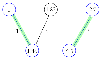
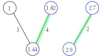
Although Figure 5 is a MCM, it is not a maximum weight matching. This leads to a smaller degree in our approximate GCD. However, Figure 6 is a maximum weight matching which gives us a higher degree GCD.
Finally we need to find , and .
Since the MWM given in Figure 6 contains two edges we have and
which will be presented by and . In order to get and , we write:
This gives us
Also we can write
VIII Concluding Remarks
This paper solves the approximate GCD problem in Lagrange bases. Our algorithm follows the ideas in [17] and [33]. The results of this work are relevant to approximate GCD for a specific pseudometric, namely the root pseudometric.
A possible extension of this work may be approximate GCD in Lagrange bases with respect to a different metric (or pseudometric). Moreover, the main algorithm of this paper can be trivially extended to Hermite basis. The only difference will be the rootfinding step. In order to compute the roots one can use the companion pencil presented in [13].
One may wonder why clustering is used in and separately in to identify common roots, instead of simply considering the roots of and together and then clustering them (and thus identifying common zeros and hence the GCD). We feel that a significant feature of approximate multiple zeros arising from a single polynomial is symmetry: computing results in a near-circular symmetric cluster near . There is no reason to believe that the perturbation in would even be the same magnitude, and in any case symmetry would be lost. We admit that this is a heuristic, and does not account for structured perturbations ; nonetheless we think this is a valuable heuristic and it has worked well for us in the examples that we have tried.
An interesting example, which we will describe in a future paper, is to cluster the roots of a Mandelbrot polynomial, defined as and . These are studied by homotopy methods in [14] using the homotopy which starts with double roots at : if one looks at the roots of and clusters into double roots, do we get approximations of roots of ? The answer is no, or not often, and then only in regions of sensitivity. But this example is, as mentioned in the previous paragraph, structured. We need to perform more experiments on this example before commenting further.
Finally, as it is described in this current paper, the clustering heuristic by distance, multiplicity, and symmetry does not take into any account that the points are actually supposed to be roots of a polynomial. Because it is based on the approximation
| (VIII.1) |
for an -fold zero, we should in practice post-process the clustering results, estimate the th derivative at a clustered root, and re-do the clustering with the “fuzz factors” of the heuristic replaced by the estimates resulting from the post-processing. This would increase our confidence that we had found an actual multiple root. Indeed one could imagine an iterative algorithm being based on this refinement step. We leave this to future work.
Acknowledgments
This work was supported by NSERC and the Ontario Research Centre for Computer Algebra. RMC thanks Laureano Gonzalez-Vega for a conversation in 1997 about the potential value of symmetry in clustering.
References
- [1] A. Amiraslani. Dividing polynomials when you only know their values. In Proceedings EACA, pages 5–10, 2004.
- [2] A. Amiraslani, R. M. Corless, L. Gonzalez-Vega, and A. Shakoori. Polynomial algebra by values. Technical report, Technical Report TR-04-01, Ontario Research Centre for Computer Algebra, 2004.
- [3] A. Amiraslani, R. M. Corless, and M. Gunasingam. Differentiation matrices for univariate polynomials. Numerical Algorithms, pages 1–31, 2018.
- [4] A. Amiraslani, R. M. Corless, and P. Lancaster. Linearization of matrix polynomials expressed in polynomial bases. IMA J. Numer. Anal., 29(1):141–157, 2009.
- [5] D. A. Aruliah, R. M. Corless, Laureano Gonzalez-Vega, and A. Shakoori. Geometric applications of the Bézout matrix in the Lagrange basis. In Proceedings of the 2007 international workshop on Symbolic-numeric computation, pages 55–64, 2007.
- [6] Ruben Becker, Michael Sagraloff, Vikram Sharma, Juan Xu, and Chee Yap. Complexity analysis of root clustering for a complex polynomial. In Proceedings of the ACM on International Symposium on Symbolic and Algebraic Computation, pages 71–78, 2016.
- [7] B. Beckermann. The condition number of real Vandermonde, Krylov and positive definite Hankel matrices. Numerische Mathematik, 85(4):553–577, 2000.
- [8] B. Beckermann and G. Labahn. When are two numerical polynomials relatively prime? Journal of Symbolic Computation, 26(6):677 – 689, 1998.
- [9] B. Beckermann, G. Labahn, and A. C. Matos. On rational functions without Froissart doublets. Numerische Mathematik, 138(3):615–633, 2018.
- [10] B. Botting, M. Giesbrecht, and J. May. Using Riemannian SVD for problems in approximate algebra. In Proceedings of the International Workshop of Symbolic-Numeric Computation, pages 209–219. Citeseer, 2005.
- [11] John C Butcher, Robert M Corless, Laureano Gonzalez-Vega, and Azar Shakoori. Polynomial algebra for Birkhoff interpolants. Numerical Algorithms, 56(3):319–347, 2011.
- [12] J. M. Carnicer, Y. Khiar, and J. M. Peña. Optimal stability of the Lagrange formula and conditioning of the Newton formula. Journal of Approximation Theory, 2017.
- [13] E. Y. S. Chan, R. M. Corless, and L. Rafiee Sevyeri. Generalized standard triples for algebraic linearizations of matrix polynomials, 2018.
- [14] Eunice Y. S. Chan. A comparison of solution methods for Mandelbrot-like polynomials. Master’s thesis, University of Western Ontario, 2016.
- [15] R. M. Corless. Generalized companion matrices in the Lagrange basis. In Proceedings EACA, pages 317–322. Santander, Spain: Universidad de Cantabria, 2004.
- [16] R. M. Corless, P. M. Gianni, B. M. Trager, and S. M. Watt. The singular value decomposition for polynomial systems. In Proceedings of the 1995 International Symposium on Symbolic and Algebraic Computation, ISSAC ’95, pages 195–207, New York, NY, USA, 1995. ACM.
- [17] R. M. Corless and L. Rafiee Sevyeri. Approximate GCD in a Bernstein basis. Springer, pages 77–91, 2020.
- [18] R. M. Corless and S. M. Watt. Bernstein bases are optimal, but, sometimes, Lagrange bases are better. In In Proceedings of SYNASC, Timisoara, pages 141–153. MIRTON Press, 2004.
- [19] Robert M Corless, Azar Shakoori, DA Aruliah, and Laureano Gonzalez-Vega. Barycentric Hermite interpolants for event location in initial-value problems. JNAIAM J. Numer. Anal. Indust. Appl. Math, 3:1–16, 2008.
- [20] Thomas H. Cormen, Charles E. Leiserson, Ronald L. Rivest, and Clifford Stein. Introduction to algorithms. MIT Press, Cambridge, MA; McGraw-Hill Book Co., Boston, MA, second edition, 2001.
- [21] Gema M Diaz-Toca, Mario Fioravanti, Laureano Gonzalez-Vega, and Azar Shakoori. Using implicit equations of parametric curves and surfaces without computing them: Polynomial algebra by values. Computer aided geometric design, 30(1):116–139, 2013.
- [22] Gema M. Diaz-Toca and Laureano Gonzalez-Vega. Computing greatest common divisors and squarefree decompositions through matrix methods: The parametric and approximate cases. Linear Algebra and its Applications, 412(2):222 – 246, 2006.
- [23] R. Duan and S. Pettie. Linear-time approximation for maximum weight matching. Journal of the ACM (JACM), 61(1):1–23, 2014.
- [24] R. T. Farouki and T. Goodman. On the optimal stability of the Bernstein basis. Mathematics of Computation of the American Mathematical Society, 65(216):1553–1566, 1996.
- [25] S. Fortune. Polynomial root finding using iterated eigenvalue computation. In Proceedings of the 2001 international symposium on Symbolic and algebraic computation, pages 121–128, 2001.
- [26] Rémi Imbach, Victor Y Pan, and Chee Yap. Implementation of a near-optimal complex root clustering algorithm. In International Congress on Mathematical Software, pages 235–244. Springer, 2018.
- [27] E. Kaltofen, Z. Yang, and L. Zhi. Structured low rank approximation of a Sylvester matrix. In Symbolic-numeric computation, pages 69–83. Springer, 2007.
- [28] N. K. Karmarkar and Y. N. Lakshman. Approximate polynomial Greatest Common Divisors and nearest singular polynomials. In Proceedings of the 1996 International Symposium on Symbolic and Algebraic Computation, ISSAC ’96, pages 35–39, New York, NY, USA, 1996. ACM.
- [29] N. K. Karmarkar and Y. N. Lakshman. On approximate gcds of univariate polynomials. Journal of Symbolic Computation, 26(6):653–666, 1998.
- [30] J. L. Kelley. General topology. Courier Dover Publications, 2017.
- [31] F. Le Gall. Powers of tensors and fast matrix multiplication. In Proceedings of the 39th international symposium on symbolic and algebraic computation, pages 296–303, 2014.
- [32] Y. Nakatsukasa, O. Sète, and L. Trefethen. The AAA algorithm for rational approximation. SIAM Journal on Scientific Computing, 40(3):A1494–A1522, 2018.
- [33] V. Y. Pan. Numerical computation of a polynomial GCD and extensions. Information and computation, 167:71–85, 2001.
- [34] L Rafiee Sevyeri. Hybrid Symbolic-Numeric Computing in Linear and Polynomial Algebra. PhD thesis, Western University, 2020.
- [35] N. Rezvani and R. M. Corless. Using weighted norms to find nearest polynomials satisfying linear constraints. In Proceedings of the 2011 International Workshop on Symbolic-Numeric Computation, SNC ’11, pages 81–87, New York, NY, USA, 2011. ACM.
- [36] Azar Shakoori. The Bézout matrix in the Lagrange basis. In Proceedings EACA, pages 295–299. Citeseer, 2004.
- [37] B. T. Smith. Error bounds for zeros of a polynomial based upon Gerschgorin’s theorems. Journal of the ACM (JACM), 17(4):661–674, 1970.
- [38] Z. Zeng. The approximate gcd of inexact polynomials. part I: a univariate algorithm. Proceedings of the 2004 international symposium on Symbolic and algebraic computation, ACM, pages 320–327, 2004.
- [39] Z. Zeng. The numerical greatest common divisor of univariate polynomials. Randomization, relaxation, and complexity in polynomial equation solving, 556:187–217, 2011.