Strong enhancement of heavy-hole Landé factor $q$ in InGaAs symmetric quantum dots revealed by coherent optical spectroscopy

In the field of quantum information, new applications based on spin qubits in solids are actively developed. Spin photonics studies based on coherent optical manipulation and measurement of spin qubits in semiconductor quantum dots (QDs) Imamoglu-review-NatPhot2015; Lodahl-NatNanoTech2018, color centers in diamond Diamond and SiC SiC as well as rare-earth-ion doped crystals rare_earth are heavily pursued. Here, the energy splitting of optical transitions into orthogonal linearly polarized spectral lines due to the Zeeman effect in a transverse magnetic field Zeeman-Nature1897 is used to address the electron spin qubit and achieve spin-photon entanglement using properly polarized and frequency shaped optical fields Imamoglu; Yamamoto; Steel. To manipulate electron spins in a deterministic way, a precise knowledge of the energy splitting and magnetic-field-induced optical anisotropy, i.e. the orientation of eigen polarizations for optical transitions with respect to the direction of magnetic field, is required.

In atomic gases the energy splitting is proportional to the magnetic field strength, $B$, and the Landé $g$ factor, spectral lines are polarized either along ($\pi$) or perpendicular ($\sigma$) to the magnetic field axis Zeeman-Nature1897. In solids, the crystal field and localization potential lead to a modification of the $g$ factor requiring a description of the $g$ factor by a tensor. Consequently, the resulting axes of optical anisotropy (eigen polarizations) do not necessarily coincide with the magnetic field direction, but depend on the mutual orientation of the vector ${\bm{B}}$ and the sample axes KusrayevPRL1999; Semenov-PRB2003; KoudinovPRB2004; Kiessling2006; Poltavtsev-PRR2020. In direct band gap III-V and II-VI bulk semiconductors with zinc-blende lattice (as well as in group IV semiconductors with diamond lattice), the top valence band is formed by the heavy- and light-hole branches degenerate at zero wave vector ${\bm{k}}=0$ ($\Gamma$ point) and the free-hole Zeeman splitting is dependent in a complicated way on the angle between the hole wave vector ${\bm{k}}$ and magnetic field.

In low-dimensional systems with sizes on a nanometer scale, size-quantization results in a splitting of the bulk heavy- and light-hole branches into two series of hole subbands, $hh\nu$ and $lh\nu$ with $\nu=1,2\dots$ In comparison with the T_d point-group symmetry of bulk zinc-blende semiconductors, (001)-grown quantum wells have a reduced symmetry D_2d. As shown in Ref. Marie1999, the in-plane $g$ factor of a $hh1$ heavy hole is very small and given by the value of $3q$, where $q$ is one of the two bulk Landé factor parameters introduced by Luttinger Luttinger. Most currently available self-assembled QDs have a reduced symmetry C_2v or lower than D_2d KoudinovPRB2004; Kiessling2006; Nenashev-PRB2003; Zinovieva2003; Skolnick-PRB2005; Babinski; Belhadj-APL2010; Yakovlev2011; DomeShape2005; Glasman; Zunger; Kazimierczu-PRB2016; Belykh2016. There are several reasons for the symmetry reduction, in particular, the asymmetry of a QD in the growth direction $z$ (e.g., pyramid-, lens- or dome-like shape of QDs), in-plane shape elongation, an in-plane strain etc., for more details see Ref. Zunger. These strongly inhomogeneous factors produce a strong scatter in the polarization eigenstates in the QD ensemble and present the major obstacle for optical manipulation of a spin-qubit ensemble which requires uniform magnetic-field-induced optical anisotropy in all QDs.

In this letter we study self-assembled (In,Ga)As/GaAs QDs grown under special conditions. These QDs show the higher symmetry tetragonal point group D_2d (or $\bar{4}2m$) that includes the mirror-rotation operation $S_{4}$ and, thereby, comprises symmetry along the growth axis. We have found that in these QDs, unlike in the (001)-grown quantum wells, the in-plane hole $g$ factor exceeds by far the bulk GaAs value $|3q|$. To explain this unexpected finding we propose a new mechanism contributing to the enhancement of heavy-hole Landé factor parameter $q$. The enhancment stems from the strong localization of the hole within a QD and is governed by the difference $\gamma_{3}-\gamma_{2}$ of Luttinger valence band parameters Luttinger which is responsible for the bulk valence band warping. The new mechanism is shown to dominate in symmetric QDs and leads to a uniform magnetic-field-induced optical anisotropy in the entire QDs ensemble. For the experimental confirmation, we have studied the coherent optical QD response in the form of spin dependent photon echoes from trions Poltavtsev-PRR2020 in singly electron charged QDs. The high symmetry of the QDs is confirmed by the dependence of photon echo signal on the orientation of external magnetic field with respect to the sample axes. The obtained in-plane hole $g$ factor value of about 0.2 associated with the proposed mechanism is comparable with that of the conduction band electron $g$ factor.

We study singly electron charged QDs and analyze the spin properties of a resident electron and a hole (in the trion) occupying the QD ground states $e1$ and $hh1$, respectively. First we perform a symmetry analysis of the Zeeman Hamiltonian for a nanostructure of the point-group D_2d. Then we analyze the consequences of possible symmetry-breaking distortions. In a structure of D_2d symmetry, the $e1$ conduction-electron and $hh1$ heavy-hole states transform according to the equivalent representations $\Gamma_{6}$ as the spinors $\psi^{e}_{1/2}=\uparrow\!S$, $\psi^{e}_{-1/2}=\downarrow\!S$ and pair of functions $\psi^{h}_{1/2}=\downarrow\!(X-{\rm i}Y)/\sqrt{2}$, $\psi^{h}_{-1/2}=-\uparrow\!(X+{\rm i}Y)/\sqrt{2}$, see Glasman; IvchPikusBook. Here $S$ and $X,Y$ are, respectively, the conduction-band and valence-band Bloch functions at the $\Gamma$ point. In the chosen bases, the Zeeman Hamiltonian matrices in the magnetic field ${\bm{B}}\perp z$ have the same structure

and differ only in the values of the in-plane $g$ factors, $g_{e}$ and $g_{h}$. Hereafter $\mu_{B}$ is the Bohr magneton, $x\parallel[100],y\parallel[010]$, and $\sigma_{x},\sigma_{y}$ are the Pauli 2$\times$2 matrices which coincide for electron and heavy hole. Note that, in the other frequently used hole basis $\tilde{\psi}^{h}_{1/2}=-\uparrow(X+{\rm i}Y)/\sqrt{2}$, $\tilde{\psi}^{h}_{-1/2}=\downarrow(X-{\rm i}Y)/\sqrt{2}$, the second term in ${\cal H}^{h}({\bm{B}})$ has the opposite sign.

The magnetic field splits the electron and hole spin states into the energy sublevels $E^{i}_{\pm}=\pm\mu_{B}|g_{i}|B/2$ ($i=e,h$). The selection rules for the optical transitions from the electron sublevel $E^{e}_{\pm}$ to the trion state with a pair of singlet electrons and a hole in the sublevel $E^{h}_{\pm}$ are shown in Fig. 1(a) for $g_{e}g_{h}>0$. The optical transitions are linearly polarized along the directions determined by the angles $\alpha_{1,2}$ between the polarization unit vector ${\bm{e}}$ and the $x$ axis. These angles are related to the angle $\varphi$ between the magnetic field vector and the $x$ axis (Fig. 1(b)) by

where D_2d indicates the QD symmetry. In spite of the isotropic Hamiltonians (1), the behaviour of $\alpha_{1}$ or $\alpha_{2}$ as a function of $\varphi$ reveals the tetragonal symmetry. Particularly, for $g_{e}g_{h}>0$ the transition $(e,+)\to(h,+)$ is polarized perpendicular to the magnetic field if ${\bm{B}}\parallel[100],[010],[\bar{1}00]$ or $[0\bar{1}0]$, while, for ${\bm{B}}\parallel[110],[\bar{1}10],[\bar{1}\bar{1}0]$ or $[1\bar{1}0]$, it is polarized along ${\bm{B}}$. The D_2d symmetry Hamiltonians (1) leads to a variation of the optical polarization described by the fourth harmonic as function of $\varphi$ Semenov-PRB2003.

If a nanostructure is distorted by a perturbation of the symmetry $B_{1}$ (like $x^{2}-y^{2}$) and/or $B_{2}$ (like $2xy$), where $B_{1}$ and $B_{2}$ are the irreducible representations of the D_2d group, then the Zeeman Hamiltonians have additional anisotropic contributions

where $g_{1i}$ and $g_{2i}$ relate to $B_{1}$ and $B_{2}$. The spin-split states have the energies $E^{e,h}_{\pm}=\pm\hbar\omega_{i}/2$ with the spin splitting given by $\hbar\omega_{i}=\tilde{g}_{i}\mu_{B}B$, where

$g_{i}^{\prime}=\sqrt{g_{1i}^{2}+g_{2i}^{2}}$ and $2\chi_{i}=\arctan{(g_{2i}/g_{1i})}$.

Because of the anisotropy caused by the distortion (3), the effective magnetic field $\tilde{\bm{B}}$ acting on the carrier is directed not along the vector ${\bm{B}}$ and has the angle

with the $x$ axis, the values of $\theta_{i}$ can cover the full circle (0, $2\pi$). The spin-split eigen states are given by

where $\varphi_{e}({\bm{r}})$ and $\varphi_{h}({\bm{r}})$ are the $e1$ and $hh1$ envelope functions, $\theta_{+}^{i}=\theta_{i}$ and $\theta_{-}^{i}=\theta_{i}+\pi$.

The optical transitions $e,\pm\to h,\pm$ and $e,\pm\to h,\mp$ are also linearly polarized as for a QD of D_2d symmetry. However, the corresponding eigen polarizations are now determined not by Eq. (2) but by the more general equations

For the experimental study of the Zeeman effect in transverse magnetic field we use an approach based on spin dependent photon echoes (PE) Poltavtsev-PRR2020. The advantage of this technique is the unique possibility of obtaining the full set of Zeeman splittings and optical anisotropy even if they are hidden by inhomogeneous broadening of the optical transitions. We study self-assembled (In,Ga)As/GaAs QDs grown by molecular beam epitaxy with subsequent annealing procedure as described in SM section I SupplMat. In order to increase light-matter coupling and PE signal amplitude Poltavtsev-PRB2016; Salewski-PRB2017; Kasprzak-Optica2018 four QD layers are placed in the antinodes of a standing electromagnetic wave of a weak-coupling microcavity with the quality factor $Q\sim 1000$ Kamenskii-PRB2020. Modulation doping with Si provides one resident electron to each QD on average.

The sample is placed into a superconducting split-coil cryostat and kept at the temperature of 1.4 K. The magnetic field is applied in Voigt geometry in the $xy$-plane and rotation of the sample around $z$-axis allows us to vary the angle $\varphi$. A sequence of two optical pulses with $2$ ps duration delayed by the $\tau_{12}$ time with respect to each other excites the QDs under nearly normal incidence (see details in SM section II SupplMat)). The photon energy is tuned into resonance with the cavity mode and set to 1.434 eV. The transient four-wave mixing signal is detected in reflection geometry using heterodyne detection PSS2018. Due to inhomogeneous broadening of the optical transitions in the ensemble of QDs the signal is represented by a photon echo which is delayed by $2\tau_{12}$ with respect to the first excitation pulse Poltavtsev-PRB2016. At $B=0$ the PE amplitude decays exponentially $\exp(-2\tau_{12}/T_2)$ with the optical coherence time $T_{2}=430$ ps as shown in Fig. 4(a). For $B\neq 0$ the PE signal shows oscillations due to spin precession of electrons and holes. Such spin dependent PE signal is sensitive to the polarization configuration of the excitation pulses LangerPRL. Using linearly polarized optical pulses allows us to determine precisely the eigen polarizations $\alpha_{1,2}$ as a function of $\varphi$ Poltavtsev-PRR2020. In what follows we concentrate on the HVH polarization configuration where the first pulse is polarized along the horizontally (H) oriented field ${\bm{B}}$, while the polarization of the second pulse is vertical (V). The detection of PE is performed in H polarization.

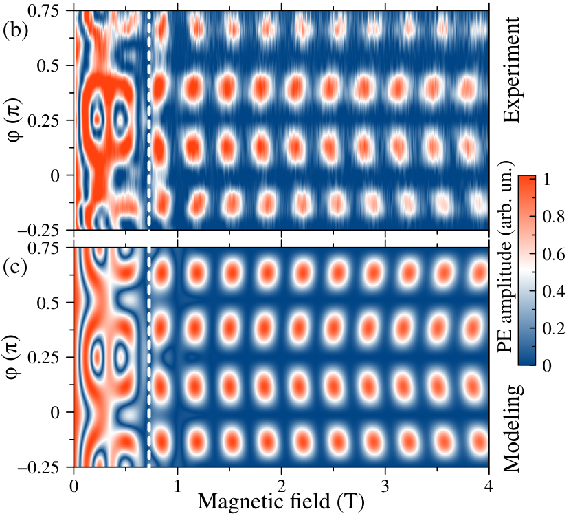
Figure 4(b) shows experimental data for the spin dependent PE amplitude as a function of $\varphi$ and $B$ at a fixed value $\tau_{12}=400$ ps (vertical dashed line in Fig. 4(a)) measured in a steps of $\pi/18$. Two types of oscillations are observed. First, there are oscillations along the $B$-axis due to variation of Larmor precession frequencies of electrons $\omega_{e}$ and holes $\omega_{h}$. Second, angular $\varphi$ oscillations appear because of the dependence of $\alpha_{1,2}$ on $\varphi$. The signal behaves differently for the ranges $B\leq 0.7$ T and $B\geq 0.7$ T separated by the vertical dashed line in Fig. 4(b). This is attributed to the large spread of hole $g$ factor, $\Delta g_{h}$, which results in decay of the hole spin precession contribution to the PE signal. Nevertheless, optical anisotropy can be evaluated from the angular dependence even for large $B$, where the PE amplitude $P_{HVH}$ is decribed by the simple relation (see SM section III SupplMat)

In this case, the magnetic field and the delay $\tau_{12}$ oscillations of the PE signal are associated only with the electron spin precession. It follows from Eq. (20), that the D_2d symmetry contribution ($\alpha_{1}=-\varphi$) gives rise to the eighth harmonic in the $P_{HVH}(\varphi)$ dependence. By contrast, for the C_2v symmetry the hole contribution $\alpha_{1}=-\chi_{h}/2$ (see Eqs. (4),(7)) the angular dependence contains the fourth harmonics.

The angular dependence in Fig. 4(b) at $B>0.7$ T shows four oscillations within the range $0\leq\varphi\leq\pi$, i.e. we observe the eighth harmonics. The contrast of oscillations $C=(P_{\rm max}-P_{\rm min})/(P_{\rm max}+P_{\rm min})\approx 0.95$ is very high, where $P_{\rm max}$ and $P_{\rm min}$ are the maximum and minimum values of $|P_{HVH}|$. Thus we conclude that the D_2d symmetry gives the main contribution to the hole $g$ factor. Moreover, the high contrast of angular oscillations indicates that the spread of directions of eigen-polarizations (spread of $\alpha_{1}$) in the QDs ensemble under study is small SupplMat.

In order to determine accurately the dependences $\tilde{g}_{i}=\hbar\omega_{i}/\mu_{B}B$ on $\varphi$ we analyze the PE transients for different values of $B$, polarization configurations and sample orientations. The details of fitting are presented in SM section IV SupplMat. The analysis shows no dependence of $\tilde{g}_{e,h}$ on magnetic field strength. The obtained angular dependences of electron and hole $g$ factors are shown in Fig. 3 by red dots. As one can see, the value of $\tilde{g}_{e}$ changes between $0.52$ and $0.54$ and can be fitted by Eq. (4) (solid line) with parameters $g_{e}=-0.531$, $g^{\prime}_{e}=0.007$, $\chi_{e}=0$, where we take into account that in (In,Ga)As QDs ${g}_{e}<0$ Belykh2016; Nakaoka-PRB2005; YugovaPRB2005. Thus, the direction of the effective magnetic field ${\tilde{\bm{B}}}$ negligibly deviates from ${\bm{B}}$ by less than $1^{\circ}$.

The angular dependence of $\tilde{g}_{h}$ clearly indicates that both D_2d and low-symmetry contributions have impact on the hole’s $g$ factor Semenov-PRB2003; Poltavtsev-PRR2020. Here, a weak low-symmetry contribution is added to the dominant D_2d contribution. The dependence of $\tilde{g}_{h}(\varphi)$ can be approximated by Eq. (4) with $g_{h}=0.213$, $g^{\prime}_{h}=0.029$, and $\chi_{h}=\pi/2$, as shown in Fig. 3(b). The positive sign of $g_{h}$ follows from the theoretical model which is presented below. The calculated dependencies of PE amplitude on $B$ and $\varphi$ with the obtained electron and hole $g$ factor tensors are shown in Fig. 4(c). The excellent correspondence between experimental and theoretical figures in Figs. 4(b) and 4(c) confirms the accuracy of the analysis above.

The obtained values of $g_{h}$ and $g^{\prime}_{h}$ are non-trivial. In a zinc-blende quantum well (QW) structure grown along the [001] direction $g_{h}=3q$, where $q$ is the negative Landé valence-band parameter of the bulk semiconductor (in Ref. Marie1999 a value of $-3q$ is used with positive $q$). One of the aims of our work is to demonstrate that in a quantum dot having D_2d symmetry the quantum confinement in the $xy$-plane can result in a remarkable enhancement of the factor $|3q|$. This can be understood taking into account the expansion of the heavy-hole Zeeman Hamiltonian in powers of wave vector ${\bm{k}}$ Marie1999

resulting in the renormalization of the hole $g$ factor given by $g_{h}({\bm{k}})=3q+ck^{2}+\dots$ The coefficient $c$ can be conveniently presented as $G(\gamma_{3}-\gamma_{2})L_{W}^{2}$, where $\gamma_{2}$ and $\gamma_{3}$ are the dimensionless Luttinger valence-band parameters and $L_{W}$ is the QW width, for a GaAs-based QW the coefficient $G$ takes the value of 0.08 (see details in SM section V SupplMat). The factor ${\gamma_{3}-\gamma_{2}}$ shows that $c$ is related to the bulk valence band warping. At low temperature the value of $ck^{2}$ in a QW is small compared to $3q$ and can be ignored Marie1999. In a QD, $k^{2}$ should be averaged over the quantum-confined state leading to

where $3q_{w}=c\left<k^{2}\right>$, and therefore the parameter $q$ is renormalized by a factor of $1+(q_{w}/q)$. For a quantum dot-disk of radius $R$ we obtain $3q_{w}\approx 0.4\ (L_{W}/R)^{2}$. For a parabolic GaAs-based QD with the confining potential $V({\bm{r}})=[\kappa_{z}z^{2}+\kappa_{\parallel}(x^{2}+y^{2})]/2$, we have $3q_{w}\approx 0.5\sqrt{\kappa_{\parallel}/\kappa_{z}}$. For the aspect ratios $2R$:$L_{W}$=3:1 and $\kappa_{z}$:$\kappa_{\parallel}$= 3:1, the quantum-confinement contribution $3q_{w}\approx 0.3$ by far exceeds the experimentally measured bulk value $|3q|\approx 0.035$ Marie1999. Note that, with decreasing $R$ values or increasing $\kappa_{\parallel}$ values the higher orders terms in the expansion (9) should be also taken into account and the above estimates of $q_{w}$ give only its order of magnitude.

In the existing theories of the heavy-hole in-plane Landé factor in QWs and QDs of the symmetry C_2v or lower, the values $g_{1h}$ or $g_{2h}$ are determined by the heavy-light hole mixing induced by the distortions Semenov-PRB2003; Nenashev-PRB2003; Zinovieva2003; KoudinovPRB2004; Kazimierczu-PRB2016; PikusPikus. In the proposed enhancement of the parameter $q$ in QDs of D_2d symmetry, the Bloch heavy- and light-hole functions are naturally mixed by the hole nonzero wave vectors ${\bm{k}}$ and the quantization of $k^{2}$ in QDs causes the renormalization of $q$.

The theory gives two important predictions. First, because of opposite signs of $q$ and $c$, there are QDs with larger base size where $3q$ and $3q_{w}$ compensate each other and the in-plane $g$ factor vanishes. Second, besides the term $ck^{2}$ in Eq. (9), there is an additional term $\delta{\cal H}({\bm{B}},{\bm{k}})=(\mu_{B}/2)c^{\prime}(\sigma_{+}B_{+}k_{-}^{2}+\sigma_{-}B_{-}k^{2}_{+})$ Marie1999; Miserev, where $\sigma_{\pm}=(\sigma_{x}\pm{\rm i}\sigma_{y})/2$ and $c^{\prime}=[(\gamma_{3}+\gamma_{2})/(\gamma_{3}-\gamma_{2})]c$. In a QD of D_2d symmetry this term does not contribute to the hole $g$ factor. However, for a QD shape of reduced symmetry the average values of $\langle k^{2}_{x}-k^{2}_{y}\rangle$ and $\langle 2k_{x}k_{y}\rangle$ do not vanish and the corresponding terms have an impact to low symmetry contribution through the coefficients $g_{1h}$ and $g_{2h}$ in Eq. (3).

In conclusion, we have revealed experimentally and theoretically that the surprisingly large in-plane hole $g$ factor in an ensemble of strongly annealed (In,Ga)As/GaAs QDs is dominated by the D_2d symmetry contribution. The proposed enhancement of the Landé valence-band parameter $q$ in QDs of the D_2d symmetry allows us to explain the unique angular patterns of spin dependent photon echoes in the in-plane magnetic field. The enhancement appears because of the in-plane confinement of holes and the valence band warping. It results in the uniform magnetic-field-induced optical anisotropy for the entire quantum dot ensemble which is highly appealing for application in quantum information devices.