Evidential fully convolutional network for semantic segmentationJournal: Applied Intelligence

The main concepts underlying DS theory are only briefly presented in this section, and some basic notations are introduced. Detailed information can be found in Shafer’s original work shafer1976mathematical and in the recent review denoeux20b.

Let $\Omega=\{\omega_{1},\ldots,\omega_{M}\}$ be a set of classes, called the frame of discernment. A mass function on $\Omega$ is a mapping $m$ from $2^{\Omega}$ to [0,1] such that $m(\emptyset)=0$ and

For any $A\subseteq\Omega$, each mass $m(A)$ is interpreted as a share of a unit mass of belief allocated to the hypothesis that the truth is in $A$, and which cannot be allocated to any strict subset of $A$ based on the available evidence. Set $A$ is called a focal set of $m$ if $m(A)>0$. A mass function is said to be logical if it has only one focal set.

Two mass functions $m_{1}$ and $m_{2}$ representing independent items of evidence can be combined conjunctively by Dempster’s rule $\oplus$ shafer1976mathematical as

and $(m_{1}\oplus m_{2})(\emptyset)=0$. Mass functions $m_{1}$ and $m_{2}$ can be combined if and only if the denominator on the right-hand side of Eq. (2a) is strictly positive. The operator $\oplus$ is commutative and associative.

For decision-making with belief functions, let $u_{ij}\in[0,1]$ denote the utility of selecting $\omega_{i}$ when the true state is $\omega_{j}$, and $f_{\omega_{i}}$ the act of selecting $\omega_{i}$. We define the pignistic expected utility denoeux2019decision of act $f_{\omega_{i}}$ as

Denœux denoeux2000neural proposed a distance-based neural-network based on DS theory, known as the evidential neural network (ENN) classifier. The ENN classifier summarizes the learning set by a small number of prototypes, and treats the proximity of an input vector to each prototype as a piece of evidence about its class. The different pieces of evidence are represented by mass functions, which are combined using Dempster’s rule (2). This section provides a brief description of the ENN classifier.

We consider a training set ${{\cal X}=\left\{\boldsymbol{x}^{1},\ldots,\boldsymbol{x}^{N}\right\}\subset\mathbb{R}^{P}}$ of $N$ examples represented by $P$-dimensional feature vectors, and $n$ prototypes $\{\boldsymbol{p}^{1},\ldots,\boldsymbol{p}^{n}\}\subset\mathbb{R}^{P}$. For a test sample $\boldsymbol{x}$, the ENN classifier constructs mass functions that quantify the uncertainty about its class in $\Omega=\{\omega_{1},\ldots,\omega_{M}\}$, using a three-step procedure. This procedure can be implemented in a neural-network layer, which will be plugged into an FCN model as explained in Section 3.1. The three-step procedure can be described as follows.

Step 1:

The similarity between $\boldsymbol{x}$ and each prototype $\boldsymbol{p}^{l}$ is computed as

$$s^{l}=\alpha^{l}\exp\left(-\left(\eta^{l}d^{l}\right)^{2}\right),\quad l=1,\ldots,n,$$

(4)

where $d^{l}={\left\|\boldsymbol{x}-\boldsymbol{p}^{l}\right\|}$ is the Euclidean distance between ${\boldsymbol{x}}$ and prototype ${\boldsymbol{p}}^{l}$, $\eta^{l}\in\mathbb{R}$ is a scale parameter and $\alpha^{l}$ is a parameter in $[0,1]$. Prototypes $\boldsymbol{p}^{1},\ldots,\boldsymbol{p}^{n}$ can be considered as vectors of connection weights between the input layer and a hidden layer of $n$ Radial Basis Function (RBF) units. The number $n$ of prototypes is a hyper-parameter and can be tuned using a validation set or by cross-validation.

Step 2:

The mass function $m^{l}$ associated to reference pattern $\boldsymbol{p}^{l}$ is computed as

	$\displaystyle m^{l}(\{\omega_{j}\})$	$\displaystyle=v_{j}^{l}s^{l},\quad j=1,\ldots,M$		(5a)
	$\displaystyle m^{l}(\Omega)$	$\displaystyle=1-s^{l},$		(5b)

where $v_{j}^{l}\geq 0$ is the degree of membership of prototype ${\boldsymbol{p}}^{l}$ to class $\omega_{j}$ with $\sum_{j=1}^{M}v_{j}^{l}=1$. We denote the vector of masses induced by prototype ${\boldsymbol{p}}^{l}$ as

$$\boldsymbol{m}^{l}=(m^{l}(\{\omega_{1}\}),\ldots,m^{l}(\{{\omega}_{M}\}),m^{\mathit{l}}(\Omega))^{T}.$$

Eq. (5) can be regarded as computing the activation of units in a “mass functions” layer composed of $n$ modules of $M+1$ units each. The activations of the units in module $l$ correspond to the belief masses assigned by $m^{l}$.

Step 3:

The $n$ mass functions $\boldsymbol{m}^{l}$, $l=1,\ldots,n$, are aggregated by Dempster’s rule (2). The combined mass function can be computed iteratively as $\mu^{1}=m^{1}$ and $\mu^{l}=\mu^{l-1}\cap m^{l}$ for $l=2,\ldots,n$. From (2a), we have

	$$\mu^{l}(\{\omega_{j}\})=\mu^{l-1}(\{\omega_{j}\})m^{l}(\{\omega_{j}\})+\\ \mu^{l-1}(\{\omega_{j}\})m^{l}(\{\Omega\})+\mu^{l-1}(\Omega)m^{l}(\{\omega_{j}\})$$		(6a)
for $l=2,\ldots,n$ and $j=1,\ldots,M$, and
	$$\mu^{l}(\Omega)=\mu^{l-1}(\Omega)m^{l}(\Omega)\quad l=2,\ldots,n.$$		(6b)

The output vector $\boldsymbol{m}=(m(\{\omega_{1}\}),\ldots,m(\{{\omega}_{M}\}),m(\Omega))^{T}$ is finally obtained by normalizing $\mu^{n}$ as

$$m(A)=\frac{\mu^{n}(A)}{\mu^{n}(\Omega)+\sum_{j^{\prime}=1}^{M}\mu^{n}(\{\omega_{j^{\prime}}\})},$$

with $A\in\{\{\omega_{1}\},\ldots,\{\omega_{M}\},\Omega\}$.

The network parameters are the prototypes $\boldsymbol{p}^{l}$, the coefficients $\alpha^{l}$ and $\eta_{l}$, and the membership degrees $v^{l}_{j}$ for $l=1,\ldots,n$ and $j=1,\ldots,M$. They are learnt by minimizing a loss function. To enforce the constraints $0\leq\alpha^{l}\leq 1$, we introduce new variables $\xi^{l}\in\mathbb{R}$ such that

Similarly, the constraints on parameters $v^{l}_{j}$ are enforced by introducing new parameters $\delta_{j}^{l}\in\mathbb{R}$ such that

for $l=1,\ldots,n$ and $j=1,\ldots,M$. More details can be found in denoeux2000neural.

The performance of an ENN classifier in semantic segmentation tasks heavily depends on the information contained in its input features. Feature representation, an essential part of the machine learning workflow, consists in discovering the predictors needed for semantic segmentation from input images. In recent years, FCNs long2015fully and their variants noh2015learning; krahenbuhl2011efficient have achieved remarkable performances thanks to their ability to construct rich pixel-wise deep feature representations.

FCNs owe their name to their architecture, which is built only from locally connected layers, such as convolution, pooling, and upsampling layers. No dense layer is used in this kind of architecture. Generally, an FCN consists of two main parts: an encoder-decoder architecture for pixel-wise object representation and a softmax layer for pixel-wise assignments. In the encoder-decoder architecture, an input image is encoded by several convolutional and pooling layers and then decoded by one or more upsampling layers. The softmax layer assigns each pixel in the input image to one of the classes based on the outputs of the encoder-decoder architecture. Therefore, the outputs of the encoder-decoder architecture, called the pixel-wise feature maps, are considered as a feature representation of the input image. In the study, these feature maps are used as input to a DS layer allowing for set-valued semantic segmentation, as will be shown in Section 3.1.

To understand the feature representation of FCNs, we briefly recall the encoder-decoder architecture illustrated in Figure 1. The encoder part consists of several convolutional and pooling layers. Each convolutional layer performs convolutions its input to produce a set of feature maps. Let $\boldsymbol{z}=(z^{1},\dots,z^{D})$ be the input made up of $D$ input maps or input channels $z^{i}$ ($i=1,\dots,D$) of size $H\times W$. The processes in a convolutional layer with input $\boldsymbol{z}$, consisting of $e$ convolution kernels with size $a\times b$, are expressed as

where $\varepsilon^{i,j}$, a matrix of size $a\times b$, is the convolution kernel between the $i$-th input map and the $j$-th output map; $\lambda^{j}$ is the bias of kernel $\varepsilon^{i,j}$; $\ast$ denotes the convolution operation; $c^{j}$ is the $j$-th output feature map, with size $\frac{h-a+1}{r}\times\frac{w-b+1}{r}$, $j=1,\dots,e$; $r$ is the stride with which the kernel slides over input map $z^{i}$, and $f$ is the activation function, such as the rectified linear unit $\textsf{ReLU}(x)=\max(0,x)$ 5459250. A pooling layer follows the convolutional layer to sub-sample feature map $c^{j}$ by computing some statistics of feature values within non-overlapping $s\times s$ windows. In the case of max-pooling used in this paper, the statistic is the maximum. Thus, the outputs of the pooling layer is composed of the $D$ feature maps sub-sampled by factor $s$. For example, feature map $c^{j}$ with size $\frac{h-a+1}{r}\times\frac{w-b+1}{r}$ is downsized to $\frac{h-a+1}{2r}\times\frac{w-b+1}{2r}$ by a pooling layer with a $2\times 2$ non-overlapping window.

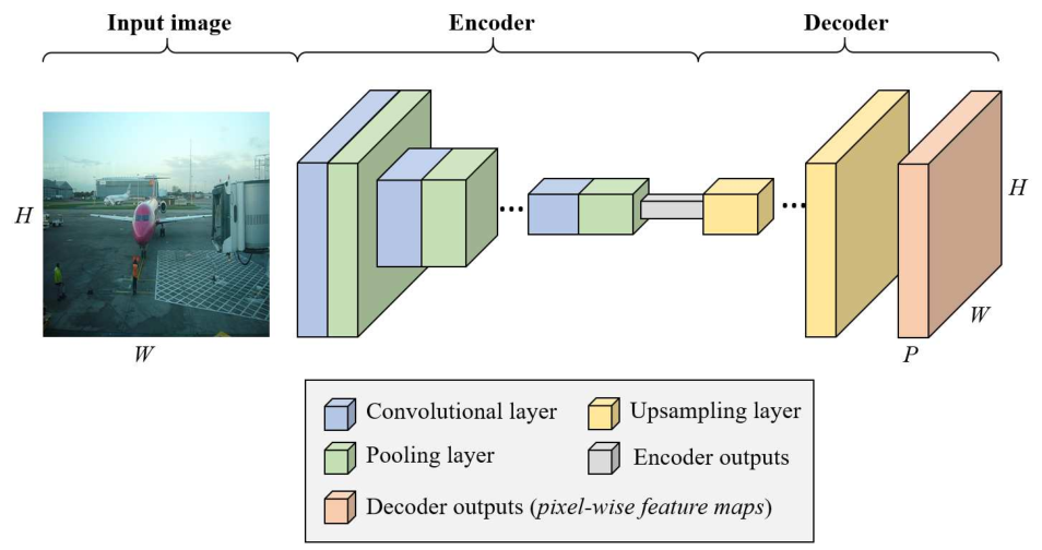
Although the convolution and pooling operations in the encoder part help feature representation by retaining only robust activations, spatial information within a receptive field is lost, which may be critical for image semantic segmentation. To address the issue, a decoder part made up of one or more upsampling layers is added at the output of the encoder part. The decoder performs the reverse operation of convolution and pooling for reconstructing a set of activations with the same size of the input image, as shown in Figure 1. Thus, the outputs of the decoder part are enlarged feature maps. In the study, we use a deconvolution layer noh2015learning to implement the upsampling operation.

A deconvolutional layer densifies its inputs of sparse feature maps through convolution-like operations with multiple learned kernels. However, contrary to convolutional layers, which connect multiple inputs within a kernel to a single activation, a deconvolutional layer associates a single input in a feature map to multiple outputs. Thus, the outputs of a deconvolutional layer are enlarged and dense feature maps. The processes of a deconvolution operation can also be summarized as Eq. (8), but its kernel sizes are larger than the input sizes, i.e., $a\geq H$ and $b\geq W$.

The main idea of this work is to hybridize the ENN classifier presented in Section 2.2 and the FCN recalled in Section 2.3 by “plugging” a DS layer followed by a utility layer at the output of the final deconvolutional layer in the FCN. The architecture of the proposed method, called the evidential FCN (E-FCN), is illustrated in Figure 2. An E-FCN classifier performs set-valued semantic segmentation and quantifies the uncertainty about the class of each pixel, taking values in $\Omega=\{\omega_{1},\ldots,\omega_{M}\}$, using a three-step procedure defined as follows.

•

Step 1: As in a probabilistic FCN (P-FCN), an image of size $W\times H\times 3$ is presented as input to the the encoder-decoder architecture of an FCN to generate pixel-wise feature maps of size $W\times H\times P$, where $P$ is the number of output channels. Each feature vector $1\times 1\times P$ from a pixel-wise feature map is a $P$-dimensional representation of the corresponding pixel, ready to be fed into the DS layer. This architecture generates reliable pixel-wise representations of the input image. Thanks to the representations, the E-FCN yields similar or even better performance for precise semantic segmentation than does a P-FCN with the same encoder-decoder architecture, as will be shown in Section 4.2.

•

Step 2: Each feature vector from the encoder-decoder architecture is fed into the DS layer, in which it is converted into a mass function as explained in Section 2.2. The output of the DS layer for a given feature vector is an $(M+1)$-dimensional mass vector

$$\boldsymbol{m}=(m(\{\omega_{1}\}),\ldots,m(\{{\omega}_{M}\}),m(\Omega))^{T}.$$

Thus, given pixel-wise feature maps of size $W\times H\times P$ from Step 1, the output of the DS layer is a tensor of size $W\times H\times(M+1)$. Each mass vector in the tensor represents the uncertainty about the class of the corresponding pixel. More precisely, the mass $m(\{\omega_{i}\})$ is a degree of belief that the ground truth of the pixel is $\omega_{i}$. The DS layer tends to allocate uniform masses if the representations contain confusing information. The additional degree of freedom $m(\Omega)$ makes it possible to quantify the lack of evidence denoeux2019logistic and verify whether the model is well trained tong2019ConvNet. The advantages of this uncertainty representation will be demonstrated in the performance evaluation of set-valued semantic segmentation using E-FCN in Section 4.3.

•

Step 3: The output pixel-wise mass vectors are fed into a utility layer for semantic segmentation, which is used to compute the expected utility of acts. Each act is defined as the assignment of a pixel to a non-empty subset $A$ of $\Omega$. Therefore, the output of the layer for each feature vector from Step 2 is an expected-utility vector at most equal to $2^{\Omega}-1$ when all of the possible acts are considered. The utility layer allows the E-FCN to perform set-valued semantic segmentation. This capability will be demonstrated by the performance comparison between the two types of FCNs in the tasks of set-valued segmentation (Section 4.3) and novelty detection (Section 4.4). More details of the utility layer for set-valued segmentation are introduced in the next section.

In this section, we describe in greater detail the decision-making process taking place in the utility layer. Section 3.2 begins with introducing the precise semantic segmentation method using mass functions and utilities. Section 3.2 describes a method for computing the utility of set-valued pixel-wise classification, after which an approach to set-valued classification based on mass functions is described in Section 3.2. In Section 3.2, we summarize the work ow as a neural network layer for the E-FCN model.

In traditional learning systems for image semantic segmentation, all pixels are labeled with a single class even when their true class cannot be determined with full certainty. For example, the true class may be uncertain at object borders, but the border pixels are still given precise labels. Additionally, one cannot reliably label some small objects in an image, such as distant objects in a driving scene. Arbitrarily giving precise labels to pixels with confusing information may have negative effects on learning systems for image semantic segmentation. The notion of soft label come09; denoeux19f may be a way to solve this problem.

Here, we define a soft label as a nonempty subset $A_{\ast}\in 2^{\Omega}\backslash\emptyset$ of classes a pixel may belong to, based on our current knowledge. For example, label $A_{\ast}=\{\omega_{i},\omega_{j}\}$ indicates that the true class of a pixel is known to be either $\omega_{i}$ or $\omega_{j}$ but we cannot determine which one specifically. A strategy of end-to-end learning is proposed to train an E-FNC from an image learning set with soft labels. All parameters in the DS layer are first initialized randomly using normal distributions. For a given pixel with nonempty soft label $A_{\ast}\subseteq\Omega$, let $m_{l}$ be the logical mass function with focal set $A_{\ast}$, i.e., such that $m_{l}(A_{\ast})=1$. The labeling pignistic expected utilities $\mathbb{E}_{\boldsymbol{m}_{l}}(f_{A})$ for $A\in 2^{\Omega}\backslash{\emptyset}$ can be computed using Eq. (14) and the pignistic belief-probability transformation Eq. (3b). Similarly, we consider the predicted pignistic expected utilities $\mathbb{E}_{m}(f_{A})$ for $A\in 2^{\Omega}\backslash\emptyset$ , where $m$ is the predicted mass function from the DS layer of the E-FCN, with focal sets $\{\omega_{1}\},\ldots,\{\omega_{M}\},\Omega$. For a given pixel with soft label $m_{l}$ and predicted mass function $m$, the loss $\mathcal{L}(m,m_{l})$ is defined as the squared Euclidean distance between the vectors of expected utilities w.r.t. $m_{l}$ and $m$:

The derivatives of $\mathcal{L}_{p}(m,m_{l})$ of the error w.r.t the output masses $m(\{\omega_{k}\})$ are

where $\delta_{kj}=1$ if $k=j$ and $\delta_{kj}=0$ otherwise. The derivatives of $m(\{\omega_{k}\})$ w.r.t $p^{l}_{k}$, $\eta^{l}$, and $\xi^{l}$ in the DS layer are the same as in Denœux’s original work denoeux2000neural, and the gradient with respect to all network parameters can be back-propagated from the output layer to the input layer.

In precise segmentation, each pixel of an image is assigned to exactly one class, the set of acts being defined as $\mathcal{F}=\{f_{\omega_{1}},\dots,f_{\omega_{M}}\}$. Three databases without soft labels mentioned in Section 4.1 were used to train and test the E-FCNs and probabilistic FCNs (P-FCNs). The metrics defined in Section 4.1 with the utility matrix ${\boldsymbol{U}}$ equal to the identity matrix were used for performance assessment.

In the experiment with each database, three widely used encoder-decoder architectures were combined with the DS and utility layers, as shown in Table 4. All encoder-decoder architectures in Table 4 have the same encoder part, which consists of four stages and two convolutional layers with $3\times 3$ kernels. Each stage is made up of three convolutional layers with $3\times 3$ kernels and a max-pooling layer with a $2\times 2$ non-overlapping window. Figure 4a illustrates the differences between the FCN-32s, FCN-16s, and FCN-8s architectures in their decoder parts with a deconvolutional layer. The FCN-SegNet architecture uses four deconvolutional layers to upsample the sparse feature maps from the end of the encoder part, as well as the feature maps from the corresponding pooling layers based on pooling indices badrinarayanan2017segnet, as shown in Figure 4b. The FCN-DilatedVGG architecture is the same as FCN-SegNet except that it adds a fully connected conditional random field at the end of the last deconvolutional layer chen2017deeplab. The numbers $P$ of feature maps for the Pascal, MIT and SIFT databases were, respectively, 31, 128 and 64. The numbers $n$ of prototypes in the DS layer for these three databases were set, respectively, to 75, 300 and 95.

The DS and utility layers slightly improve the accuracy of precise assignments performed by FCN models, even though the performance of FCN models on precise segmentation mainly depends on the encoder-decoder architecture. Table 4a presents the results of PU and UIoU for the Pascal VOC database. E-FCNs achieved higher PU and UIoU than P-FCNs with the same encoder-decoder architecture, which shows the E-FCNs outperform the P-FCNs for precise segmentation. Similar improvements can also be found in the MIT-scene Parsing and SIFT Flow databases as shown, respectively, in Tables 4b and 4c.

The use of DS and utility layers also makes the FCN models better calibrated. Figure 5 presents a visual calibration representation of the FCN-8s models in the Pascal VOC database. The top row shows the pixel distribution of prediction confidence (22b) as histograms. The average confidence of the E-FCN-8s model closely matches its average pixel utility, while the average confidence of the P-FCN-8s model is substantially higher than its average pixel utility. This is further illustrated in the bottom row of pixel utility diagrams, which show pixel utility as a function of confidence. The E-FCN-8s model is well calibrated since its confidence in each bin approximates the expected average utility, whereas the predicted utility of the P-FCN-8s model does not match its confidence. As a consequence, the E-FCN-8s model achieves a smaller ECE than the probabilistic one. The effect of the DS and utility layers on the calibration can also be found in the FCN-SegNet and FCN-DialtedVGG models on the MIT-scene Parsing and SIFT Flow databases as shown, respectively, in Figures 6 and 7.

In imprecise segmentation, each pixel of an image is assigned to a non-empty subset $A$ of $\Omega$; the set of acts is $\mathcal{F}=\{f_{A},A\in 2^{\Omega}\backslash{\emptyset}\}$, or a subset thereof. Here we only considered acts $f_{A}$ such that $A$ is a singleton, $\Omega$ or one of the soft labels in the training set. For performance evaluation, we used the metrics and the three databases described in Section 4.1. For each database, the segmentation masks with and without soft labels were used to train different FCN models. The same encoder-decoder architectures used for precise segmentation in Section 4.2 were combined with the DS and utility layers.

Figure 8 displays the test results according to PU and UIoU for imprecise segmentation of the Pascal VOC database. For a wide range of imprecision tolerance degree $\gamma$, the E-FCN models reach higher PU and UIoU values than those obtained by the P-FCN models; this is due to the fact that the E-FCN models tend to assign ambiguous pixels to multi-class sets, instead of making precise decisions. Such imprecise assignments avoid pixel-wise misclassification in case of high uncertainty, especially when feature vectors from an encoder-decoder architecture do not contain sufficient information to identify a precise class, and multiple classes have similar probabilities. Figure 9 shows the pixel confidence distributions for the FCN models with $\gamma=0.8$. We can see that the average confidences of the E-FCN models are smaller than those of the P-FCN models. This observation suggests that the E-FCN models make cautious decisions for ambiguous pixels by assigning them to multi-class sets, rather than classifying them arbitrarily into a single class. The E-FCN models are thus better calibrated than those based on P-FCN, which can be over-confident. Similar results are observed with the MIT-scene Parsing (Figures 10-11) and SIFT Flow (Figures 12-13) databases. We can thus conclude the DS and utility layers improve the performance of the FCN models in imprecise segmentation tasks by allowing us to assign some ambiguous pixels to multi-class sets.

In Figures 8, 10 and 12, we can see that the value of UIoU first increases and then decreases when $\gamma$ increases from 0.5 to 1. To explain this behavior, Figure 14 illustrates some segmentation examples generated by the E-FCN-8s model trained on the Pascal VOC database with soft labels. The first and second columns of Figure 14 contain, respectively, the original images and their precise segmentation predicted masks, while the third to sixth columns show the imprecise segmentation results for values of $\gamma$ ranging from 0.6 to 0.9. When $\gamma$ increases from 0.5 to 0.8, the majority of the green masks (the areas whose pixels are assigned to multi-class sets) tends to cover the red masks (the areas whose pixels are incorrectly classified in the precise segmentation). This observation can be explained by the fact that, in Eq. (20), the increase in the utility of the intersection between predicted and labeled areas is larger than the increase in the union between the two areas. As a result, UIoU increases when $\gamma$ increases from 0.5 to 0.8. However, when $\gamma$ increases from 0.8 to 1.0, the majority of the green masks cover the areas predicted correctly in the precise segmentation, which causes the increase in the utility of intersection to be smaller than the increase in the union areas. This phenomenon leads to the decrease of UIoU when $\gamma$ is larger than 0.8.

The use of soft labels improves the performance of the FCN models for imprecision segmentation tasks. As shown in Figure 8, the FCN models trained by the Pascal VOC database with soft labels have larger testing PU and UIoU than the ones without soft labels, which demonstrates the accuracy improvement using soft labels. Additionally, the use of soft labels can also improve the calibration of the FCN models. Figure 15 shows that the ECEs and bin gaps in the E-FCN and P-FCN models are smaller when using the learning set with soft labels. These results demonstrates the feasibility of processing pixels with confusing information by using soft labels when training FCN models. The improvement of accuracy and calibration due to learning from soft labels can also be found with the MIT-scene Parsing and SIFT Flow databases, as shown, respectively, in Figures 16 and 17. Therefore, we can conclude that the use of soft labels improves the accuracy and calibration of FCN models.

For novelty detection, a pixel is considered as an outlier or an ambiguous sample if it is assigned to set $\Omega$. Figures 18, 19 and 20 show the results of novelty detection using the E-FCN and P-FCN models when the learning set is extracted, respectively, from the Pascal VOC, MIT-scene Parsing and SIFT Flow databases, and the test set is composed of images from the other two databases. In each testing set composed of two databases, only the pixels whose class is not represented in the corresponding learning set are reported in Figures 18-20. The E-FCN models assign outliers and some known-class pixels to set $\Omega$ for values of $\gamma$ between 0.7 and 0.9, while the P-FCN models do not. This observation shows that the E-FCN models are more efficient than the probabilistic ones for rejecting outliers together with ambiguous samples. The proposed architecture thus has the potential to perform novelty detection once given a reasonable value of tolerance to imprecision. However, none of the FCN models performs well when $\gamma$ is less than 0.7 since these models favor precise decisions.

The E-FCN models tend to reject unknown objects whose features are very different from those of the known objects in the learning set. For example, Figure 21 shows images from the MIT-scene Parsing database in which pixels representing ‘bag’, ‘street light’ and ‘ball’ objects are rejected by an E-FCN-8s model trained using the Pascal VOC database, which does not contain these objects. As shown in Table 5, 75.2% of the pixels representing a ball in the MIT-scene Parsing and and SIFT Flow databases are assigned to $\Omega$, while 16.1% are assigned to a set of classes containing “bottle”. For the “bag” and “street light” classes, these numbers are, respectively, 68.4%/21.8% and 77.3%/16.3%. Some unknown objects are not so easily rejected because of their similarity with known objects. For instance, 84.7% of the pixels representing a seat and 81.7% of pixels representing a bench are assigned to a set of classes containing “chair”, and 88% of “wall” pixels are assigned to a set of classes containing “background”.

We can also observe that the FCN models trained using a leaning set with soft labels reject more outliers than those trained without soft labels, as shown in Figures 18, 19 and 20. This is because the use of soft labels makes the FCN models more cautious and better calibrated, as discussed in Section 4.3. More precisely, for ambiguous pixels or outliers, the output mass functions of the FCN models trained with soft labels are more uniform than those computed by FCN models trained without soft labels. As a result, ambiguous pixels and outliers are more easily assigned to set $\Omega$. We can thus conclude that soft labels have the potential to enhance novelty detection performance.

References

- (1) Badrinarayanan, V., Kendall, A., Cipolla, R.: Segnet: A deep convolutional encoder-decoder architecture for image segmentation. IEEE Transactions on Pattern Analysis and Machine Intelligence 39(12), 2481–2495 (2017)
- (2) Biggio, B., Nelson, B., Laskov, P.: Support vector machines under adversarial label noise. In: Asian conference on machine learning, pp. 97–112 (2011)
- (3) Chen, L.C., Papandreou, G., Kokkinos, I., Murphy, K., Yuille, A.L.: Deeplab: Semantic image segmentation with deep convolutional nets, atrous convolution, and fully connected crfs. IEEE Transactions on Pattern Analysis and Machine Intelligence 40(4), 834–848 (2017)
- (4) Chen, X.l., Wang, P.h., Hao, Y.s., Zhao, M.: Evidential KNN-based condition monitoring and early warning method with applications in power plant. Neurocomputing 315, 18–32 (2018)
- (5) Côme, E., Oukhellou, L., Denœux, T., Aknin, P.: Learning from partially supervised data using mixture models and belief functions. Pattern Recognition 42(3), 334–348 (2009)
- (6) Cordts, M., Omran, M., Ramos, S., Rehfeld, T., Enzweiler, M., Benenson, R., Franke, U., Roth, S., Schiele, B.: The cityscapes dataset for semantic urban scene understanding. In: Proceedings of the IEEE conference on computer vision and pattern recognition, pp. 3213–3223 (2016)
- (7) Dempster, A.P.: Upper and lower probabilities induced by a multivalued mapping. Annals of Mathematical Statistics 38, 325–339 (1967)
- (8) Denœux, T.: Analysis of evidence-theoretic decision rules for pattern classification. Pattern Recognition 30(7), 1095–1107 (1997)
- (9) Denœux, T.: A neural network classifier based on Dempster-Shafer theory. IEEE Transactions on Systems, Man, and Cybernetics-Part A: Systems and Humans 30(2), 131–150 (2000)
- (10) Denœux, T.: 40 years of dempster-shafer theory. International Journal of Approximate Reasoning 79(C), 1–6 (2016)
- (11) Denoeux, T.: Decision-making with belief functions: a review. International Journal of Approximate Reasoning 109, 87–110 (2019)
- (12) Denœux, T.: Logistic regression, neural networks and Dempster-Shafer theory: A new perspective. Knowledge-Based Systems 176, 54–67 (2019)
- (13) Denœux, T., Dubois, D., Prade, H.: Representations of uncertainty in artificial intelligence: Beyond probability and possibility. In: A Guided Tour of Artificial Intelligence Research, vol. 1, chap. 4, pp. 119–150. Springer Verlag (2020)
- (14) Denœux, T., Kanjanatarakul, O., Sriboonchitta, S.: A new evidential k-nearest neighbor rule based on contextual discounting with partially supervised learning. International Journal of Approximate Reasoning 113, 287–302 (2019)
- (15) Denœux, T., Smets, P.: Classification using belief functions: relationship between case-based and model-based approaches. IEEE Transactions on Systems, Man, and Cybernetics, Part B (Cybernetics) 36(6), 1395–1406 (2006)
- (16) Ess, A., Müller, T., Grabner, H., Van Gool, L.: Segmentation-based urban traffic scene understanding. In: BMVC, vol. 1, p. 2. Citeseer (2009)
- (17) Everingham, M., Eslami, S.A., Van Gool, L., Williams, C.K., Winn, J., Zisserman, A.: The pascal visual object classes challenge: A retrospective. International journal of computer vision 111(1), 98–136 (2015)
- (18) Forouzanfar, M., Forghani, N., Teshnehlab, M.: Parameter optimization of improved fuzzy c-means clustering algorithm for brain mr image segmentation. Engineering Applications of Artificial Intelligence 23(2), 160–168 (2010)
- (19) Guettari, N., Capelle-Laizé, A.S., Carré, P.: Blind image steganalysis based on evidential K-Nearest Neighbors. In: Proceedings of the 2016 IEEE International Conference on Image Processing, pp. 2742–2746. Phoenix, USA (2016)
- (20) Guo, C., Pleiss, G., Sun, Y., Weinberger, K.Q.: On calibration of modern neural networks. arXiv preprint arXiv:1706.04599 (2017)
- (21) He, K., Zhang, X., Ren, S., Sun, J.: Deep residual learning for image recognition. In: Proceedings of the IEEE conference on computer vision and pattern recognition, pp. 770–778 (2016)
- (22) Krähenbühl, P., Koltun, V.: Efficient inference in fully connected crfs with gaussian edge potentials. In: Advances in neural information processing systems, pp. 109–117 (2011)
- (23) Kumar, N., Berg, A.C., Belhumeur, P.N., Nayar, S.K.: Attribute and simile classifiers for face verification. In: Proceedings of the 12th International Conference on Computer Vision, pp. 365–372. IEEE, Kyoto, Japan (2009)
- (24) Lian, C., Ruan, S., Denœux, T.: An evidential classifier based on feature selection and two-step classification strategy. Pattern Recognition 48, 2318–2327 (2015)
- (25) Long, J., Shelhamer, E., Darrell, T.: Fully convolutional networks for semantic segmentation. In: Proceedings of the IEEE conference on Computer Vision and Pattern Recognition, pp. 3431–3440 (2015)
- (26) Ma, L., Denœux, T.: Partial classification in the belief function framework. Knowledge-Based Systems 214, 106742 (2021)
- (27) Natarajan, N., Dhillon, I.S., Ravikumar, P.K., Tewari, A.: Learning with noisy labels. In: Advances in neural information processing systems, pp. 1196–1204 (2013)
- (28) Noh, H., Hong, S., Han, B.: Learning deconvolution network for semantic segmentation. In: Proceedings of the IEEE International Conference on Computer Vision, pp. 1520–1528 (2015)
- (29) O’Hagan, M.: Aggregating template or rule antecedents in real-time expert systems with fuzzy set logic. In: Twenty-Second Asilomar Conference on Signals, Systems and Computers, vol. 2, pp. 681–689 (1988)
- (30) Shafer, G.: A mathematical theory of evidence. Princeton University Press, Princeton (1976)
- (31) Simonyan, K., Zisserman, A.: Very deep convolutional networks for large-scale image recognition. arXiv preprint arXiv:1409.1556 (2014)
- (32) Smets, P.: Belief functions: the disjunctive rule of combination and the generalized Bayesian theorem. International Journal of approximate reasoning 9(1), 1–35 (1993)
- (33) Su, Z.G., Denoeux, T., Hao, Y.S., Zhao, M.: Evidential K-NN classification with enhanced performance via optimizing a class of parametric conjunctive t-rules. Knowledge-Based Systems 142, 7–16 (2018)
- (34) Tighe, J., Lazebnik, S.: Superparsing: scalable nonparametric image parsing with superpixels. In: European conference on computer vision, pp. 352–365. Springer (2010)
- (35) Tong, Z., Xu, P., Denœux, T.: ConvNet and Dempster-Shafer theory for object recognition. In: Processing of the 13th international conference on Scalable Uncertainty Management, pp. 368–381. Springer International Publishing, Cham (2019)
- (36) Xu, P., Davoine, F., Bordes, J.B., Zhao, H., Denœux, T.: Multimodal information fusion for urban scene understanding. Machine Vision and Applications 27(3), 331–349 (2016)
- (37) Yager, R.R.: On ordered weighted averaging aggregation operators in multicriteria decision-making. IEEE Transactions on systems, Man, and Cybernetics 18(1), 183–190 (1988)
- (38) Yager, R.R., Liu, L.: Classic works of the Dempster-Shafer theory of belief functions, vol. 219. Springer, Berlin, Heidelberg (2008)
- (39) Yoon, Y., Jeon, H.G., Yoo, D., Lee, J.Y., So Kweon, I.: Learning a deep convolutional network for light-field image super-resolution. In: Proceedings of the IEEE international conference on computer vision workshops, pp. 24–32 (2015)
- (40) Yuan, B., Yue, X., Lv, Y., Denoeux, T.: Evidential deep neural networks for uncertain data classification. In: International Conference on Knowledge Science, Engineering and Management, pp. 427–437. Springer (2020)
- (41) Zeiler, M.D., Fergus, R.: Visualizing and understanding convolutional networks. In: European conference on computer vision, pp. 818–833. Springer (2014)
- (42) Zeiler, M.D., Taylor, G.W., Fergus, R.: Adaptive deconvolutional networks for mid and high level feature learning. In: 2011 International Conference on Computer Vision, pp. 2018–2025. IEEE (2011)
- (43) Zhou, B., Zhao, H., Puig, X., Fidler, S., Barriuso, A., Torralba, A.: Semantic understanding of scenes through the ade20k dataset. arXiv preprint arXiv:1608.05442 (2016)