A scalable hierarchical lasso for gene-environment interactions

To impose the desired hierarchical structure, the constraints $|\beta_{G_{i}\times E}|\leq|\beta_{G_{i}}|$ can be added to the standard Lasso model. These ensure the main-effect before interaction property:
$\beta_{G_{i}}=0\Longrightarrow\beta_{G_{i}\times E}=0$. Furthermore, the model makes the implicit (and arguably a reasonable) assumption that important interactions have large main effects. When this assumption is met, the model will be more powerful in detecting interactions. Unfortunately, the constraint set above is non-convex and yields the non-convex problem:

In order to transform the non-convex optimization problem (3) into a convex one, we decompose $\beta_{G}$ as $\beta_{G}=\beta_{G}^{+}-\beta_{G}^{-}$ and $|\beta_{G}|$ as $\beta_{G}^{+}+\beta_{G}^{-}$, where $\beta_{G}^{+}\geq 0$ and $\beta_{G}^{-}\geq 0$. The non-convex constraints $|\beta_{G_{i}\times E}|\leq|\beta_{G_{i}}|$ are then replaced by the convex constraints $|\beta_{G_{i}\times E}|\leq\beta_{G_{i}}^{+}+\beta_{G_{i}}^{-}$. Note that $|\beta_{G}|=\beta_{G}^{+}+\beta_{G}^{-}$ only if $\beta_{G}^{+}\beta_{G}^{-}\equiv 0$, so removing the latter condition results in a relaxed formulation that is not equivalent to the original non-convex problem. Substituting $\beta_{G}=\beta_{G}^{+}-\beta_{G}^{-}$ and $|\beta_{G}|$ to $\beta_{G}^{+}+\beta_{G}^{-}$ in (3) we obtain a convex relaxation of the model:

Now the constraint set is convex and the optimization problem is convex as well. The relaxed constraints ($\beta_{G_{i}}^{+}+\beta_{G_{i}}^{-}\geq|\beta_{G_{i}\times E}|$) are less restrictive than the original $|\beta_{G_{i}}|\geq|\beta_{G_{i}\times E}|$. In particular, the model can yield a large $|\beta_{G_{i}\times E}|$ estimate and a moderately sized $|\beta_{G_{i}}|$ by making both $\beta_{G_{i}}^{+}$ and $\beta_{G_{i}}^{-}$ large.

Examining the equivalent formulations for gesso (unconstrained group $L_{\infty}$ model (2) and constrained model (4)) we can see that the group $L_{\infty}$ norm corresponds to the constraints on the effect sizes of the interactions and the main effects. Intuitively, because of the connection between the relaxed model (4) and model (3), (4) will be more powerful for detecting interactions in the case when important interactions have large main effects. This is confirmed by our simulation further below.

Additionally, the constrained formulation of gesso (4) allows for a simpler, interpretable form for the coordinate-wise solutions, the dual problem, and the development of the screening rules.

El Ghaoui et al. 2012 proposed the SAFE screening rules for the Lasso model that guarantee a coefficient will be zero in the solution vector. In this section we derive SAFE rules to screen predictors for the gesso model.

By the KKT conditions (7) and (8)

for any primal optimal variables $\hat{\beta}_{G_{i}}$ and $\hat{\beta}_{G_{i}\times E}$, dual optimal variable $\hat{\nu}$, and dual feasible variable $\delta_{i}$ (for a fixed optimal $\hat{\nu}$ any feasible $\delta_{i}$ would also be optimal, since the dual objective function does not depend on $\delta$). The problem is that we do not know the dual optimal variable $\hat{\nu}$.

The idea is to create upper bounds for $|\hat{\nu}^{T}G_{i}|$ and $|\hat{\nu}^{T}(G_{i}\times E)|$ that are easy to compute. In particular, consider a dual feasible variable $\nu_{0}$ and denote $D(\nu_{0})$ as $\gamma$. Let $\Theta=\{\nu\mathrel{\mathop{\ordinarycolon}}\ D(\nu)\geq\gamma\}$. As $\hat{\nu}=\text{argmax}_{\mathcal{D}_{F}}D(\nu)$ we have $D(\hat{\nu})\geq D(\nu_{0})=\gamma$ and, hence, $\hat{\nu}\in\Theta$. Then $\max_{\nu\in\Theta}|\nu^{T}G_{i}|<\lambda_{1}-\delta_{i}\implies|\hat{\nu}^{T}G_{i}|<\lambda_{1}-\delta_{i}.$ The same is true for the interaction terms $\max_{\nu\in\Theta}|\nu^{T}(G_{i}\times E)|<\lambda_{2}+\delta_{i}\implies|\hat{\nu}^{T}(G_{i}\times E)|<\lambda_{2}+\delta_{i},$ where $\max_{\nu\in\Theta}|\nu^{T}G_{i}|$ and $\max_{\nu\in\Theta}|\nu^{T}(G_{i}\times E)|$ are the desired upper bounds for $|\hat{\nu}^{T}G_{i}|$ and $|\hat{\nu}^{T}(G_{i}\times E)|$ respectively. The above arguments lead to the following rules:

Note that the region $\Theta=\{\nu\mathrel{\mathop{\ordinarycolon}}\ D(\nu)\geq\gamma\}$ is equivalent to $\frac{n}{2}\left(\mathinner{\!\left\lVert\frac{Y}{n}\right\rVert}^{2}_{2}-\mathinner{\!\left\lVert\frac{Y}{n}-\nu\right\rVert}^{2}_{2}\right)\geq\gamma\iff$ $\mathinner{\!\left\lVert\frac{Y}{n}-\nu\right\rVert}^{2}\leq\mathinner{\!\left\lVert\frac{Y}{n}\right\rVert}^{2}-\frac{2}{n}\gamma$ which is the equation of an Euclidean ball with $r^{2}=\mathinner{\!\left\lVert\frac{Y}{n}\right\rVert}^{2}-\frac{2}{n}\gamma$ and centered at $\frac{Y}{n}$. Note that $r=\sqrt{\mathinner{\!\left\lVert\frac{Y}{n}\right\rVert}^{2}-\frac{2}{n}\gamma}=\sqrt{\mathinner{\!\left\lVert\frac{Y}{n}\right\rVert}^{2}-\frac{2}{n}\frac{n}{2}\left(\mathinner{\!\left\lVert\frac{Y}{n}\right\rVert}^{2}_{2}+\mathinner{\!\left\lVert\frac{Y}{n}-\nu_{0}\right\rVert}^{2}_{2}\right)}=\mathinner{\!\left\lVert\frac{Y}{n}-\nu_{0}\right\rVert}.$ We denote this ball as $B(c,r)$, where $c=\frac{Y}{n}$ and $r=\mathinner{\!\left\lVert\frac{Y}{n}-\nu_{0}\right\rVert}$. As a consequence, the upper bounds we constructed $\max_{\nu\in\Theta}|\nu^{T}G_{i}|$ and $\max_{\nu\in\Theta}|\nu^{T}(G_{i}\times E)|$ are equivalent to the following optimization problems: $\max_{\nu\in B(c,r)}|\nu^{T}G_{i}|$ and $\max_{\nu\in B(c,r)}|\nu^{T}(G_{i}\times E)|$ and the region $\Theta$ is the ball $B(c,r)$, which has two important properties:

(1) it contains the optimal dual solution $\hat{\nu}\in\Theta$,

(2) it results in closed form solutions for the desired upper bounds (10) and (11).
Specifically, for a general $X\in\mathbb{R}^{n}$ the solution to $\max_{\nu\in B(c,r)}|\nu^{T}X|$ is $\max_{\nu\in B(c,r)}|\nu^{T}X|=r\mathinner{\!\left\lVert X\right\rVert}+|X^{T}c|.$ Leaving the derivations to Appendix C, the SAFE rules to discard $(\beta_{G_{i}},\beta_{G_{i}\times E})$ are given by:

To complete the construction of the SAFE rules, we need to find a dual feasible point $\nu_{0}\in\mathcal{D}_{F}$ to calculate $r=r(\nu_{0})$. We can naturally obtain a dual point $\nu_{0}$ given the current estimate $\beta$ via the primal-dual link from the stationarity conditions (6). Denote $\nu_{\mathrm{res}}(\beta)=\frac{Y-X\beta}{n}$, where $res$ stands for residuals. In general, $\nu_{\mathrm{res}}(\beta)$ will not necessary be feasible, thus, we re-scale $\nu_{\mathrm{res}}(\beta)$ to ensure it is in the feasible region $\mathcal{D}_{F}$. For example, for $\delta=0$ we can consider the re-scaling factor $x=\min\Big(\frac{\lambda_{1}}{|\nu_{\mathrm{res}}(\beta)^{T}G_{i}|},\frac{\lambda_{2}}{|\nu_{\mathrm{res}}(\beta)^{T}G_{i}\times E|}\Big)$ so that $\nu_{0}=x\nu_{\mathrm{res}}(\beta)$ is feasible. We call the value $x\nu_{\mathrm{res}}(\beta)$ a naive projection of $\nu_{\mathrm{res}}$. In the next section we show an alternative way to re-scale $\nu_{\mathrm{res}}(\beta)$ to obtain a better feasible point.

The better we choose our feasible $\nu_{0}$ and $\delta$ (i.e. closer to the optimal solution) the tighter our upper bounds for $|\hat{\nu}^{T}G_{i}|$ and $|\hat{\nu}^{T}(G_{i}\times E)|$ on the set $\Theta$ = $\{\nu\mathrel{\mathop{\ordinarycolon}}D(\nu)\geq D(\nu_{0})\}$ are. In the previous re-scaling of $\nu_{\mathrm{res}}(\beta)$ we set the dual variable $\delta$ equal to 0 for simplicity when we constructed a dual feasible point $\nu_{0}$. However, we can find a point $\nu_{0}$ closer to the optimal by changing $\delta$ to our advantage.

Formally, we want to find a scalar $x$ such that $\nu_{0}=x\nu_{\mathrm{res}}(\beta)$ is feasible and which minimizes $D(\nu_{0})$. This leads to the following optimization problem with respect to $x$ and $\delta$:

We present the closed-form solution to the optimization problem (13) in Appendix B, which we use to obtain a dual feasible variable $\nu_{0}$ ($\nu_{0}=x\nu_{\mathrm{res}}(\beta)$) that we require for the SAFE rules (12).

The penalty parameters $\lambda_{1}$ and $\lambda_{2}$ will be typically tuned by cross-validation. In practice, this requires fitting the model for a grid of $\lambda_{1}$ and $\lambda_{2}$ values. A common choice is a logarithmic grid of 30 to 100 consecutive points. Maximum grid value can be determined from the stationarity KKT conditions. When solutions are computed along such a sequence or path of tuning parameters, warm starts is a standard approach to reduce the number of coordinate descent iterations required to achieve convergence. Warm starting refers to using the previously computed solution $\hat{\beta}(\lambda^{(k-1)})$ with respect to a grid of tuning parameters to initialize the parameters values for the coordinate descent algorithm $\beta^{(k)}$ on the next step.

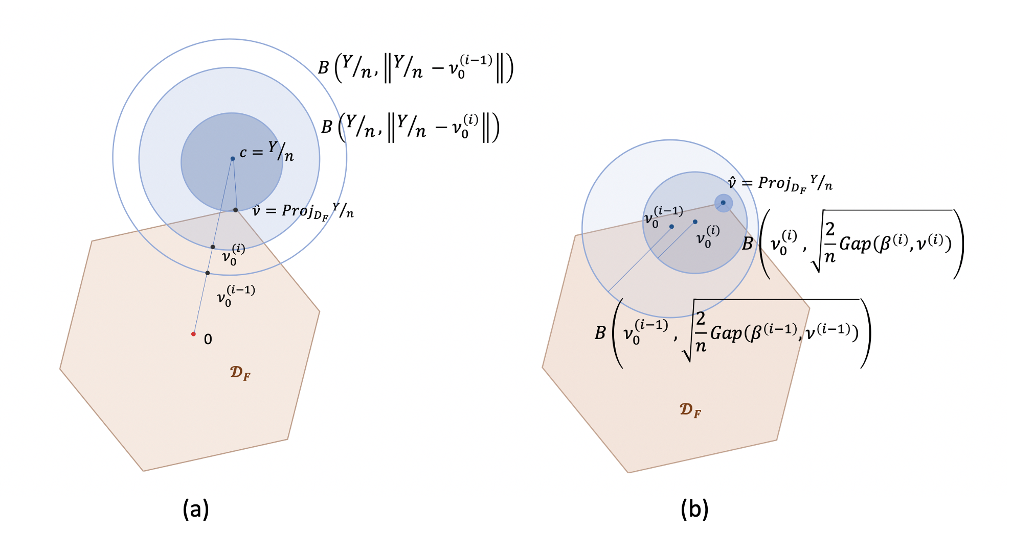
The idea behind dynamic screening [Bonnefoy et al. 2014] is to iteratively improve the dual feasible point $\nu_{0}$ during the coordinate descent updates. The residuals $Y-X\beta$ are updated at each iteration $i$ of the coordinate descent algorithm, and since the coordinate descent algorithm guarantees convergence, we have that

Recall that our SAFE rules depend on the feasible point $\nu_{0}$ through the radius of the spherical region on which we base the upper bounds : $B(c,r(\nu_{0}^{(i)}))=B\Big(\frac{Y}{n},\mathinner{\!\left\lVert\frac{Y}{n}-\nu_{0}^{(i)}\right\rVert}\Big)$. Also, recall that $\hat{\nu}=\mathrm{Proj}_{\mathcal{D}_{F}}\frac{Y}{n}=\min_{\nu\in\mathcal{D}_{F}}\mathinner{\!\left\lVert\frac{Y}{n}-\nu\right\rVert}^{2},$ $\hat{\nu}$ is the closest feasible point to the center $\frac{Y}{n}$. Hence, having $\nu_{0}$ closer to the optimal $\hat{\nu}$ reduces the radius of the sphere and ensures tighter upper bounds $\max_{\nu\in B(c,r)}|\nu^{T}G_{i}|$ and $\max_{\nu\in B(c,r)}|\nu^{T}(G_{i}\times E)|$ for $|\hat{\nu}^{T}G_{i}|$ and $|\hat{\nu}^{T}(G_{i}\times E)|$. This, in turn, ensures better SAFE rules that are able to discard more variables. By performing the SAFE rules screening not only at the beginning of each new iteration $\lambda_{k}=(\lambda_{1},\lambda_{2})_{k}$, but all along the iterations $i$ for the coordinate descent, we iteratively improve the estimate of $\hat{\nu}$ with $\nu_{0}^{(i)}$ and consequentially keep improving our SAFE rules.

The proposed procedure is the following: at each iteration $i$ of the algorithm use the current residuals $Y-X\beta^{(i)}$ to obtain a current estimate of the dual variable $\nu_{\mathrm{res}}^{(i)}=\frac{Y-X\beta^{(i)}}{n}$, naively project it onto the feasible set $\mathcal{D}_{F}$ and apply the SAFE rules (12). Figure 1(a) illustrates the iterative process of constructing the SAFE spherical regions. One concern is how expensive it is to compute the naive projection and the SAFE rules at each iteration, which we address in details in section 3.2.6.

However, there are clear disadvantages of our current choice of center $c=\frac{Y}{n}$ and radius $r=\mathinner{\!\left\lVert\frac{Y}{n}-\nu_{0}^{(i)}\right\rVert}$. Even when the dual feasible variable $\nu_{0}^{(i)}$ converges to the optimal value $\hat{\nu}$, the ball $B\big(\frac{Y}{n},\mathinner{\!\left\lVert\frac{Y}{n}-\hat{\nu}\right\rVert}\big)$ does not shrink around the dual optimal variable, since the radius does not converge to zero and the center is static, indicating that our upper bounds $\max_{\nu\in B\big(\frac{Y}{n},\mathinner{\!\left\lVert\frac{Y}{n}-\hat{\nu}\right\rVert}\big)}|\nu^{T}G_{i}|$ and $\max_{\nu\in B\big(\frac{Y}{n},\mathinner{\!\left\lVert\frac{Y}{n}-\hat{\nu}\right\rVert}\big)}|\nu^{T}(G_{i}\times E)|$ remain loose (Figure 1(a)). The Gap SAFE rules proposed by Fercoq et al. 2015 beautifully address the above disadvantages. We present the ideas behind the Gap SAFE rules and their application to the gesso model in the next section.

Denote the primal objective function for the gesso model as $P(\beta)$:

and the dual objective as $D(\nu)$:

The duality gap, denoted as $\mathrm{Gap}(\beta,\nu)$ is the difference between the primal and the dual objectives $\mathrm{Gap}(\beta,\nu)=P(\beta)-D(\nu).$ For the optimal solutions we have $P(\beta)\geq P(\hat{\beta})$ and $D(\nu)\leq D(\hat{\nu})$. By weak duality $D(\nu)\leq D(\hat{\nu})\leq P(\hat{\beta})\leq P(\beta)\implies\mathrm{Gap}(\beta,\nu)\geq 0.$ The duality gap provides an upper bound for the suboptimality gap $P(\beta)-P(\hat{\beta})$ as $P(\beta)-P(\hat{\beta})\leq P(\beta)-D(\nu)=\mathrm{Gap}(\beta,\nu)\leq\epsilon$. Therefore, given a tolerance $\epsilon>0$, if at iteration $t$ of the BCD algorithm we can construct $\beta^{(t)}$ and $\nu^{(t)}\in\mathcal{D}_{F}$ such that $\mathrm{Gap}(\beta^{(t)},\nu^{(t)})\leq\epsilon$, then $\beta^{(t)}$ is guaranteed to be a $\epsilon$-optimal solution of the primal problem. Note that in order to use the duality gap at iteration $t$ as a stopping criterion we need a dual feasible point $\nu^{(t)}\in\mathcal{D}_{F}$. We, again, utilize the naive projection method and obtain $\nu_{0}^{(t)}$.

Because $D(\nu)$ is a quadratic and strongly concave function with concavity modulus $n$ [Boyd and Vandenberghe 2004] we have: $D(\nu)\leq D(\hat{\nu})\ +\langle\nabla D(\hat{\nu}),\nu-\hat{\nu}\rangle-\ \frac{n}{2}\mathinner{\!\left\lVert\nu-\hat{\nu}\right\rVert}^{2},$

where the second inequality follows from weak duality and the optimality conditions for $\hat{\nu}$. Thus,

Gap SAFE rules work with the Euclidean ball with center $c=\nu^{(i)}_{0}$ and radius $r=\sqrt{\frac{2}{n}\mathrm{Gap}(\beta^{(i)},\nu^{(i)}_{0})}$, which we denote as $B_{\mathrm{Gap}}(c,r)$. This is a valid region since $\hat{\nu}\in B_{\mathrm{Gap}}(c,r)$ by (17). An important consequence of the above construction is that when $\beta^{(i)}\underset{i}{\longrightarrow}\hat{\beta}$, then $\nu_{0}^{(i)}\underset{i}{\longrightarrow}\hat{\nu}$ via the primal-dual link (6, 14) and $\mathrm{Gap}(\beta^{(i)},\nu_{0}^{(i)})\underset{i}{\longrightarrow}0$. Figure 1(b) illustrates that the dynamic approach discussed in the previous section in combination with the Gap SAFE rules very naturally results in improving the upper bounds $\max_{B_{\mathrm{Gap}}(c,r)}|\nu^{T}G_{i}|$ and $\max_{B_{\mathrm{Gap}}(c,r)}|\nu^{T}(G_{i}\times E)|$, since the radius of our new Gap ball converges to zero and the center converges to the dual optimal point. The Gap SAFE rules follow from substituting $r=\sqrt{\frac{2}{n}\mathrm{Gap}(\beta^{(i)},\nu^{(i)}_{0})}$ and $c=\nu^{(i)}_{0}$ in (12).

Massias et al. 2017 proposed to use a working set approach with the Gap SAFE rules to achieve substantial speedups over the state of art Lasso solvers, including glmnet. The working set strategy involves two nested iteration loops. In the outer loop, a set of predictors $W_{t}\subset\{1,..,p\}$ is defined, called a working set (WS). In the inner loop, the coordinate descent algorithm is launched to solve the problem restricted to $X_{W_{t}}$ (i.e. considering only the predictors in $W_{t}$).

We adopt the Gap SAFE rules we developed for the gesso model to incorporate the proposed working set strategy. Recall the SAFE rules we constructed in (12):

By simply rearranging the terms in the inequality we get:

Define the left-hand side of the above inequality as $d_{i}$. Note that our SAFE rules (12) are equivalent to $d_{i}>r$.

The idea is that $d_{i}$ now represents a score for how likely the predictor is zero or non-zero based on the Gap SAFE rules. Predictors for which $d_{i}$ is small are more likely to be non-zero and, conversely, predictors with larger values of $d_{i}$ are more likely to be zero up to the point when $d_{i}>r$ and the corresponding predictor is exactly zero by the SAFE rules. Here by predictor we mean the pair $(\beta_{G_{i}},\beta_{G_{i}\times E})$.

The proposed procedure is as follows: compute the initial number of variables to be assigned to the working set ($working\_set\_size$). Calculate $d_{i}$ and define the working set as the indices of the smallest $d_{i}$ values up to the value of $working\_set\_size$. Fit the coordinate descent algorithm on the variables from the working set only and check if we achieved an optimal solution via the duality gap for all of the variables. If not, increase the size of the working set, recalculate $d_{i}$ according to the new estimates obtained by fitting on a previous working set, and repeat the procedure. We increase the size of the working set by two each time.

Algorithm 1 presents the block coordinate descent algorithm and the stopping criterion we propose to use. Algorithm 2 describes the main steps of the working set strategy. To recapitulate, the main advantage of the algorithm is that we select variables that are likely to be non-zero and leave likely zeroes out so we do not have to spend unnecessary time fitting them. This approach can be thought of as an acceleration of the Gap SAFE rules.

In Algorithm 1 the dual feasible point required to determine the dual gap is calculated according to the naive projection method proposed in section 3.2.2. However, computing the naive projection is expensive, since it requires performing a matrix by vector product with a vector of length $n$ (sample size) and a matrix of size $n\times\text{length(working\_set)}$. The idea of an active set and adaptive max difference strategies is to reduce the number of times we have to evaluate check_duality_gap() function to ensure convergence.

Adaptive max difference strategy: In any iterative optimization algorithm, including coordinate descent, the convergence (stopping) criterion plays an important role. One of the most commonly used stopping criteria is based on the change in estimates between two consecutive iterations $t-1$ and $t$ (18). It is implemented in the glmnet package [Friedman et al. 2009], for example. The idea is that if the estimated coefficients do not change much from iteration to iteration it is likely the optimal solution has been reached:

However, in contrast to the duality gap stopping criterion, such heuristic rules do not offer control over suboptimality and it is generally not clear what value of $\epsilon$ is sufficiently small.

Although the heuristic convergence criterion based on the maximum absolute difference between consecutive estimates (18) does not control the suboptimality gap $P(\beta^{(t)})-P(\hat{\beta})$, it is very fast to compute, since $\mathinner{\!\left\lVert X_{i}\right\rVert}_{2}^{2}$ is pre-computed or normalized to be one. To reduce the number of times we check the convergence based on the duality gap criterion in Algorithm 1, we propose to use the criterion (18) as a proxy convergence criterion (Algorithm 3).

The proposed procedure is as follows: we initialize the tolerance for the max difference criterion as the tolerance we set for the duality gap convergence. We proceed by fitting the coordinate descent algorithm until we meet the max difference convergence criterion and then check the duality gap for the final convergence. If the duality gap criterion is not met, we decrease the max difference tolerance by a factor of 10 and proceed again. As a result, instead of checking the duality gap after each cycle of the coordinate descent algorithm, we wait until the proxy convergence criterion (which is very cheap to check) is met, and then check the duality gap criterion. By adaptively reducing the tolerance value of the proxy criterion we allow more coordinate descent cycles if needed, but carefully control the adaptive convergence to make as few checks as possible.

Active set strategy: The active set (AS) is a heuristic proposed by the authors of the glmnet package. The active set strategy tracks predictors updated during the first coordinate descent cycle and proceeds by fitting the coordinate descent algorithm only on those variables. The active set strategy combines naturally with our proposed adaptive max difference procedure since we also calculate the differences of the estimates on the consecutive iterations for our proxy convergence criterion. We believe that the max difference strategy we proposed in combination with the active sets can accelerate the state of art methods for fitting the standard Lasso as well. We summarize the main steps for both strategies in Algorithm 3, which is an optimized version of Algorithm 1.

To recapitulate, Algorithm 1 is the vanilla block coordinate descent algorithm, where each block in $\{1,...,p\}$, comprised of a main effect and its corresponding interaction, is updated until convergence without the use of any screening rule or heuristic. Algorithm 2 incorporates the Gap SAFE screening rules to the block coordinate descent algorithm in combination with the working set strategy. In the outer loop the variables in the working set are determined and in the inner loop the basic block coordinate descent Algorithm 1 is applied to the reduced set of variables. This achieves a lower run time. Algorithm 3 leverages additional heuristics to further accelerate the convergence on working sets by using active sets and the fast maximum absolute difference convergence criterion. Note that all the proposed improvements guarantee convergence to a global optimal solution since the final convergence criterion ensures that the duality gap for the full problem (including all the estimated variables) is within a given tolerance.

References

- Ayers and Cordell (2010) Ayers, K.L., Cordell, H.J. (2010). ”SNP selection in genome-wide and candidate gene studies via penalized logistic regression”, Genet Epidemiol, 34(8):879–891.
- Bhatnagar et al. (2018) Bhatnagar, S., Lovato, A., Yang, Y., Greenwood, C. (2018). ”Sparse Additive Interaction Learning”, bioRxiv 445304.
- Bien et al. (2013) Bien, J., Taylor, J., Tibshirani, R. (2013). ”A lasso for hierarchical interactions”, Ann. Statist. 41, no. 3, 1111–1141.
- Boyd et al. (2011) Boyd, S., Parikh, N., Chu, E., Peleato, B., Eckstein, J. (2011). ”Distributed optimization and statistical learning via the alternating direction method of multipliers”, Foundations and Trends in Machine Learning, 3(1):1–122.
- Bonnefoy et al. (2014) Bonnefoy, A., Emiya, V., Ralaivola, L., and Gribonval, R. (2014). ”A dynamic screening principle for the lasso”, In EUSIPCO.
- Boyd and Vandenberghe (2004) Boyd, S., Vandenberghe, L. (2011). ”Convex Optimization”, Cambridge University Press.
- Chang et al. (2000) Chang, B. D., Watanabe, K., Broude, E. V., Fang, J., Poole, J. C., Kalinichenko, T. V., and Roninson, I. B. (2000). ”Effects of p21Waf1/Cip1/Sdi1 on cellular gene expression: Implications for carcinogenesis, senescence, and age-related diseases”, Proc. Natl. Acad. Sci., 97(8), 4291–4296.
- Chipman (1996) Chipman, H. (1996). ”Bayesian Variable Selection with Related Predictors”, The Canadian Journal of Statistics, 24(1), 17–36.
- Cox (1984) Cox, D.R. (1984). ”Interaction”, International Statistical Review, 52(1), 1–24.
- Efroymson (1960) Efroymson, M.A. (1960). ”Multiple regression analysis”, Mathematical Methods for Digital Computers, Wiley, New York.
- El Ghaoui et al. (2012) El Ghaoui, L., Viallon, V., and Rabbani, T. (2012). ”Safe feature elimination in sparse supervised learning”, Pac. J. Optim., 8(4):667–698.
- Fercoq et al. (2015) Fercoq, O., Gramfort, A., and Salmon, J. (2015). ”Mind the duality gap: safer rules for the lasso”, In ICML, pages 333–342.
- Figueiredo et al. (2014) Figueiredo, J.C., Hsu, L., Hutter, C.M., Lin, Y., Campbell, P.T., Baron, J.A., Berndt, S.I., Jiao, S., Casey, G., Fortini, B., Chan, A.T., Cotterchio, M., Lemire, M., Gallinger, S., Harrison, T.A., Le Marchand, L., Newcomb, P.A,, Slattery, M.L., Caan, B.J., Carlson, C.S., Zanke, B.W., Rosse, S.A., Brenner, H., Giovannucci, E.L., Wu, K., Chang-Claude, J., Chanock, S.J., Curtis, K.R., Duggan, D., Gong, J., Haile, R.W., Hayes, R.B., Hoffmeister, M., Hopper, J.L., Jenkins, M.A., Kolonel, L.N., Qu, C., Rudolph, A., Schoen, R.E., Schumacher, F.R., Seminara, D., Stelling, D.L., Thibodeau, S.N., Thornquist, M., Warnick, G.S., Henderson, B.E., Ulrich, C.M., Gauderman, W.J., Potter, J.D., White, E., Peters, U. (2014). ”Genome-wide diet-gene interaction analyses for risk of colorectal cancer.”, PLoS Genet., 10(4).
- Friedman et al. (2007) Friedman, J., Hastie, T., Hoefling, H., Tibshirani, R. (2007). ”Pathwise Coordinate Optimization”, Ann. Appl. Stat., 2(1), 302–332.
- Friedman et al. (2010) Friedman, J., Hastie, T., Tibshirani, R. (2010). ”Regularization Paths for Generalized Linear Models via Coordinate Descent”, Journal of Statistical Software, 33(1).
- Friedman et al. (2009) Friedman, J., Hastie, T., Tibshirani, R. (2009). ”glmnet: Lasso and Elastic-Net Regularized Generalized Linear Models”.
- Gorgoulis et al. (2005) Gorgoulis, V. G., Pratsinis, H., Zacharatos, P., Demoliou, C., Sigala, F., Asimacopoulos, P. J., Papavassiliou, A. G., Kletsas, D. (2005). ”p53-Dependent ICAM-1 overexpression in senescent human cells identified in atherosclerotic lesions”, Laboratory Investigation, 85(4), 502–511.
- Hannum et al. (2013) Hannum, G., Guinney, J., Zhao, L., Zhang, L., Hughes, G., Sadda, S., Klotzle, B., Bibikova, M., Fan, J.-B., Gao, Y., Deconde, R., Chen, M., Rajapakse, I., Friend, S., Ideker, T., Zhang, K. (2013). ”Genome-wide methylation profiles reveal quantitative views of human aging rates”, Mol. Cell, 49 359–367.
- Haris, Witten and Simon (2016) Haris, A., Witten, D., Simon, N. (2016). ”Convex Modeling of Interactions With Strong Heredity”, J. Comput. Graph. Statist., 25:4, 981-1004.
- Jeck et al. (2012) Jeck, W.R., Siebold, A.P., Sharpless, N.E. (2012). ”Review: a meta-analysis of GWAS and age-associated diseases”, Aging Cell, 11(5):727–731.
- Kane, Emerson, and Weston (2013) Kane, M., Emerson, J., Weston, S. (2015). ”Scalable Strategies for Computing with Massive Data”, Journal of Statistical Software, 55(14), 1-19.
- Lim and Hastie (2015) Lim, M., Hastie, T. (2015). ”Learning Interactions Through Hierarchical Group-Lasso Regularization”, J. Comput. Graph. Statist., 24, 627–654.
- Liu et al. (2013) Liu, J., Huang, J., Zhang, Y., Lan, Q., Rothman, N., Zheng, T., Ma, S. (2013). ”Identification of gene–environment interactions in cancer studies using penalization”, Genomics, 102(4), 189–194.
- Massias et al. (2017) Massias, M., Gramfort, A., Salmon, J. (2017). ”From safe screening rules to working sets for faster lasso-type solvers”, 10th NIPS Workshop on Optimization for Machine Learning.
- Nelder (1977) Nelder, J.A. (1977). ”A Reformulation of Linear Models”, Journal of the Royal Statistical Society. Series A, 140(1), 48-77.
- Papaconstantinou et al. (2019) Papaconstantinou, J. (2019). ”The Role of Signaling Pathways of Inflammation and Oxidative Stress in Development of Senescence and Aging Phenotypes in Cardiovascular Disease”, Cells, 8, 1383.
- Qian et al. (2020) Qian, J., Tanigawa, Y., Du, W., Aguirre, W., Chang, C., Tibshirani, R., Rivas, M.A., Hastie, T. (2020). ”A Fast and Scalable Framework for Large-scale and Ultrahigh-dimensional Sparse Regression with Application to the UK Biobank”, bioRxiv 630079.
- Schoentgen et al. (2020) Schoentgen, F., Jonic, S. (2020). ”PEBP1/RKIP behavior: a mirror of actin-membrane organization”, Cell. Mol. Life Sci. 77, 859–874.
- Scholler et al. (2008) Scholler, N., Gross, J.A., Garvik, B. et al. (2008). ”Use of cancer-specific yeast-secreted in vivo biotinylated recombinant antibodies for serum biomarker discovery”, J. Transl. Med. 6, 41.
- Ternes et al. (2017) Ternes, N., Rotolo, F., Heinze, G., Michiels, S. (2017). ”Identification of biomarker-by-treatment interactions in randomized clinical trials with survival outcomes and high-dimensional spaces”, Biometrical Journal 59(4):685–701.
- Tibshirani (1996) Tibshirani, R. (1996). ”Regression shrinkage via the lasso”, J. R. Stat. Soc. Ser. B. Stat. Methodol. 58:267–288.
- Tseng (2001) Tseng, P. (2001). ”Convergence of a Block Coordinate Descent Method for Nondifferentiable Minimization”, J. Optim. Theory Appl., 109(3), 475–494.
- Wu et al. (2017) Wu, C., Jiang, Y., Ren, J., Cui, Y., Ma, S. (2017). ”Dissecting gene-environment interactions: A penalized robust approach accounting for hierarchical structures.”, Stat. Med., 37(3), 437–456.
- Wu et al. (2020) Wu, M., Zhang, Q., Ma, S. (2017). ”Structured gene‐environment interaction analysis.”, Biometrics, 76(1), 23–35.
- Yuan and Lin (2007) Yuan, M. and Lin, Y. (2007). ”Model selection and estimation in regression with grouped variables”, J. R. Stat. Soc. Ser. B. Stat. Methodol. 68(1), 49–67.
- Zou and Hastie (2005) Zou, H. and Hastie, T. (2005). ”Regularization and variable selection via the elastic net” J. R. Stat. Soc. Ser. B. Stat. Methodol. 67:301–320.
- Zhao et al. (2009) Zhao, P., Rocha, G., Yu, B. (2009). ”The composite absolute penalties family for grouped and hierarchical variable selection”, The Ann. Statist., 37(6A), 3468–3497.