Capturing Fingerprints of Conical Intersection: Complementary Information of Non-Adiabatic Dynamics from Linear X-ray Probes
Abstract
Many recent experimental ultrafast spectroscopy studies have hinted at non-adiabatic dynamics indicating the existence of conical intersections, but their direct observation remains a challenge. The rapid change of the energy gap between the electronic states complicated their observation by requiring bandwidths of several electron volts. In this manuscript, we propose to use the combined information of different X-ray pump-probe techniques to identify the conical intersection. We theoretically study the conical intersection in pyrrole using transient X-ray absorption, time-resolved X-ray spontaneous emission, and linear off-resonant Raman spectroscopy to gather evidence of the curve crossing.
Keywords:
X-ray Spectroscopy, Conical Intersections, Time-Resolved Spectroscopy, Quantum DynamicsI Introduction
Conical intersections 17; 4; 75, though once considered rare, govern the outcome of many of the photochemical reactions, according to modern photochemistry 12; 13; 14. They appear in a molecule when two or more potential energy surfaces cross and enable the possibility of electronic de-excitation without radiative emission. These non-radiative transitions result in the breakdown of the Born-Oppenheimer approximation. Consequently, the electronic and nuclear degrees of freedom are strongly coupled in the vicinity of the conical intersection. It is now well established that the conical intersections play a vital role in several photochemical processes such as photosynthesis 46, primary event of vision 70, photochemical formation of DNA lesions 16, and photochemistry of individual nucleobases 43. However, the direct experimental detection of conical intersections in molecular systems is still challenging. This is mainly because the energy gap between potential energy surfaces near the conical intersection decreases rapidly. Ultrashort pulses with adequate resolution in both energy and time domain are required to observe them.
With the advent of X-ray lasers, it is possible to probe such fast processes that occur on the timescale of femtoseconds and attoseconds using ultrafast pump-probe spectroscopy 18; 59; 74; 34; 9; 22; 63; 64; 23; 73; 3. It has been recently shown experimentally that attosecond transient absorption spectroscopy can aid the observation of non-adiabatic processes 29; 65; 44; 77. Time-resolved photo-electron spectroscopy 41; 6, and X-ray diffraction 7 have also been proposed to study the behaviour of system in the vicinity of a conical intersection.
Spectroscopic techniques that involve attosecond pulses provide a high resolution in the time-domain, and cover a broad range of frequencies, making them a promising tool to measure the rapidly varying energy gap that comes with conical intersections. However, their experimental availability can be a limiting factor.
In the following, we show theoretically how a combination of femtosecond based X-ray probe methods may be used to detect the non-adiabatic dynamics in a molecule. Our chosen example molecule, pyrrole, exhibits a conical intersection in the photodissociation pathway of the hydrogen atom. The branching ratio between the electronic states in the vicinity of the conical intersection is on the order of a few percent, making it a rather challenging example 19. The goal of the present work is to show that it is possible to locate a conical intersection even when there is an unbalanced branching of the electronic state population in its vicinity, using widely used femtosecond X-ray probe methods. A purely diabatic or purely adiabatic population transfer poses a challenge for spectroscopic X-ray techniques to identify the existence of the second electronic state involved in the conical intersection. Three different techniques have been employed to study the photo dynamics of pyrrole involving a conical intersection between ground and excited electronic state. The methods used here are as follows, time-resolved X-ray absorption spectroscopy, X-ray spontaneous emission spectroscopy and recently proposed technique, transient redistribution of ultrafast electronic coherence in attosecond Raman signals. We briefly introduce the features of the methods used in this manuscript in the following.
In the case when there is an unbalanced branching, one needs to look for the indirect signatures of a conical intersection to detect its occurrence. We construct the transient X-ray absorption spectroscopy spectrum using femtosecond X-ray probe-pulses to observe the change in transition dipole-moment in the vicinity of a conical intersection in pyrrole. Femtosecond pulses are sufficiently narrow in the frequency domain ( eV, as compared to attosecond pulses) to selectively probe the transitions which are distributed over a few electron volts. The intensity of the X-ray absorption spectroscopy signal depends on the valence-to-core transition dipole moments that the probe pulse is resonant with, as well as the population of the valence states. It is possible to construct X-ray absorption spectroscopy spectra using attosecond pulses, but it may contain signatures originating from other resonant valence-to-core transitions, further complicating the interpretation of the spectrum.
Time-resolved X-ray spontaneous emission spectroscopy 60; 45 does not solely depend upon the branching of the wave packet and may provide additional information about the curve crossing. In the X-ray spontaneous emission spectroscopy spectrum, the energy gap in the vicinity of the conical intersection may be observed directly independent of the population of the involved valence states and is expected to yield information about the shape of the potential energy surfaces involved. In time-resolved X-ray spontaneous emission spectroscopy, pyrrole is excited to a nitrogen 1s core-hole state, which is followed by the spontaneous emission of a photon. The 1s core-hole states of nitrogen have a lifetime of 7 fs 27; 24; 61, and the spontaneous emission takes place within this time period after excitation.
Probing the creation of electronic coherences in the vicinity of conical intersection provides a more direct signature of conical intersections. Several X-ray based spectroscopic techniques have been proposed theoretically to observe this phenomena 26; 11; 76; 6. One such scheme is transient redistribution of ultrafast electronic coherence in attosecond Raman signals 32; 28; 10, which is based on an off-resonant linear Raman process. In this scheme, a hybrid probe-pulse sequence is used instead of a single probe pulse to construct the signal where the redistribution of photons maps out the time varying energy gap via the Raman shift. Transient redistribution of ultrafast electronic coherence in attosecond Raman signals is only sensitive to the coherences and is thus expected to yield accurate information about the passage through the conical intersection. However, to obtain the maximum intensity in the signal, a balanced branching at the conical intersection is required. The result from transient redistribution of ultrafast electronic coherence in attosecond Raman signals signal can be considered confirmation for the other two methods. The use of hybrid pulses in transient redistribution of ultrafast electronic coherence in attosecond Raman signals and homodyne detection scheme makes it experimentally more challenging, whereas X-ray absorption spectroscopy and X-ray spontaneous emission spectroscopy have been used successfully earlier in experiments to study photochemical processes 1; 30.
We show that the three methods deliver complementary information that can be used to observe the direct (generation of vibronic coherence and state resolved spectra) and indirect (change in the transition dipole moments) effects of a conical intersection between two states in the pyrrole molecule. The paper is structured as follows: section II presents the details of the system used for the signal calculations. In section III, the analytical expressions for spectroscopic signals and Hamiltonian for the various pump-probe methods are discussed. Section IV contains the details about the software and programs used to carry out the simulations. In section V, spectra calculated using different pump-probe methods are presented along with the discussion. Finally, the main conclusions drawn by comparing the results from used methods are presented in section VI.
II Model
II.1 Photochemistry of pyrrole
Pyrrole is a nitrogen-containing five-membered heterocyclic aromatic compound, which has been used extensively as a model system for exploring non-adiabatic dynamics 48; 49; 50; 51; 52; 53; 19. The low-lying bright states of pyrrole emerge around 6 eV 54; 55. It has been challenging to assign the corresponding peaks in ultra violet absorption spectrum. This is mainly due to the high density of energy levels lying around the bright states 56; 57.
The ultra violet-induced photochemistry of pyrrole involves NH detachment process through the manifold of four lowest singlet excited states, 1A2(), 1B1(), 1B2(), and 1A1() 47; 19. The two states have been assigned to the above-mentioned absorption bands around 6 eV. The molecules in these bright states undergo non-radiative decay to the states along the out-of-plane ring deformation coordinate 58. The latter states have been found to be repulsive along the NH stretching mode 49; 68; 69. The ring deformation mechanism was also shown to be feasible on the states 58. Along the dissociation process, the ground state energy increases and forms a CI between and states 49. The nature of the orbital was also shown to be varied during the detachment process. At the Franck-Condon geometry, it is of 3s Rydberg type which changes to valance upon NH stretching and eventually becomes a 1s orbital of the hydrogen atom. This Rydberg-to-valance orbital transformation rationalises the presence of the dissociation barrier on the states 49. The photodissociation dynamics of pyrrole involving /(1A2 and 1B1) CIs have been theoretically investigated by Domcke and co-workers 19. The study employs the vertical excitation model and simulates the time-dependent dynamics of pyrrole on each state separately. Recently, optical cavities have been found to be hugely influencing the photolysis reaction dynamics in the (1B1) state 36. The present work considers the photodynamics of pyrrole in the (1B1) state, referred to as just in the rest of the paper, as a model for the study. We have employed a simplified model by considering only the stretching coordinates corresponding to the NH bond. This reduced dimensionality model has been found to be describing the photofragmentation features of pyrrole qualitatively 19.
The main objective of the paper is to show how femtosecond based X-ray probe methods can be used to detect the CIs in molecular systems. Therefore, we include only and states, and the vibronic couplings of them with the other valance excited states have been neglected. These additional vibronic interactions 66; 67; 68; 69 and the other molecular modes like out-of-plane ring deformation 58, as mentioned above, may also play a role in describing the dissociation dynamics of pyrrole. Our model does not consider these effects. The treatment of all these couplings in an extended molecular mode space would be necessary for a fully quantitative description of the time-dependent photodissociation dynamics of pyrrole 66; 67; 68; 58; 69.
A detailed discussion on the potential energy surfaces of valance states employed in the current work can be found in a recent study investigating the cavity-modified dynamics of pyrrole 36. We provide the details very briefly here. Previous theoretical studies have established that the hydrogen elimination reaction dynamics in the state involves hydrogen in-plane and out-of-plane detachment motions 19; 36. These coordinates, which will be denoted as and refer to the tuning and coupling coordinates, respectively. The computed potential energy surfaces along the two reaction coordinates have been used to construct various spectroscopic signals from the quantum dynamics simulations. The valence states are considered to be in the diabatic basis. When the wave packets reach the conical intersection, there is a diabatic population transfer (around of population in excited state), mediated by the diabatic coupling between the states.

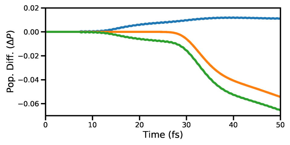
The wave-packets on the state potential energy surface arrive in the vicinity of conical intersection at around and then starts to branch into , which can be seen in the population difference curves shown in Fig. 1 for state (blue curve) and state (green curve). The population difference for a particular state is calculated by subtracting the maximum population from the population at each time instance after the end of pump-pulse. The total population (orange curve) remains constant until the wave-packets reaches the boundary of the potential energy surface and gets absorbed by perfectly matched layer 42. To analyze the behavior of the system near conical intersection, we use five core-hole states, which correspond to Nitrogen orbital. The 1D strips of the potential energy surfaces are shown in Fig. 2. The two valence states are denoted by and while the lowest core-hole state is denoted by .
II.2 Preparation of the system
A pump-probe scheme is used in the construction of the signals, as shown in Fig. 3. An ultra violet pump-pulse is used to prepare the system by exciting it from the ground state () to the valence excited state () of the molecule.
The interaction of the molecule with the pump-pulse is included in the initial Hamiltonian, and the system after the interaction is called the prepared system. The Hamiltonian of the corresponding system can be written as,
| (1) |
where is the molecular Hamiltonian for the valence states, is the Hamiltonian which considers the effects of pump-pulse on the molecule under the dipole approximation. The molecular Hamiltonian and the interaction with ultra violet pump-pulse reads:
| (2) | ||||
| (3) |
In the Hamiltonian matrix in Eq. 2, and represent the kinetic energy operator and potential energy surface for a particular electronic state, respectively, and represents the diabatic couplings between the states and . The reduced mass is used in the kinetic energy operator , with being the gradient operator with respect to the reaction coordinates and . The , , and depend on the two reaction coordinates, and . In the Hamiltonian describing the interaction with the pump, and represent the transition dipole moments between and states. represents the electric field strength of pump-pulse, is the carrier frequency of the pump-pulse and is the Gaussian envelope of the laser pulse.

III Spectroscopic Signals
The expressions for the spectroscopic signals are discussed here, along with the modifications in Hamiltonian of the system. The electric field’s effects from the pump pulse are calculated without any further approximation by including it in the system Hamiltonian (called prepared system) for all pump-probe signals.
III.1 X-ray Absorption Signal
In transient X-ray absorption spectroscopy, the absorption of an X-ray pulse, the interaction with a valence-to-core transition is recorded. The obtained spectrum contains information about the possible transitions. We note that photoelectrons can also be generated in a competing process. However, we neglect all the competing pathways and focus on the X-ray absorption spectroscopy signal. Here we have included the pump pulse in the Hamiltonian which creates the initial state ( in Eq. 1). The interaction with the probe pulse is treated with time dependent perturbation theory. The total Hamiltonian can be written as follows,
| (4) |
where is the interaction Hamiltonian representing the interaction between probe-pulse and the prepared system. Under the rotating wave approximation, the time-dependent interaction Hamiltonian is
| (5) |
with being the transition dipole operator for describing the valence-to-core transition and is the electric field operator of the X-ray modes. The field state is considered to be a coherent state initially.

The signal for the X-ray absorption spectroscopy spectrum is defined as the integrated rate of change of the number of photons as a function of the absorption frequency and a pump-probe delay , and can be expressed as follows,
| (6) |
with being the photon number operator for the th field-mode. The interaction Hamiltonian, in Eq. 4, appears in the signal expression as a consequence of the probe-pulse electric field . The signal expression is then obtained by treating as the time-dependent perturbation. The expression then reads 6; 20; 40; 33,
| (7) | ||||
where is the carrier frequency of the X-ray probe-pulse, is its Gaussian envelope, and is the frequency of the th mode of the probe, and is the correlation function which contains the information about the interaction between the probe-pulse and the system, for time instances and as shown in Fig. 4.
| (8) |
where represents the superposition of the wave functions that evolve on valence states of the molecule according to the prepared-system Hamiltonian . Note that Eq. 7 describes both, absorption and stimulated emission according to the diagrams in Fig. 4.
III.2 X-ray Spontaneous Emission Signal

The probe pulse of a particular center frequency is used to excite the system from the valence states to the core-hole states. The core-hole states of Nitrogen in pyrrole have a lifetime of 7 fs 27; 24; 61 and hence spontaneous emission back to the valence states occurs on this time scale. To keep the computational effort tractable and stay within Hilbert space, we introduce the core-hole lifetime as an empirical parameter. Here we also neglect the photoionization due to the X-ray probe pulse as well as the subsequent Auger decay 15; 72; 5 and instead solely focus on spontaneous emission process. Note that the Auger process can be a dominant decay channel for relaxation from core excited states in light elements 25; 71. The total Hamiltonian for constructing the X-ray spontaneous emission spectroscopy signal is similar to the Hamiltonian in Eq. 4. The difference is that now both the pump and probe pulses are included in the initial Hamiltonian, and the subsequent spontaneous emission process is treated with perturbation theory. The molecular Hamiltonian, the pump interaction, and probe interaction are expressed as follows:
| (9) |
| (10) |
| (11) |
The notations in the molecular and pump field Hamiltonians are identical to the notation used in Eq. 2 and Eq. 3 with being a core-hole state. In the probe field Hamiltonian matrix , ’s represents the dipole moment between the valence ( and ) and core-hole () states, 2.06 V/m is the electric field strength of the probe pulse, is the carrier frequency of probe-pulse in X-ray regime, and is the Gaussian envelope of the probe-pulse. The field operator of the spontaneously emitted photons takes the following form,
| (12) |
where is the quantization volume, and represents the frequency of the spontaneously emitted photon. The X-ray spontaneous emission spectroscopy signal is defined as the integrated rate of change of the number of photons as a function of the emission frequency and the pump-probe delay . The signal expression then reads 35,
| (13) | ||||
where , with 7 fs, is the decay rate for the core-hole states and is the correlation function corresponding to the diagram shown in Fig. 5. The integral over the frequency is skipped in the final signal calculations as it is the variable for the frequency resolved detection. The two-time correlation function can be written as follows,
| (14) |
where represents the state which is populated at the pump-probe delay by X-ray pulse.
III.3 transient redistribution of ultrafast electronic coherence in attosecond Raman signals

In contrast to X-ray absorption spectroscopy and X-ray spontaneous emission spectroscopy, transient redistribution of ultrafast electronic coherence in attosecond Raman signals is a technique which is only sensitive to the vibronic coherences generated in the molecule. It uses a hybrid, off-resonant probe-pulse sequence. The signal consists of a Stokes and anti-Stokes type signal generated due to the redistribution of the photons between different modes. The transient redistribution of ultrafast electronic coherence in attosecond Raman signals spectrum is centered at the difference of the carrier frequencies of the hybrid probe pulses. The Raman shift indicates the energy difference between the involved valence states. Here we assume that the probe pulses have the same carrier frequency. The transient redistribution of ultrafast electronic coherence in attosecond Raman signals signal, which is constructed by perturbative treatment of the hybrid probe pulses, is represented by the following expression 32,
| (15) | ||||
where is the linear combination of the valence-states wave function at the pump-probe delay , is the Raman frequency, and are the two probe pulses respectively, and represents the polarizability tensor of the molecule 8:
| (16) |
where each element , with represents the directions of polarization. Each tensor element is expanded in the basis of the valence states:
| (17) |
Every element , with representing the initial and final valence states, depends on the nuclear coordinates and , and the frequency of the probe-pulses 8:
| (18) |
where is the resonance frequency between the core-hole state and the valence state .
The matrix from Eq. 17 becomes non-Hermitian when Eq. 18 is used. Here we make the assumption that the energy difference between the valence states is small compared to and the off-diagonal elements can be written as the average: . The new polarizability matrix, that is used in the calculations, then reads:
| (19) |
IV Methods
The ground state minimum structure of pyrrole, optimized at DFT/B3LYP/aug-cc-pVDZ level of theory, has been used as the reference geometry for computing the potential energy surfaces. A rigid 2D-potential energy surface scan has been performed by employing the complete self-consistent field (CASSCF) method along with the aug-cc-pVDZ basis set. Three states have been included in the state-averaged CASSCF for calculating the potential energy surfaces corresponding to the electronic valance states. The active space is comprised of seven orbitals (5 -orbitals of ring and a pair of -orbitals of NH bond) and 8 electrons. To compute the core excited state energies involving the electronic transition from the 1s-orbital of nitrogen atom, complete active space configuration interaction (CASCI) method has been used. The prior-mentioned 3-state averaged CASSCF wave function, and the corresponding orbitals have been utilized to generate the configurations in the CASCI method. The diabatic potential energy surfaces have been obtained using the quasi-diabatization procedure as implemented in MOLPRO-2019. The corresponding transformation matrix has been used to transform the dipole moments from adiabatic to diabatic basis. The program package MOLPRO-2019 37; 38 has been used for the electronic structure calculations.
The correlation functions in Eqs. 8, 14, and 15 have been calculated by a direct propagation simulation protocol 31. The wave packet dynamics have been calculated with our in-house software QDng. The Arnoldi method 2 was used to propagate the wave functions. The potential energy surfaces and the numerical wave functions are represented on a grid with dimensions . A perfectly matched layer is used to absorb the wave packets at the boundary of the numerical grid. The second derivative with respect to the reaction coordinates is calculated using the Fourier transform method. For all the propagations, a time step size of 50 as has been used. Since the lifetime of nitrogen 1s core-hole states is 7 fs, the time-evolution of the core-hole states in the X-ray spontaneous emission spectroscopy signal is done until 12.2 fs.
V Results and Discussion

The X-ray absorption spectroscopy signal is calculated by solving Eq. 7 for the core-hole states shown in Fig. 2. The state is energetically eV apart from nearest core-hole state in the vicinity of the conical intersection and thus the X-ray absorption spectroscopy signal is constructed only for the state. This can be used to distinguish the various features in the spectrum. The X-ray pulse has a finite width in the energy domain and thus the signal can be expected to show sharp features. Using an appropriate pulse-width and center-frequency of the X-ray pulse, it is possible to probe absorption bands belonging to different energy regimes as shown in Fig. 2. The signals are shown in Fig. 7 for three different X-Ray probe center frequencies, corresponding to transitions A, B and C in Fig. 2. Note that, when all the core-hole states are considered for the signal construction, the transitions corresponding to A and B for state will be resonant with transitions from other core-hole states as well. The X-ray absorption spectroscopy spectrum shown in Fig. 7(a) corresponds to the transition from state to state in the energy regime denoted by A in Fig. 2. The signal has almost constant intensity for all measured time-delays, while small variations in intensity originate from the pump pulse and the unbalanced branching ratio near the conical intersection. We note that the signal shows similar features as the attosecond transient absorption spectroscopy spectrum recorded for the carbon K-edge in to study the conical intersection between the and states 77. This signal has higher intensity compared to signals corresponding to the transitions B and C in Fig. 2. The reason being the population residing at the local minima of state, as shown in Fig. 2, is higher than the population transferred to the state by the pump pulse. Hence the intensity of signal in Fig. 7(a) is used as a reference for signals corresponding to other energy regions. The signal shown in Fig. 7(b) correspond to the transition B in Fig. 2 and it has highest intensity when pump-pulse is about to vanish and the intensity decreases when the wave packets starts to move away from the Franck-Condon point. The steady decrease in the intensity after some time indicates the presence of a local minima in the state. A certain amount of population is trapped in that minima that continues to leak over time.

Figure 7(c) indicates that the absorption is taking place near the conical intersection: the signals appears when the wave-packets on the state arrive in the vicinity of the conical intersection and it vanishes when the wave-packets move past the conical intersection region and move out of resonance with the probe-pulse. The transition from state to near the conical intersection has a significantly higher intensity compared to transition between same states in the Franck-Condon region (transition B in Fig. 2), and it can be observed by comparing Fig. 7(b) and Fig. 7(c). The increase in the intensity of signal near the conical intersection indicates that the transition dipole-moment between the involved states increases in the vicinity of the conical intersection. The fact that there are parts of the wave packets retained in the local minimum at the Franck-Condon of the state supports the conclusion about increase in transition dipole-moment around conical intersection. There is an increase in the intensity of the signal in Fig. 7(a), between 5 and 20 fs and around 40 fs, when the wave packets pass through the conical intersection. It is a result of the transfer of low energy wave-packets from to the state near conical intersection, that return to the minima of state. These vibrationally excited wave packets oscillate in the bounded region of the potential. Note that it is not possible to observe the change in the nature of the orbital along the dissociation coordinate in XAS spectrum. The X-ray probe frequency required to probe the transformation region is almost resonant with the absorption frequency of CI region. As a result the XAS signal from CI region dominates the XAS signal from the Rydberg-to-valence transformation region.


The X-ray absorption spectroscopy spectra shown in Fig. 8 contains the contributions from five core-hole states. The non-adiabatic couplings between the core-hole states, which have avoided crossings, are not included in the calculations. The avoided crossings are spatially well separated from the conical intersection between the valence states and thus it is expected that these crossings do not significantly alter the spectrum. When all five core-hole states (shown in Fig. 2) are used to construct the X-ray absorption spectroscopy signal, multiple valence-to-core transitions can be resonant with the same probe-pulse center-frequency. The transition C in Fig. 2 has the lowest energy and it is the only transition resonant with the probe pulse with a center frequency 404 eV. The number of resonant transitions increases by further increasing the carrier frequency.
The X-ray absorption spectroscopy signal corresponding to the transitions taking place in the vicinity of conical intersection is shown in Fig. 8(c). Due to the resonance condition, signal in Fig. 8(c) has the same shape as the signal for a single core-hole state has in Fig. 7(c). The transition corresponding to the Franck-Condon region for the state is resonant with the transition between the state and the conical intersection region, and hence there is increase in intensity of the signal between and in Fig. 8(b). The overlap of multiple signals can also be seen in the Fig. 8(a) which correspond to the absorption from the state’s local minimum. Since the intensity of the signal in Fig. 8(a) is used as a reference for other (Fig. 8(b) and (c)) signals, the spectrum in Fig. 8(c) has a lower intensity than the signal in Fig. 7(c). Apart from the change in peak intensity for absorption corresponding to 412 eV in Fig. 7 and 8, there is a noticable difference between the shape of the signals as well. The increase of intensity in the X-ray absorption spectroscopy spectrum in Fig. 8(c) at around 8 fs, can be interpreted as an arrival of the wave packet in the conical intersection region.
The X-ray spontaneous emission spectroscopy spectrum can be used to complement the findings from the X-ray absorption spectroscopy signal and to observe the energy gap between the valance states directly. The X-ray spontaneous emission spectroscopy spectrum is constructed by solving Eq. 13. For the sake of clarity, the X-ray spontaneous emission spectroscopy signals are constructed for both and states separately. In the simulated spectra, the contribution to the total signal from each state can be evaluated.
The spectrum shown in Fig. 9(a) corresponds to the signal of the final state and it gets stronger when the wave packets approach the conical intersection. The signal decays when the location of the wave packets is not resonant anymore with the probe pulse. This behavior follows a trend between 5 fs and 20 fs which corresponds to the blue curve in the Fig. 9(c) representing the separation between the state and the state as a function of a reaction coordinate. The signal that corresponds to the state is shown in Fig. 9(b) and the increase and decrease in intensity over the time shows a similar behavior as in the case of the state.
The change in intensity as a function of emission frequency and time delay in X-ray spontaneous emission spectroscopy spectra can be understood as follows: The spatial position of the wave packets on a potential energy surface relates them to a possible transition frequency for a particular state. If the energy of an excitation pulse is resonant or close to resonance for that transition frequency, the excitations will be maximum which would result in higher emission. Since the energy of the X-ray pulse is 403.3 eV, the signal will have the highest intensity when the wave packets reach the region before the conical intersection which has resonance frequency of around 404 eV. For a specific delay, the strength of the signal would depend upon the transition dipole moment between the valence and core-hole states. Out of the two valence states, the state has higher amplitude of transition dipole-moment to the state and hence will have higher intensity of X-ray spontaneous emission spectroscopy signal.
As can be seen in Fig. 9(c), the separation between the state and the state is almost constant (represented by orange curve) and a similar feature is found in the X-ray spontaneous emission spectroscopy spectrum in Fig. 9(b). This indicates that the X-ray spontaneous emission spectroscopy may be able to project the relative shapes of the potential energy surfaces of involved states. The total X-ray spontaneous emission spectroscopy spectrum which includes both the valence states is shown in the Fig. 10. The region shown in the red box corresponds to the state before the conical intersection, and the region shown in the black box corresponds to the same state but after the conical intersection. The signal in the black box starts to develop around 10 fs, which matches the time when the system reaches the conical intersection as predicted by the X-ray absorption spectroscopy signal in Fig. 7. The valence states can be seen to approach each other before 10 fs and move apart subsequently.

Assuming that the transition dipole moments between the two valence states and the core-hole states are comparable to each other, the X-ray spontaneous emission spectroscopy signal can be used to detect the two potential energy surfaces approaching each other before the conical intersection and move apart after the conical intersection. The only necessary condition is that the energy of the X-ray pulse should be resonant with the core-hole states in conical intersection region.
We now discuss the transient redistribution of ultrafast electronic coherence in attosecond Raman signals spectrum. Figure 11 shows the transient redistribution of ultrafast electronic coherence in attosecond Raman signals spectrum, which has been calculated using Eqs. 15 and 19. The transient redistribution of ultrafast electronic coherence in attosecond Raman signals spectra for the and components of the X-ray polarizability tensor, and are shown separately in Figs. 11(a) and (b) along with the sum of both components in Fig. 11(c). Note that the sum spectrum corresponds to a rotational averaged spectrum, which would be observed in a gas-phase experiment. The spectrum corresponding to is not shown here because it is five orders of magnitude weaker. The transient redistribution of ultrafast electronic coherence in attosecond Raman signals spectrum without the ultra violet pump pulse has been subtracted from that of the prepared system with the ultra violet pump pulse to remove the contribution from ground state vibrational Raman transitions.
The peak before 5 fs stems from the vibrational coherences created by the pump-pulse. At around 5-10 fs the wave packet reaches the conical intersection region where the non-adiabatic couplings come into effect. Inspection of Figs. 11(a) and (b) shows an increase in intensity, indicating a build up of coherence.
Between 10 and 30 fs the effects of the conical intersection can be seen in the spectrum. Both components in Figs. 11(a) and (b) show an increase in intensity. The component in Fig. 11(a) peaks between 10 and 20 fs and falls off at later times. The component in Fig. 11(b) also peaks between 10 and 20 fs but has another strong peak at 30 fs. This increase can be explained as the build up in coherence as well as an increase in polarizability. The component of the polarizability of the peaks before the conical intersection (at short NH bond distances) and goes to nearly zero after the wave packet has passed through the conical intersection. The component shows the opposite behavior: it is near zero before the wave packet reaches the conical intersection and peaks at larger NH bond distances. This explains the peak in Fig. 11(b) at 30 fs.

The Stokes and anti-Stokes patterns of the spectra for the and components are out of phase, leading to a partial cancellation of the signal in Fig. 11(c). However, the oscillation patterns still have the same period. The strength of the transient redistribution of ultrafast electronic coherence in attosecond Raman signals signal depends on the magnitude of the matrix elements of the polarizability operator (see Eq. 19) along with the magnitude of the coherence generated. The diagonal elements of the polarizability operator constitute the vibrational coherence, while the off-diagonal elements constitute the electronic coherence in the spectrum. The transient redistribution of ultrafast electronic coherence in attosecond Raman signals spectra are constructed separately for the vibrational coherence and the electronic coherence to compare the effect on the overall signal. The transient redistribution of ultrafast electronic coherence in attosecond Raman signals signal corresponding to electronic coherence is shown in Fig. 12(b), and it has a maximum intensity around 10 fs which is the time-instance when the wave packets start reaching the conical intersection. The transient redistribution of ultrafast electronic coherence in attosecond Raman signals signal corresponding to the vibrational coherence is shown in Fig. 12(a). Inspection of the polariziabilty matrix elements (see Eq. 19) also reveals that the diagonal elements are 2 times larger than the off-diagonal elements. Thus, the electronic coherences contribute significantly less than the vibrational coherences to the overall transient redistribution of ultrafast electronic coherence in attosecond Raman signals signal. Hence, the key signature of the conical intersection, i.e. electronic coherence generation, is not clearly visible in the transient redistribution of ultrafast electronic coherence in attosecond Raman signals signal for pyrrole. Note that the vibrational and electronic degrees of freedom are strongly mixed in the direct vicinity of the conical intersection and thus one can not clearly distinguish between vibrational and electronic coherences.
After 30 fs the intensity of the signal decreases due to the dissociation. Note that this decay is mainly caused by absorption of the wave packet at the grid boundary (see Fig. 1). In these particular examples of the transient redistribution of ultrafast electronic coherence in attosecond Raman signals spectrum does not show the expected frequency resolution and time evolution of the energy gap between the valence states can not be visualized. This is mainly due to the choice of pulse parameters which are necessary to resolve the spectral features in the time domain.
VI Conclusion
We have studied the conical intersection in pyrrole using three different spectroscopy techniques, namely X-ray absorption spectroscopy, X-ray spontaneous emission spectroscopy, and transient redistribution of ultrafast electronic coherence in attosecond Raman signals. A set of transient X-ray absorption spectroscopy spectra was constructed by selecting the dominant states involved in the non-adiabatic dynamics (, ) and the transitions to the first nitrogen 1s core hole state. We could show that the signature of the conical intersection in the spectrum consists of a resonance and an increase in signal intensity: For the lowest probe energy, the probe becomes resonant with the first core-hole state and a peak appears in the spectrum when the wave packet reaches the conical intersection region. The transition dipole moment peaks in the vicinity of the conical intersection leading to an increased absorption indicating the time it takes for the wave packet to reach the conical intersection, allowing to narrow down the timing further. Due to the unbalanced branching of the wave packet at the conical intersection, we see mainly the signature of the state in spectrum.
The time-resolved X-ray spontaneous emission spectroscopy spectrum was constructed using an X-ray probe-pulse, which has a frequency that is resonant with the valence-to-core transition corresponding to the conical intersection region. The state and the state have a similar shape and thus a constant energy difference in the vicinity of conical intersection. Consequently, the spontaneous emission peaks at a rather constant photon energy. In contrast to the X-ray absorption spectroscopy spectrum, the branching ratio at the conical intersection is not a decisive factor. The spontaneous decay from the nitrogen 1s core hole state has a similar transition moment to and the state. As a result, one can now see a signature of the curve crossing in the X-ray spontaneous emission spectroscopy spectrum.
For the third technique we have constructed the transient redistribution of ultrafast electronic coherence in attosecond Raman signals signal. Here we explicitly probe the vibronic coherences that are generated in the molecule by means of a linear off-resonant Raman process. The transient redistribution of ultrafast electronic coherence in attosecond Raman signals signal depends on the X-ray transition polarizability and the magnitude of the electronic and vibrational coherences of the excited system. The simulated spectrum displays peaks between 10 fs and 20 fs which hint at non-adiabatic dynamics due to the conical intersection. The spectra originating from the two polarizability tensor components are out of phase and the overall signal is diminished. The spectral features correlate with the signatures of the X-ray absorption spectroscopy and X-ray spontaneous emission spectroscopy spectra putting the passage through the conical intersection consistently between 10 fs and 20 fs. We note that the transient redistribution of ultrafast electronic coherence in attosecond Raman signals spectrum is dominated by the vibrational coherences and the increase of the polarizability near the conical intersection rather than the electronic coherences.
In conclusion, we have shown that the existence of a conical intersection in a molecule and its temporal appearance can be identified by a combination of multiple methods. Each technique on its own may deliver a spectrum that could potentially be difficult to interpret. The presented techniques probe different properties of the molecule and thus their combination gives a more complete picture. We also note that the combination is also potential strategy to bypass the high demand on the pulse bandwidth to map out the rapidly changing energy near the conical intersection. The pulses used in our simulations were longer than 1 fs thus explicitly avoiding attosecond pulses.
Acknowledgements
Support from the Swedish Research Council (Grant VR 2018-05346) is acknowledged.
Data Availability
The data is available on request from the authors.
References
- [1] Cited by: §I.
- [2] Cited by: §IV.
- [3] Cited by: §I.
- [4] Cited by: §I.
- [5] Cited by: §III.2.
- [6] Cited by: §I, §I, §III.1.
- [7] Cited by: §I.
- [8] Cited by: §III.3, §III.3.
- [9] Cited by: §I.
- [10] Cited by: §I.
- [11] Cited by: §I.
- [12] Cited by: §I.
- [13] Cited by: §I.
- [14] Cited by: §I.
- [15] Cited by: §III.2.
- [16] Cited by: §I.
- [17] Cited by: §I.
- [18] Cited by: §I.
- [19] Cited by: §I, §II.1, §II.1, §II.1.
- [20] Cited by: §III.1.
- [21] Cited by: Figure 4.
- [22] Cited by: §I.
- [23] Cited by: §I.
- [24] Cited by: §I, §III.2.
- [25] Cited by: §III.2.
- [26] Cited by: §I.
- [27] Cited by: §I, §III.2.
- [28] Cited by: §I.
- [29] Cited by: §I.
- [30] Cited by: §I.
- [31] Cited by: §IV.
- [32] Cited by: §I, §III.3.
- [33] Cited by: §III.1.
- [34] Cited by: §I.
- [35] Cited by: §III.2.
- [36] Cited by: §II.1, §II.1.
- [37] Cited by: §IV.
- [38] Cited by: §IV.
- [39] Cited by: Figure 4.
- [40] Cited by: §III.1.
- [41] Cited by: §I.
- [42] Cited by: §II.1.
- [43] Cited by: §I.
- [44] Cited by: §I.
- [45] Cited by: §I.
- [46] Cited by: §I.
- [47] Cited by: §II.1.
- [48] Cited by: §II.1.
- [49] Cited by: §II.1, §II.1.
- [50] Cited by: §II.1.
- [51] Cited by: §II.1.
- [52] Cited by: §II.1.
- [53] Cited by: §II.1.
- [54] Cited by: §II.1.
- [55] Cited by: §II.1.
- [56] Cited by: §II.1.
- [57] Cited by: §II.1.
- [58] Cited by: §II.1, §II.1.
- [59] Cited by: §I.
- [60] Cited by: §I.
- [61] Cited by: §I, §III.2.
- [62] Cited by: Figure 2.
- [63] Cited by: §I.
- [64] Cited by: §I.
- [65] Cited by: §I.
- [66] Cited by: §II.1.
- [67] Cited by: §II.1.
- [68] Cited by: §II.1, §II.1.
- [69] Cited by: §II.1, §II.1.
- [70] Cited by: §I.
- [71] Cited by: §III.2.
- [72] Cited by: §III.2.
- [73] Cited by: §I.
- [74] Cited by: §I.
- [75] Cited by: §I.
- [76] Cited by: §I.
- [77] Cited by: §I, §V.
References
- (1) Wolfgang Domcke, David R Yarkony, and Horst Köppel. Conical Intersections. World Scientific, 2011.
- (2) Michael Baer. Beyond Born-Oppenheimer: electronic nonadiabatic coupling terms and conical intersections. John Wiley & Sons, 2006.
- (3) David R. Yarkony. Conical Intersections: Diabolical and Often Misunderstood. Accounts Chem. Res., 31(8):511–518, 1998.
- (4) M. Klessinger and J. Michl. Excited States and Photochemistry of Organic Molecules. VCH, 1995.
- (5) M. A. Robb, F. Bernardi, and M. Olivucci. Conical intersections as a mechanistic feature of organic photochemistry. Pure and Applied Chemistry, 67(5):783–789, 1995.
- (6) Fernando Bernardi, Massimo Olivucci, and Michael A. Robb. Potential energy surface crossings in organic photochemistry. Chem. Soc. Rev., 25:321–328, 1996.
- (7) Yuan-Chung Cheng and Graham R. Fleming. Dynamics of light harvesting in photosynthesis. Annual Review of Physical Chemistry, 60(1):241–262, 2009. PMID: 18999996.
- (8) Dario Polli, Piero Altoè, Oliver Weingart, Katelyn M. Spillane, Cristian Manzoni, Daniele Brida, Gaia Tomasello, Giorgio Orlandi, Philipp Kukura, Richard A. Mathies, Marco Garavelli, and Giulio Cerullo. Conical intersection dynamics of the primary photoisomerization event in vision. Nature, 467(7314):440–443, Sep 2010.
- (9) Rajeshwar P. Sinha and Donat-P. Häder. Uv-induced dna damage and repair: a review. Photochem. Photobiol. Sci., 1:225–236, 2002.
- (10) Mario Barbatti, Adélia J. A. Aquino, Jaroslaw J. Szymczak, Dana Nachtigallová, Pavel Hobza, and Hans Lischka. Relaxation mechanisms of uv-photoexcited dna and rna nucleobases. Proceedings of the National Academy of Sciences, 107(50):21453–21458, 2010.
- (11) Wolfgang Domcke and David R. Yarkony. Role of Conical Intersections in Molecular Spectroscopy and Photoinduced Chemical Dynamics. Annu. Rev. Phys. Chem., 63(1):325–352, may 2012.
- (12) Matthieu Sala and Dassia Egorova. Two-dimensional photon-echo spectroscopy at a conical intersection: A two-mode pyrazine model with dissipation. Chem. Phys., 481:206–217, dec 2016.
- (13) Eric C. Wu, Qinghui Ge, Eric A. Arsenault, Nicholas H.C. Lewis, Natalie L. Gruenke, Martin J. Head-Gordon, and Graham R. Fleming. Two-dimensional electronic-vibrational spectroscopic study of conical intersection dynamics: An experimental and electronic structure study. Phys. Chem. Chem. Phys., 21(26):14153–14163, jul 2019.
- (14) Jindřich Krčmář, Maxim F. Gelin, Dassia Egorova, and Wolfgang Domcke. Signatures of conical intersections in two-dimensional electronic spectra. J Phys. B-At. Mol. Opt., 47(12):124019, jun 2014.
- (15) N Breckwoldt, R Fung, R Sepehr, M Schmidt, P Schwander, R Santra, and A Ourmazd. Single-femtosecond atomic-resolution observation of a protein 1 traversing a conical intersection 2 3 4 A. bioRxiv, page 2020.11.13.382218, nov 2020.
- (16) Hong Guang Duan, Ajay Jha, Xin Li, Vandana Tiwari, Hanyang Ye, Pabitra K. Nayak, Xiao Lei Zhu, Zheng Li, Todd J. Martinez, Michael Thorwart, and R. J. Dwayne Miller. Intermolecular vibrations mediate ultrafast singlet fission. Sci. Adv., 6(38):52–70, sep 2020.
- (17) Szymon Smolarek, Anouk M. Rijs, Wybren Jan Buma, and Marcel Drabbels. Absorption spectroscopy of adenine, 9-methyladenine, and 2-aminopurine in helium nanodroplets. Phys. Chem. Chem. Phys., 12(48):15600–15606, dec 2010.
- (18) Kewei Sun, Weiwei Xie, Lipeng Chen, Wolfgang Domcke, and Maxim F. Gelin. Multi-faceted spectroscopic mapping of ultrafast nonadiabatic dynamics near conical intersections: A computational study. J Chem. Phys., 153(17):174111, nov 2020.
- (19) M. C.E. Galbraith, S. Scheit, N. V. Golubev, G. Reitsma, N. Zhavoronkov, V. Despré, F. Lépine, A. I. Kuleff, M. J.J. Vrakking, O. Kornilov, H. Köppel, and J. Mikosch. Few-femtosecond passage of conical intersections in the benzene cation. Nat. Commun., 8(1), dec 2017.
- (20) H. J. Wörner, J. B. Bertrand, B. Fabre, J. Higuet, H. Ruf, A. Dubrouil, S. Patchkovskii, M. Spanner, Y. Mairesse, V. Blanchet, E. Mével, E. Constant, P. B. Corkum, and D. M. Villeneuve. Conical intersection dynamics in NO2 probed by homodyne high-harmonic spectroscopy. Sci. J., 334(6053):208–212, oct 2011.
- (21) Jens E. Bækhøj, Camille Lévêque, and Lars Bojer Madsen. Signatures of a conical intersection in attosecond transient absorption spectroscopy. Phys. Rev. Lett., 121:023203, Jul 2018.
- (22) Yuki Kobayashi, Kristina F. Chang, Tao Zeng, Daniel M. Neumark, and Stephen R. Leone. Direct mapping of curve-crossing dynamics in IBr by attosecond transient absorption spectroscopy. Sci. J., 364(6448):79–83, jul 2019.
- (23) Henry Timmers, Xiaolei Zhu, Zheng Li, Yuki Kobayashi, Mazyar Sabbar, Maximilian Hollstein, Maurizio Reduzzi, Todd J. Martínez, Daniel M. Neumark, and Stephen R. Leone. Disentangling conical intersection and coherent molecular dynamics in methyl bromide with attosecond transient absorption spectroscopy. Nat. Commun., 10(1), dec 2019.
- (24) Thomas A.A. Oliver and Graham R. Fleming. Following Coupled Electronic-Nuclear Motion through Conical Intersections in the Ultrafast Relaxation of -Apo-8’-carotenal. J Phys. Chem. B, 119(34):11428–11441, aug 2015.
- (25) Kristina S. Zinchenko, Fernando Ardana-Lamas, Issaka Seidu, Simon P. Neville, Joscelyn van der Veen, Valentina Utrio Lanfaloni, Michael S. Schuurman, and Hans Jakob Wörner. Sub-7-femtosecond conical-intersection dynamics probed at the carbon k-edge. Sci. J., 371(6528):489–494, 2021.
- (26) Simon P. Neville, Majed Chergui, Albert Stolow, and Michael S. Schuurman. Ultrafast X-Ray Spectroscopy of Conical Intersections. Phys. Rev. Lett., 120(24), jun 2018.
- (27) Kochise Bennett, Markus Kowalewski, and Shaul Mukamel. Nonadiabatic Dynamics May Be Probed through Electronic Coherence in Time-Resolved Photoelectron Spectroscopy. J Chem. Theory Comput., 12(2):740–752, feb 2016.
- (28) Kochise Bennett, Markus Kowalewski, Jérémy R. Rouxel, and Shaul Mukamel. Monitoring molecular nonadiabatic dynamics with femtosecond X-ray diffraction. P. Natl. Acad. Sci. USA, 115(26):6538–6547, jun 2018.
- (29) Valérie Vallet, Zhenggang Lan, Susanta Mahapatra, Andrzej L. Sobolewski, and Wolfgang Domcke. Photochemistry of pyrrole: Time-dependent quantum wave-packet description of the dynamics at the - conical intersections. The Journal of Chemical Physics, 123(14):144307, 2005.
- (30) Fabrizio Santoro, Carlo Petrongolo, and Alessandro Lami. Time- and frequency-resolved spontaneous emission: Theory and application to the NO2 X2A’/A2A’ conical intersection. J Chem. Phys., 113(10):4073–4082, sep 2000.
- (31) Michael Y. Patuwo and Soo Y. Lee. Probing non-adiabatic conical intersections using absorption, spontaneous Raman, and femtosecond stimulated Raman spectroscopy. J. Chem. Phys., 139(23):234101, dec 2013.
- (32) Ludger Inhester, Loren Greenman, Artem Rudenko, Daniel Rolles, and Robin Santra. Detecting coherent core-hole wave-packet dynamics in N2 by time- and angle-resolved inner-shell photoelectron spectroscopy. J. Chem. Phys., 151(5):054107, aug 2019.
- (33) U. Hergenhahn, O. Kugeler, A. Rüdel, E. E. Rennie, and A. M. Bradshaw. Symmetry-selective observation of the N 1s shape resonance in N2. J Phys. Chem. A, 105(23):5704–5708, jun 2001.
- (34) M. S. Schöffler, J. Titze, N. Petridis, T. Jahnke, K. Cole, L. Ph H. Schmidt, A. Czasch, D. Akoury, O. Jagutzki, J. B. Williams, N. A. Cherepkov, S. K. Semenov, C. W. McCurdy, T. N. Rescigno, C. L. Cocke, T. Osipov, S. Lee, M. H. Prior, A. Belkacem, A. L. Landers, H. Schmidt-Böcking, Th Weber, and R. Dörner. Ultrafast probing of core hole localization in N2. Sci. J., 320(5878):920–923, may 2008.
- (35) Weijie Hua, Sven Oesterling, Jason D. Biggs, Yu Zhang, Hideo Ando, Regina de Vivie-Riedle, Benjamin P. Fingerhut, and Shaul Mukamel. Monitoring conical intersections in the ring opening of furan by attosecond stimulated X-ray Raman spectroscopy. Struct. Dynam. US, 3(2), mar 2016.
- (36) Daeheum Cho and Shaul Mukamel. Stimulated X-ray Raman Imaging of Conical Intersections. J. Phys. Chem. Lett., 11(1):33–39, jan 2020.
- (37) Yu Zhang, Jason D. Biggs, Weijie Hua, Konstantin E. Dorfman, and Shaul Mukamel. Three-dimensional attosecond resonant stimulated X-ray Raman spectroscopy of electronic excitations in core-ionized glycine. Phys. Chem. Chem. Phys., 16(44):24323–24331, oct 2014.
- (38) Markus Kowalewski, Kochise Bennett, Konstantin E. Dorfman, and Shaul Mukamel. Catching Conical Intersections in the Act: Monitoring Transient Electronic Coherences by Attosecond Stimulated X-Ray Raman Signals. Phys. Rev. Lett, 115(19):193003, nov 2015.
- (39) Daniel Keefer, Thomas Schnappinger, Regina de Vivie-Riedle, and Shaul Mukamel. Visualizing conical intersection passages via vibronic coherence maps generated by stimulated ultrafast X-ray Raman signals. P Natl. Acad. Sci. USA, 117(39):24069–24075, sep 2020.
- (40) Daeheum Cho, Jérémy R. Rouxel, and Shaul Mukamel. Stimulated X-ray Resonant Raman Spectroscopy of Conical Intersections in Thiophenol. J Phys. Chem. Lett., 11(11):4292–4297, jun 2020.
- (41) Frank Andel III, K. C. Hasson, Feng Gai, Philip A. Anfinrud, and Richard A. Mathies. Femtosecond time-resolved spectroscopy of the primary photochemistry of phytochrome. Biospectroscopy, 3(6):421–433, 1997.
- (42) Gerd G Kochendoerfer and Richard A Mathies. Spontaneous emission study of the femtosecond isomerization dynamics of rhodopsin. J. Phys. Chem., 100(34):14526–14532, 1996.
- (43) David A. Blank, Simon W. North, and Yuan T. Lee. The ultraviolet photodissociation dynamics of pyrrole. Chemical Physics, 187(1):35–47, 1994.
- (44) A. L. Sobolewski, W. Domcke, C. Dedonder-Lardeux, and C. Jouvet. Excited-state hydrogen detachment and hydrogen transfer driven by repulsive states: A new paradigm for nonradiative decay in aromatic biomolecules. Phys. Chem. Chem. Phys., 4:1093–1100, 2002.
- (45) J. Wei, A. Kuczmann, J. Riedel, F. Renth, and F. Temps. Photofragment velocity map imaging of h atom elimination in the first excited state of pyrrole. Phys. Chem. Chem. Phys., 5:315–320, 2003.
- (46) J. Wei, J. Riedel, A. Kuczmann, F. Renth, and F. Temps. Photodissociation dynamics of pyrrole: Evidence for mode specific dynamics from conical intersections. Faraday Discuss., 127:267–282, 2004.
- (47) Kateryna Grygoryeva, Jozef Rakovský, Ivo S. Vinklárek, Ondřej Votava, Michal Fárník, and Viktoriya Poterya. Vibrationally mediated photodissociation dynamics of pyrrole. AIP Advances, 9(3):035151, 2019.
- (48) Michael N. R. Ashfold, Graeme A. King, Daniel Murdock, Michael G. D. Nix, Thomas A. A. Oliver, and Alan G. Sage. excited states in molecular photochemistry. Phys. Chem. Chem. Phys., 12:1218–1238, 2010.
- (49) P. A. Mullen and M. K. Orloff. Ultraviolet absorption spectrum of pyrrole vapor including the observation of low-energy transitions in the far ultraviolet. The Journal of Chemical Physics, 51(5):2276–2278, 1969.
- (50) C. D. Cooper, A. D. Williamson, John C. Miller, and R. N. Compton. Resonantly enhanced multiphoton ionization of pyrrole, n-methyl pyrrole, and furan. The Journal of Chemical Physics, 73(4):1527–1537, 1980.
- (51) Michael H. Palmer, Isobel C. Walker, and Martyn F. Guest. The electronic states of pyrrole studied by optical (vuv) absorption, near-threshold electron energy-loss (eel) spectroscopy and ab initio multi-reference configuration interaction calculations. Chemical Physics, 238(2):179–199, 1998.
- (52) Jian Wan, Jaroslaw Meller, Masahiko Hada, Masahiro Ehara, and Hiroshi Nakatsuji. Electronic excitation spectra of furan and pyrrole: Revisited by the symmetry adapted cluster–configuration interaction method. The Journal of Chemical Physics, 113(18):7853–7866, 2000.
- (53) Paolo Celani and Hans-Joachim Werner. Analytical energy gradients for internally contracted second-order multireference perturbation theory. The Journal of Chemical Physics, 119(10):5044–5057, 2003.
- (54) Mario Barbatti, Mario Vazdar, Adélia J. A. Aquino, Mirjana Eckert-Maksić, and Hans Lischka. The nonadiabatic deactivation paths of pyrrole. The Journal of Chemical Physics, 125(16):164323, 2006.
- (55) M. N. R. Ashfold, B. Cronin, A. L. Devine, R. N. Dixon, and M. G. D. Nix. The role of excited states in the photodissociation of heteroaromatic molecules. Science, 312(5780):1637–1640, 2006.
- (56) Bríd Cronin, Michael G. D. Nix, Rafay H. Qadiri, and Michael N. R. Ashfold. High resolution photofragment translational spectroscopy studies of the near ultraviolet photolysis of pyrrole. Phys. Chem. Chem. Phys., 6:5031–5041, 2004.
- (57) Mahesh Gudem and Markus Kowalewski. Controlling the photostability of pyrrole with optical nanocavities. The Journal of Physical Chemistry A, 0(0):null, 0. PMID: 33464084.
- (58) Guorong Wu, Simon P. Neville, Oliver Schalk, Taro Sekikawa, Michael N. R. Ashfold, Graham A. Worth, and Albert Stolow. Excited state non-adiabatic dynamics of pyrrole: A time-resolved photoelectron spectroscopy and quantum dynamics study. The Journal of Chemical Physics, 142(7):074302, 2015.
- (59) S. P. Neville and G. A. Worth. A reinterpretation of the electronic spectrum of pyrrole: A quantum dynamics study. The Journal of Chemical Physics, 140(3):034317, 2014.
- (60) Hiroyuki Shimada, Taishi Fukao, Hirotake Minami, Masatoshi Ukai, Kentaro Fujii, Akinari Yokoya, Yoshihiro Fukuda, and Yuji Saitoh. Nitrogen K-edge X-ray absorption near edge structure (XANES) spectra of purine-containing nucleotides in aqueous solution. J. Chem. Phys., 141(5):055102, aug 2014.
- (61) Anna Nissen, Hans O Karlsson, and Gunilla Kreiss. A perfectly matched layer applied to a reactive scattering problem. J. Chem. Phys., 133(5):054306, 2010.
- (62) Konstantin E. Dorfman, Frank Schlawin, and Shaul Mukamel. Nonlinear optical signals and spectroscopy with quantum light. Rev. Mod. Phys., 88(4):045008, dec 2016.
- (63) Shaul Mukamel and Saar Rahav. Ultrafast nonlinear optical signals viewed from the molecule’s perspective: Kramers–heisenberg transition-amplitudes versus susceptibilities. In Adv. Atom. Mol. Opt. Phy., volume 59, pages 223–263. Elsevier, 2010.
- (64) Konstantin E Dorfman, Kochise Bennett, and Shaul Mukamel. Detecting electronic coherence by multidimensional broadband stimulated x-ray Raman signals. Phys. Rev. A, 92:23826, 2015.
- (65) S. Mukamel. Principles of Nonlinear Optical Spectroscopy. Oxford series in optical and imaging sciences. Oxford University Press, 1999.
- (66) Markus Kowalewski, Benjamin P Fingerhut, Konstantin E Dorfman, Kochise Bennett, and Shaul Mukamel. Simulating Coherent Multidimensional Spectroscopy of Nonadiabatic Molecular Processes: From the Infrared to the X-ray Regime. Chem. Rev., 117(19):12165–12226, 2017.
- (67) Ph V Demekhin and LS Cederbaum. Resonant auger decay of core-excited co molecules in intense x-ray laser pulses: the o (1s *) excitation. J. Phys. B-At. Mol. Opt. Physics, 46(16):164008, 2013.
- (68) Thomas JA Wolf, Alexander C Paul, Sarai D Folkestad, Rolf H Myhre, James P Cryan, Nora Berrah, Phil H Bucksbaum, Sonia Coriani, Giacomo Coslovich, Raimund Feifel, et al. Transient resonant auger-meitner spectra of photoexcited thymine. arXiv preprint arXiv:2009.14355, 2020.
- (69) Kochise Bennett, Markus Kowalewski, and Shaul Mukamel. Probing electronic and vibrational dynamics in molecules by time-resolved photoelectron, auger-electron, and x-ray photon scattering spectroscopy. Faraday Discuss., 177:405–428, 2015.
- (70) D C Haynes, M Wurzer, A Schletter, A Al-Haddad, C Blaga, C Bostedt, J Bozek, H Bromberger, R Kienberger, A R Maier, T Maxwell, T Mazza, M Meyer, H Park, J Robinson, C Roedig, H Schlarb, R Singla, F Tellkamp, P A Walker, K Zhang, G Doumy, C Behrens, and A L Cavalieri. Clocking Auger electrons. Nat. Phys., 12:21.
- (71) Göran Wendin. Anomalous X-Ray Scattering. Phys. Scripta, 21(3-4):535–542, jan 1980.
- (72) Christoph A Marx, Upendra Harbola, and Shaul Mukamel. Nonlinear optical spectroscopy of single, few, and many molecules: Nonequilibrium green’s function qed approach. Phys. Rev. A, 77(2):022110, 2008.
- (73) Peter F Bernath. Spectra of atoms and molecules. Oxford university press, 2020.
- (74) H.-J. Werner, P. J. Knowles, G. Knizia, F. R. Manby, and M. Schütz. Molpro: a general-purpose quantum chemistry program package. WIREs Comput. Mol. Sci., 2:242–253, 2012.
- (75) H.-J. Werner, P. J. Knowles, G. Knizia, F. R. Manby, M. Schütz, O. Celani, W. Györffy, D. Kats, T. Korona, R. Lindh, et al. Molpro, version 2019.2, a package of ab initio programs, 2019.
- (76) Markus Kowalewski and Shaul Mukamel. Stimulated Raman signals at conical intersections: Ab initio surface hopping simulation protocol with direct propagation of the nuclear wave function. J. Chem. Phys., 143(4):044117+, 2015.
- (77) W. E. Arnoldi. The principle of minimized iterations in the solution of the matrix eigenvalue problem. Q. Appl. Math., 9(1):17–29, apr 1951.