PAT image reconstruction using augmented sparsity regularization with practicable tuning of regularization weight
Abstract
Among all tissue imaging modalities, photo-acoustic tomography (PAT) has been getting increasing attention in the recent past due to the fact that it has high contrast, high penetrability, and has capability of retrieving high resolution. The reconstruction methods used in PAT plays a crucial role in the applicability of PAT, and PAT finds particularly a wider applicability if a model-based regularized reconstruction method is used. This is because such methods can yield high quality images from measurements obtained using fewer number of transducers. A crucial factor that determines the quality of reconstruction in such methods is the choice of regularization weight. Unfortunately, an appropriately tuned value of regularization weight varies significantly with variation in the noise level, as well as, with the variation in the high resolution contents of the image, in a way that has not been well understood. There has been attempts to determine optimum regularization weight from the measured data in the context of using elementary and general purpose regularizations. In this paper, we develop a practicable method for semi-automated tuning of the regularization weight in the context of using a modern type of regularization that is specifically designed for PAT image reconstruction. As a first step, we introduce a relative smoothness constraint with a parameter; this parameter computationally maps into the actual regularization weight, but, its tuning does not vary significantly with variation in the noise level, and with the variation in the high resolution contents of the image. Next, we construct an algorithm that integrates the task of determining this mapping along with obtaining the reconstruction. Finally we demonstrate experimentally that we can run this algorithm with a nominal value of the relative smoothness parameter—a value independent of the noise level and the structure of the underlying image—to obtain good quality reconstructions.
1 Introduction
Photoacoustic tomography (PAT) has received an increasing interest over the past two decades in soft tissue imaging since it combines the advantages of ultrasound imaging and high contrast optical excitation [1, 2, 3, 4, 5, 6, 7]. This hybrid imaging modality has found various applications in biomedicine such as brain imaging in small animals [8, 9], rheumatoid arthritis research [10, 11] and breast imaging in humans [12, 13, 14]. In PAT, some of the absorbed optical energy is converted to heat when the tissue is illuminated with nanosecond laser pulses. The resulting thermoelastic expansion inside the tissue creates an initial pressure rise; this propagates as ultrasound waves towards the boundary where they are detected by an ultrasound transducer array. These detected signals undergo a reconstruction step to get an estimate of 2D image of initial pressure-rise, which represents the spatial distribution of the physiological quantity under study. By using this combination of optical absorption and acoustic wave propagation, PAT can retrieve higher resolution with higher contrast from larger depths compared to purely optical modalities. In most applications of PAT, the high contrast stems from the contrast in the optical excitability of tissue constituents such as haemoglobin. Hence the visualisation of vascular structures by detecting signals from haemoglobin and oxyhaemoglobin becomes possible, which can aid in more robust detection or diagnosis of disorders that are characterised by abnormal proliferation of blood vessels.
The most common reconstruction methods employed are filtered backprojection (FBP) [15, 16, 17, 18, 19] and time reversal [20, 21, 22, 23]. These standard methods suffer from curved line artefacts and blurring, especially when the noise level is high and/or when the placement of detectors for spatial sampling of the detected photoacoustic (PA) signal is restricted [24]. In the past decade, there has been of greater interest in model-based reconstruction methods that solve the PAT reconstruction problem by using regularization. In regularized method, the reconstruction is obtained as a minimizer of cost that is a sum of a data-fitting term and a weighted regularization functional or simply a regularization. The data fitting term measures the goodness of fit of the candidate image to the measured data via a discrete forward model, and the regularization imposes some prior belief on the required solution. The weight applied on the regularization is called the regularization weight. Such methods typically yield superior reconstructions even when the number of transducer locations is limited [25, 26, 27, 28]. Depending on the prior assumptions on the spatial characteristics of the image to be recovered, the regularizers used for these reconstructions have many different forms [25, 26, 27, 28, 29, 30, 31, 32, 33, 34, 35, 36]. The traditional choice among these regularization functionals is the Tikhonov regularization functional. This functional is constructed as the sum of squares of image intensity or image derivatives. Minimization of this leads to suppression of noise, and has been effectively used for PAT image recovery [28, 29, 30, 37, 38, 39, 40, 41]. However minimization of squared derivatives leads to over-smoothing; to alleviate this problem, several improvements were proposed [39, 40]. Exponential filtering of singular values in the framework of Tikhonov filtering was shown to provide better quantitative accuracy with reduced bias [41].
Later, sparse regularization approaches gained attention due to their ability to perform well in scenarios where noise is high and/or number transducer locations is low [42, 27, 43, 34, 44, 45, 46, 31, 32, 33, 47, 48, 49]. Early sparsity based methods used wavelet regularization as the prior [42, 44]. Total variation (TV) regularization gained prominence as the demonstration of its superiority over wavelet regularization was facilitated by the developments in convex optimization [27, 31, 32, 33, 45, 46, 47, 48, 50]. The success of TV regularization stems from the fact that most objects have sparsely distributed derivative values. Among the TV based methods, first order TV (TV-1) [27, 50, 32, 31, 46, 47, 48] uses first order derivatives in their formulation, and have been demonstrated to recover the images with abrupt edges. However, when the noise is high and/or number of transducers is low, TV-1 regularization gives reconstructions in the form of piece-wise constants. To alleviate this, second-order TV (TV-2) regularization, which uses second order derivatives, was applied in many imaging inverse problems, and Boink et al. applied TV-2 for PAT image recovery [33]. TV-2 regularization produces reconstruction with reduce artefacts in the presence of high level of noise and/or high level of under-sampling, and it has become one of the most widely used regularization for solving imaging inverse problems.
Further developments includes total generalised variation (TGV) regularization [51] which helps to combine the best of TV-1 and TV-2. It has been applied for PAT image reconstruction [52]. Although TGV combines the best of TV-1 and TV-2 and hence superior to TV-2 for general image recovery, a recent study reported by Boink et al [33] indicates that TGV’s performance is comparable to that of TV-2 in the case of PAT image recovery. In our previous work [53], we constructed a regularization functional that combines the intensity and the second-order derivatives to exploit the fact that high intensities and high second-order derivatives are jointly sparse in PAT images. We proposed a novel optimization method to solve the reconstruction problem using this regularization, and demonstrated that this regularization significantly outperforms TV regularization. In this paper, we will call this regularization as the augmented sparsity regularization or simply the augmented regularization.
It is important to note that accurately tuning the regularization weight is crucial for good quality reconstruction in model based method, and, in a practical scenario, the regularization weight has to be tuned by only using the measured data. Methods that determine the regularization weight by only using the measured data are sometimes called automated tuning methods; because, without these methods, the user has to choose the weight by trial-and-error approach where the reconstruction is performed for a series of values of the weight with a visual feed back on the quality of the reconstructed image, which is called the manual tuning. Clearly, manual tuning is tedious as the appropriate value of the weight vary drastically with variations in the noise level and the structural contents of the underlying image.
With our focus on automated tuning of regularization weight, we note that Prakash et al. have reported method for automated tuning of regularization weight for PAT image recovery using Tikhonov regularization [40, 54, 55, 30]. As sparsity based regularization retrieves better resolution, our specific focus will be on tuning of regularization weight for PAT image recovery in the context of using such regularizations. With this, we note that most sparsity based methods proposed for PAT reconstruction use the test models themselves for determining the optimal value for regularization. To be more specific, these methods simulate measurements from test image models, and adjust the regularization weights such that the reconstruction obtained from the simulated measurements best matches with the model that generated the measurements. Although this way of tuning for regularization weight is unrealistic since the underlying model image is used for tuning, the goal in these works has been to demonstrate the effectiveness of the regularization. We will call this way of tuning for regularization weight as the oracle tuning.
There are few dedicated sparsity methods that deal with the problem of determining the optimal regularization weight from the measured images for elementary inverse problems such as denoising and deblurring; they are based on Stein’s Unbiased Risk Estimator (SURE) principle. SURE principle gives a computational expression for means squares error between the reconstructed image and the underlying image that generated data without involving the latter in the expression; SURE based method determine the required regularization weight by minimizing this estimate. Although this sounds appealing, the computational expression is very complex; it is complex because it involves derivatives of the reconstruction as a function, where the derivatives are taken with respect to measured data values. Further, SURE based methods requires knowing the exact values of noise parameter(s). Early SURE methods were based on wavelet regularization [56, 57, 58]. As the total variation based methods give better results, the focus moved on to total variation based methods [59, 60]. The work of Ramani et al. [59] provides general computational framework for SURE based determination of regularization weight for various problems including total variation based denoising. The work of Xue et al [60] allows determining the regularization weight for solving deblurring using total variation regularization. Adopting this approach for PAT problem is impractical since this method is based on expensive Monte Carlo simulations.
In this paper, we develop a semi-automatic method for determining the regularization weight from measured data. We do this through the following steps:
- •
We propose a novel smoothness measure, that is a monotonically decreasing function of the regularization weight, . While appropriate value of varies drastically with variations in the noise level and structural properties of the underlying image, this smoothness measure lies within a narrow range if the value of is chosen appropriately. We propose to use this smoothness measure as the user parameter instead of using regularization weight directly.
- •
We propose a method that jointly performs the reconstruction and determines the corresponding value of for a user defined value of the relative smoothness measure. We consider both TV-2 regularization and a modified version of the augmented regularization proposed in our recent work [53].
- •
We demonstrate experimentally that we can run this algorithm with a fixed nominal value of the relative smoothness parameter to obtain good quality reconstructions independent of the noise level and the structure of the underlying image. We compare the structural similarity (SSIM) scores of reconstruction obtained this way to that of reconstructions obtained with oracle tuning of the regularization weight, and show that the SSIM scores are comparable. This means that, in a practical point of view, our work solves the problem of determining the required regularization weight from measured images.
We state that our method is semi-automatic, because, the above-mentioned nominal value for the relative smoothness was determined by trial and error method. However, it should be emphasized that a specific value works for all data sets independent of noise level and the underlying image. Hence our algorithm has practical significance although it is semi-automatic.
2 Detailed overview of derivative based regularization methods for model based PAT image reconstruction
The key relation necessary for the development of regularized reconstruction in PAT is expressing the discrete image formation model. To this end, the first step is expressing the forward model for PAT image reconstruction in terms of the relation between the laser energy deposited in the imaging specimen, , and pressure field, . Here both quantities are expressed as functions of space and time, with representing 2D spatial location and representing time. This relation is given by [24]
| (1) |
Here is a dimensionless parameter called the Grneisen coefficient, which describes the conversion efficiency of heat to pressure and is the speed of sound in a homogeneous medium. By recognizing that the temporal duration of the laser pulse is shorter than the temporal resolution of the ultrasound detectors in most of the photoacoustic imaging applications, the PA source may be approximated by , where is the density of deposited energy. Then the solution to the differential equation (1) can be written as [24]
| (2) |
Here the initial pressure field can be written as
| (3) |
The initial pressure field represents the physical quantity of interest and goal of PAT image reconstruction task is to recover from the samples of . The key point that makes this task challenging is that is required to be determined for the entire cross-sectional plane, whereas the samples of are available only from the points lying in the periphery of the imaging specimen where the transducers are located.
To perform the regularized reconstruction in a computer, one needs to have discrete representation of the relation given above. To this end, the required image itself is represented as a discrete 2D array, and the samples of are represented in terms of numerical approximation of the integral given above. Let be the transducer locations and let be the sampling instants. Further, suppose is discretized in a cartesian grid, and suppose represents discrete samples of scanned into vector form with length . Then the forward model can be represented by
| (4) |
where is the vector with th element satisfying such that , and is the matrix representing the discrete equivalent of the integral in the equation (2). Several methods to improve the accuracy of the model by incorporating transducer responses and heterogeneities in the medium have been proposed [31, 61, 62]. Including the measurement noise, the modified imaging equation can be written as
| (5) |
where represents measurement noise, which is Gaussian.
A reconstruction method in PAT aims to recover the initial pressure distribution from the noisy transducer measurement data m. When the number of transducers is less, the PA image reconstruction problem is ill-posed, and hence constraints are imposed on the required solution in the form of regularization. In this case, the image reconstruction problem can be treated as an optimization problem where the solution is obtained by minimizing a cost function. The reconstruction problem can be written as
| (6) |
where is the cost function and is given by
| (7) |
Here is the regularization functional and represents the norm. The regularization parameter controls the amount of smoothness in the solution and fidelity to the measured data. The regularization functional typically should be able to smooth the noise and hence constructed using derivative terms.
Tikhonov regularization has been used in limited data cases [24, 48] and is given by
| (8) |
where denotes the th component of its vector argument, and represents the matrix of derivative filter of order . For example, , are the matrix equivalents of filtering by discrete filters that implement the operators and . Further, , are the matrix equivalents of filtering by discrete filters that implement the operators and . The resulting minimization of the convex quadratic cost function yields a closed form solution given by
| (9) |
As emphasized before, Tikhonov regularization precludes any large derivative values and hence it tends to smooth edges in the reconstructed image. Note that we use the matrix formulation for derivatives for gaining notational convenience in describing the minimization method. The matrices, represent filters that implement the derivatives , , , and ; these can be directly applied to the images without building the matrices. On the other hand, the data fidelity term requires building the matrix explicitly. Total Variation (TV) regularization [63, 46, 64, 31] can be expressed as
| (10) |
With we get TV-1 and with we get TV-2 regularization. The recent development, TGV regularization can be expressed as
| (11) |
where
| (12) |
| (13) |
with and being vectors. Note that the TGV regularization is expressed via minimization in dimensional space.
The photoacoustic images have high contrast due to the differential absorption of light in the near-infrared region by chromophores such as hemoglobin. Due to this, high values of initial pressure, , are sparsely distributed. Further, regions having high derivative values are also sparsely distributed. This pattern was also observed for fluorescence images in the work presented in [65], where the regularization was constructed by adding an intensity term to second-order derivatives. The combined point-wise cost went into a logarithmic function and summed over all pixels. Inspired by the success of this form of regularization, we proposed a modification that suits PAT reconstruction problem in [53]. We replaced the log by a fractional power and expressed regularization as
| (14) |
where the weight controls the relative penalization, and is a small positive real number. The advantage of this modification is that it allowed an optimization strategy that can efficiently handle non-convex cost function. We chose meaning that the resulting cost functional is non-convex. We also proposed an optimization method for PAT image reconstruction using the above regularization and demonstrated their effectiveness using numerical experiments. We call as the augmented sparsity regularization.
3 Proposed method
3.1 Cost function and reconstruction algorithm
Our goal is to make the augmented sparsity regularization more practicable by constructing an iterative method that integrates the task of determining the regularization weight and obtaining regularized reconstruction. This is challenging, and to make this computationally tractable, we simplify the augmented sparsity regularization by making it convex. Specifically, we simplify the regularization given in the equation (14) as given below:
| (15) |
Note that, we have also eliminated required for making the functional differentiable, since non-differentiability can be easily handled when the function is convex. With this, the required reconstruction is expressed as
| (16) |
where is the cost function and is given by
| (17) |
with denoting the length of the measurement vector . Further, is the cost function that enforces the candidate image pixels to be in the range , where is the user-defined upper bound. If any of the pixels of is outside this range, becomes , and it will have zero value otherwise. This function imposes exact bound constraint on the required reconstruction. Note that, in our original formulation given in [53], we only incorporated an approximate bound constraint, and here we have the exact bound constraint. This is again due to the fact that the exact bound constraint is easy to implement since the overall cost function is convex. The above minimization problem is very similar to the case where TV-2 functional is used instead of . However, in order to develop the reconstruction method that integrates the task of determining the regularization weight, we need to write down a specific algorithm for minimizing .
For minimizing this cost, we adopt alternating direction method of multipliers (ADMM) approach [eck]. Implementation of ADMM requires separating the sub-functionals of with auxiliary variables that are linked to the primary variable in terms of linear equations. To this end, we define
With this, given in the equation can be expressed as
| (18) |
To further simplify the notation, we introduce the interlaced slicing operation given by
Note that is in and is in for . With this, we can express as
| (19) |
For notational convenience in developing the ADMM algorithm, we define following function for a vector :
| (20) |
With this, the minimization problem can be expressed as
The solution to the above constrained optimization problem can be obtained through the so-called augmented Lagrangian which can be written as follows:
| (21) |
where , and , and is Lagrange’s multiplier vector with dimension . Here, is a penalty parameter, and . Constrained optimization theory suggests that, with correctly chosen, say , minimizing with respect to and solves the optimization problem given in the equation (3.1) [66]. This is the maximizer of , which is the so-called the dual function of the constrained optimization problem; this dual function is given by
| (22) |
The method of ADMM allows to determine jointly with required solution defined by
in terms of simple elementary minimizations without explicitly determining . Given a current estimate of the solution, say, , the next refined estimate in ADMM is obtained as follows:
| (23) | ||||
| (24) | ||||
| (25) |
The formula that gives the solution for first minimization problem can be easily obtained because is quadratic with respect to . The equation that represents the minimum is given by
| (26) |
The above equation can be solved in either of two ways. If the image to be reconstructed is of moderate size, inverse of can be precomputed outside the ADMM loop, and the required solution in the ADMM loop can be computed as . Otherwise, the equation (26) can be solved for using the method of conjugate gradients. Next, from the structure of the function , we deduce that the minimization problem given in the equation (24) can be equivalently expressed as
| (27) |
where . Note that and . Let and denote the corresponding partitions. Then the minimization problem of equation (27) can be written as the following sub-problems:
| (28) | ||||
| (29) |
The solution to the second sub-problem is well-known and can be represented by where . denotes the clipping of the components of the vector by the range . Next, we note that the first sub-problem is separable with respect to the slicing operation . In other words, the first subproblem can be written as
| (30) |
This means that we can compute for and assemble to get the solution . The solution to the problem of equation (30) is well known and can be expressed as [67] , where is given by
| (31) |
Considering the choice of , it is sufficient to set it equal to for all measured datasets, although minor improvement in the convergence speed can be obtained by adjusting the value.
3.2 Modified algorithm with relative smoothness constraint
To introduce the idea of relative smoothness constraint, let be the given measurement matrix and let be the matrix obtained by removing a fraction of rows equal to . In other words, where and are number of rows in the matrices and respectively. Let and be the corresponding measurement vectors. Let denote the reconstruction obtained from by using the regularization weight . In other words, let
| (32) |
where
Consider
Now, our hypothesis is the following: if is chosen such that does not fit noise, then the data fidelity terms and will also be nearly identical because of the normalization with number of measurements. However, in practice, the difference will be monotonically decreasing. As a result, the difference will also be monotonically decreasing w.r.t. . Based on these observations, we define the following:
| (33) |
where and . We propose that the user can specify the required smoothing indrectly as an upper bound on , say , and the required value for can be determined as the lowest value of that satisfy . The main advantage is that is a measure of adeqaucy of the magnitude of for a given measured data set, and variation in the reconstructed image quality with respect to changes in will be much narrower than the variation in the reconstructed image quality with respect to changes in .
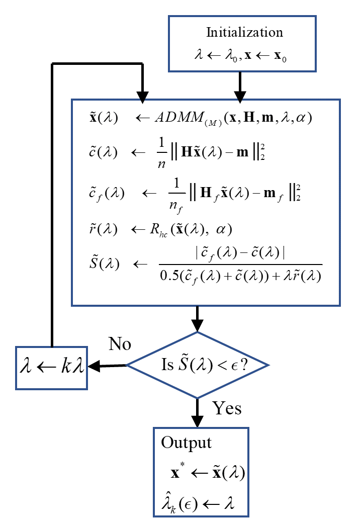
Let be the lowest value of that satisfy . In other words, let . Since is monotonic, this is the same as the condition . Now, since solving this exactly is impractical, we use the following strategy: we define monotonically increasing sequence such that , and find a index such that and . We then declare as an approximation for . We define the sequence in the form where is the real number of the form with being a small positive number. Here, since determines how well approximates , we denotes this approximation by . Determining this way and obtaining the corresponding reconstruction can be represented by the schematic given in Figure 1. In summary, the algorithm of Figure 1 performs reconstruction without the user having to specify the regularization weight directly, and it jointly determines the required regularization weight from the user-specified relative smoothness . One apparent problem in the algorithm is that it brings two additional parameters, viz., and . However, as we will demonstrate in the experiments section, these parameters can be set at a nominal value independent of the measurement vector . In the schematic of Figure 1, we have given computationally efficient formula for by exploiting the fact that the terms and differ only by the data fitting term. We also used the fact that will be zero at . We denote the overall operation of the reconstruction and tracking given in Figure 1 by . Note that, here, denote the initial candidate for reconstruction and is the starting value for used for tacking .

The above scheme only represents an intermediate stage towards developing more pratical method, which is our next goal. The main drawback in the above scheme is that the tracking uses full minimization of the cost for each candidate value of . In the remainder of this section, we develop a more efficient approach that integrates the task of determining an approximation for from a given and the task of obtaining the reconstruction. To this end, we introduce an approximation for , denoted by , as given below:
| (34) |
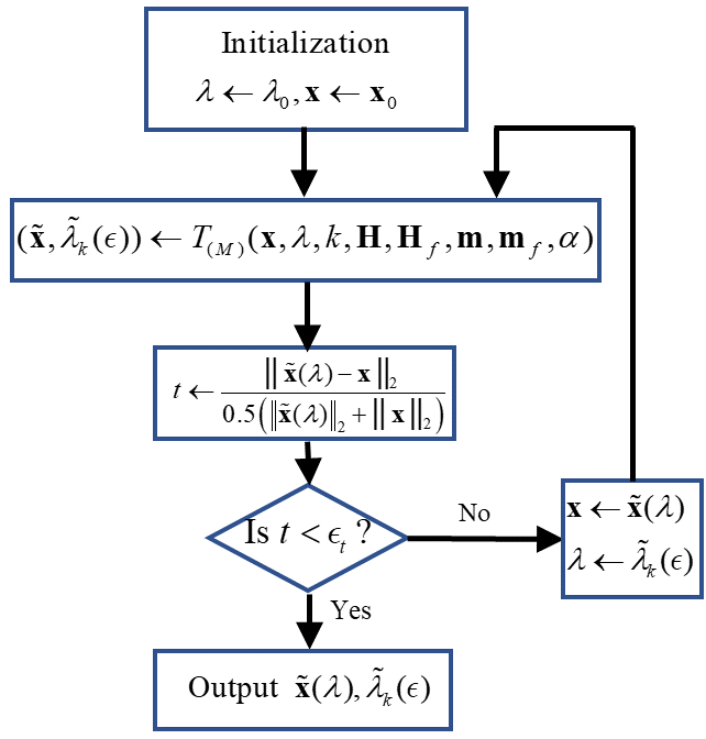
where denotes a partial reconstruction obtained by performing a few ADMM iterations, and and denote the costs obtained from and by removing . The main assumption that will lead the proposed algorithm is that will have a similar type of behaviour provided that the number of ADMM iterations is sufficiently large. Based on this assumption, we propose a modification to the scheme of Figure 1, by merging the minimization of with tracking for . As first step, we define the modified tracking denoted by that is obtained by replacing the minimization by cycles of ADMM iterations, denoted by . Here in denotes the starting point of the iterations. This scheme is given in Figure 2. Note that this approximate scheme brings another parameter, , the number of ADMM iterations performed before each computation of . Again, as we will demonstrate, this can also be fixed at a nominal value independent of the measurement vector .
The final proposed algorithm is the repeated application of this tracking with reconstruction, , where the pair returned by each tracking becomes the initialisation to the next tracking. This process is repeated until relative change in the reconstructed image is lower than the user-defined tolerance . This is given in Figure 3. Comparing with the original tracking scheme of Figure 1, there is no guarantee that this approximate scheme will produce the same results. However, as we demonstrate in the experiment section, the result produced by the approximate scheme has a quality that is comparable to that of the reconstruction obtained by oracle tuning. Note that the final parameter, , is the termination tolerance. As any iterative optimization based image reconstruction, this parameter is set to small positive real number.
4 Experimental results

Four numerical phantoms viz. BloodVessel, Derenzo, PAT, and RatBrain, given in Figure 4 were used to evaluate PAT reconstruction methods. The first three are synthetic phantoms, whereas the last was derived from the MRI angiogram of rat brain published by Pastor et al [pastor2017general]. All were normalized to the size 128 × 128 with a corresponding physical size of 12.8 mm × 12.8 mm as models for generating the synthetic data. The measurement data was generated using a numerical approximation of forward model described in [68] and added with Gaussian noise to form simulated data having SNR levels of 15 dB, 20 dB, 25 dB and 30 dB. The number of transducers to mimic the limited data scenario in our experiments was set to 16. The sound speed in the medium was assumed to be 1.5 mm/ s, and we considered the medium to be homogeneous with no dispersion or absorption of sound. We consider three forms of reconstruction methods for comparative evaluation:
- •
AR-TR: Reconstruction using augmented regularization with proposed tracking of , i.e., the method given in Figure 3.
- •
AR-O: Reconstruction using augmented regularization with oracle tuning of
- •
TV2-O: Reconstruction using TV-2 regularization with oracle tuning of
Our primary goal is to demonstrate the power of augmented regularization with the regularization weight determined using the proposed tracking method of Figure 3. This is taken care by the above list in two ways: (i) comparing AR-TR with AR-O will show how well the power of augmented regularization will be accessible in a practical scenario where the regularization weight is determined from the measurement vector using the proposed tracking; it will also quantify the loss incurred by using the approximations involved in the proposed tacking; (ii) comparing AR-TR with TV2-O will demonstrate that augmented regularization will still have its advantage over the best performing regularization in the literature (TV-2) despite the above-mentioned loss.
The bound on the relatives smoothness, , was fixed at uniformly for all measurement sets independent of noise level and independent of test model used for simulating measurements. Further, the other parameter involved in the tracking algorithm were set as follows: , , and . Again these settings were kept fixed for all input data sets. The relative weight was kept fixed at uniformly for all data sets as we did in our original work [53]. Finally, the termination tolerance was set to . The results are presented in Table 1. We observe the following from the tables:
- •
SSIM scores of reconstructions obtained from AR-TR are comparable to that of the reconstructions obtained from AR-O; in most of cases, the difference is in the third decimal point, and in rare cases, the difference is in the second decimal point. This is significant because AR-O uses the model to determine the value for whereas AR-TR does not.
- •
SSIM scores of reconstructions obtained from AR-TR are significantly better than that of TV2-O, although AR-TR does not use the test model for determining the value for as opposed to TV2-O, which uses the model to determine the value for .
By noting the fact that the required values for AR-TR were tracked from a fixed value of , we conclude from the first observation that the proposed method provide a practical solution to the problem of determining the regularization weight for PAT image reconstruction. The second observation imply that the advantage of augmented regularization over the standard TV regularization is accessible via a practical method for tuning . Note that in our previous work where we introduced the augmented regularization, we demonstrated its superiority over the standard TV only by using oracle tuning.
Note that, among the published methods for regularization weight tuning with total variation regularization, the method of Xue et al. [60] is closest competitor for the the proposed method, AR-TR. However, comparison with TV2-O eliminates the need to compare with method of Xue et al. because TV2-O is bound to give reconstruction that is better than that of the method of Xue et al. due to the oracle tuning in TV2-O. Besides, the method of Xue et al. is based on Monte Carlo simulations, and implementing it for PAT reconstruction will be impractical as PAT forward model is more complex than the blurring model considered by Xue et al. In the remainder of this section, we will display images corresponding to two selected cases from Table 1 and Table 2.
| Phtm. | SNR (dB) | AR-TR | TV2-O | AR-O |
|---|---|---|---|---|
| RatBr | 15 | .916 | .791 | .919 |
| 20 | .955 | .877 | .957 | |
| 25 | .977 | .925 | .979 | |
| 30 | .986 | .956 | .988 | |
| BldVes | 15 | .919 | .719 | .928 |
| 20 | .952 | .827 | .964 | |
| 25 | .980 | .881 | .983 | |
| 30 | .993 | .945 | .993 | |
| Derz | 15 | .995 | .959 | .997 |
| 20 | .999 | .977 | .999 | |
| 25 | .999 | .986 | .999 | |
| 30 | .999 | .989 | .999 | |
| PAT | 15 | .985 | .946 | .985 |
| 20 | .990 | .962 | .990 | |
| 25 | .990 | .973 | .992 | |
| 30 | .991 | .978 | .994 |

Figure 5 compares the reconstructed results for the RatBrain phantom with the measurement set corresponding to SNR level of 15 dB. The original image is given in Figure 5.A while Figure 5.B, 5.C and 5.D gives the reconstructed images from AR-TR, TV2-O, and AR-O respectively. Clearly, AR-TR outperforms TV2-O, which is also confirmed by the fact that the SSIM score of AR-TR’s reconstruction is 0.125 higher than that of TV2-O’s reconstruction. Further, AR-TR’s reconstruction has almost the same quality as that of AR-O. This is confirmed by the fact that the SSIM score of AR-O’s reconstruction is only 0.003 higher than that of AR-TR’s reconstruction. Figure 6 shows the scan-line based intensity profile of the reconstructions of Figure 5 . The intensity profiles show that the proposed method, AR-TR, follows the ground truth as good as the oracle tuning method, AR-O, which is also confirmed by the small difference in the SSIM scores.


Next, for another closer view, we select the reconstruction corresponding to measured data with 15 dB SNR obtained using BloodVessel phantom. The images are given in Figure 7. Figure 7.A shows the BloodVessel phantom and Figures 7.B, 7.C and 7.D gives the reconstructions from the AR-TR, TV2-O, and AR-O respectively. Here also, AR-TR is able to produce a reconstruction with a quality that is comparable to the quality of the reconstructions produced by AR-O, which is confirmed by a mere difference of 0.009 in SSIM. Further, AR-TR retains the advantage that augmented regularization has over the TV-2 regularization, which is confirmed by the improvement of 0.2 in SSIM score. Figure 8 shows the scan-line based intensity profile of the reconstructions in Figure 7. Here also, our method closely follows the ground truth as good as the oracle tuning method, which is also confirmed by the small difference in the SSIM scores.

5 Conclusion
Currently, there is no method for determining the required regularization weight from measured data for PAT image reconstruction with sparsity regularization; users of a sparsity method have to determine the weight by trail and error approach where the reconstruction is performed for a series of values for the regularization weight, , with a visual feed back on the quality of the reconstructed image. This is impractical because the appropriate value of vary drastically with variations in the noise level and the structural contents of the underlying image. In this paper, we addressed this problem by introducing a novel relative smoothness parameter as an implicit function of that is defined through a partial reconstruction. We constructed an iterative method that jointly determines, for given value of relative smoothness, the corresponding and the required reconstruction with augmented sparsity regularization. We demonstrated experimentally that we can get good quality reconstructions from this new method by setting the relativeness parameter at a fixed nominal value independent of the noise level and the nature of the underlying image. We showed that the SSIM scores of reconstructions obtain this way were close to the SSIM scores of reconstructions obtained from the scheme where the underlying images themselves were used for determining the correct value for . Further, other parameters involved in the definition of the relative smoothness measured also have been set at fixed values independent of noise level and the underlying image. This means that, in practical point of view, our method solves the problem of determining the regularization weight from measured data.
References
- [1] Wang L V and Yao J 2016 Nature methods 13 627
- [2] Pramanik M, Ku G, Li C and Wang L V 2008 Medical physics 35 2218–2223
- [3] Beard P 2011 Interface focus 1 602–631
- [4] Zhou Y, Yao J and Wang L V 2016 Journal of biomedical optics 21 061007
- [5] Upputuri P K and Pramanik M 2016 Journal of biomedical optics 22 041006
- [6] Li L, Zhu L, Ma C, Lin L, Yao J, Wang L, Maslov K, Zhang R, Chen W, Shi J et al. 2017 Nature biomedical engineering 1 1–11
- [7] Han Y, Ding L, Ben X L D, Razansky D, Prakash J and Ntziachristos V 2017 Optics letters 42 979–982
- [8] Xia J and Wang L V 2013 IEEE Transactions on Biomedical Engineering 61 1380–1389
- [9] Deán-Ben X, Gottschalk S, Mc Larney B, Shoham S and Razansky D 2017 Chemical Society Reviews 46 2158–2198
- [10] van den Berg P J, Daoudi K, Moens H J B and Steenbergen W 2017 Photoacoustics 8 8–14
- [11] Jo J, Tian C, Xu G, Sarazin J, Schiopu E, Gandikota G and Wang X 2018 Photoacoustics 12 82–89
- [12] Manohar S and Dantuma M 2019 Photoacoustics 16 100134
- [13] Toi M, Asao Y, Matsumoto Y, Sekiguchi H, Yoshikawa A, Takada M, Kataoka M, Endo T, Kawaguchi-Sakita N, Kawashima M et al. 2017 Scientific reports 7 1–11
- [14] Schoustra S M, Piras D, Huijink R, Op’t Root T J, Alink L, Kobold W M F, Steenbergen W and Manohar S 2019 Journal of biomedical optics 24 121909
- [15] Finch D and Patch S K 2004 SIAM journal on mathematical analysis 35 1213–1240
- [16] Kunyansky L A 2007 Inverse problems 23 373
- [17] Xu M and Wang L V 2002 IEEE transactions on medical imaging 21 814–822
- [18] Xu M and Wang L V 2005 Physical Review E 71 016706
- [19] Haltmeier M, Schuster T and Scherzer O 2005 Mathematical methods in the applied sciences 28 1919–1937
- [20] Xu Y and Wang L V 2004 Physical review letters 92 033902
- [21] Burgholzer P, Matt G J, Haltmeier M and Paltauf G 2007 Physical Review E 75 046706
- [22] Hristova Y, Kuchment P and Nguyen L 2008 Inverse problems 24 055006
- [23] Treeby B E and Cox B T 2010 Journal of biomedical optics 15 021314
- [24] Rosenthal A, Ntziachristos V and Razansky D 2013 Current Medical Imaging 9 318–336
- [25] Buehler A, Rosenthal A, Jetzfellner T, Dima A, Razansky D and Ntziachristos V 2011 Medical physics 38 1694–1704
- [26] Qin T, Zheng Z, Zhang R, Wang C and Yu W 2019 Physics in Medicine & Biology 64 195004
- [27] Yao L and Jiang H 2011 Biomedical optics express 2 2649–2654
- [28] Sanny D R, Prakash J, Kalva S K, Pramanik M and Yalavarthy P K 2018 Journal of biomedical optics 23 100502
- [29] Rejesh N A, Pullagurla H and Pramanik M 2013 JOSA A 30 1994–2001
- [30] Shaw C B, Prakash J, Pramanik M and Yalavarthy P K 2013 Journal of Biomedical Optics 18 080501
- [31] Huang C, Wang K, Nie L, Wang L V and Anastasio M A 2013 IEEE transactions on medical imaging 32 1097–1110
- [32] Arridge S R, Betcke M M, Cox B T, Lucka F and Treeby B E 2016 Inverse Problems 32 115012
- [33] Boink Y E, Lagerwerf M J, Steenbergen W, van Gils S A, Manohar S and Brune C 2018 Physics in Medicine & Biology 63 045018
- [34] Frikel J and Haltmeier M 2018 Inverse Problems 34 024006
- [35] Sandbichler M, Krahmer F, Berer T, Burgholzer P and Haltmeier M 2015 SIAM Journal on Applied Mathematics 75 2475–2494
- [36] Haltmeier M, Berer T, Moon S and Burgholzer P 2016 Journal of Optics 18 114004
- [37] Haltmeier M, Neumann L and Rabanser S 2015 Inverse Problems 31 065005
- [38] Dean-Ben X L, Buehler A, Ntziachristos V and Razansky D 2012 IEEE transactions on medical imaging 31 1922–1928
- [39] Gutta S, Kalva S K, Pramanik M and Yalavarthy P K 2018 Medical physics 45 3749–3767
- [40] Prakash J, Sanny D, Kalva S K, Pramanik M and Yalavarthy P K 2018 IEEE transactions on medical imaging 38 1935–1947
- [41] Bhatt M, Gutta S and Yalavarthy P K 2016 JOSA A 33 1785–1792
- [42] Provost J and Lesage F 2008 IEEE transactions on medical imaging 28 585–594
- [43] Betcke M M, Cox B T, Huynh N, Zhang E Z, Beard P C and Arridge S R 2017 IEEE Transactions on Computational Imaging 3 710–721
- [44] Guo Z, Li C, Song L and Wang L V 2010 Journal of biomedical optics 15 021311
- [45] Rudin L I, Osher S and Fatemi E 1992 Physica D: nonlinear phenomena 60 259–268
- [46] Arridge S, Beard P, Betcke M, Cox B, Huynh N, Lucka F, Ogunlade O and Zhang E 2016 Physics in Medicine & Biology 61 8908
- [47] Han Y, Tzoumas S, Nunes A, Ntziachristos V and Rosenthal A 2015 Medical physics 42 5444–5452
- [48] Wang K, Su R, Oraevsky A A and Anastasio M A 2012 Physics in Medicine & Biology 57 5399
- [49] Rosenthal A, Jetzfellner T, Razansky D and Ntziachristos V 2012 IEEE transactions on medical imaging 31 1346–1357
- [50] Zhang Y, Wang Y and Zhang C 2012 Ultrasonics 52 1046–1055
- [51] Bredies K, Kunisch K and Pock T 2010 SIAM Journal on Imaging Sciences 3 492–526
- [52] Hammernik K, Pock T and Nuster R 2017 Variational photoacoustic image reconstruction with spatially resolved projection data Photons Plus Ultrasound: Imaging and Sensing 2017 vol 10064 (International Society for Optics and Photonics) p 100643I
- [53] Rejesh N, Kalva S, Pramanik M and Arigovindan M 2020 Journal of Instrumentation 15 P12028
- [54] Prakash J, Raju A S, Shaw C B, Pramanik M and Yalavarthy P K 2014 Biomedical optics express 5 1363–1377
- [55] Prakash J, Mandal S, Razansky D and Ntziachristos V 2019 IEEE Transactions on Biomedical Engineering 66 2604–2616
- [56] Blu T and Luisier F 2007 IEEE Transactions on Image Processing 16 2778–2786
- [57] Xue F, Luisier F and Blu T 2013 IEEE Transactions on Image Processing 22 1954–1968
- [58] Li J, Luisier F and Blu T 2018 IEEE Transactions on Image Processing 27 92–105
- [59] Ramani S, Blu T and Unser M 2008 IEEE Transactions on image processing 17 1540–1554
- [60] Xue F, Yagola A G, Liu J and Meng G 2016 Inverse Problems in Science and Engineering 24 625–646 (Preprint https://doi.org/10.1080/17415977.2015.1054822) URL https://doi.org/10.1080/17415977.2015.1054822
- [61] Wang K, Ermilov S A, Su R, Brecht H P, Oraevsky A A and Anastasio M A 2011 IEEE transactions on medical imaging 30 203–214
- [62] Rosenthal A, Razansky D and Ntziachristos V 2010 IEEE transactions on medical imaging 29 1275–1285
- [63] Tao M, Yang J and He B 2009 TR0918, Department of Mathematics, Nanjing University
- [64] Wang Y, Yang J, Yin W and Zhang Y 2008 SIAM Journal on Imaging Sciences 1 248–272
- [65] Arigovindan M, Fung J C, Elnatan D, Mennella V, Chan Y H M, Pollard M, Branlund E, Sedat J W and Agard D A 2013 Proceedings of the National Academy of Sciences 201315675
- [66] Bertsekas D 1999 Nonlinear Programming (Athena Scientific)
- [67] Beck A 2017 First-Order Methods in Optimization (MOS-SIAM series on Optimization) chap 6, pp 129–177
- [68] Liu H, Wang K, Peng D, Li H, Zhu Y, Zhang S, Liu M and Tian J 2016 IEEE transactions on medical imaging 35 2546–2557