Dimension Reduction Forests: Local Variable Importance using Structured Random Forests

A random forest (RF) is an ensemble of $M$ randomized decision trees. The random forest kernel between two points $\bm{\mathrm{x}}_{0},\bm{\mathrm{x}}_{1}\in\mathbb{R}^{p}$ is

where $\ell_{m}$ is the number of leaf nodes in the $m$th tree and $\{A_{1}^{m},\dots,A_{\ell_{m}}^{m}\}$ contains the $m$th tree’s leaf nodes with each $A_{u}^{m}\subseteq\mathbb{R}^{p}$ (Scornet 2016). This kernel is equivalent to the empirical probability that $\bm{\mathrm{x}}_{0}$ and $\bm{\mathrm{x}}_{1}$ share a leaf node within the random forest. Our goal is to extract a local variable importance measure from this kernel; however, this measure is only meaningful if the kernel reflects the regression function’s local structure. Currently, the random forest kernel does not exhibit such adaptivity, which makes it difficult to extract local variable importance measures.

To be more concrete, consider the following non-linear regression model of a univariate response on a bivariate predictor: We draw $\bm{\mathrm{X}}_{1},\dots,\bm{\mathrm{X}}_{n}$ independently from the uniform distribution on $[-3,3]^{2}$, with response

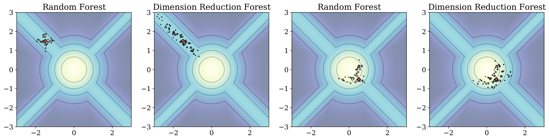
and our goal is to extract local information about the regression (mean) function $m(\bm{\mathrm{x}}_{0})=\mathbb{E}\,[Y\nonscript\;\nonscript\;\bm{\mathrm{X}}=\bm{\mathrm{x}}_{0}]$. Figure 1 displays the contour lines of this function, which depend on three subspaces throughout the function’s domain: $\mathcal{S}_{1}=\spn(\bm{\mathrm{e}}_{1}-\bm{\mathrm{e}}_{2})$ (bottom-left and top-right), $\mathcal{S}_{2}=\spn(\bm{\mathrm{e}}_{1}+\bm{\mathrm{e}}_{2})$ (top-left and bottom-right), and $\mathcal{S}_{3}=\spn(\{\bm{\mathrm{e}}_{1},\bm{\mathrm{e}}_{2}\})$ (center), where $\bm{\mathrm{e}}_{1}$ and $\bm{\mathrm{e}}_{2}$ are the standard basis. An ideal kernel should reflect the local structure by extending its weights along either the orthogonal complement of the one-dimensional subspaces, $\mathcal{S}_{1}$ and $\mathcal{S}_{2}$, or the contour lines within the two-dimensional subspace, $\mathcal{S}_{3}$. The random forest kernel does not exhibit this behavior.

Figure 1 displays the random forest kernel estimated on data from the regression function in Equation (2.2). The RF kernel cannot reflect the local structure because the leaf nodes, $\{A_{u}^{m}\}_{u=1}^{\ell_{m}}$, form an axis-aligned partition of the input space. Indeed, the RF kernel exhibits an axis-aligned plus shape that does not exploit the local dimension reduction structure. As a first encouraging result, our proposed dimension reduction forest’s induced kernel, displayed in Figure 1, warps around the contour lines, improving its performance and accurately reflecting the regression function’s local structure. We develop the dimension reduction forest kernel in Section 3.

Random forests’ popularity is partly due to their ability to produce interpretable global variable importance measures; however, extracting local variable importance is an active research area. As previously mentioned, estimation and inference at the local level are becoming increasingly important, with personalized medicine applications such as inferring individualized therapeutic treatments. Our primary reason for constructing a kernel that can reflect local structure is to uncover such local insights.

As an illustration, we again consider the problem outlined in Equation (2.2); however, now we draw $\bm{\mathrm{X}}_{1},\dots,\bm{\mathrm{X}}_{n}$ independently from a $U[-3,3]^{5}$ so that there are three additional uninformative covariates. Random forests’ global importance measure can indicate that $X_{1}$ and $X_{2}$ are informative; however, it cannot reveal the feature’s heterogeneous contributions throughout the input space.

Figure 2 displays a standard random forest’s global permutation variable importance and our proposed local variable importance measure extracted from a dimension reduction forest at two query points. For regression, the importance assigned by a random forest to a feature is the decrease in mean squared error when the values of that feature are randomly permuted in the out-of-bag samples (Ishwaran and Lu 2018). In contrast, DRF’s local variable importance can be found in Algorithm 2 of Section 3. The random forest only identifies the two significant predictors, while the dimension reduction forest determines the variables’ heterogeneous contribution. At $\bm{\mathrm{x}}_{0}=(-1.5,1.5,0,0,0)^{\rm T}$, the dimension reduction forest correctly indicates that simultaneously increasing or decreasing both $X_{1}$ and $X_{2}$ influences changes in the regression function. In contrast, at $\bm{\mathrm{x}}_{0}=(0.5,-0.5,0,0,0)^{\rm T}$, the DRF indicates that simultaneously increasing $X_{1}$ while decreasing $X_{2}$, or vice versa, is influential. Unlike the random forest’s global importance, the DRF’s local importance results in two drastically different interventions.

Dimension reduction forests are random forests composed of dimension reduction trees that use sufficient dimension reduction (SDR) techniques (Li 1991; Li 2018) to approximate a locally adaptive kernel. Dimension reduction trees are built using a modified classification and regression tree (CART) algorithm (Breiman et al. 1984) with linear combination splitting rules. Specifically, a regression tree $T(\bm{\mathrm{x}}_{0})=\sum_{u=1}^{\ell}\mu_{u}{\mathbbm{1}}\{\bm{\mathrm{x}}_{0}\in A_{u}\}$, with $\ell$ leaf nodes $A_{u}\subseteq\mathbb{R}^{p}$ and leaf means $\mu_{u}\in\mathbb{R}$, is recursively built using a training data set $\mathcal{D}_{n}=\{(Y_{1},\bm{\mathrm{X}}_{i}),\dots,(Y_{n},\bm{\mathrm{X}}_{n})\}$ as follows. At any current leaf node $A$, we search for a splitting rule ${\mathbbm{1}}\{\beta^{\rm T}_{j}\bm{\mathrm{x}}\leq c\}$ for $\beta_{j}\in\mathbb{R}^{p}$ and $j\in\{1,\dots,d\}$, for some $d\leq p$. We set the possible values of the threshold $c$ to all unique values of $\beta_{j}^{\rm T}\bm{\mathrm{X}}_{i}$ within node $A$. We then refine the current leaf node into two child nodes: $A_{L}=A\cap\{\beta^{\rm T}_{j}\bm{\mathrm{x}}\leq c\}$ and $A_{R}=A\cap\{\beta^{\rm T}_{j}\bm{\mathrm{x}}>c\}$ with a certain splitting criterion. In the regression context, the best split minimizes the sum of squared errors in each child node:

where $\mathcal{C}$ is the set of all partitions formed by adding a rule of the form ${\mathbbm{1}}\{\beta^{\rm T}_{j}\bm{\mathrm{x}}\leq c\}$, and $\bar{Y}_{A_{L}}$ and $\bar{Y}_{A_{R}}$ are the mean value of $Y$ inside $A_{L}$ and $A_{R}$, respectively. When we restrict the directions to the standard basis vectors, $\beta_{j}=\mathbf{e}_{j}$ for $j\in\{1,\dots,p\}$, the algorithm reduces to the axis-aligned splits used in the original CART algorithm. Algorithm 1 outlines the procedure for building a dimension reduction forest.

What differentiates DRFs from other random forest variants are splitting directions, $\beta$, estimated through inverse regression, a type of sufficient dimension reduction. Briefly, sufficient dimension reduction aims to find a matrix $B\in\mathbb{R}^{p\times d}$, where $d\leq p$, such that the conditional distribution of $Y$ given $\bm{\mathrm{X}}$ is the same as $Y$ given $B^{\rm T}\bm{\mathrm{X}}$. In regression, this implies that

for an unspecified link function $g(\cdot)$ and random noise $\varepsilon$. This model is equivalent to assuming $Y\perp\bm{\mathrm{X}}\mid B^{\rm T}\bm{\mathrm{X}}$. The column space of $B$, denoted by $\spn(B)$, is called a dimension reduction (DR) subspace. The intersection of all DR subspaces, assuming itself is also a DR subspace, is called the central subspace and denoted by $S_{Y\mid\bm{\mathrm{X}}}$.

Since sufficient dimension reduction does not constrain the form of $g(\cdot)$, it is a powerful tool for designing flexible linear combination splitting rules. This flexibility differentiates our approach from existing oblique forests (Menze et al. 2011; Rainforth and Wood 2015), which impose restrictive linear constraints on the regression surface. Note that DRTs do not necessarily impose any global dimension reduction, such as in Equation (3.2). They only assume meaningful local dimension reduction structures develop as one progressively focuses on more local regions throughout the tree building process, i.e., $Y\perp\bm{\mathrm{X}}\mid B_{A}^{\rm T}\bm{\mathrm{X}}$ for $\bm{\mathrm{X}}\in A\subseteq\mathbb{R}^{p}$ where $B_{A}\in\mathbb{R}^{p\times d}$. Furthermore, we posit that using DRTs within the RF kernel improves its local statistical efficiency by aligning the kernel’s weights with the local Hessian. We elaborate on this point in the next section.

To estimate the sufficient dimension reduction directions, $\{\beta_{1},\dots,\beta_{d}\}$, we use SIR (Li 1991) and SAVE (Cook and Weisberg 1991) since the former is efficient for small sample sizes and the latter is exhaustive. Both methods solve a generalized eigenvalue problem to estimate $B$, which we briefly overview in Section S.1 of the Supplementary Materials. Note that DRTs select the leading eigenvector instead of searching over the full DR subspace. Such an exhaustive search would be redundant because the eigenvalues associated with each direction already measure their local importance. Furthermore, to avoid choosing between SIR and SAVE, we search over the leading directions estimated by both methods when determining a split. This results in a splitting rule that combines the advantages of both SIR and SAVE and performs better than just applying a single method in each node. At the same time, we show that a DRF’s computational complexity remains comparable to traditional random forests in Section S.2 of the Supplementary Materials.

Three problems arise when using traditional SDR methods within dimension reduction forests. First, SIR (SAVE) require at least $p$ samples for inference; however, it is often advisable to set $n_{min}<p$. To accommodate this setting, the DRT searches over axis-aligned splits when the internal node’s sample size is less than $p$. Although this may affect the forest’s ability to adapt to local dimension reduction structures, we found the degradation negligible in practice. Second, the use of dense linear combination splits limits DRF’s applicability in medium to high-dimensional settings. For this reason, we introduce an optional variable screening step in Algorithm 1 that selects covariates based on the minimization of Equation (3.1). Finally, both SIR and SAVE require strong assumptions on the covariates’ joint distribution for consistent estimation. In Section 4, we demonstrate that these assumptions only need to hold at the tree’s root node, extending our method’s applicability to any setting valid for SIR or SAVE.

A recent research initiative aims to improve random forest’s performance by accounting for inefficiencies in the induced random forest kernel function when the regression function has specific properties. For example, local linear forests (Friedberg et al. in press) modify the RF kernel to better model smooth signals through a local linear correction. Here, we argue that dimension reduction forests modify the RF kernel to better model signals with local dimension reduction structure by aligning the induced kernel with the local Hessian. The following argument is heuristic and only serves an illustrative purpose; however, the empirical studies in Section 5 support the conclusions.

We begin by reviewing the bias-variance trade-off in multivariate kernel regression. Consider the multivariate kernel $K(\bm{\mathrm{X}}_{i},\bm{\mathrm{x}}_{0})=\phi\left(\sqrt{(\bm{\mathrm{X}}_{i}-\bm{\mathrm{x}}_{0})^{\rm T}H_{\bm{\mathrm{x}}_{0}}(\bm{\mathrm{X}}_{i}-\bm{\mathrm{x}}_{0})}\right)$, where $\phi(\cdot)$ is a univariate kernel, such as the standard normal density, and $H_{\bm{\mathrm{x}}_{0}}$ is a positive definite $p\times p$ bandwidth matrix that depends on the prediction point $\bm{\mathrm{x}}_{0}$. Under certain regularity conditions, Ruppert and Wand 1994 showed that the bias and variance of the Nadaraya-Watson estimator, $\hat{m}(\bm{\mathrm{x}}_{0})=(\sum_{i=1}^{n}K(\bm{\mathrm{X}}_{i},\bm{\mathrm{x}}_{0}))^{-1}\sum_{i=1}^{n}K(\bm{\mathrm{X}}_{i},\bm{\mathrm{x}}_{0})\,Y_{i}$, conditioned on $\bm{\mathrm{X}}_{1},\dots,\bm{\mathrm{X}}_{n}$ are

where $\mu_{2}(\phi)=\int u^{2}\phi(u)du$, $\lVert\phi\rVert_{2}^{2}=\int\phi(u)^{2}du$, $\sigma^{2}(\bm{\mathrm{x}}_{0})=\operatorname{Var}(Y\nonscript\;\nonscript\;\bm{\mathrm{X}}=\bm{\mathrm{x}}_{0})$, and the density of the covariates is $f_{\bm{\mathrm{X}}}(\cdot)$. Also, $m^{\prime}(\bm{\mathrm{x}}_{0})$ and $m^{\prime\prime}(\bm{\mathrm{x}}_{0})$ indicate the gradient and Hessian of $m(\cdot)$ evaluated at $\bm{\mathrm{x}}_{0}$, respectively. The bias’s first term, also known as the design bias, is often eliminated by applying a local linear correction (Fan and Gijbels 1996). This correction was accounted for in random forests by Friedberg et al. in press. For this reason, we focus on minimizing the second term involving the product of $H_{\bm{\mathrm{x}}_{0}}$ and $m^{\prime\prime}(\bm{\mathrm{x}}_{0})$ while also controlling the variance.

In the presence of local dimension reduction structure, $m(\bm{\mathrm{x}}_{0})=m(B_{\bm{\mathrm{x}}_{0}}^{\rm T}\bm{\mathrm{x}}_{0})$ for some $B_{\bm{\mathrm{x}}_{0}}\in\mathbb{R}^{p\times d}$, where $d<p$. In this case,

where $\bm{\mathrm{u}}_{0}=B_{\bm{\mathrm{x}}_{0}}^{\rm T}\bm{\mathrm{x}}_{0}$ and the Hessian in the third expression is taken with respect to $\bm{\mathrm{u}}_{0}$. This observation implies that $\rank(m^{\prime\prime}(\bm{\mathrm{x}}_{0}))=d_{0}\leq d$, where we assume $d_{0}\neq 0$ for simplicity. According to the bias-variance decomposition given above, one can decrease a kernel estimator’s variance without incurring any additional bias by increasing the bandwidth along the $(p-d_{0})$-dimensional orthogonal compliment of $\spn(m^{\prime\prime}(\bm{\mathrm{x}}_{0}))$, which we denote by $\spn(m^{\prime\prime}(\bm{\mathrm{x}}_{0}))^{\perp}$. Indeed, this can be accomplished by choosing a specific eigendecomposition of $H_{\bm{\mathrm{x}}_{0}}=U_{\bm{\mathrm{x}}_{0}}\Lambda_{\bm{\mathrm{x}}_{0}}U_{\bm{\mathrm{x}}_{0}}^{\rm T}$, where $U_{\bm{\mathrm{x}}_{0}}^{\rm T}U_{\bm{\mathrm{x}}_{0}}=I_{p}$ and $\Lambda_{\bm{\mathrm{x}}_{0}}=\diag(\lambda_{\bm{\mathrm{x}}_{0},1},\dots,\lambda_{\bm{\mathrm{x}}_{0},p})$. Ignoring the design bias, if one selects $\spn(U_{\bm{\mathrm{x}}_{0}})=\spn(m^{\prime\prime}(\bm{\mathrm{x}}_{0}))$, the bias and variance of the estimator in the new basis are

where $\propto$ denotes proportionality between two values, $\Gamma_{d_{0}\times d_{0}}$ is a diagonal matrix of the non-zero eigenvalues of $m^{\prime\prime}(\bm{\mathrm{x}}_{0})$ and $\Lambda_{\bm{\mathrm{x}}_{0}}^{(1)}\in\mathbb{R}^{d_{0}\times d_{0}}$ and $\Lambda_{\bm{\mathrm{x}}_{0}}^{(2)}\in\mathbb{R}^{(p-d_{0})\times(p-d_{0})}$ are also diagonal matrices. The previous two expressions demonstrate that increasing $\Lambda_{\bm{\mathrm{x}}_{0}}^{(2)}$, the bandwidth along $\spn(m^{\prime\prime}(\bm{\mathrm{x}}_{0}))^{\perp}$, reduces the variance without altering the asymptotic bias.

Of course, estimating the appropriate rotation matrix, $U_{\bm{\mathrm{x}}_{0}}$, and bandwidth matrix, $\Lambda_{\bm{\mathrm{x}}_{0}}$, for each sample point $\bm{\mathrm{x}}_{0}$ is computationally infeasible. However, the dimension reduction forest kernel approximates this procedure by recursively using the leading SDR direction to estimate an appropriate rotation and the splitting criterion in Equation (3.1) to estimate an optimal bandwidth along this direction. We use SDR to estimate the splitting direction because the span of the local Hessian lies in the central subspace regardless of the form of $m(\cdot)$. Indeed, $\spn(m^{\prime\prime}(\bm{\mathrm{x}}_{0}))\subseteq\spn(B_{\bm{\mathrm{x}}_{0}})\subseteq S_{Y\mid\bm{\mathrm{X}}}$ by definition.

We propose a heuristic approach to extracting local variable importance from DRFs. Figure 1 demonstrates that the DRF kernel concentrates its bandwidth around the regression function’s contour lines. The previous section gives intuition for this phenomenon, where we argued that the DRF kernel potentially adapts to the subspace spanned by the local Hessian. Note that when the local gradient is non-zero, we also expect this subspace to align with the gradient because $\spn(m^{\prime}(B_{\bm{\mathrm{x}}_{0}}^{\rm T}\bm{\mathrm{x}}))=\spn(B_{\bm{\mathrm{x}}_{0}}m^{\prime}(\bm{\mathrm{u}}))\subseteq\spn(B_{\bm{\mathrm{x}}_{0}})$. In general, given an estimated kernel function, $K_{\text{DRF}}(\bm{\mathrm{x}}_{0},\cdot)$, the subspace of minimum variance about the query point $\bm{\mathrm{x}}_{0}$ potentially aligns with the leading eigenvector of $B_{\bm{\mathrm{x}}_{0}}$ where $\spn(B_{\bm{\mathrm{x}}_{0}})$ is a local DR subspace. Formally, we define this direction as the local subspace variable importance (LSVI) at $\bm{\mathrm{x}}_{0}$. We estimate the LSVI at $\bm{\mathrm{x}}_{0}$ using the smallest principal component of the covariates’ covariance matrix after centering the covariates around $\bm{\mathrm{x}}_{0}$ and weighting them by the dimension reduction forest kernel. We present the full algorithm for estimating LSVIs in Algorithm 2. Only the span of each LSVI is identifiable, which we interpret as the one-dimensional subspace that most influences $m(\bm{\mathrm{x}}_{0})$.

We compared DRFs with two major competitors: traditional random forests as implemented in the scikit-learn Python package and Nadaraya-Watson kernel estimators (NW Kernel). We also included two variations on the traditional random forest (SIR + RF and SAVE + RF) and the Nadaraya-Watson kernel estimator (SIR + NW Kernel and SAVE + NW Kernel). As their names suggest, these two variants first extract global SDR predictors using SIR or SAVE, and then train a random forest or an Nadaraya-Watson kernel estimator using only these features. This approach of using global SDR predictors within a kernel estimator is common practice, see Adragni and Cook 2009. We included these methods to demonstrate the benefit of the recursive dimension reduction performed by DRFs.

We evaluated predictive performance using 50 repeated train-test splits on seven known regression functions. Each split contained $n_{train}=2000$ training samples and $n_{test}=1000$ testing samples. We recorded each method’s mean squared error (MSE) on the test set. The simulations were repeated 50 times with different random seeds. Since machine learning methods are sensitive to hyperparameter settings, it is crucial to explore a large space of values. Table S.1 in the Supplementary Materials lists all hyperparameter settings used in our experiments. To compare each method fairly, we reported the lowest test error achieved by each method over all parameter settings. This procedure differs from the standard practice of using cross-validation to choose the hyperparameters before evaluating on an independent test set. Our approach mitigates the impact of parameter tuning by reporting each method’s best performance over all parameter settings.

For the predictive task, we considered the following four regression functions:

• •

  Simulation 1: $Y=20\max\left\{e^{-2(X_{1}-X_{2})^{2}},\ 2e^{-0.5(X_{1}^{2}+X_{2}^{2})},\ e^{-(X_{1}+X_{2})^{2}}\right\}+\varepsilon$, where $\bm{\mathrm{X}}_{i}\overset{\text{iid}}{\sim}U[-3,3]^{5}$ and $\varepsilon_{i}\overset{\text{iid}}{\sim}N(0,1)$. We presented this regression function in the motivation.

• •

  Simulation 2: $Y=20\max\left\{e^{-18X_{1}^{2}},\ e^{-18X_{2}^{2}},\ 1.75e^{-20(X_{1}+X_{2})^{2}},\ 1.75e^{-20(X_{1}-X_{2})^{2}}\right\}+\varepsilon$, where $\bm{\mathrm{X}}_{i}\overset{\text{iid}}{\sim}U[-1,1]^{5}$ and $\varepsilon_{i}\overset{\text{iid}}{\sim}N(0,1)$.

• •

  Simulation 3: $Y=(\bm{\mathrm{X}}^{\rm T}\beta_{1})^{2}+(\bm{\mathrm{X}}^{\rm T}\beta_{2})^{2}+0.5\varepsilon$. Let $\mathbf{0}_{n}$ denotes an $n$-dimensional vector of zeros. We generate $\bm{\mathrm{X}}_{i}\overset{\text{iid}}{\sim}N(\mathbf{0}_{12},\Sigma)$ and set $\Sigma_{ij}=0.5^{\lvert i-j\rvert}$ resulting in moderate correlation between the covariates. The coefficients are $\beta_{1}=(1,1,1,1,1,1,\mathbf{0}_{6}^{\rm T})^{\rm T}/\sqrt{6}$ and $\beta_{2}=(1,-1,1,-1,1,-1,\mathbf{0}_{6}^{\rm T})^{T}/\sqrt{6}$. Lastly, $\varepsilon_{i}\overset{\text{iid}}{\sim}N(0,1)$.

• •

  Simulation 4: $Y=\bm{\mathrm{X}}^{\rm T}\beta_{1}(\bm{\mathrm{X}}^{\rm T}\beta_{2})^{2}+(\bm{\mathrm{X}}^{\rm T}\beta_{3})(\bm{\mathrm{X}}^{\rm T}\beta_{4})+0.5\varepsilon$, where $\bm{\mathrm{X}}_{i}\overset{\text{iid}}{\sim}N(\mathbf{0}_{10},\Sigma)$, $\Sigma_{ij}=0.5^{\lvert i-j\rvert}$, $\beta_{1}=(1,2,3,4,\mathbf{0}_{6}^{\rm T})^{\rm T}/\sqrt{30}$, $\beta_{2}=(-2,1,-4,3,1,2,\mathbf{0}_{4}^{\rm T})^{T}$ $/\sqrt{35}$, $\beta_{3}=(\mathbf{0}_{4}^{\rm T},2,-1,2,1,2,1)^{T}/\sqrt{15}$, and $\beta_{4}=(\mathbf{0}_{6}^{\rm T},-1,-1,1,1)^{\rm T}/2$. Lastly, $\varepsilon_{i}\overset{\text{iid}}{\sim}N(0,1)$.

We also include the three Friedman functions first introduced in Friedman 1991. We provide the Friedman functions’ definitions in Section S.4 of the Supplementary Materials.

We designed the first two simulations to test the DRF’s ability to adapt to local dimension reduction structure. Simulation 1 is the motivating example in Section 2. Simulation 2 contains four different local one-dimensional subspaces; two are axis-aligned, and two lie in a rotated coordinate system. The next two simulations are commonly used to test SDR methods. We included these regression functions to compare the DRF with a standard random forest trained on SIR and SAVE input features. Finally, Friedman 1–3 are classic regression problems used to test the performance of random forest methods. Here, our goal is to compare DRFs with RFs on problems where DRFs have no clear advantage.

Table 1 displays each method’s mean percentage (100%) improvement over the RF baseline and the corresponding standard deviations for the seven simulation scenarios. The best performing method for each scenario is shaded in gray. A negative value indicates degraded performance, a value of zero indicates no improvement, and a positive value indicates an improvement. Overall, the proposed DRF model performs well in all simulations.

DRFs see some of their largest gains over the competitors in Simulation 1 and Simulation 2. We expected this behavior because these regression surfaces exhibit heterogeneity in the dependent local subspace. Our intuition is that the DRF’s recursive estimation of the local subspace allows it to modify its splitting direction based on the prediction point. The fact that the SIR + RF and SAVE + RF baselines, which can only split along the global DR subspace, have a much higher MSE lends credibility to this assertion.

Simulation 3 and Simulation 4 demonstrate that the DRF’s performance does not degrade when a global SDR subspace adequately describes the regression surface. In Simulation 3, the DRF performs similarly to the SAVE + RF method due to the presence of a global quadratic response surface. However, the DRF drastically outperforms all methods on Simulation 4, which contains a regression surface that is troublesome for SIR and on which SAVE sees only a modest improvement. We conclude that the DRF is a flexible alternative to trying different SDR methods as inputs to nonparametric regressors.

The last three simulations (Friedman 1–3) show that the DRF performs well even when there is no dimension reduction beyond sparsity. In this case, the DRF performs the best or equivalent to the RF baseline. These results demonstrate that the DRF is a reasonable drop-in replacement for the traditional random forest.

Next, we evaluated how the LSVI estimates’ (Algorithm 2) accuracy scaled with (1) a decreasing signal-to-noise ratio and (2) an increase in the number of uninformative covariates. We considered the following four regression functions. Simulation 1: $Y=\lvert X_{1}\rvert+\lvert X_{2}\rvert+\varepsilon$, Simulation 2: $Y=X_{1}+X_{2}^{2}+\varepsilon$, Simulation 3: $Y=5\max\left\{e^{-0.25X_{1}^{2}},e^{-0.25X_{2}^{2}}\right\}+\varepsilon$, and Simulation 4: $Y=20\max\left\{e^{-2(X_{1}-X_{2})^{2}},\ 2e^{-0.5(X_{1}^{2}+X_{2}^{2})},\ e^{-(X_{1}+X_{2})^{2}}\right\}+\varepsilon$. For each simulation, we drew $\bm{\mathrm{X}}_{i}\overset{\text{iid}}{\sim}U[-3,3]^{p}$ and $\varepsilon_{i}\overset{\text{iid}}{\sim}N(0,\sigma^{2})$.

We chose these functions because they exhibit a variety of local dimension reduction structures. Simulation 1 contains the simplest structure with only four local directions that vary by quadrant in the $X_{1}$-$X_{2}$ plane. Simulation 2 contains a simple analytic gradient, $(1,X_{2})^{\rm T}$, that varies along a single direction. This simulation tested whether the LSVI estimates capture smoothly varying local structures. Simulation 3 is composed of a cross of simple one-dimensional axis-aligned subspaces. Simulation 4 is the function in the motivating example, which includes a highly variable local structure.

To evaluate the LSVI estimates’ accuracy, we generated $n=2000$ samples from each regression function and selected $n_{test}=100$ points uniformly at random to test the LSVIs. We recorded the trace correlation between the estimated LSVIs and the normalized gradients at the randomly chosen test points. We repeated each simulation 50 times with different random seeds. To evaluate the effect of a degrading signal-to-noise ratio, we performed the experiments with $p=10$ covariates and set $\sigma^{2}$ so that the signal-to-noise ratio was 5:1, 3:1, 3:2, 1:1, and 3:4. We define the signal-to-noise ratio as $\operatorname{Var}(\mathbb{E}\,[Y\nonscript\;\nonscript\;\bm{\mathrm{X}}])\,/\,\sigma^{2}$.

We compared the LSVIs generated by the following four methods: DRF, SAVE, SIR, and Local SIR. LSVI estimation is sensitive to the DRF’s minimum leaf node size. We searched over $n_{min}\in\{3,10,25,50,100\}$ at each prediction point and reported the best direction in terms of trace correlation to mitigate this effect. Furthermore, we set $m_{try}=5$ for all simulations. The SIR (SAVE) procedure always selects the first principal SDR direction estimated with the standard SIR (SAVE) algorithm with 10 slices. We included these benchmarks to ensure that local structure informs the LSVI algorithm. Local SIR is related to the KNN-SIR method proposed in Wang 2009. For each prediction point, we selected $k\in\{\max(10,p),25,50,100\}$ of the prediction point’s nearest neighbors and estimated the leading SIR direction restricted to these neighbors. We recorded the best trace correlation obtained by the four directions, which correspond to each value of $k$.

Figure 3 displays boxplots of the trace correlations achieved by the four methods at $p=10$ while the signal-to-noise ratio varied. For most scenarios, the DRF procedure performs best with slowly degrading performance as the signal-to-noise ratio decreases. In particular, as the signal-to-noise ratio decrease, the DRF based estimates degenerate to the performance of SAVE. This behavior is especially evident in Scenario 2, where the principal SAVE direction is highly informative. In conclusion, LSVIs produced by DRFs adequately describe the local dimension reduction structure, especially when the signal-to-noise ratio is greater than one.

We include the analysis of how LSVI estimation performed as the number of uninformative covariates increased in Section S.5 of the Supplementary Materials. Our analysis indicated that LSVIs are relatively robust to the number of uninformative covariates, unlike Local SIR, which performed poorly due to the curse of dimensionality.

We applied the dimension reduction forest algorithm to 12 regression data sets taken from the UCI Machine Learning Repository (Dua and Graff 2017) and OpenML (Vanschoren et al. 2013). The 12 data sets represent a variety of regression tasks on real-valued covariates. Table S.2 in the Supplementary Materials displays each data set’s sample size and the number of features. We compared the DRF’s predictive performance to the same six methods included in Section 5.1. For each data set, we performed 15 different rounds of 10-fold cross-validation. We calculated the average out-of-sample MSE over the 10-folds and recorded the percentage (100%) improvement over the random forest baseline. As before, we recorded the best value over the range of hyperparameter settings displayed in Table S.1 of the Supplementary Materials. Table 2 contains the results for the 12 data sets.

Overall, the DRF performs better or equivalent to the RF baseline on most data sets. Specifically, the DRF outperforms the RF on 9 out of 12 data sets. The largest improvements occur either at small sample sizes or where SIR (SAVE) features already result in an improvement. Furthermore, the DRF also saw an improvement in cases where including SIR (SAVE) features hindered the RF’s performance, e.g., on Puma32H and Wisconsin. The only times the DRF method performed worse than the RF is when the SDR features also performed poorly. We conclude that DRFs are a simple alternative to complicated SDR feature engineering with the added benefit that they often improve performance due to their ability to adapt to local structures.

Finally, we demonstrate how to use the LSVIs generated by the DRF algorithm to understand the seasonal variation of PM2.5 (particulate matter) concentration ($\mu g/m^{3}$) in the Chaoyang district of Beijing, China. The raw data was collected by the Urban Air project (Urban Computing Team, Microsoft Research) and consists of meteorological and air quality data collected hourly by 437 air quality stations located in 43 Chinese cities. The data was collected over one year, from May 1st, 2014 to April 30th, 2015. We limited the analysis to observations recorded in Beijing’s Chaoyang district because it is the largest and most populous district. For more details on this data set, see Zheng et al. 2015.

The analysis’s goal is to quantify how different meteorological covariates influence the predictions of PM2.5 concentration throughout the year. We included five covariates in the analysis: month, temperature (^∘C), (atmospheric) pressure (hPa), humidity (%), and wind speed (m/s). We coded the month as an integer from 1 to 12, starting with January. Furthermore, we standardized all covariates so that they have mean zero and unit variance. The final processed data set contained $n=25,794$ observations with $p=5$ covariates. For reference, the pairwise scatter plots and marginal histograms of the covariates used in the analysis are displayed in Figure S.2 of the Supplementary Materials.

We fit a dimension reduction forest to this data set with $M=500$ trees and no feature screening. We selected 3 as the minimum leaf node size using an 80%–20% train-test split to search over $n_{min}\in\{3,5,10\}$. Then, we re-fit the DRF to the full data set with $n_{min}=3$. The model’s in-sample $R^{2}$ is 0.92, indicating a good fit to the data.

To discern how the covariates affected the prediction of PM2.5 concentration, we plotted the LSVI loadings’ marginal distributions in Figure 4. Since the LSVI estimates are invariant to sign changes, we forced the temperature loadings’ sign positive. The largest loadings are on month, humidity, and temperature. Air pressure and wind speed play a less significant role. For comparison, we included the global permutation-based importance extracted from a traditional random forest and a DRF in Figure S.3 of the Supplementary Materials. These results corroborate wind speed’s lack of global importance.

To assess how these effects varied by month, we plotted the loadings’ distributions as a function of month in Figure 4. During the summer months (Jun, Jul, Aug, and Sep), the regression function primarily varies along the subspace spanned by two meteorological variables: temperature + humidity. In contrast, the regression function varies along the subspace spanned by temperature + pressure - humidity in the remaining months. This finding indicates that PM2.5 concentration’s cause varies by season (Chen et al. 2020).

References

- Adragni and Cook (2009) Adragni, K. P. and Cook, R. D. (2009), “Sufficient dimension reduction and prediction in regression,” Philosophical Transactions of the Royal Society A: Mathematical, Physical and Engineering Sciences, 367, 4385–4405.
- Amaratunga et al. (2008) Amaratunga, D., Cabrera, J., and Lee, Y.-S. (2008), “Enriched random forests,” Bioinformatics, 24, 2010–2014.
- Athey et al. (2019) Athey, S., Tibshirani, J., and Wager, S. (2019), “Generalized random forests,” The Annals of Statistics, 47, 1148–1178.
- Athey and Wager (2018) Athey, S. and Wager, S. (2018), “Estimation and inference of heterogeneous treatment effects using random forests,” Journal of the American Statistical Association, 113, 1228–1242.
- Biau (2012) Biau, G. (2012), “Analysis of a Random Forests Model,” Journal of Machine Learning Research, 13, 1063–1095.
- Biau and Scornet (2016) Biau, G. and Scornet, E. (2016), “A random forest guided tour,” TEST, 25, 197–227.
- Breiman (2001) Breiman, L. (2001), “Random forests,” Machine Learning, 45, 5–32.
- Breiman et al. (1984) Breiman, L., Freidman, J., Olshen, R., and Stone, C. (1984), Classification and Regression Trees, Pacific Grove, CA: Wadsworth International.
- Chen et al. (2020) Chen, Z., Chen, D., Zhao, C., Kwan, M., Cai, J., Zhuang, Y., Zhao, B., Wang, X., Chen, B., Yang, J., Li, R., He, B., Gao, B., Wang, K., and Xu, B. (2020), “Influence of meteorological conditions on PM2.5 Concentrations across China: A review of methodology and mechanism,” Environmental International, 139, 105558.
- Cook and Weisberg (1991) Cook, R. D. and Weisberg, S. (1991), “Sliced Inverse Regression for Dimension Reduction: Comment,” Journal of the American Statistical Association, 86, 328–332.
- Cui et al. (in press) Cui, Y., Zhu, R., Zhou, M., and Kosorok, M. R. (in press), “Consistency of Survival Tree and Forest Models: Splitting Bias and Correction,” Statistica Sinica, doi:10.5705/ss.202020.0263.
- Diaz-Uríarte and de Andrés (2006) Diaz-Uríarte, R. and de Andrés, S. A. (2006), “Gene Selection and Classification of Microarray Data using Random Forests,” BMC Bioinformatics, 7.
- Dua and Graff (2017) Dua, D. and Graff, C. (2017), “UCI Machine Learning Repository [http://archive.ics.uci.edu/ml],” Irvine, CA: University of California, School of Information and Computer Science.
- Fan and Gijbels (1996) Fan, J. and Gijbels, I. (1996), Local polynomial modelling and its applications, vol. 66 of Monographs on Statistics and Applied Probability, London: Chapman and Hall.
- Friedberg et al. (in press) Friedberg, R., Tibshirani, J., Athey, S., and Wager, S. (in press), “Local Linear Forests,” Journal of Computational and Graphical Statistics, doi:10.1080/10618600.2020.1831930.
- Friedman (1991) Friedman, J. H. (1991), “Multivariate adaptive regression splines,” The Annals of Statistics, 19, 1–67.
- Geurts et al. (2006) Geurts, P., Ernst, D., and Wehenkel, L. (2006), “Extremely randomized trees,” Machine Learning, 63, 3–42.
- Hothorn et al. (2004) Hothorn, T., Lausen, B., Benner, A., and Radespiel-Tröger, M. (2004), “Bagging survival trees,” Statistics in Medicine, 23, 77–91.
- Ishwaran et al. (2008) Ishwaran, H., Kogalur, U. B., Blackstone, E. H., and Lauer, M. S. (2008), “Random Survival Forests,” The Annals of Applied Statistics, 2, 841–860.
- Ishwaran and Lu (2018) Ishwaran, H. and Lu, M. (2018), “Standard errors and confidence intervals for variable importance in random forest regression, classification, and survival,” Statistics in Medicine, 38, 558–582.
- Laber and Zhao (2015) Laber, E. B. and Zhao, Y. Q. (2015), “Tree-based methods for individaulized treatment regimes,” Biometrika, 102, 501–514.
- Li (2018) Li, B. (2018), Sufficient Dimension Reudction: Methods and Applications with R, Monographs in Statistics and Applied Probability, Boca Raton: Chapman and Hall/CRC.
- Li (1991) Li, K.-C. (1991), “Sliced Inverse Regression for Dimension Reduction,” Journal of the American Statistical Association, 86, 316–327.
- Lin et al. (2018) Lin, Q., Zhao, Z., and Liu, J. S. (2018), “On Consistency and Sparsity for Sliced Inverse Regression in High Dimensions,” The Annals of Statistics, 46, 580–610.
- Lin et al. (2019) — (2019), “Sparse Sliced Inverse Regression via Lasso,” Journal of the American Statistical Association, 114, 1726–1739.
- Lin and Jeon (2006) Lin, Y. and Jeon, Y. (2006), “Random Forests and Adaptive Nearest Neighbors,” Journal of the American Statistical Association, 101, 578–590.
- Loyal (2021) Loyal, J. D. (2021), “Package and replication code for “Dimension Reduction Forests: Local Variable Importance using Structured Random Forests",” https://github.com/joshloyal/drforest.
- Ma and Zhu (2012) Ma, Y. and Zhu, L. (2012), “A semiparametric approach to dimension reduction,” Journal of the American Statistical Association, 107, 168–179.
- Meinshausen (2006) Meinshausen, N. (2006), “Quantile Regression Forests,” Journal of Machine Learning Research, 7, 983–999.
- Mentch and Hooker (2016) Mentch, L. and Hooker, G. (2016), “Quantifying uncertainty in random forests via confidence intervals and hypothesis tests,” The Journal of Machine Learning Research, 17, 841–881.
- Menze et al. (2011) Menze, B. H., Kelm, B. M., Splitthoff, D. N., Koethe, U., and Hamprecht, F. A. (2011), “On oblique random forests,” in Joint European Conference on Machine Learning and Knowledge Discovery in Databases, Springer, pp. 453–469.
- Prasad et al. (2006) Prasad, A. M., Iverson, L. R., and Liaw, A. (2006), “Newer Classification and Regression Tree Techniques: Bagging and Random Forests for Ecological Prediction,” Ecosystems, 9, 181–199.
- Rainforth and Wood (2015) Rainforth, T. and Wood, F. (2015), “Canonical Correlation Forests,” arXiv preprint arXiv:1507:05444.
- Ruppert and Wand (1994) Ruppert, D. and Wand, M. P. (1994), “Multivariate Locally Weighted Least Squares Regression,” The Annals of Statistics, 22, 1346–1370.
- Scornet (2016) Scornet, E. (2016), “Random Forests and Kernel Methods,” IEEE Transactions on Information Theory, 62, 1485–1500.
- Strobl et al. (2008) Strobl, C., Boulesteix, A.-L., Kneib, T., Augustin, T., and Zeileis, A. (2008), “Conditional variable importance for random forests,” BNC Bioinformatics, 9.
- Vanschoren et al. (2013) Vanschoren, J., van Rijn, J. N., Bischl, B., and Torgo, L. (2013), “OpenML: networked science in machine learning,” SIGKDD Explorations, 15, 49–60.
- Wang (2009) Wang, Q. (2009), “Sufficient Dimension Reduction and Sufficient Variable Selection,” Ph.D. thesis, The University of Georgia.
- Zheng et al. (2015) Zheng, Y., Yi, X., Li, M., Li, R., Shan, Z., Chang, E., and Li, T. (2015), “Forecasting Fine-Grained Air Quality Based on Big Data,” in Proceedings of the 21th SIGKDD conference on Knowledge Discovery and Data Mining.
- Zhu et al. (2015) Zhu, R., Zeng, D., and Kosorok, M. R. (2015), “Reinforcement Learning Trees,” Journal of the American Statistical Association, 110, 1770–1784.
Supplementary Material for
- Golub and Loan (2012) Golub, G. G. and Loan, C. F. V. (2012), Matrix Computations, vol. 3, Baltimore and London: The Johns Hopkins University Press.
- Louppe (2014) Louppe, G. (2014), “Understanding random forests: From theory to practice,” arXiv preprint arXiv:1407.7502.
- Silverman (1986) Silverman, B. W. (1986), Density Estimation for Statistics and Data Analysis, London: Chapman and Hall/CRC.