Vulnerability of Appearance-based Gaze Estimation
Abstract
Appearance-based gaze estimation has achieved significant improvement by using deep learning. However, many deep learning-based methods suffer from the vulnerability property, i.e., perturbing the raw image using noise confuses the gaze estimation models. Although the perturbed image visually looks similar to the original image, the gaze estimation models output the wrong gaze direction. In this paper, we investigate the vulnerability of appearance-based gaze estimation. To our knowledge, this is the first time that the vulnerability of gaze estimation to be found. We systematically characterized the vulnerability property from multiple aspects, the pixel-based adversarial attack, the patch-based adversarial attack and the defense strategy. Our experimental results demonstrate that the CA-Net shows superior performance against attack among the four popular appearance-based gaze estimation networks, Full-Face, Gaze-Net, CA-Net and RT-GENE. This study draws the attention of researchers in the appearance-based gaze estimation community to defense from adversarial attacks.
1 Introduction

Eye gaze is one of the important channel for communication. It indicates the region of interest during eye typing [17, 24], authentication [13, 19], saliency prediction [31], object detection [7] and so on. Estimating gaze direction from eye appearance is challenging due to the diversity of human eyes. Conventional model-based gaze estimation approach seeks to recover the gaze direction from 3D eye model, but it usually requires dedicated devices such as infrared cameras. In contrast, the appearance-based gaze estimation approach only uses inexpensive web cameras, and directly learns the mapping function from eye/face images to gaze directions [20, 21].
With the development of deep learning, the appearance-based gaze estimation accuracy has been significantly improved. A number of deep learning-based gaze estimation methods have been proposed. Sugano et al. introduced learning-by-synthesis approach [28] to appearance-based gaze estimation. Zhang et al. introduced the appearance-based gaze estimation method [32] based on LeNet [18] using a grayscale single eye image as input. The backbone network of [32] was changed to a 16-layer VGGNet [27] afterwards, which was described in Zhang et al. [34]. Zhang et al. used the full face image from the MPIIFaceGaze dataset to estimate gaze angles [33]. Cheng et al. explored the asymmetric of two eyes and improved the gaze estimation accuracy [5, 6]. Fischer et al. introduced a new dataset which makes ground truth annotation more accurately with eyetracking glasses, uses semantic image inpainting to remove glasses and presents a new real-time algorithm for gaze estimation [8]. Park et al. used very few examples to calibrate the model in order to learn the person-specific gazes [25]. Cheng et al. proposed a coarse-to-fine strategy [4] where the full face is used to obtain coarse-grained gaze direction and the combination of full face and two eyes are used for fine-grained gaze direction. Bao et al. recently proposed an effective method [1] that works well in mobile tablets.
However, the deep learning-based classification task often appears vulnerability [29, 10], i.e., adding invisible noise on to the raw image leads to dramatic changes of network output. This problem can be summarized as following: given an input image that belongs to the target class , we can easily generate the adversarial example similar to to be classified as . Szegedy et al. first discovered the vulnerability of deep learning models [29]. Goodfellow et al. used one-step fast gradient sign method [10] to attack the classification models. Kurakin et al. introduced Basic Iterative Method (BIM) [16], which is an iterative method for attacking. Madry et al. used project gradient descent in the attack task [22]. Carlini et al. introduced attacks that are tailored to , and distance metrics [3]. Brown et al. place a patch on images to make the images misclassified [2], which is different from the attack methods described above.
In this paper, we investigate whether the vulnerability also exist in appearance-based gaze estimation task. By adding adversarial perturbation to the original inputs, we study if it is possible to change the predicted gaze direction, or even output a specific gaze direction. Fig. 1 shows the pipeline of this paper.
The main contributions of this paper are:
- •
To our knowledge, we are the first to show the existence of the vulnerability in the appearance-based gaze-estimation tasks. We use the regression approach instead of classification to investigate the properties of vulnerability.
- •
We conduct a systematic study of vulnerability in terms of three aspects: the pixel-based adversarial attack, the patch-based adversarial attack and the defense strategy. We characterize the vulnerability from multiple aspects: hyper-parameters, face regions, model attention, smoothness, etc.
- •
We report the performance of typical gaze estimation networks being attacked. We also evaluate the defense performance of these networks. Based on these results, we emphasize the necessity of defense in future appearance-based gaze estimation studies.
2 Study overview
2.1 Study architecture
This paper focuses on the vulnerability of appearance-based gaze estimation tasks. We characterize the vulnerability from two aspects, the attack side and the defense side. On the attack side, we investigate using pixel-based noise (Sec. 3) and patch-based noise (Sec. 4) to attack the existing gaze estimation networks. We show the existence of the vulnerability and investigate the mechanism of vulnerability. We evaluate the performance of the attack under different parameter settings (Sec. 3.2.1), and attack the different parts of the face (Sec. 3.2.2) to understand the roles of each face region during gaze estimation. We study the smoothness effect (Sec. 3.2.3) to make the perturbations more invisible. To make the attack physically applicable, we investigate the patch-based adversarial attack and evaluated the performance of it (Sec. 4.2). We also explore how to defend against attacks, which is in Sec. 5.
2.2 Gaze estimation network
To evaluate the vulnerability of appearance-based gaze estimation tasks, we select four typical gaze estimation networks, Full-Face [33], Gaze-Net [34], CA-Net [4] and RT-GENE [8]. We introduce the details of these networks below. (The training data is randomly shuffled for each epoch.)
Full-Face [33]. This method is based on AlexNet [14] and uses the full face images as input. It is one of the most widely used method in appearance-based gaze estimation area. We used the MPIIFaceGaze dataset described in [33]. The batch size is , the base learning rate is and weight_decay is . We used SGD optimizer with momentum=0.9 and nesterov=True and multi-step scheduler with and milestones=(on epochs). The model is for epochs with loss.
Gaze-Net [34]. This method is based on the pretrained VGG-16 [27] and used grayscale single eye images as input. We use this method as it is the first CNN-based method for gaze estimation and often used as the baseline. We used MPIIGaze dataset described in [34]. The batch size is and the base learning rate is . We used Adam optimizer with and and the StepLR scheduler with and . The model is trained for epochs with MSE loss. We used MSRA initialization [11] to linear layers.
CA-Net [4]. CA-Net uses two eyes and the full face as input. Observed from the latter study, CA-Net shows superior performance against attack among the methods we used. This method is chosen as it achieves the state-of-the-art performance on MPIIFaceGaze [33] and EYEDIAP [9] dataset (with Person #12-#13 removed as described in [4]). The batch size is , the base learning rate to and . We used SGD optimizer. The model is trained for epochs. We used MSRA initialization [11] to Conv2d layers.
RT-GENE [8]. This method has more accurate ground truth obtained by eye tracking glasses. We use ResNet-18 [12] backbone model due to the low computation cost. This method used two gray-scale eye images as input. We have trained two models with (described as RT-GENE) and without (described as RT-GENE (Augmented)) data augmentation, respectively. The batch size is and base learning rate is . We trained the model with MSE loss. The model is trained for 5 epochs if data augmentation is disabled or 64.
2.3 Attack task definition
Our goal is to confuse the gaze estimation model and output the certain target gaze direction. Given an appearance-based gaze estimator and the 3D target gaze direction , we generate the adversarial example by minimizing the angular error between the estimated gaze direction and the target direction , as shown below:
| (1) |
where the angular error is defined as:
| (2) |
Note that we have used instead of since we may have multiple inputs fed into the gaze estimator. constrains the distance between and to make similar to .
In this paper, we use the angular error between the estimated gaze direction and the target gaze direction to measure the vulnerability of the gaze estimation networks. The unit of angular error is degree. The smaller is, the more vulnerable the method is, since the network outputs can easily changed. Meanwhile, we also measure angular error between the estimated gaze direction and the ground truth gaze direction. Large means that the estimated gaze direction after attack is far from the ground truth, which also indicates the vulnerability.
Without loss of generality, we denote the 2D target gaze directions as (, ) and select four target gaze directions in the target attack task. As shown in the right part of Fig. 1, we use , , , and to represent four target directions and . Each dataset is divided into several folds according to the person. We follow the leave-one-person-out strategy to train and test the model. For example, we train on the Person #1-#14 of MPIIGaze, then test and attack on Person #0. If no special instruction, we only use one fold of the dataset (Person #0 for MPIIFaceGaze and MPIIGaze, Person #1 for EYEDIAP, Fold #0 for RT-GENE) for each method to attack, and the other folds to train the model. The final result is the mean angle loss across these four target directions and all the inputs inside the corresponding fold.
In practice, a batch of input images instead of one input image will be used for the optimization task. If there are more than one type of output, e.g., the coarse output and the fine output, we use the sum of angular error of each type of output. If there are more than one type of input, e.g., the eyes and the face, each type of input will be attacked independently.
3 Study on pixel-based adversarial attack
3.1 Method
The pixel-based adversarial attack is the modified from the Basic Iterative Method (BIM) [15], which is described as follows:
| (3) |
where is the iteration index, means clipping to the range that meets the constriant. The final adversarial example is the that minimizes .
There are three hyper-parameters, , and , where represents the intensity of the constraint, is the stride of one iteration, and is the number of iterations. The original paper [15] sets and . Here we modified to to guarantee fairness for different and .
3.2 Characterization
3.2.1 Performance analysis
First, we evaluate the effects of model parameters and . The testing range of is , the testing range of is . In theory, the maximum possible value of is 255. Here we choose the maximum value of as 64 since it is large enough to generate the typical attack results. In the original paper [15], the authors set to be 1. Here we test a wider range of from 0.125 to 4 to see the influence of on attack task. The results of mean angular error under different combinations of and can be found in Table 1. The “Heatmaps” in the right column of the table visualize the changing trend.
We observe that the angular error increases as the stride size increases. This may be due to that smaller stride leads the model to be attacked more granularly while the larger stride makes the loss more difficult to converge. For Full-Face, Gaze-Net and RT-GENE, the mean angular error significantly decreases as increases. In other words, the network becomes easier to be attacked. It can be inferred that these models have strong vulnerability. However, the mean angular error of CA-Net decays very slowly when testing on MPIIFaceGaze and EYEDIAP, which indicates that this model is robust. From the heatmaps in Table 1, we also observe that when increases, the mean angular errors of different methods decay at different speeds. This indicates different vulnerability of different methods in terms of : Full-Face RT-GENE RT-GENE (Augmented) Gaze-Net CA-Net. This conclusion suggest that the CA-Net is most robust against the attacks.
| Dataset + Method | Mean angular error when | Heatmap of angular error | |||||||
|---|---|---|---|---|---|---|---|---|---|
| 1 | 2 | 4 | 8 | 16 | 32 | 64 | |||
| MPIIFaceGaze [33] + Full-Face [33] | 4 | 44.97 | 38.52 | 19.16 | 10.05 | 8.933 | 8.932 | 8.868 | |
| 2 | 44.97 | 26.60 | 12.29 | 9.533 | 9.221 | 8.204 | 6.624 | ||
| 1 | 39.01 | 20.08 | 8.603 | 7.337 | 6.158 | 4.918 | 3.759 | ||
| 0.5 | 36.11 | 17.13 | 4.911 | 3.812 | 3.110 | 2.569 | 2.098 | ||
| 0.25 | 35.14 | 13.05 | 2.367 | 1.956 | 1.648 | 1.421 | 1.242 | ||
| 0.125 | 33.79 | 11.24 | 1.295 | 1.048 | 0.852 | 0.674 | 0.551 | ||
| RT-GENE [8] | 4 | 51.37 | 49.04 | 38.22 | 28.29 | 20.34 | 12.39 | 8.001 | |
| 2 | 51.37 | 40.97 | 29.94 | 20.89 | 12.23 | 7.282 | 4.812 | ||
| 1 | 46.67 | 35.50 | 24.44 | 14.05 | 7.907 | 4.812 | 3.207 | ||
| 0.5 | 44.06 | 32.42 | 19.01 | 10.36 | 5.716 | 3.555 | 2.371 | ||
| 0.25 | 42.84 | 29.22 | 16.05 | 8.261 | 4.401 | 2.744 | 1.810 | ||
| 0.125 | 41.66 | 27.74 | 14.56 | 6.977 | 3.522 | 2.100 | 1.326 | ||
| RT-GENE [8] (Augmented) | 4 | 49.73 | 48.88 | 41.59 | 34.33 | 26.42 | 14.71 | 8.527 | |
| 2 | 49.73 | 42.26 | 34.66 | 26.33 | 14.89 | 8.218 | 4.870 | ||
| 1 | 45.02 | 36.82 | 28.43 | 17.00 | 9.006 | 4.905 | 2.846 | ||
| 0.5 | 42.05 | 33.35 | 21.88 | 11.92 | 6.081 | 3.265 | 1.919 | ||
| 0.25 | 40.56 | 29.67 | 18.23 | 9.433 | 4.644 | 2.479 | 1.444 | ||
| 0.125 | 39.11 | 27.74 | 16.29 | 8.101 | 3.861 | 2.047 | 1.235 | ||
| MPIIGaze [34] + Gaze-Net [34] | 4 | 57.62 | 55.55 | 51.38 | 44.08 | 34.24 | 20.37 | 7.570 | |
| 2 | 57.62 | 54.94 | 50.07 | 42.45 | 30.85 | 16.83 | 5.354 | ||
| 1 | 57.47 | 54.65 | 49.67 | 41.21 | 29.01 | 14.75 | 3.982 | ||
| 0.5 | 57.43 | 54.61 | 49.38 | 40.61 | 27.94 | 13.24 | 2.918 | ||
| 0.25 | 57.43 | 54.55 | 49.25 | 40.31 | 27.29 | 12.13 | 2.117 | ||
| 0.125 | 57.42 | 54.53 | 49.21 | 40.18 | 26.93 | 11.39 | 1.617 | ||
| EYEDIAP [9] + CA-Net [4] | 4 | 52.28 | 50.16 | 45.77 | 43.04 | 41.40 | 39.91 | 39.19 | |
| 2 | 52.28 | 47.75 | 44.29 | 41.73 | 39.77 | 38.90 | 38.29 | ||
| 1 | 50.55 | 46.22 | 42.91 | 40.12 | 38.94 | 38.26 | 37.84 | ||
| 0.5 | 49.52 | 45.35 | 41.72 | 39.42 | 38.53 | 38.01 | 37.66 | ||
| 0.25 | 49.06 | 44.48 | 41.18 | 39.25 | 38.43 | 37.93 | 37.60 | ||
| 0.125 | 48.78 | 44.17 | 41.07 | 39.42 | 38.42 | 37.90 | 37.57 | ||
| MPIIFaceGaze [33] + CA-Net [4] | 4 | 53.81 | 51.64 | 45.74 | 42.03 | 40.09 | 38.72 | 38.08 | |
| 2 | 53.81 | 48.56 | 43.82 | 40.76 | 38.79 | 38.00 | 37.57 | ||
| 1 | 51.88 | 47.07 | 42.80 | 39.72 | 38.19 | 37.62 | 37.38 | ||
| 0.5 | 50.99 | 46.39 | 41.93 | 39.38 | 38.01 | 37.51 | 37.29 | ||
| 0.25 | 50.54 | 45.53 | 41.60 | 39.34 | 38.02 | 37.52 | 37.30 | ||
| 0.125 | 50.14 | 45.23 | 41.49 | 39.40 | 38.23 | 37.80 | 37.59 | ||
Figure 2 visualizes the perturbed images under different . Since represents the intensity of constriant, it can be inferred that greater may lead to farther distance between and , and the perturbations may become more obvious. For example, when and (Fig. 2(d), 2(e), 2(f), 2(g), 2(h), 2(i)), the perturbation become more obvious as getting larger. However, in some cases this conclusion is false. For example, when (2(a), 2(b), 2(c)), the perturbation is not obvious even though is high enough.


We also investigate the wide vulnerability of models. While the experiments above are all limited to a single fold of dataset, we also conduct experiments attacking on each folds for every model. As and get the most best results in Table 1, we choose this combination of and . For each model we compute the mean and standard deviation of angular error across all inputs and targets. The results are displayed in Table 2. We observed that the angular error of Full-Face, Gaze-Net and RT-GENE are all close to , indicating that the estimated gaze directions for these models are easily to be changed. This result shows the wide and strong vulnerability of these models.
| Dataset+Method | Mean angular error |
|---|---|
| MPIIFaceGaze[33]+Full-Face[33] | 0.600.48 |
| MPIIGaze[34]+Gaze-Net[34] | 0.641.76 |
| EYEDIAP [9]+ CA-Net[4] | 37.407.14 |
| MPIIFaceGaze [33]+ CA-Net[4] | 36.5210.12 |
| RT-GENE [8] | 1.773.95 |
| RT-GENE [8](Augmented) | 3.215.78 |
However, the angular error of CA-Net is still very high even though becomes very large. We found that the standard deviation of CA-Net is larger than that of other models, so we show the results of CA-Net within each target in Table 3. We also choose and . It can be found that although the standard deviation of CA-Net in 2 is very large, the difference within one target is relatively small, which indicates that towards a certain target, the estimated gaze directions after attack are centered at a value that is far from the target. This result clearly illustrates the robustness of CA-Net.
3.2.2 Face regions effects
While the attacks on Full-Face performed above are only for the full face, it is necessary to know the effect of attacking different face regions. The face regions are shown in Figure 3, including “Eyes”, “Nose”, “Mouth” and “Others” (the rest parts of the face). Here we conduct the attack experiment on Full-Face model and show the results when . This is because these hyper-parameters generate the typical results. Table 4 displays the result. We found that the attack on “Eyes” achieves the lowest angular error. This can be explained that before attack, “Eyes” is the most focused region in Figure 4, which indicates that “Eyes” is the most vulnerable part for attacks. Interestingly, attack on “Others” performs relatively poor although its mean angle error is low enough.

To investigate the reason behind vulnerability and how the attack influences the model, we visualized the attention patterns using Score-CAM [30] on Full-face model, as shown in Figure 4. It can be observed that “Others” does not attract much attention, and Figure 4(d) illustrates that the attention pattern is diluted after the attack. It can be concluded that the attention pattern changes even though we attack on such unimportant part, thus it validates the model vulnerability. We also observe that the system achieves large angular error when we only attack on either “Nose” or “Mouth”. Figure 4(b) and 4(c) shows that the attention area is only “Nose” or “Mouth” after attack. If both “Nose” and “Mouth” are attacked, much lower angular error can be achieved and the attention area also transfers to both “Nose” and “Mouth” after attack. But this angular error is still higher than that performed by attack on some other parts. Note that all the attention areas are not on “Eyes”, which leads to such result. If we attack on both “Eyes” and “Nose”, or both “Eyes” and “Mouth”, the mean angular error becomes much lower compared to the attack on “nose” or “mouth” only. In this case, the attention area is on both “Eyes” and some other parts.
Based on the attention patterns, we found that if the attention of “Eyes” is strong as in Figure 4(a), 4(e), 4(g) and 4(h), the system achieves very low angular error. If the attention of “Eyes” exists but it is not strong, e.g., Figure 4(d) and 4(i), low angular error can also be obtained but higher than the previous case; if the attention of “Eyes” almost does not exist, we can only achieve large angular error as shown in Figure 4(b), 4(c) and 4(f).
| Face parts | Angular error |
|---|---|
| Eyes | 0.2830.374 |
| Nose | 30.3312.53 |
| Mouth | 26.6118.05 |
| Others | 1.0470.651 |
| Nose+Mouth | 4.4027.710 |
| Eyes+Nose | 0.3200.372 |
| Eyes+Mouth | 0.3410.383 |
| Eyes+Nose+Mouth | 0.4120.422 |
| Eyes+Nose+Mouth+Others | 1.4210.614 |
3.2.3 Smoothness
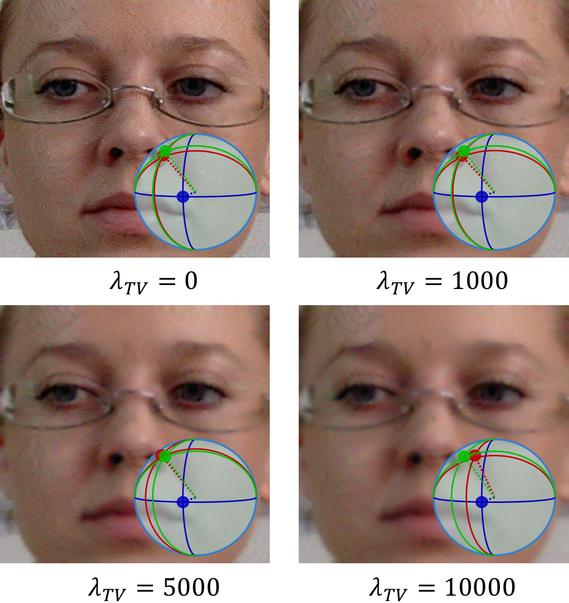
From Fig. 2, We observed that sometimes the adversarial perturbation using large is obvious enough to be distinguished. From the perspective of the attacker, this makes the application of attacks limited. To make the perturbation more smooth, we introduce the total variation loss [23]. Here we modify the objective function (2) to:
| (4) |
where controls the weights between the angular error and the total variation loss, is the total variation loss, defined as:
| (5) |
Figure 5 illustrates the result of smoothness, we observe that when we increase , the perturbed image becomes smoother. However, the attacked gaze direction only slightly changes, this validates the vulnerability of the gaze estimation models, even indistinguishable noise could perturb the network prediction.
4 Study on patch-based adversarial attack
4.1 Method
Although the pixel-based method is effective for attack on appearance-based gaze estimation as discussed in Section 3, it is difficult to make such method physically realizable. Due to this reason, we draw on the idea of adversarial patch [2] and place a patch on the face common to all the input images (including the content and the position of the patch), as shown in Fig. 6, instead of adding adversarial perturbation directly on the face. In order to make the face detectable, we do not place the patch on the landmarks of the face.
First, we define the adversarial example as:
| (6) |
where is element-wise multiplication, is the patch whose size is the same as , means belongs to the patch and means doesn’t belong to the patch. Obviously, defines the region of the patch.
The patch-based method is also based on the idea of Basic Iterative Method (BIM) method [15]:
| (7) |
where is the index of the current iteration. If the current is the first image to input, is the randomly initialized image. Otherwise, is the related to the minimum angular error of the previous image. Note that all the images used to generate the patch will be iterated for epochs and we have removed the constraint described in Eq. (1).
4.2 Characterization
We choose Full-Face model to evaluate the effectiveness of patch-based attack. Here we show the results when and since these parameters generate the typical results. The mask of the patch is a circle with center and radius . In this experiment, 10% of the data uniformly sampled from the test set is used to attack, and the full test set is used to evaluate the effects of attack. The total loss is defined as:
| (8) |
Experimental results are shown in Table 5 and the visualization of the attack is displayed in Fig. 6. We observed that the patch-based method is also effective to attack the model. But the smoothness of the patch comes at the expense of the attack effect. The method is easy to be implemented in real world settings because we can easily print and stick the patch onto the specific region of the face, then take photos and input the photo to the model. However, the result of the real world setting may not be satisfactory due to the limitation of training on only one dataset and the color difference between the printed image and the image displayed on the screen.
| 0 | 1000 | 5000 | |
|---|---|---|---|
| Error | 10.135.07 | 18.039.76 | 38.3517.52 |


5 Study on defense
We have discussed the vulnerability of models on the attack task in last two sections. How well will these models perform on the defense task remains to be explored. The aim of defense is to make the estimated gaze directions farther from the target gaze directions but closer to the ground truth.
5.1 Method
Adversarial training is commonly used as a method for defending the adversarial attacks [10]. Madry et al. [22] proposed the adversarial training method against project gradient descent attacks, but the computational cost is high. Toward this problem, Shafahi et al. [26] introduced free adversarial training to reduce the computational cost. Here, we follow the free adversarial training [26] and the idea of stability training [35] for defense. We use the gradient of mean angular error to generate the adversarial perturbations. The objective function of training is
| (9) |
where is the original training loss. This objective function takes into account the training of original examples, and the goal is to make the adversarial examples and the original examples as close as possible. balances these two goals. In free adversarial training [26], given the original number of training epochs , free adversarial training runs for epochs, and in each epoch, the adversarial example generation will run for consecutive iterations. is the constraint of adversarial examples for free adversarial training and is the stride of one iteration generating adversarial examples.
5.2 Performance analysis
We test the defense method on Full-Face, Gaze-Net and RT-GENE, except for CA-Net. This is due to the superior performance of the CA-Net in the attack task. Table 6 displays the training information with and without defense. Note that we choose the hyper-parameter that attempts to maximize the effectiveness of defense for each model, but we failed to achieve the best defensive effect.
For each method, due to the computational cost, only one fold of the test set (Person #0 for MPIIFaceGaze and MPIIGaze, Person #1 for EYEDIAP, Fold #0 for RT-GENE) is used to attack, and the other folds are used to train the model, i.e., leave-one-person-out strategy. Here we empirically choose . Table 7, 8, 9 and Figure 7 reports the attack effect after defense. In general, it is difficult to predict the target gaze direction for these models. However, for Full-Face and RT-GENE, it is still relatively easy to be attacked at certain targets.
| Dataset + Method | Target | |||||
|---|---|---|---|---|---|---|
| Q1 | Q2 | Q3 | Q4 | Average | ||
| MPIIFaceGaze[33] + Full-Face[33] | 16 | 20.82.5 | 17.72.2 | 2.11.7 | 1.00.8 | 10.49.1 |
| 32 | 13.82.2 | 11.71.9 | 0.31.0 | 0.40.5 | 6.66.4 | |
| 64 | 6.92.2 | 5.81.8 | 0.10.5 | 0.30.3 | 3.33.4 | |
| MPIIGaze[34] + Gaze-Net[34] | 16 | 43.63.9 | 44.54.8 | 30.26.0 | 29.35.8 | 36.98.8 |
| 32 | 35.03.8 | 34.84.6 | 20.25.3 | 19.75.5 | 27.48.9 | |
| 64 | 28.34.1 | 26.94.9 | 13.14.7 | 12.95.3 | 20.38.7 | |
| RT-GENE [8] | 16 | 15.97.6 | 22.712.2 | 15.411.6 | 3.24.8 | 14.311.9 |
| 32 | 7.86.2 | 12.210.4 | 8.39.4 | 1.73.4 | 7.58.7 | |
| 64 | 4.45.1 | 6.77.6 | 5.68.1 | 1.22.7 | 4.56.6 | |
| RT-GENE [8] (Augmented) | 16 | 41.05.8 | 40.112.0 | 40.66.5 | 43.14.4 | 41.27.8 |
| 32 | 35.07.5 | 31.214.7 | 34.67.3 | 38.85.2 | 34.99.8 | |
| 64 | 26.19.8 | 23.415.4 | 27.88.4 | 34.66.7 | 28.011.4 | |
| Dataset + Method | Target | |||||
|---|---|---|---|---|---|---|
| Q1 | Q2 | Q3 | Q4 | Average | ||
| MPIIFaceGaze + Full-Face[33] | 16 | 68.97.7 | 69.17.7 | 52.38.2 | 52.18.3 | 60.611.6 |
| 32 | 68.97.7 | 69.17.7 | 52.38.2 | 52.28.2 | 60.611.6 | |
| 64 | 69.07.7 | 69.17.7 | 52.38.2 | 52.28.2 | 60.711.6 | |
| MPIIGaze + Gaze-Net[32, 34] | 16 | 35.98.2 | 36.98.1 | 30.59.0 | 34.58.7 | 34.58.9 |
| 32 | 51.38.2 | 53.98.2 | 44.18.6 | 47.97.8 | 49.39.0 | |
| 64 | 64.77.2 | 66.56.6 | 51.86.6 | 52.56.3 | 58.99.5 | |
| RT-GENE [8] | 16 | 55.311.7 | 60.412.8 | 60.211.9 | 56.411.7 | 58.112.3 |
| 32 | 57.911.8 | 62.612.2 | 60.312.0 | 56.511.7 | 59.312.2 | |
| 64 | 59.311.9 | 63.912.0 | 60.312.0 | 56.611.7 | 60.012.2 | |
| RT-GENE [8] (Augmented) | 16 | 58.611.7 | 61.211.9 | 55.311.6 | 55.712.1 | 57.712.1 |
| 32 | 61.011.6 | 63.111.7 | 57.011.6 | 56.311.8 | 59.312.0 | |
| 64 | 61.511.6 | 64.111.6 | 57.911.6 | 56.511.7 | 60.012.0 | |
| Dataset + Method | Target | |||||
|---|---|---|---|---|---|---|
| Q1 | Q2 | Q3 | Q4 | Average | ||
| MPIIFaceGaze + Full-Face[33] | 16 | 49.17.9 | 51.98.2 | 50.47.6 | 51.48.0 | 50.78.0 |
| 32 | 55.77.9 | 57.78.0 | 52.18.1 | 52.08.2 | 54.48.4 | |
| 64 | 62.48.0 | 63.57.9 | 52.28.1 | 52.18.2 | 57.59.7 | |
| MPIIGaze + Gaze-Net[32, 34] | 16 | 25.97.1 | 25.17.4 | 23.88.5 | 24.68.1 | 24.87.8 |
| 32 | 34.07.1 | 34.17.5 | 33.28.2 | 33.58.0 | 33.77.7 | |
| 64 | 40.47.2 | 41.87.7 | 39.97.8 | 40.17.8 | 40.67.7 | |
| RT-GENE [8] | 16 | 46.712.7 | 43.812.2 | 46.813.6 | 54.511.9 | 48.013.2 |
| 32 | 54.412.6 | 53.612.2 | 53.413.5 | 55.711.6 | 54.312.5 | |
| 64 | 57.612.5 | 58.811.6 | 55.713.3 | 56.111.5 | 57.012.3 | |
| RT-GENE [8] (Augmented) | 16 | 24.610.1 | 28.613.2 | 24.711.6 | 20.110.8 | 24.511.9 |
| 32 | 29.410.9 | 36.415.5 | 29.112.0 | 23.111.2 | 29.513.4 | |
| 64 | 37.212.4 | 43.416.1 | 34.812.7 | 26.411.7 | 35.514.7 | |
But knowing the angular error between the target and estimated gaze direction is not enough, because we don’t know if estimated gaze direction after attack with defense becomes farther from or closer to the ground truth. Observed from Table 8, 9 and Figure 7 that all the models can make the estimated gaze direction after attack with defense becomes closer to the ground truth, which can be concluded that this defense method is effective for the defense of adversarial attacks on appearance-based gaze estimation tasks.
From these results, we conclude that for many appearance-based gaze estimation methods, we can use such defense method to reduce the vulnerability of models.
6 Conclusion
In this paper, we have successfully shown the existence of the vulnerability of appearance-based gaze-estimation tasks. We studied the vulnerability in terms of attack and defense. On the attack side, we investigate the vulnerability from the aspects of parameter settings, universality, different face parts, attention patterns and smoothness. On the defense side, we demonstrate that the defense method can be used to reduce the vulnerability of models. This work draws the attention of the researchers to consider the vulnerability when designing appearance-based gaze estimation algorithms.
References
- [1] Yiwei Bao, Yihua Cheng, Yunfei Liu, and Feng Lu. Adaptive feature fusion network for gaze tracking in mobile tablets. In 25th International Conference on Pattern Recognition (ICPR), 2020.
- [2] Tom B Brown, Dandelion Mané, Aurko Roy, Martín Abadi, and Justin Gilmer. Adversarial patch. arXiv preprint arXiv:1712.09665, 2017.
- [3] N. Carlini and D. Wagner. Towards evaluating the robustness of neural networks. In 2017 IEEE Symposium on Security and Privacy (SP), pages 39–57, 2017.
- [4] Yihua Cheng, Shiyao Huang, Fei Wang, Chen Qian, and Feng Lu. A coarse-to-fine adaptive network for appearance-based gaze estimation. In Proceedings of the AAAI Conference on Artificial Intelligence, volume 34, pages 10623–10630, 2020.
- [5] Yihua Cheng, Feng Lu, and Xucong Zhang. Appearance-based gaze estimation via evaluation-guided asymmetric regression. In Proceedings of the European Conference on Computer Vision (ECCV), pages 100–115, 2018.
- [6] Yihua Cheng, Xucong Zhang, Feng Lu, and Yoichi Sato. Gaze estimation by exploring two-eye asymmetry. IEEE Transactions on Image Processing, 29:5259–5272, 2020.
- [7] Sarah D’Angelo and Darren Gergle. Gazed and confused: Understanding and designing shared gaze for remote collaboration. In Proceedings of the 2016 chi conference on human factors in computing systems, pages 2492–2496, 2016.
- [8] Tobias Fischer, Hyung Jin Chang, and Yiannis Demiris. RT-GENE: Real-Time Eye Gaze Estimation in Natural Environments. In European Conference on Computer Vision, pages 339–357, September 2018.
- [9] Kenneth Alberto Funes Mora, Florent Monay, and Jean-Marc Odobez. Eyediap: A database for the development and evaluation of gaze estimation algorithms from rgb and rgb-d cameras. In Proceedings of the ACM Symposium on Eye Tracking Research and Applications. ACM, Mar. 2014.
- [10] Ian J Goodfellow, Jonathon Shlens, and Christian Szegedy. Explaining and harnessing adversarial examples. arXiv preprint arXiv:1412.6572, 2014.
- [11] Kaiming He, Xiangyu Zhang, Shaoqing Ren, and Jian Sun. Delving deep into rectifiers: Surpassing human-level performance on imagenet classification. In Proceedings of the IEEE international conference on computer vision, pages 1026–1034, 2015.
- [12] Kaiming He, Xiangyu Zhang, Shaoqing Ren, and Jian Sun. Deep residual learning for image recognition. In Proceedings of the IEEE conference on computer vision and pattern recognition, pages 770–778, 2016.
- [13] Mohamed Khamis, Florian Alt, Mariam Hassib, Emanuel von Zezschwitz, Regina Hasholzner, and Andreas Bulling. Gazetouchpass: Multimodal authentication using gaze and touch on mobile devices. In Proceedings of the 2016 CHI Conference Extended Abstracts on Human Factors in Computing Systems, pages 2156–2164, 2016.
- [14] Alex Krizhevsky, Ilya Sutskever, and Geoffrey E Hinton. Imagenet classification with deep convolutional neural networks. Advances in neural information processing systems, 25:1097–1105, 2012.
- [15] Alexey Kurakin, Ian Goodfellow, and Samy Bengio. Adversarial machine learning at scale. arXiv preprint arXiv:1611.01236, 2016.
- [16] Alexey Kurakin, Ian Goodfellow, Samy Bengio, et al. Adversarial examples in the physical world, 2016.
- [17] Andrew Kurauchi, Wenxin Feng, Ajjen Joshi, Carlos Morimoto, and Margrit Betke. Eyeswipe: Dwell-free text entry using gaze paths. In Proceedings of the 2016 CHI Conference on Human Factors in Computing Systems, pages 1952–1956, 2016.
- [18] Yann LeCun, Léon Bottou, Yoshua Bengio, and Patrick Haffner. Gradient-based learning applied to document recognition. Proceedings of the IEEE, 86(11):2278–2324, 1998.
- [19] Dachuan Liu, Bo Dong, Xing Gao, and Haining Wang. Exploiting eye tracking for smartphone authentication. In International Conference on Applied Cryptography and Network Security, pages 457–477. Springer, 2015.
- [20] Feng Lu, Yusuke Sugano, Takahiro Okabe, and Yoichi Sato. Adaptive linear regression for appearance-based gaze estimation. IEEE transactions on pattern analysis and machine intelligence, 36(10):2033–2046, 2014.
- [21] Feng Lu, Yusuke Sugano, Takahiro Okabe, and Yoichi Sato. Gaze estimation from eye appearance: A head pose-free method via eye image synthesis. IEEE Transactions on Image Processing, 24(11):3680–3693, 2015.
- [22] Aleksander Madry, Aleksandar Makelov, Ludwig Schmidt, Dimitris Tsipras, and Adrian Vladu. Towards deep learning models resistant to adversarial attacks. arXiv preprint arXiv:1706.06083, 2017.
- [23] Aravindh Mahendran and Andrea Vedaldi. Understanding deep image representations by inverting them. In Proceedings of the IEEE conference on computer vision and pattern recognition, pages 5188–5196, 2015.
- [24] Martez E Mott, Shane Williams, Jacob O Wobbrock, and Meredith Ringel Morris. Improving dwell-based gaze typing with dynamic, cascading dwell times. In Proceedings of the 2017 CHI Conference on Human Factors in Computing Systems, pages 2558–2570, 2017.
- [25] Seonwook Park, Shalini De Mello, Pavlo Molchanov, Umar Iqbal, Otmar Hilliges, and Jan Kautz. Few-shot adaptive gaze estimation. In Proceedings of the IEEE/CVF International Conference on Computer Vision, pages 9368–9377, 2019.
- [26] Ali Shafahi, Mahyar Najibi, Amin Ghiasi, Zheng Xu, John Dickerson, Christoph Studer, Larry S Davis, Gavin Taylor, and Tom Goldstein. Adversarial training for free! arXiv preprint arXiv:1904.12843, 2019.
- [27] Karen Simonyan and Andrew Zisserman. Very deep convolutional networks for large-scale image recognition. arXiv preprint arXiv:1409.1556, 2014.
- [28] Yusuke Sugano, Yasuyuki Matsushita, and Yoichi Sato. Learning-by-synthesis for appearance-based 3d gaze estimation. In Proceedings of the IEEE Conference on Computer Vision and Pattern Recognition, pages 1821–1828, 2014.
- [29] Christian Szegedy, Wojciech Zaremba, Ilya Sutskever, Joan Bruna, Dumitru Erhan, Ian Goodfellow, and Rob Fergus. Intriguing properties of neural networks. arXiv preprint arXiv:1312.6199, 2013.
- [30] Haofan Wang, Zifan Wang, Mengnan Du, Fan Yang, Zijian Zhang, Sirui Ding, Piotr Mardziel, and Xia Hu. Score-cam: Score-weighted visual explanations for convolutional neural networks. In Proceedings of the IEEE/CVF Conference on Computer Vision and Pattern Recognition Workshops, pages 24–25, 2020.
- [31] Pingmei Xu, Yusuke Sugano, and Andreas Bulling. Spatio-temporal modeling and prediction of visual attention in graphical user interfaces. In Proceedings of the 2016 CHI Conference on Human Factors in Computing Systems, pages 3299–3310, 2016.
- [32] Xucong Zhang, Yusuke Sugano, Mario Fritz, and Andreas Bulling. Appearance-based gaze estimation in the wild. In Proc. of the IEEE Conference on Computer Vision and Pattern Recognition (CVPR), pages 4511–4520, June 2015.
- [33] Xucong Zhang, Yusuke Sugano, Mario Fritz, and Andreas Bulling. It’s written all over your face: Full-face appearance-based gaze estimation. In Computer Vision and Pattern Recognition Workshops (CVPRW), 2017 IEEE Conference on, pages 2299–2308. IEEE, 2017.
- [34] Xucong Zhang, Yusuke Sugano, Mario Fritz, and Andreas Bulling. Mpiigaze: Real-world dataset and deep appearance-based gaze estimation. CoRR, abs/1711.09017, 2017.
- [35] Stephan Zheng, Yang Song, Thomas Leung, and Ian Goodfellow. Improving the robustness of deep neural networks via stability training. In Proceedings of the ieee conference on computer vision and pattern recognition, pages 4480–4488, 2016.