Asymptotic Security by Model-based Incident Handlers
for Markov Decision Processes

Let $\mathbb{N}$, ${\mathbb{Z}_{+}}$, and $\mathbb{R}$ be the sets of natural numbers, nonnegative integers, and real numbers, respectively. The $k$-ary Cartesian power of the set $\mathcal{X}$ is denoted by $\mathcal{X}^{k}.$ The filtered probability space considered in this paper is denoted by $(\Omega,\mathcal{F},{\rm Pr};\{\mathcal{F}_{k}\}_{k\in\mathbb{N}}).$ The $\sigma$-algebra generated by a random variable $X$ is denoted by $\sigma(X)$. The expected value of a real-valued random variable $X$ is denoted by $\mathbb{E}[X]$. The conditional expected value of $X$ given a $\sigma$-algebra $\mathcal{G}$ is denoted by $\mathbb{E}[X|\mathcal{G}]$. For a sequence of events $\{E_{k}\}_{k=1}^{\infty}\subset\mathcal{F},$ the supremum set $\cap_{N=1}^{\infty}\cup_{k=N}^{\infty}E_{k}$, namely, the event where $E_{k}$ occurs infinitely often, is denoted by $\{E_{k}\ {\rm i.o.}\}$. Appendix B contains the proofs.

This subsection provides a motivating example. We here treat water distribution networks (WDNs), which supply drinking water of suitable quality to customers. Because of their indispensability to our life, WDNs are attractive targets for adversaries [18]. In particular, we consider the water tank system illustrated by Fig. 1, where a tank is connected to a reservoir within a WDN. The amount of the water in the tank varies due to usage for drinking and flow between the external network. Thus the tank system is required to be properly controlled through actuation of the pump and the valve to keep the water amount within a desired range [19]. A programmable logic controller (PLC) transmits on/off control signals to the pump and the valve monitoring the state, namely, the water level of the tank. The dynamics are modeled as a Markov decision process, where the state space and the action space are given by quantized water levels and finite control actions. Interaction to the external network is modeled as a randomness in the process.

We here suppose an attack scenario considered in [20]. The adversary succeeds to hijack the PLC and can directly manipulate its control logic. Such an intrusion can be carried out by stealthy and evasive maneuvers in advanced persistent threats [21]. The objective of the attack is to damage the system by causing water overflow through inappropriate control signals without being detected. To deal with this attack, we suppose that a model-based incident handler, which can monitor only the state, is installed with the water tank. The model-based incident handler chooses a proper reaction by detecting if the system is under attack through observation of the state. If the system’s behavior is highly suspicious, for example, the incident handler suggests an aggressive reaction such as log analysis or dispatch of operators.

The key notion to analyze the system’s resilience is belief, namely, confidence on the existence of an attacker. If the attacker executes an attack, then the system’s behavior is different from the one under the nominal operation and accordingly the belief should be increased. Conversely, if the attacker stays calm by choosing proper control signals, it is expected that the belief is decreased as depicted by Fig. 2a. Our main interest in this study is to investigate whether the model-based incident handler is permanently deceived, i.e., the possibility of sophisticated attacks that may cause oscillation of the belief as illustrated by Fig. 2b.

Let us now introduce the general system description. Consider a control system, possibly under attack, as depicted in Fig. 3. There is an agent, called a sender, who can alter the behavior of the system through an action $a_{k}\in\mathcal{A}$ for $k\in\mathbb{N}$. The sender can be an attacker when an adversary has intruded in the control system. The output of the system at the $k$th step is denoted by $x_{k}\in\mathcal{X}$. Based on the measured output, the other party, called a receiver, chooses an action $r_{k}\in\mathcal{R}$ at each time step. We henceforth refer to $r_{k}$ as a reaction for emphasizing that $r_{k}$ denotes a counteraction against potentially malicious attacks. The dynamics of the system is described by the map

for $k\in\mathbb{N}$ where the effect of the initial condition is disregarded for simplicity on the premise that the initial state is publicly known. Note that, although the dynamics in the motivating example is independent of the reaction, the control system is assumed to be dependent for generality.

For simplicity, we assume that the sets of signals and actions, namely, $\mathcal{X},\mathcal{A},\mathcal{R}$, are finite sets. Moreover, $\Sigma_{k}$ is assumed to be a time-homogeneous Markov decision process. The transition probability from $x$ to $x^{\prime}$ with $a$ and $r$ is denoted by $p(x^{\prime}|x,a,r)$. The following assumption is made to guarantee variation of the control system’s behavior for different actions.

Assumption 1 eliminates the possibility of stealthy attacks such as covert attack [22] and zero-dynamics attack [23, 24].

Next, we formulate the decision making as a dynamic signaling game. Let $\theta\in{\it\Theta}$ denote the type of the sender. For simplicity, the type is assumed to be binary, i.e., ${\it\Theta}=\{\theta_{\rm b},\theta_{\rm m}\},$ where $\theta_{\rm b}$ and $\theta_{\rm m}$ correspond to benign and malicious senders, respectively. The types $\theta_{\rm b}$ and $\theta_{\rm m}$ describe the situations where there does not and do exist an adversary in the control system, respectively. This binary assumption implies that we focus on a single threat scenario. For handling multiple scenarios, it suffices to consider multiple-valued types. Let $\{s^{\rm s}_{k}\}_{k\in\mathbb{N}}$ and $\{s^{\rm r}_{k}\}_{k\in\mathbb{N}}$ denote the sender’s and receiver’s strategy profiles, respectively. The strategies at the $k$th step are given by

where $i^{\rm s}_{k}\in\mathcal{I}^{\rm s}_{k}$ and $i^{\rm r}_{k}\in\mathcal{I}^{\rm r}_{k}$ are information sets at the $k$th step given by

These information sets imply measurability of the state and perfect recall of the agents’ decisions. We hereinafter denote the strategy profile of each player by $s^{\rm s}:=\{s^{\rm s}_{k}\}_{k\in\mathbb{N}}$, $s^{\rm r}:=\{s^{\rm r}_{k}\}_{k\in\mathbb{N}}$ and the pair of them by $s:=(s^{\rm s},s^{\rm r}).$ The sender’s and receiver’s admissible strategy sets are denoted by $\mathcal{S}^{\rm s}$ and $\mathcal{S}^{\rm r}$, respectively.

In preparation for the game-theoretic formulation in the sequel,

where

We denote the conditional probability mass function of $X^{\theta,{\rm s}}_{k+1}$ given $x_{1:k}$ by $p^{\theta,s}_{k+1}(x_{k+1}|x_{1:k})$.

This setup describes the situation where the incident handler does not know whether the control system is attacked, or not. This game is thus categorized into the class of incomplete information games, and in particular, signaling games because the type of a player is unknown to the opponent.

To define reasonable strategies, we introduce belief systems, for the receiver, on the sender’s type. A belief system is a tuple of the functions $\pi_{k}:{\it\Theta}\times\mathcal{X}^{k}\to[0,1].$ As the belief is close to one, the receiver believes that the sender is malicious with high confidence. When the following conditions are satisfied, the belief system $\pi:=\{\pi_{k}\}_{k\in{\mathbb{Z}_{+}}}$ is said to be consistent with the strategy profile $s$:

• •

  The initial belief satisfies $\pi_{0}(\hat{\theta})\geq 0$ for any $\hat{\theta}\in{\it\Theta}$ and $\sum_{\hat{\theta}\in{\it\Theta}}\pi_{0}(\hat{\theta})=1$.

• •

  For any $k\in{\mathbb{Z}_{+}}$ and $x_{1:k+1}\in\mathcal{X}^{k+1}$ that satisfy the condition $\sum_{\phi\in{\it\Theta}}p^{\phi,s}_{k+1}(x_{k+1}|x_{1:k})\pi_{k}(\phi;x_{1:k})\neq 0$, the transition follows Bayes’ rule determined by $s$:

  $$\begin{array}[]{l}\pi_{k+1}(\hat{\theta};x_{1:k+1})=f^{s}_{k+1}(\hat{\theta},x_{1:k+1})\pi_{k}(\hat{\theta};x_{1:k})\end{array}$$

  where

  $$f^{s}_{k+1}(\hat{\theta},x_{1:k+1}):=\dfrac{p^{\hat{\theta},s}_{k+1}(x_{k+1}|x_{1:k})}{\sum_{\phi\in{\it\Theta}}p^{\phi,s}_{k+1}(x_{k+1}|x_{1:k})\pi_{k}(\phi;x_{1:k})}.$$

The initial belief $\pi_{0}$ is assumed to be known to both players. Note that $\hat{\theta}$ represents not the true type but an estimated type by the receiver in the notation.

As a decision rule for rational players’ strategies, we consider uniform equilibria. Let the sender’s instantaneous utility be given by $U^{\rm s}:{\it\Theta}\times\mathcal{X}\times\mathcal{A}\times\mathcal{R}\to\mathbb{R}$. The sender’s expected average utility up to the $T$th step is given by

Similarly, with the receiver’s instantaneous utility given by $U^{\rm r}:\mathcal{X}\times\mathcal{A}\times\mathcal{R}\to\mathbb{R}$, the receiver’s expected average utility up to the $T$th step is given by

Under this notation, the strategy profile $s=(s^{\rm s},s^{\rm r})$ is said to be a Bayesian-Nash equilibrium if $(\bar{U}^{\rm s}_{T}(\theta,s),\bar{U}^{{\rm r}}_{T}(s,\pi))$ converges to $(\bar{U}^{{\rm s}}(\theta,s),\bar{U}^{{\rm r}}(s,\pi))$ as $T\to\infty$ with a consistent belief system $\pi$ and

is satisfied. Note that the results in this paper can be extended to the case when the utility is not taken to be uniform, such as discounted utilities.

The subsequent section analyzes properties of reasonable strategies on the premise that an equilibrium exists although its existence is a fundamental issue to be investigated. It is known that mixed strategies admit existence of equilibria in most cases. For example, repeated games with complete information always have a Nash equilibrium in mixed strategies [25, Chap. 8]. Although we consider only pure strategies in this paper, an extension to mixed strategies is straightforward.

First, we investigate asymptotic behaviors of beliefs. Suppose that a true type $\theta$, a strategy profile $s$ and a belief system $\pi$ are given as an equilibrium. Then the value of the belief about $\hat{\theta}$ at the $k$th step for each outcome $\omega\in\Omega$ is given by

We denote the belief on the true type by $\pi^{\hat{\theta}=\theta}_{k}(\omega):=\pi^{\theta,\theta}_{k}(\omega)$ in the following discussion.

First of all, the following key lemma holds.

Lemma 1 implies that the belief on the true type is non-decreasing in a stochastic sense. As a direct conclusion of this lemma, obtained by the Doob’s convergence theorem, the following theorem holds.

Theorem 1 implies that the belief does not oscillate even under an intermittent attack as in Fig. 2b. We denote the limit by $\pi^{\hat{\theta}=\theta}_{\infty}:\Omega\to[0,1]$ where

as $k\to\infty$.

Remark: A heuristic justification of Theorem 1 from an information-theoretic perspective can be given as follows. Suppose that the true type is $\theta_{\rm m}$ and the state sequence $x_{1:k}$ is observed. Then the belief is given by

where $p^{\theta}(x_{1:k})$ is the joint probability mass function of $x_{1:k}$ and

Assuming that $p^{\theta}_{k}(x_{k}|x_{1:k-1})$ approaches a stationary distribution $p^{\theta}$ and the strong law of large numbers (SLLN) can be applied, for sufficiently large $k$ we have

where $D_{\rm KL}$ denotes the Kullback-Leibler divergence. Since $D_{\rm KL}$ is nonnegative for any pair of distributions, $S_{k}$ converges to a nonnegative number, which results in convergence of $\pi^{\hat{\theta}=\theta_{\rm m}}_{k}$. Bayesian estimator’s convergence to the true parameter, referred to as Bayesian consistency, has been investigated mainly in the context of statistics [26]. In this sense, Theorem 1 can be regarded as another representation of Bayesian consistency in the context of security. However, note again that this discussion is not a rigorous proof but a heuristic explanation since the state is essentially non-i.i.d. (independent and identically distributed) and applicability of SLLN cannot be ensured.

To clarify our interest, we define the notion of detection-averse utilities.

Definition 1 characterizes utilities with which the malicious sender avoids having the defender form a firm belief on the existence of an attacker. In other words, the reasonable strategy becomes detection-averse when the defender possesses an effective counteraction. If the utilities of interest are not detection-averse, there is no trade-off from the attacker’s perspective. For protecting such systems, design of appropriate counteractions should be performed as a premise of the presented framework.

Examples of effective counteractions include fallback control [27] and separation-based reconfiguration [12]. Suppose that the control system to be protected is networked and connected to the Internet through, for example, human machine interface. Those proposed methods detect an unauthorized access and exclude the attacker by disconnecting the attacked components. When the attacker prefers to lurk without being detected and keep the unauthorized access, this situation can be modeled with detection-averse utilities.

As a preparation of our main claim, we investigate the asymptotic behavior of state transition. By dividing the cases with respect to the limit of the belief, we obtain the following lemma.

Lemma 2 implies that there are only two cases: one is that the belief update gradually stops and the other is that the belief on the true type converges to zero.

We here need a technical assumption to eliminate the latter case.

Assumption 2 guarantees that the belief on the true type does not converge to zero. A control system that satisfies Assumption 2 is provided in Appendix A.

Under Assumption 2, Lemma 2 implies that the coefficient of Bayes’ rule converges to one almost surely. This claim is equivalent to that the state eventually loses information on the type.

For interpretation of Lemma 3, consider the ideal case where $p^{\hat{\theta}_{\rm b},\theta_{\rm m}}_{k}=p^{\hat{\theta}_{\rm m},\theta_{\rm m}}_{k}$ holds at some time step $k$. This condition means that the transition of the state’s probability mass function is identical regardless of the estimated type. In other words, the state does not possess information about the attacker’s type. Therefore, we can interpret Lemma 3 as the fact that the state has to lose information on the type asymptotically.

From Lemma 3 and Assumption 1, the actions themselves must be identical. This fact yields the main result of this study: asymptotic security is achieved by model-based incident handlers.

Theorem 2 implies that the malicious sender’s action converges to the benign one. Equivalently, an attacker necessarily behaves as a benign sender after a sufficiently large step. Therefore, the control system is guaranteed to be secure in an asymptotic manner, i.e., model-based incident handlers are never deceived permanently. This result indicates the powerful defense capability achieved by model knowledge.

We confirm the theoretical results through numerical simulation. We assume the state space and the action space to be binary, i.e., $\mathcal{X}=\{x_{\rm n},x_{\rm a}\}$ and $\mathcal{A}=\{a_{\rm b},a_{\rm m}\}.$ The states $x_{\rm n}$ and $x_{\rm a}$ represent the normal and abnormal states, respectively, and $a_{\rm b}$ and $a_{\rm m}$ represent benign and malicious actions, respectively. The benign and malicious actions correspond to proper and improper control signals, respectively. The reaction set is given by $\mathcal{R}=\{r_{\rm b},r_{\rm m}\}$. As in the motivating example, we assume that the transition probability is independent of the reaction. The state transition diagram is depicted by Fig. 4, where the transition probability from $x_{\rm n}$ to $x_{\rm a}$ with $a_{\rm b}$ is denoted by $p^{\rm b}_{\rm an}$, and the other transition probabilities are denoted in a similar manner. The inequalities in Fig. 4 mean that the malicious action leads to a higher probability of the abnormal state than the benign action. The specific values of the transition probabilities are given in Table I, where each value corresponds to the probability from the state in the row to the state in the column. The utilities are given in Table II, which implies that the benign sender always prefers the normal state, the receiver always prefers the reaction corresponding to the true type, the malicious sender prefers non-aggressive reaction, and also the abnormal state for non-aggressive reaction. The initial state is $x_{\rm n}$. The initial belief is given by $\pi_{0}(\theta_{\rm m})=0.1$.

Since it is difficult to compute an exact equilibrium for the infinite time horizon problem, we consider a sequence of equilibria for a finite time horizon problem. Define the finite time horizon average utilities by

and

With those utilities, the obtained $s^{\rm s}_{k}$ and $s^{\rm r}_{k}$ are used for the $k$th strategy, in a manner similar to receding horizon control. The horizon length is given by $T=2$.

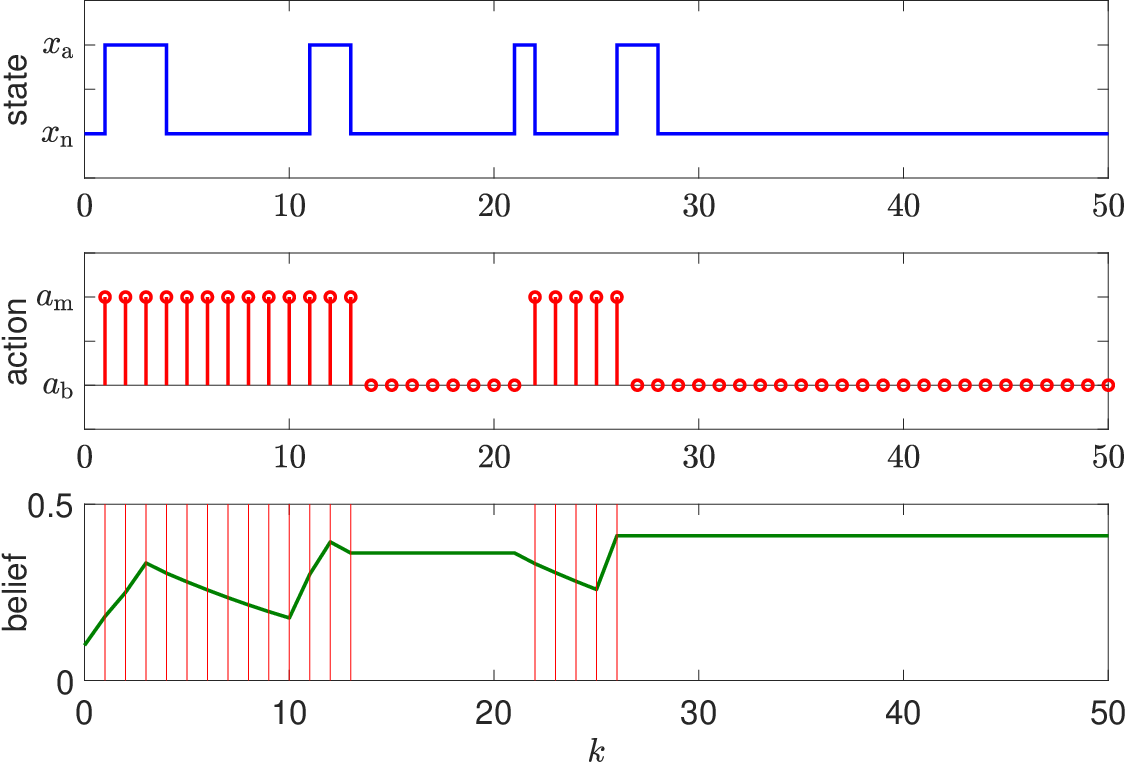
Under this setting, a sample path of the state, the action, and the belief on $\theta_{\rm m}$ for $\theta=\theta_{\rm m}$ is depicted in Fig. 5. The vertical lines in the graph of belief means the action at the time instant is $a_{\rm m}$. For $0\leq k\leq 12$, the belief is sufficiently small, and thus $a_{\rm m}$ is the rational action. For $13\leq k<21$, the belief is large, and hence $a_{\rm b}$ is taken when the state is $x_{\rm n}$. At $k=21$, the state is $x_{\rm a}$, and the belief begins to decrease. At $k=26$, the state is $x_{\rm n}$. Then the belief exceeds the threshold, and $a_{\rm b}$ regardless of the state is the rational action. This result coincides with Theorem 2. Note that, the reaction is always $r_{\rm b}$ when the belief is less than $0.5$, and hence the sender’s instantaneous utility depends only on the state and the receiver’s utility is one in this example.

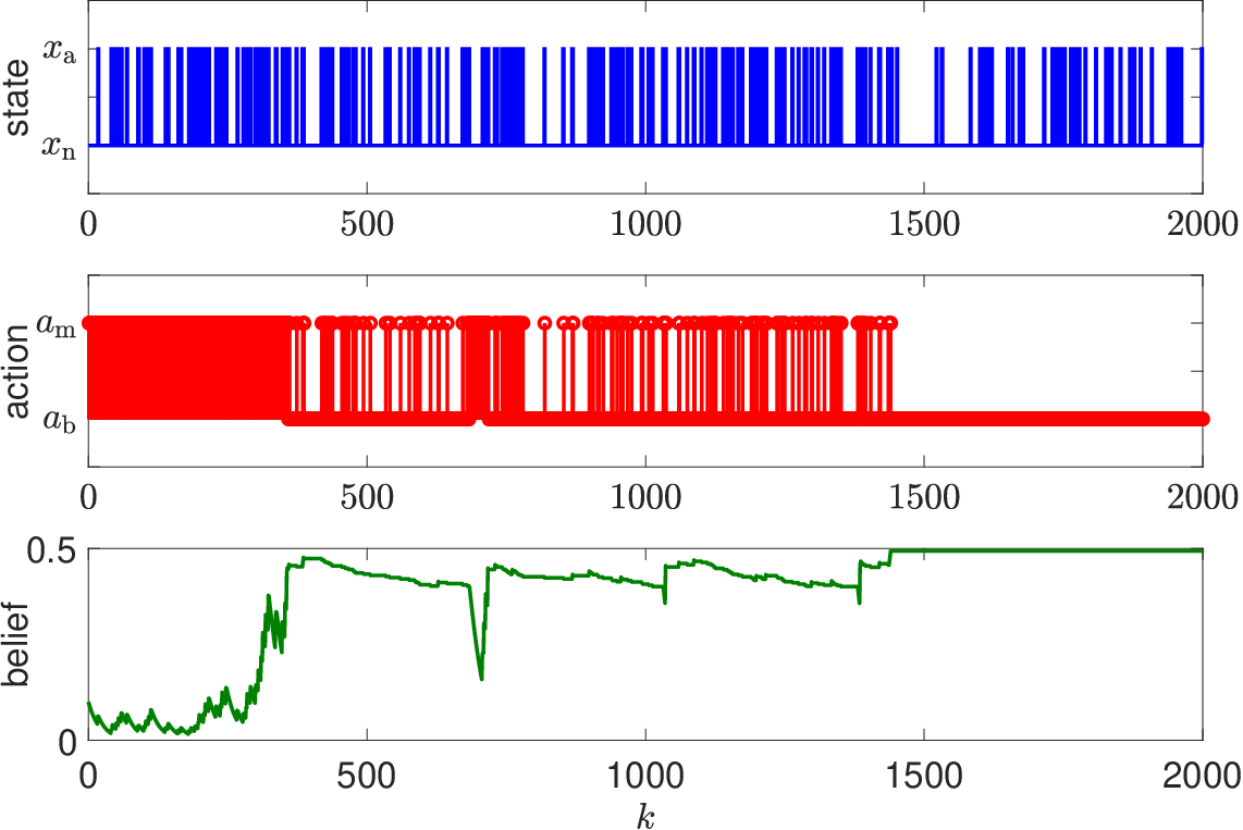
To investigate a long-term behavior, consider a situation where detection is more difficult. Specifically, the transition probability is given in Table III, which means the deviation of the transition probability by $a_{\rm m}$ is small. A sample path of the state, the action, and the belief on $\theta_{\rm m}$ for $\theta=\theta_{\rm m}$ is depicted in Fig. 6. Although the convergence speed is later than Fig. 5, the asymptotic security claim in Theorem 2 can be confirmed.

Roughly speaking, the result in Section III claims that the defender always wins in an asymptotic manner when the stochastic model of the control system is completely known and the vulnerability is known and modeled. The latter requirement is quantitatively described by the condition $\pi_{0}(\theta_{\rm m})>0$. Although the derived result claims a quite powerful defense capability, it is also true that it is almost impossible to be aware of all possible vulnerabilities in advance and to prepare appropriate counteraction for all scenarios.

As a practically interesting defense scheme, it may be possible to use the obtained property for passive bluffing. Suppose that the attacker does not know whether her attack scenario is supposed $(\pi_{0}(\theta_{\rm m})>0)$ or not $(\pi_{0}(\theta_{\rm m})=0)$. Also, imposing a certain property into the control system, we assume that state observation does not provide information about the reaction. For instance, the control system in the numerical example, where the behavior is independent of the reaction, satisfies this property. Under those assumptions, if the defender can conceal the actually conducted reactions, the true belief is completely unknown to the attacker. In this case, even if the attack is actually a zero-day attack through an unknown vulnerability $(\pi_{0}(\theta_{\rm m})=0)$, there is a possibility to be able to protect the control system. Specifically, if the attacker is risk-averse, i.e., she cares about the case $\pi_{0}(\theta_{\rm m})>0$, then she would possibly stop the attack after a while in a rational manner although the attack is unnoticed. Analysis of such passive bluffing utilizing the powerful detection capability achieved by model-based incident handling is a possible future direction.

References

- [1] N. Falliere, L. O. Murchu, and E. Chien, “W32. Stuxnet Dossier,” Symantec, Tech. Rep., 2011.
- [2] Cybersecurity & Infrastructure Security Agency, “Stuxnet malware mitigation,” Tech. Rep. ICSA-10-238-01B, 2014, [Online]. Available: https://www.us-cert.gov/ics/advisories/ICSA-10-238-01B.
- [3] ——, “Cyber-attack against Ukrainian critical infrastructure,” Tech. Rep. IR-ALERT-H-16-056-01, 2018, [Online]. Available: https://www.us-cert.gov/ics/alerts/IR-ALERT-H-16-056-01.
- [4] ——, “HatMan - safety system targeted malware,” Tech. Rep. MAR-17-352-01, 2017, [Online]. Available: https://www.us-cert.gov/ics/MAR-17-352-01-HatMan-Safety-System-Targeted-Malware-Update-B.
- [5] National Institute of Standards and Technology, “Guide for conducting risk assessments,” Tech. Rep. SP 800-30 Rev. 1, 2012.
- [6] P. Cichonski, T. Millar, T. Grance, and K. Scarfone, “Computer security incident handling guide,” National Institute of Standards and Technology, Tech. Rep. SP 800-61 Rev. 2, 2012, [Online]. Available: https://nvlpubs.nist.gov/nistpubs/SpecialPublications/NIST.SP.800-61r2.pdf.
- [7] J. Giraldo et al., “A survey of physics-based attack detection in cyber-physical systems,” ACM Comput. Surv., vol. 51, no. 4, 2018.
- [8] L. Xiao, X. Wan, X. Lu, Y. Zhang, and D. Wu, “IoT security techniques based on machine learning,” IEEE Signal Process. Mag., vol. 35, no. 5, pp. 41–49, 2018.
- [9] S. M. Dibaji, M. Pirani, D. B. Flamholz, A. M. Annaswamy, K. H. Johansson, and A. Chakrabortty, “A systems and control perspective of CPS security,” Annual Reviews in Control, vol. 47, pp. 394–411, 2019.
- [10] A. J. Gallo, M. S. Turan, F. Boem, T. Parisini, and G. Ferrari-Trecate, “A distributed cyber-Attack detection scheme with application to DC microgrids,” IEEE Trans. Autom. Control, vol. 65, no. 9, pp. 3800–3815, 2020.
- [11] M. Pajic, I. Lee, and G. J. Pappas, “Attack-resilient state estimation for noisy dynamical systems,” IEEE Trans. Control Netw. Syst., vol. 4, no. 1, pp. 82–92, 2017.
- [12] H. Sasahara, T. Ishizaki, J. Imura, and H. Sandberg, “Disconnection-aware attack detection and isolation with separation-based detector reconfiguration,” 2020, [Online]. Available: https://arxiv.org/abs/2009.11205.
- [13] T. E. Carroll and D. Grosu, “A game theoretic investigation of deception in network security,” Security and Communication Networks, vol. 4, no. 10, pp. 1162–1172, 2011.
- [14] F. Farokhi, A. M. H. Teixeira, and C. Langbort, “Estimation with strategic sensors,” IEEE Trans. Autom. Control, vol. 62, no. 2, pp. 724–739, 2017.
- [15] J. Pawlick, E. Colbert, and Q. Zhu, “Modeling and analysis of leaky deception using signaling games with evidence,” IEEE Trans. Inf. Forensics Security, vol. 14, no. 7, pp. 1871–1886, July 2019.
- [16] Q. Zhu and Z. Xu, Secure Estimation of CPS with a Digital Twin. Springer, 2020, pp. 115–138.
- [17] H. Sasahara, S. Sarıtaş, and H. Sandberg, “Asymptotic security of control systems by covert reaction: Repeated signaling game with undisclosed belief,” in Proc. 59th IEEE Conference on Decision and Control, 2020.
- [18] A. Rasekh, A. Hassanzadeh, S. Mulchandani, S. Modi, and M. K. Banks, “Smart water networks and cyber security,” Journal of Water Resources Planning and Management, vol. 142, no. 7, 2016.
- [19] E. Creaco, A. Campisano, N. Fontana, G. Marini, P. R. Page, and T. Walski, “Real time control of water distribution newtorks: A state-of-the-art review,” Water Research, vol. 161, pp. 517–530, 2019.
- [20] R. Taormina, S. Galelli, N. O. Tippenhauer, E. Salomons, and A. Ostfeld, “Characterizing cyber-physical attacks on water distribution systems,” Journal of Water Resources Planning and Management, vol. 143, no. 5, 2017.
- [21] P. Chen, L. Desmet, and C. Huygens, “A study on advanced persistent threats,” in Proc. International Conference on Communications and Multimedia Security, 2014, pp. 63–72.
- [22] R. S. Smith, “Covert misappropriation of networked control systems: Presenting a feedback structure,” IEEE Control Systems Magazine, vol. 35, no. 1, pp. 82–92, Feb. 2015.
- [23] A. Teixeira, I. Shames, H. Sandberg, and K. H. Johansson, “Revealing stealthy attacks in control systems,” in Proc. 50th Annual Allerton Conference on Communication, Control, and Computing, 2012, pp. 1806–1813.
- [24] F. Pasqualetti, F. Dörfler, and F. Bullo, “Control-theoretic methods for cyberphysical security: Geometric principles for optimal cross-layer resilient control systems,” IEEE Control Systems Magazine, vol. 35, no. 1, pp. 110–127, 2015.
- [25] R. Laraki, J. Renault, and S. Sorin, Mathematical Foundations of Game Theory, ser. Universitext. Springer, 2019.
- [26] P. Diaconis and D. Freedman, “On the consistency of bayes estimation,” Annals of Statistics, vol. 14, no. 1, pp. 1–26, 1986.
- [27] T. Sasaki, K. Sawada, S. Shin, and S. Hosokawa, “Model based fallback control for networked control system via switched Lyapunov function,” in Proc. 41st Annual Conference of the IEEE Industrial Electronics Society, 2015, pp. 2000–2005.
- [28] E. Çinlar, Probability and Statistics, ser. Graduate Texts in Mathematics. Springer, 2011.
- [29] R. Durrett, Probability: Theory and Examples, ser. Cambridge Series in Statistical and Probabilistic Mathematics. Cambridge University Press, 2019.