Identification at the Zero Lower Bound

Sophocles Mavroeidislabel=e1]sophocles.mavroeidis@economics.ox.ac.uk Email: [ Address: Department of Economics, University of Oxford

Abstract

I show that the Zero Lower Bound (ZLB) on interest rates can be used to identify the causal effects of monetary policy. Identification depends on the extent to which the ZLB limits the efficacy of monetary policy. I propose a simple way to test the efficacy of unconventional policies, modelled via a ‘shadow rate’. I apply this method to U.S. monetary policy using a three-equation structural vector autoregressive model of inflation, unemployment and the federal funds rate. I reject the null hypothesis that unconventional monetary policy has no effect at the ZLB, but find some evidence that it is not as effective as conventional monetary policy.

Keywords:

shadow rate,

keywords

\startlocaldefs\endlocaldefs

\support

This research is funded by the European Research Council via Consolidator grant number 647152. I would like to thank Guido Ascari, Sergio de Ferra, James Duffy, Andrea Ferrero, Jim Hamilton, Daisuke Ikeda, Federica Romei, Frank Schorheide, Francesco Zanetti and seminar participants at the Chicago Fed, New York Fed, Board of Governors, Bank of Japan, Hitotsubashi University, Keio University, UCL, University of Cambridge, University of Oxford, University of Warwick, DNB, University of Pennsylvania, Pennsylvania State University, NBER Summer Institute, IAAE conference, Netherlands Econometrics Study Group Meeting, World Congress and North American Winter meetings of the Econometric society for useful comments and discussion, as well as Mishel Ghassibe, Lukas Freund, Shangshang Li, and Patrick Vu for research assistance.

1 Introduction

The zero lower bound (ZLB) on nominal interest rates has arguably been a challenge for policy makers and researchers of monetary policy. Policy makers have had to resort to so-called unconventional policies, such as quantitative easing or forward guidance, which had previously been largely untested. Researchers have to use new theoretical and empirical methodologies to analyze macroeconomic models when the ZLB binds. So, the ZLB is generally viewed as a problem or at least a nuisance. This paper proposes to turn this problem on its head to solve another long-standing question in macroeconomics: the identification of the causal effects of monetary policy on the economy.

The intuition is as follows. If the ZLB limits the ability of policy makers to react to macroeconomic shocks, as argued, for example, by [9], the response of the economy to shocks will change when the policy instrument hits the ZLB. Because the difference in the behavior of macroeconomic variables across the ZLB and non-ZLB regimes is only due to the impact of monetary policy, the switch across regimes provides information about the causal effects of policy. In the extreme case that monetary policy completely shuts down during the ZLB regime, either because policy makers do not use alternative (unconventional) policy instruments, or because such instruments turn out to be completely ineffective, the only difference in the behavior of the economy across regimes is due to the impact of (conventional) policy during the unconstrained regime. Therefore, the ZLB identifies the causal effect of policy during the unconstrained regime. If monetary policy remains partially effective during the ZLB regime, e.g., through the use of unconventional policy instruments, then the difference in the behavior of the economy across regimes will depend on the difference in the effectiveness of conventional and unconventional policies. In this case, we obtain only partial identification of the causal effects of monetary policy, but we can still get informative bounds on the relative efficacy of unconventional policy. In the other extreme case that unconventional policy is as effective as conventional policy, there is no difference in the behavior of the economy across regimes, and we have no additional information to identify the causal effects of policy. However, we can still test this so-called ZLB irrelevance hypothesis (Debortoli et al. 2019) by testing whether the reaction of the economy to shocks is the same across the two regimes.

There are similarities between identification via occasionally binding constraints and identification through heteroskedasticity (Rigobon 2003), or more generally, identification via structural change (Magnusson and Mavroeidis 2014). That literature showed that the switch between different regimes generates variation in the data that identifies parameters that are constant across regimes. For example, an exogenous shift in a policy reaction function or in the volatility of shocks identifies the transmission mechanism, provided the latter is unaffected by the policy shift. When the switch from one regime to another is exogenous, regime indicators are valid instruments, and the methodology in Magnusson and Mavroeidis 2014 is applicable. However, regimes induced by occasionally binding constraints are not exogenous – whether the ZLB binds or not clearly depends on the structural shocks, so regime indicators cannot be used as instruments in the usual way, and a new methodology is needed to analyze these models.

In this paper, I show how to control for the endogeneity in regime selection and obtain identification in structural vector autoregressions (SVARs).¹¹ 1 There is a related literature on Dynamic Stochastic General Equilibrium (DSGE) models with a ZLB, see, e.g., Fernández-Villaverde et al. 2015, Guerrieri and Iacoviello 2015, Aruoba et al. 2017, Kulish et al. 2017 and Aruoba et al. 2020. The papers in this literature do not point out the implications of the ZLB for identification of monetary policy shocks. The methodology is parametric and likelihood-based, and the analysis is similar to the well-known Tobit model (Tobin 1958). More specifically, the methodological framework builds on the early microeconometrics literature on simultaneous equations models with censored dependent variables, see Amemiya 1974, Lee 1976, Blundell and Smith 1994, and the more recent literature on dynamic Tobit models, see Lee 1999, and particle filtering, see Pitt and Shephard 1999.

A further contribution of this paper is a general methodology to estimate reduced-form VARs with a variable subject to an occasionally binding constraint. This is a necessary starting point for SVAR analysis that uses any of the existing popular identification schemes, such as short- or long-run restrictions, sign restrictions, or external instruments. In the absence of any constraints, reduced-form VARs can be estimated consistently by Ordinary Least Squares (OLS), which is Gaussian Maximum Likelihood, or its corresponding Bayesian counterpart, and inference is fairly well-established. However, it is well-known that OLS estimation is inconsistent when the data is subject to censoring or truncation, see, e.g., Greene 1993 for a textbook treatment. So, it is not possible to estimate a VAR consistently by OLS using any sample that includes the ZLB, or even using (truncated) subsamples when the ZLB is not binding (because of selection bias), as was pointed out by Hayashi and Koeda 2019. It is not possible to impose the ZLB constraint using Markov switching models with exogenous regimes, as in Liu et al. 2019, because exogenous Markov-switching cannot guarantee that the constraint will be respected with probability one, and also does not account for the fact that the switch from one regime to the other depends on the structural shocks. Finally, it is not possible to perform consistent estimation and valid inference on the VAR (i.e., error bands with correct coverage on impulse responses), using externally obtained measures of the shadow rate, such as the one proposed by Wu and Xia 2016, as any such measures are subject to large and persistent estimation error that is not accounted for if they are treated as known in subsequent analysis. See also Rossi 2019 for a comprehensive discussion of the challenges posed by the ZLB for the estimation of structural VARs.

The methodology developed in this paper allows for the presence of a shadow rate, estimates of which can be obtained, but more importantly, it fully accounts for the impact of sampling uncertainty in the estimation of the shadow rate on inference about the structural parameters such as impulse responses. Therefore, the paper fills an important gap in the literature, as it provides the requisite methodology to implement any of the existing identification schemes. Hayashi and Koeda 2019 develop a VAR model with endogenous regime switching in which the policy variables that are subject to a lower bound are modelled using Tobit regressions. A key difference of their methodology from the one developed here is that they impose recursive identification of monetary policy shocks, which the present paper shows to be an overidentifying, and hence testable, restriction. Moreover, their model does not include shadow rates. A more recent paper by Aruoba et al. 2020 also studies SVARs with occasionally binding constraints, but does not focus on the implications of these constraints for identification.

Identification of the causal effects of policy by the ZLB does not require that the policy reaction function be stable across regimes. However, inference on the efficacy of unconventional policy, or equivalently, the causal effects of shocks to the shadow rate over the ZLB period, obviously depends on whether or not the reaction function remains the same across regimes. For example, an attenuation of the causal effects of policy over the ZLB period may indicate that unconventional policy is only partially effective, but it is also consistent with unconventional policy being less active (during ZLB regimes) than conventional policy (during non-ZLB regimes). This is a fundamental identification problem that is difficult to overcome without additional information, such as measures of unconventional policy stance, or additional identifying assumptions, such as parametric restrictions or external instruments. This can be done using the methodology developed in this paper.

The structure of the paper is as follows. Section 2 presents the main identification results of the paper in the context of a static bivariate simultaneous equations model with a limited dependent variable subject to a lower bound. Section 3 generalizes the analysis to a SVAR with an occasionally binding constraint and discusses identification, estimation and inference. Section 4 provides an application to a three-equation SVAR in inflation, unemployment and the Federal funds rate from Stock and Watson 2001. Using a sample of post-1960 quarterly US data, I find some evidence that the ZLB is empirically relevant, and that unconventional policy is only partially effective. Proofs and simulation results are given in the Appendix at the end.

2 Simultaneous equations model

I first illustrate the idea using a simple bivariate simultaneous equations model (SEM), which is both analytically tractable and provides a direct link to the related microeconometrics literature. To make the connection to the leading application, I will motivate this using a very stylized economy without dynamics in which the only outcome variable is inflation $\pi_{t}$ and the (conventional) policy instrument is the short-term nominal interest rate, $r_{t}$ . In addition to the traditional interest rate channel, the model allows for an ‘unconventional monetary policy’ channel that can be used when the conventional policy instrument hits the ZLB. An example of such a policy is quantitative easing (QE), in the form of long-term asset purchases by the central bank. Here I discuss a simple model of QE.²² 2 The more general SVAR model of the next section can also incorporate forward guidance in the form of Reifschneider and Williams 2000 and Debortoli et al. 2019, as shown in Ikeda et al. 2020.

Abstracting from dynamics and other variables, the equation that links inflation to monetary policy is given by

\pi_{t}=c+\beta\left(r_{t}-r^{n}\right)+\varphi b_{L,t}+\varepsilon_{1t},

(1)

where $c$ is a constant, $r^{n}$ is the neutral rate, $b_{L,t}$ is the amount of long-term bonds held by the private sector in log-deviation from its steady state, and $\varepsilon_{1t}$ is an exogenous structural shock unrelated to monetary policy. Equation (1) can be obtained from a model of bond-market segmentation, as in Chen et al. 2012, where a fraction of households is constrained to invest only in long-term bonds, see the Appendix for more details. In such a model, the parameter $\varphi$ that determines the effectiveness of QE is proportional to the fraction of constrained households and the elasticity of the term premium with respect to asset holdings, both of which are assumed to be outside the control of the central bank.

The nominal interest rate is set by a Taylor rule subject to the ZLB constraint, namely,


	$\displaystyle r_{t}$	$\displaystyle=\max\left(r_{t}^{\ast},0\right),$	(2a)
	$\displaystyle r_{t}^{\ast}$	$\displaystyle=r^{n}+\gamma\pi_{t}+\varepsilon_{2t},$	(2b)
where $r_{t}^{\ast}$ represents the desired target policy rate, and $\varepsilon_{2t}$ is a monetary policy shock. When $r_{t}^{\ast}$ is negative, it is unobserved. The unobserved $r_{t}^{\ast}$ will be referred to as the ‘shadow rate’, and it represents the desired policy stance prescribed by the Taylor rule in the absence of a binding ZLB constraint.

Suppose that QE is activated only when the conventional policy instrument $r_{t}$ hits the ZLB,³³ 3 The assumption that QE is only active during the ZLB regime is only made for simplicity, as it is inconsequential for the resulting functional form of the transmission equation. We can let QE be active all the time, and even allow for a different rule for QE above and below the ZLB, i.e., $b_{L,t}=\alpha\min\left(r_{t}^{\ast},0\right)+\alpha_{1}\max\left(r_{t}^{\ast},0\right)$ . Then, substituting back into (1) yields an equation that is isomorphic to (3), i.e., $\pi_{t}=\allowbreak c_{1}\allowbreak+\allowbreak\bar{\beta}r_{t}\allowbreak+\bar{\beta}^{\ast}\min\left(r_{t}^{\ast},0\right)\allowbreak+\varepsilon_{1t},$ with $\bar{\beta}:=\allowbreak\beta+\varphi\alpha_{1}$ and $\bar{\beta}^{\ast}\allowbreak:=\allowbreak\varphi\alpha.$ and follows the same policy rule (2b), up to a factor of proportionality $\alpha,$ i.e.,

b_{L,t}=\min\left(\alpha r_{t}^{\ast},0\right).

Substituting for $b_{L,t}$ in eq. (1) and letting $\beta^{\ast}:=\alpha\varphi$ , we obtain

\pi_{t}=c+\beta\left(r_{t}-r^{n}\right)+\beta^{\ast}\min\left(r_{t}^{\ast},0\right)+\varepsilon_{1t}.

(3)

A special case arises when QE is ineffective $\left(\varphi=0\right),$ or the monetary authority does not pursue a QE policy $\left(\alpha=0\right),$ so that eq. (3) becomes

\pi_{t}=c+\beta\left(r_{t}-r^{n}\right)+\varepsilon_{1t},

(4)

and monetary policy is completely inactive at the ZLB.

Another special case of the model given by equations (2) and (3) arises when $\beta^{\ast}=\beta$ in eq. (3). This happens when $\varphi\neq 0$ and $\alpha$ is chosen by the monetary authority to be equal to $\beta/\varphi.$ This can be done when policy makers know the transmission mechanism in eq. (1) and have no restrictions in setting the policy parameter $\alpha$ so as to fully remove the impact of the ZLB on conventional policy. In that case, the equation for the outcome variable becomes

\pi_{t}=c+\beta\left(r_{t}^{\ast}-r^{n}\right)+\varepsilon_{1t}.

(5)

The model given by equations (2) and (5) is one in which monetary policy is completely unconstrained and there is no difference in outcomes across policy regimes. Such models have been put forward by Swanson and Williams 2014, Debortoli et al. 2019 and Wu and Zhang 2019.

The nesting model given by eq. (3) allows the effects of conventional and unconventional policy to differ. This could reflect informational as well as political or institutional constraints that prevent policy makers from calibrating their unconventional policy response to match exactly the policy prescribed by the Taylor rule. For instance, it may be that policy makers do not know the effectiveness of the QE channel $\varphi$ , or that the scale of asset purchases needed to achieve the desired policy stance during a ZLB regime is too large to be politically acceptable. Such a consideration may be particularly pertinent, for example, in the Eurozone. Importantly, one does not need to take a theoretical stand on this issue, because the methodology that I develop in the paper can accommodate a wide range of possibilities, and, as I demonstrate below, the issue can be studied empirically.

To complete the specification of the model, I assume that the structural shocks $\varepsilon_{t}=\left(\varepsilon_{1t},\varepsilon_{2t}\right)^{\prime}$ are independently and identically distributed (i.i.d.) Normal with covariance matrix $\Sigma=diag\left(\sigma_{1}^{2},\sigma_{2}^{2}\right)$ .

The analysis in this paper assumes that the shadow rate $r_{t}^{*}$ is only observed above the ZLB. If $r^{*}_{t}<0$ were observed up to scale, for instance, if we could measure QE $b_{L,t}$ from the balance sheet of the central bank, then the computation of the likelihood would be much simpler – no filtering would be needed to deal with lags of $r_{t}^{\ast}<0$ on the right hand side of the SVAR model introduced in the next section, but the identification problem would remain the same. More generally, we could assume that $r_{t}^{\ast}<0$ is observed with some measurement error $\eta_{t}$ , and include the measurement equation $b_{L,t}=\min\left(\alpha r_{t}^{\ast}+\eta_{t},0\right)$ in the model together with a specification of the distribution of $\eta_{t}$ . The estimation method in this paper can then be seen as a special case where we are entirely agnostic about the measurement error. Adding such measures of unconventional policy is a potentially very useful extension of the method since, if correctly specified, they will likely improve estimation accuracy.

Connection to the microeconometrics literature Equations (2) and (3) form a SEM with a limited dependent variable. The special case with $\beta^{\ast}=0$ in (3) can be referred to as a kinked SEM (KSEM), while the opposite case of $\beta^{\ast}=\beta$ in (3) can be called a censored SEM (CSEM). Variants of the KSEM model have been studied in the early microeconometrics literature on limited dependent variable SEMs. Amemiya 1974 and Lee 1976 studied multivariate extensions of the well-known Tobit model (Tobin 1958). Nelson and Olson 1978 argued that the KSEM was less suitable for microeconometric applications than the CSEM, and the latter subsequently became the main focus of the literature (Smith and Blundell 1986; Blundell and Smith 1989). Blundell and Smith 1994 studied the unrestricted model using external instruments, so they did not consider the implications of the kink for identification.

One important lesson from the microeconometrics literature is that establishing existence and uniqueness of equilibria in this class of models is non-trivial. Gourieroux et al. 1980 define a model to be ‘coherent’ if it has a unique solution for the endogenous variables in terms of the exogenous variables, i.e., if there exists a unique reduced form. More recently, the literature has distinguished between existence and uniqueness of solutions using the terms coherency and completeness of the model, respectively (Lewbel 2007). Establishing coherency and completeness is a necessary first step before we can study identification and estimation.

2.1 Identification

Substituting for $r_{t}^{\ast}$ in (3) using (2) and rearranging, we obtain

	$\displaystyle\pi_{t}$	$\displaystyle=\widetilde{c}+\widetilde{\beta}\left(r_{t}-r^{n}\right)+\widetilde{\varepsilon}_{1t},\,\ \text{where}$		(6)
	$\displaystyle\widetilde{\beta}$	$\displaystyle=\frac{\beta-\beta^{\ast}}{1-\gamma\beta^{\ast}},\quad\widetilde{c}=\frac{c}{1-\gamma\beta^{}},\text{ and }\widetilde{\varepsilon}_{1t}=\frac{\varepsilon_{1t}+\beta^{}\varepsilon_{2t}}{1-\gamma\beta^{*}}.$		(7)

The system of equations (2) and (6) is now a KSEM, for which the necessary and sufficient condition for coherency and completeness (existence of a unique solution) is $\widetilde{\beta}\gamma<1$ (Nelson and Olson 1978). Using (7), the coherency and completeness condition can be expressed in terms of the structural parameters as

\frac{1-\gamma\beta}{1-\gamma\beta^{\ast}}>0.

(8)

This condition evidently restricts the admissible range of the structural parameters. It is satisfied in the present monetary policy model, where it is natural to assume that $\beta,\beta^{\ast}\leq 0$ and $\gamma>0$ . Therefore, it is possible that the coherency condition may not provide additional information relative to what is often available from natural sign restrictions on the parameters.

Under condition (8), the unique solution of the model can be written as

	$\displaystyle\pi_{t}$	$\displaystyle=\mu_{1}+u_{1t}-\widetilde{\beta}D_{t}\left(\mu_{2}+u_{2t}\right),\text{ and }$		(9)
	$\displaystyle r_{t}$	$\displaystyle=\max\left(\mu_{2}+u_{2t},0\right),$		(10)

where $D_{t}:=1_{\left\{r_{t}=0\right\}}$ is an indicator (dummy) variable that takes the value 1 when $r_{t}$ is on the boundary and zero otherwise, and

	$\displaystyle u_{1t}$	$\displaystyle=\frac{\widetilde{\varepsilon}_{1t}+\widetilde{\beta}\varepsilon_{2t}}{1-\gamma\widetilde{\beta}}=\frac{\varepsilon_{1t}+\beta\varepsilon_{2t}}{1-\gamma\beta},\quad u_{2t}=\frac{\gamma\varepsilon_{1t}+\varepsilon_{2t}}{1-\gamma\beta},$		(11)
	$\displaystyle\mu_{1}$	$\displaystyle=\frac{c}{1-\gamma\beta},\quad\mu_{2}=\frac{\gamma c}{1-\gamma\beta}+r^{n}.$

Equations (9) and (10) express the endogenous variables $\pi_{t},r_{t}$ in terms of the exogenous variables $\varepsilon_{1t},\varepsilon_{2t},$ and correspond to the decision rules of the agents in the model. It is clear that those decision rules differ in a world in which the ZLB occasionally binds, which is characterized by $\widetilde{\beta}\neq 0,$ compared to a world in which it never does (i.e., the CSEM), where $\widetilde{\beta}=0.$ What is important for identification, however, is that in a world in which the ZLB occasionally binds, agents’ reaction to shocks differs across regimes, and the difference depends on the parameter $\widetilde{\beta},$ which from eq. (7), depends on the difference between the impact of conventional and unconventional policies, $\beta$ and $\beta^{\ast},$ respectively. I will show that this change provides information that identifies the structural parameters: we get point identification when $\beta^{\ast}=0$ (the KSEM case), and partial identification when $\beta^{\ast}\neq\beta.$ The identification argument leverages the coefficient on the kink, $\widetilde{\beta},$ in the ‘incidentally kinked’ regression (9), which is identified by a variant of the well-known Heckit method (Heckman 1979). I will sketch out the argument below, and provide more details for the full SVAR model in the next section.

2.1.1 Identification of the KSEM

Recall that in the KSEM model $\widetilde{\beta}=\beta.$ Consider the estimation of $\beta$ in (4) from a regression of $\pi_{t}$ on $r_{t}$ using only observations above the ZLB,

E\left(\pi_{t}|r_{t},r_{t}>0\right)=c+\beta\left(r_{t}-r^{n}\right)+\rho\left(r_{t}-\mu_{2}+\tau\frac{\phi\left(a\right)}{1-\Phi\left(a\right)}\right),\quad a=\frac{-\mu_{2}}{\tau},

(12)

where $\rho=cov\left(u_{1t},u_{2t}\right)/\tau^{2}-\beta=\gamma\sigma_{1}^{2}\left(1-\gamma\beta\right)/\left(\gamma^{2}\sigma_{1}^{2}+\sigma_{2}^{2}\right)$ , $\tau=\sqrt{var\left(u_{2t}\right)},$ and $\phi\left(\cdot\right),$ $\Phi\left(\cdot\right)$ are standard Normal density and distribution functions, respectively. The coefficient $\rho$ is the bias in the estimation of $\beta$ from the truncated regression (12). Now, the mean of $\pi_{t}$ using the observations at the ZLB is

E\left(\pi_{t}|r_{t}=0\right)=c-\beta r^{n}+\rho\tau\frac{\phi\left(a\right)}{\Phi\left(a\right)}.

(13)

Next, observe that $\mu_{2},$ $\tau$ and hence $\phi\left(a\right)/\Phi\left(a\right)$ can be estimated from the Tobit regression (10). Therefore, we can recover the bias $\rho$ and identify $\beta.$ A simple way to implement this is the control function approach (Heckman 1978). Let

h_{t}\left(\mu_{2},\tau\right):=\left(1-D_{t}\right)\left(r_{t}-\mu_{2}\right)-D_{t}\frac{\tau\phi\left(a\right)}{\Phi\left(a\right)},

and run the regression

E\left(\pi_{t}|r_{t}\right)=c_{1}+\beta r_{t}+\rho h_{t}\left(\mu_{2},\tau\right),

(14)

where $c_{1}=c-\beta r^{n}$ is an unrestricted intercept. The rank condition for the identification of $\beta$ is simply that the regressors in (14) are not perfectly collinear. This holds if and only if $0<\Pr\left(D_{t}=1\right)<1.$ So, as long as some but not all the observations are at the boundary, the model is generically identified.

2.1.2 Partial identification of the unrestricted SEM

The discussion of the previous subsection shows that $\widetilde{\beta}$ is identified from the kink in the reduced-form equation for $\pi_{t}$ (9). It follows from eq. (7) and the order condition that $\beta,\beta^{*}$ are not point identified. I will now demonstrate that they are partially identified.

The assumption $cov\left(\varepsilon_{1t},\varepsilon_{2t}\right)=0$ implies (see proof of Proposition 3 for a derivation)

\gamma=\frac{\omega_{12}-\omega_{22}\beta}{\omega_{11}-\omega_{12}\beta}

(15)

where $\omega_{ij}:=cov\left(u_{it},u_{jt}\right)$ . Substituting for $\gamma$ in (7) using (15) yields

\widetilde{\beta}=\frac{\beta-\beta^{\ast}}{1-\frac{\omega_{12}-\omega_{22}\beta}{\omega_{11}-\omega_{12}\beta}\beta^{\ast}}.

(16)

For any given value of the reduced-form parameters $\widetilde{\beta},\Omega:=var(u_{t})$ , $u_{t}=(u_{1t},u_{2t})^{\prime}$ , the identified set for $\left(\beta,\beta^{\ast}\right)$ is a one-dimensional manifold in $\Re^{2}$ defined by eq. (16) intersected with the coherency condition (8).

It is instructive to illustrate the identified set graphically at some given value of $\widetilde{\beta}\,$ and $\Omega$ . Consider, for example, the case $\Omega$ equal to the identity $I_{2}$ , at which (15) yields $\gamma=-\beta,$ and the coherency condition (8) reduces to $1+\beta\beta^{\ast}>0,$ and (16) yields the function $\beta=\frac{\widetilde{\beta}+\beta^{\ast}}{1-\widetilde{\beta}\beta^{\ast}}$ . Figure 1 plots this function at $\widetilde{\beta}=-1/2$ . and highlights in dark gray the region of incoherency defined by $1+\beta\beta^{\ast}\leq 0$ . The identified set is the part of the function $\beta=\frac{\widetilde{\beta}+\beta^{\ast}}{1-\widetilde{\beta}\beta^{\ast}}$ that lies to the right of the pole at $1/\widetilde{\beta},$ i.e., in the region $\beta^{\ast}>1/\widetilde{\beta}=-2$ in this example.

Now, consider the additional restrictions $\beta\geq\beta^{\ast}\geq 0$ or $\beta\leq\beta^{\ast}\leq 0$ , highlighted by the light gray shaded areas in Figure 1. The interpretation of those restrictions is that unconventional policy neither has the opposite effect from conventional policy, nor is it more effective than conventional policy. With this additional restriction, we see that the identified set further shrinks to the part of $\beta=\frac{\widetilde{\beta}+\beta^{\ast}}{1-\widetilde{\beta}\beta^{\ast}}$ in the interval $(\widetilde{\beta}^{-1},0].$ The projection of the identified set onto the $\beta$ axis yields $\beta\in(-\infty,\widetilde{\beta}],$ since $\widetilde{\beta}<0$ , while its projection onto the $\beta^{\ast}$ axis yields $\beta^{\ast}\in$ $(\widetilde{\beta}^{-1},0]$ . Because equations (8) and (16) encapsulate all the information in the reduced-form parameters about $\beta,\beta^{\ast}$ , the identified set obtained from them is sharp.

Refer to caption — Figure 1: The identified set for $\left(\beta,\beta^{\ast}\right)$ when $\Omega=I$ and $\widetilde{\beta}=-1/2,$ obtained by the intersection of $\beta=\frac{\widetilde{\beta}+\beta^{\ast}}{1-\widetilde{\beta}\beta^{\ast}}$ and $1+\beta\beta^{\ast}>0$ (coherency condition). Light gray area corresponds to $\beta\leq\beta^{\ast}\leq 0$ and $\beta\geq\beta^{\ast}\geq 0$ . The thick part of the curve $\beta=\frac{\widetilde{\beta}+\beta^{\ast}}{1-\widetilde{\beta}\beta^{\ast}}$ indicates the identified set obtained from the combined restrictions, and the bold intervals on the axes give the projections of the identified set onto $\beta$ and $\beta^{\ast}$ .

Let us define a new parameter $\lambda$ such that $\beta^{*}=\lambda\beta$ . The restriction indicated by the light gray areas in Figure 1 corresponds to $\lambda\in\left[0,1\right]$ . If we interpret $\lambda$ as a measure of the efficacy of unconventional policy, this restriction implies that unconventional policy is neither counter- nor over-productive. This reparameterization offers a convenient way to discretize the parameter space when we compute the identified set numerically, as is the case in the more general model discussed in the next section.

In this bivariate model, it is possible to characterize the identified set analytically. Here, I discuss the identified set for $\beta$ and defer the discussion of $\lambda$ to Appendix A.1.

We have already established that $\beta$ is completely unidentified when $\beta=\beta^{*}$ (equivalently $\lambda=1$ ), which corresponds to the CSEM. From the definition of $\widetilde{\beta}$ in (7), it follows that $\beta=\beta^{*}$ implies $\widetilde{\beta}=0.$ So, when $\widetilde{\beta}=0$ , $\beta$ is completely unidentified. It remains to see what happens when $\widetilde{\beta}\neq 0$ . Let $\gamma_{0}:=\omega_{12}/\omega_{11}$ , which can be interpreted as the value the reaction function coefficient $\gamma$ in (2) would take if $\beta=0$ , i.e., the value corresponding to a Choleski identification scheme where $r_{t}$ is placed last. In Appendix A.1, I prove the following bounds

\widetilde{\beta}=0\text{ or }\widetilde{\beta}\gamma_{0}<0

, then

\beta\in\Re;

otherwise

\omega_{12}=\gamma_{0}=0

, then

\beta\in(-\infty,\widetilde{\beta}]

\widetilde{\beta}<0

\beta\in[\widetilde{\beta},\infty)

\widetilde{\beta}>0

;

\text{if }0<\widetilde{\beta}\gamma_{0}\leq 1,\text{ then }\beta\in\left[\frac{1}{\gamma_{0}},\widetilde{\beta}\right]

\widetilde{\beta}<0

\beta\in\left[\widetilde{\beta},\frac{1}{\gamma_{0}}\right]

\widetilde{\beta}>0

;

\widetilde{\beta}\gamma_{0}>1

, then

\lambda<0.

(17)

We see that when $\widetilde{\beta}\neq 0$ and $0\leq\widetilde{\beta}\gamma_{0}\leq 1$ , we can identify both the sign of the causal effect $\beta$ of $r_{t}$ on $\pi_{t}$ and get bounds on its magnitude. In particular, the identified coefficient $\widetilde{\beta}$ is an attenuated measure of the true causal effect $\beta$ . Moreover, $\widetilde{\beta}\gamma_{0}>1$ implies that $\beta^{\ast}$ has the opposite sign from $\beta$ , i.e., unconventional policy has the opposite effect of the conventional one. That could be interpreted as saying that unconventional policy is counterproductive.

Finally, the hypothesis that unconventional policy is as effective as conventional policy, $\beta^{*}=\beta$ or $\lambda=1$ , is equivalent to the null hypothesis $H_{0}:\widetilde{\beta}=0$ . The alternative that unconventional policy is less effective than conventional policy, $\beta>\beta^{\ast}$ if $\beta>0,$ or $\beta<\beta^{\ast}$ if $\beta<0$ , corresponds to the two-sided alternative $H_{1}:\widetilde{\beta}\neq 0$ . This can be tested using a likelihood ratio test.

3 SVAR with an occasionally binding constraint

I now develop the methodology for identification and estimation of SVARs with an occasionally binding constraint. Let $Y_{t}=\left(Y_{1t}^{\prime},Y_{2t}\right)^{\prime}$ be a vector of $k$ endogenous variables, partitioned such that the first $k-1$ variables $Y_{1t}$ are unrestricted and the $k$ th variable $Y_{2t}$ is bounded from below by $b$ .⁴⁴ 4 The lower bound does not need to be constant. All we need is to observe the periods in which the economy is at the ZLB regime. Define the latent process $Y_{2t}^{\ast}$ that is only observed, and equal to $Y_{2t},$ whenever $Y_{2t}>b$ . If $Y_{2t}$ is a policy instrument, $Y_{2t}^{\ast}$ can be thought of as the ‘shadow’ instrument that measures the desired policy stance. The $p$ th-order SVAR model is given by the equations

$\displaystyle A_{11}Y_{1t}+A_{12}Y_{2t}+A_{12}^{\ast}Y_{2t}^{\ast}$	$\displaystyle=B_{10}X_{0t}+\sum_{j=1}^{p}B_{1,j}Y_{t-j}+\sum_{j=1}^{p}B_{1,j}^{\ast}Y_{2,t-j}^{\ast}+\varepsilon_{1t},$	(18)
$\displaystyle A_{22}^{\ast}Y_{2t}^{\ast}+A_{22}Y_{2t}+A_{21}Y_{1t}$	$\displaystyle=B_{20}X_{0t}+\sum_{j=1}^{p}B_{2,j}Y_{t-j}+\sum_{j=1}^{p}B_{2,j}^{\ast}Y_{2,t-j}^{\ast}+\varepsilon_{2t},$	(19)
$\displaystyle Y_{2t}$	$\displaystyle=\max\left(Y_{2t}^{\ast},b\right),$

for $t\geq 1$ given a set of initial values $Y_{-s},Y_{2,-s}^{\ast},$ for $s=0,...,p-1$ , and $X_{0t}$ are exogenous and predetermined variables.

Equation (19) can be interpreted as a policy reaction function because it determines the desired policy stance $Y_{2t}^{\ast}.$ Similarly, $\varepsilon_{2t}$ is the corresponding policy shock. The above model is a dynamic SEM. Two important differences from a standard SEM are the presence of (i) latent lags amongst the predetermined variables on the right-hand side, which complicates estimation; and (ii) the contemporaneous value of $Y_{2t}$ in the policy reaction function (19), which allows it to vary across ZLB and non-ZLB regimes. The presence of latent lags $Y_{2,t-j}^{\ast}$ in the policy rule (19) is particularly useful because it allows the model to incorporate forward guidance (Reifschneider and Williams 2000; Debortoli et al. 2019), see Appendix D for details.

Collecting all the observed predetermined variables $X_{0t},Y_{t-1},...,Y_{t-p}$ into a vector $X_{t},$ and the latent lags $Y_{2,t-1}^{\ast},...,Y_{2,t-p}^{\ast}$ into $X_{t}^{\ast},$ and similarly for their coefficients, the model can be written compactly as:

	$\displaystyle\begin{pmatrix}A_{11}&A_{12}^{\ast}&A_{12}\\ A_{21}&A_{22}^{\ast}&A_{22}\end{pmatrix}\begin{pmatrix}Y_{1t}\\ Y_{2t}^{\ast}\\ Y_{2t}\end{pmatrix}$	$\displaystyle=BX_{t}+B^{\ast}X_{t}^{\ast}+\varepsilon_{t},$		(20)
	$\displaystyle Y_{2t}$	$\displaystyle=\max\left\{Y_{2t}^{\ast},b\right\}.$

The vector of structural errors $\varepsilon_{t}$ is assumed to be i.i.d. Normally distributed with zero mean and identity covariance.

In the previous section, we defined the KSEM as a special case of the general model, where $Y_{2t}^{\ast}<b$ has no (contemporaneous) impact on $Y_{1t}.$ In the dynamic setting, it feels natural to define the corresponding ‘kinked SVAR’ model (KSVAR) as a model in which $Y_{2t}^{\ast}$ has neither contemporaneous nor dynamic effects. Therefore, the KSVAR obtains as a special case of (20) when both $A_{12}^{\ast}=0,$ and $B^{\ast}=0,$ which corresponds to a situation in which the bound is fully effective in constraining what policy can achieve at all horizons.

The opposite extreme to the KSVAR is the censored SVAR model (CSVAR). Again, unlike the CSEM, which only characterizes contemporaneous effects, the idea of a CSVAR is to impose the assumption that the constraint is irrelevant at all horizons. So, it corresponds to a fully unrestricted linear SVAR in the latent process $\left(Y_{1t}^{\prime},Y_{2t}^{\ast}\right)^{\prime}$ . This is a special case of (20) when both $A_{12}=0$ and the elements of $B$ corresponding to lagged $Y_{2t}$ are equal to zero. Finally, I refer to the general model given by (20) as the ‘censored and kinked SVAR’ (CKSVAR).

Define the $k\times k$ square matrices

\overline{A}:=\begin{pmatrix}A_{11}&A_{12}+A_{12}^{\ast}\\ A_{21}&A_{22}+A_{22}^{\ast}\end{pmatrix},\text{ \ and \ }A^{\ast}:=\begin{pmatrix}A_{11}&A_{12}^{\ast}\\ A_{21}&A_{22}^{\ast}\end{pmatrix}.

(21)

$\overline{A}$ determines the impact effects of structural shocks during periods when the constraint does not bind. $A^{\ast}$ does the same for periods when the constraint binds.

To analyze the CKSVAR, we first need to establish existence and uniqueness of the reduced form. This is done in the following proposition.

Proposition 1

The model given in eq. (20) is coherent and complete (i.e., it has a unique solution) if and only if

\kappa:=\frac{\overline{A}_{22}-A_{21}A_{11}^{-1}\overline{A}_{12}}{A_{22}^{\ast}-A_{21}A_{11}^{-1}A_{12}^{\ast}}>0.

(22)

Note that (22) does not depend on the coefficients on the lags (whether latent or observed), so it is exactly the same as in a static SEM. This condition is useful for inference, e.g., when constructing confidence intervals or posteriors, because it restricts the range of admissible values for the structural parameters. It can also be checked empirically when the structural parameters are point-identified.

If condition (22) is satisfied, there exists a reduced-form representation of the CKSVAR model (20). For convenience of notation, define the indicator (dummy variable) that takes the value one if the constraint binds and zero otherwise:

D_{t}=1_{\left\{Y_{2t}=b\right\}}.

(23)

Proposition 2

If (22) holds, and for any initial values $Y_{-s},Y_{2,-s}^{\ast},$ $s=0,...,p-1,$ the reduced-form representation of (20) for $t\geq 1$ is given by

$\displaystyle Y_{1t}$	$\displaystyle=\overline{C}_{1}X_{t}+\overline{C}_{1}^{\ast}\overline{X}_{t}^{\ast}+u_{1t}-\widetilde{\beta}D_{t}\left(\overline{C}_{2}X_{t}+\overline{C}_{2}^{\ast}\overline{X}_{t}^{\ast}+u_{2t}-b\right)$	(24)
$\displaystyle Y_{2t}$	$\displaystyle=\max\left(\overline{Y}_{2t}^{\ast},b\right),$	(25)
$\displaystyle\overline{Y}_{2t}^{\ast}$	$\displaystyle=\overline{C}_{2}X_{t}+\overline{C}_{2}^{\ast}\overline{X}_{t}^{\ast}+u_{2t},$	(26)
$\displaystyle Y_{2t}^{\ast}$	$\displaystyle=\left(1-D_{t}\right)\overline{Y}_{2t}^{\ast}+D_{t}\left(\kappa\overline{Y}_{2t}^{\ast}+\left(1-\kappa\right)b\right),$	(27)

where $u_{t}=\left(u_{1t}^{\prime},u_{2t}\right)^{\prime}=\overline{A}^{-1}\varepsilon_{t},$ $\overline{C}^{\ast}=\left(\overline{C}_{1}^{\ast\prime},\overline{C}_{2}^{\ast\prime}\right)^{\prime}=\kappa\overline{A}^{-1}B^{\ast},$ $\overline{X}_{t}^{\ast}=\left(\overline{x}_{t-1},...,\overline{x}_{t-p}\right)^{\prime},$ $\overline{x}_{t}=\min\left(\overline{Y}_{2t}^{\ast}-b,0\right),$ $\overline{x}_{-s}=\kappa^{-1}\min\left(Y_{2,-s}^{\ast}-b,0\right),$ $s=0,...,p-1,$

\widetilde{\beta}=\left(A_{11}-A_{12}^{\ast}A_{22}^{\ast-1}A_{21}\right)^{-1}\left(A_{12}^{\ast}A_{22}^{\ast-1}A_{22}-A_{12}\right),

(28)

$\kappa$ is defined in (22) and the matrices $\overline{C}_{1},\overline{C}_{2},$ are given in eq. (49) in the Appendix.

Note that the “reduced-form” latent process $\overline{Y}_{2t}^{\ast}$ is, in general, different from the “structural” shadow rate $Y_{2t}^{\ast}$ defined by (27). They coincide only when $\kappa=1.$ This holds, for example, in the CSVAR model.

Equation (25) combined with (26) is a familiar dynamic Tobit regression model with the added complexity of latent lags included as regressors whenever $\overline{C}_{2}^{\ast}\neq 0.$ Likelihood estimation of the univariate version of this model was studied by Lee 1999. The $k-1$ equations (24) are ‘incidentally kinked’ dynamic regressions, that I have not seen analyzed before.

3.1 Identification

3.1.1 Identification of reduced-form parameters

Let $\psi$ denote the parameters that characterize the reduced form (24)-(25): $\widetilde{\beta},\overline{C},$ $\overline{C}^{\ast}$ and $\Omega=var\left(u_{t}\right).$ It is useful to decompose $\psi$ into $\psi_{2}=\left(\overline{C}_{2},\overline{C}_{2}^{\ast},\tau\right)^{\prime},$ where $\tau=\sqrt{var\left(u_{2t}\right)},$ and $\psi_{1}=(vec\left(\overline{C}_{1}\right)^{\prime},vec\left(\overline{C}_{1}^{\ast}\right)^{\prime},\allowbreak\widetilde{\beta}^{\prime},\delta^{\prime},vech\left(\Omega_{1.2}\right))^{\prime},$ where $\delta=\Omega_{12}/\tau^{2}$ , $\Omega_{1.2}=\Omega_{11}-\delta\delta^{\prime}\tau^{2}$ , and $\Omega_{ij}=cov\left(u_{it},u_{jt}\right)$ .

Equation (25) is the dynamic Tobit regression model studied by Lee 1999. So, its parameters, $\psi_{2},$ are generically identified provided that the regressors are not perfectly collinear. This requires that $0<\Pr\left(D_{t}=1\right)<1.$

Given $\psi_{2},$ the identification of the remaining parameters, $\psi_{1},$ can be characterized using a control function approach. Consider the $k-1$ regression equations

E\left(Y_{1t}|Y_{2t},X_{t},\overline{X}_{t}^{\ast}\right)=\overline{C}_{1}X_{t}+\overline{C}_{1}^{\ast}\overline{X}_{t}^{\ast}+\widetilde{\beta}Z_{1t}+\delta Z_{2t},

(29)

where

	$\displaystyle Z_{1t}$	$\displaystyle=D_{t}\left(b-\overline{C}_{2}X_{t}-\overline{C}_{2}^{\ast}\overline{X}_{t}^{\ast}-\frac{\tau\phi\left(a_{t}\right)}{\Phi\left(a_{t}\right)}\right),$		(30)
	$\displaystyle Z_{2t}$	$\displaystyle=\left(1-D_{t}\right)\left(Y_{2t}-\overline{C}_{2}X_{t}-\overline{C}_{2}^{\ast}\overline{X}_{t}^{\ast}\right)+D_{t}\frac{\tau\phi\left(a_{t}\right)}{\Phi\left(a_{t}\right)},$		(31)

$a_{t}=\left(\frac{b-\overline{C}_{2}X_{t}-\overline{C}_{2}^{\ast}\overline{X}_{t}^{\ast}}{\tau}\right)$ , and $\phi\left(\cdot\right),$ $\Phi\left(\cdot\right)$ are the standard Normal density and distribution functions, respectively. When $\overline{C}^{\ast}$ is different from zero, regressors $\overline{X}_{t}^{\ast}$ , $Z_{1t},$ and $Z_{2t}$ in (29) are unobserved, so we need to replace them with their expectations conditional on $Y_{2t},Y_{t-1},...,Y_{1}.$ Then, the regressors on the right-hand side of (29) become $\mathbf{X}_{t}:=\left(X_{t}^{\prime},\overline{X}_{t|t}^{\ast\prime},Z_{1t|t},Z_{2t|t}\right)^{\prime}$ , where $h_{t|t}:=E\left(h\left(\overline{X}_{t}^{\ast}\right)|Y_{2t},Y_{t-1},...,Y_{1}\right)$ for any function $h\left(\cdot\right)$ whose expectation exists.⁵⁵ 5 In the KSVAR model, we have $\overline{C}_{1}^{\ast}=0$ and $\overline{C}_{2}^{\ast}=0,$ so $\overline{X}_{t}^{\ast}$ drops out of (29), and the regressors $Z_{1t},Z_{2t}$ are observed, so $Z_{jt|t}=Z_{jt},$ $j=1,2.$ The coefficients $\overline{C}_{1},\overline{C}_{1}^{\ast},\widetilde{\beta},$ and $\delta$ are generically identified if the regressors $\mathbf{X}_{t}$ are not perfectly collinear.

3.1.2 Identification of structural parameters

From the order condition, we can easily establish that there are not enough restrictions to identify all the structural parameters in the CKSVAR (20). Let $k_{0}=\dim\left(X_{0t}\right)$ denote the number of predetermined variables other than the own lags of $Y_{t}.$ For example, in a standard VAR without deterministic trends, we have $X_{0t}=1,$ so $k_{0}=1.$ The number of reduced-form parameters $\psi$ is $k_{0}k+k^{2}p$ (in $\overline{C}$ ) plus $kp$ (in $\overline{C}^{\ast}$ ) plus $k-1$ (in $\widetilde{\beta}$ ) plus $k\left(k+1\right)/2$ (in $\Omega$ ). The number of structural parameters in (20) is $k_{0}k+k^{2}p$ (in $B$ ) plus $kp$ (in $B^{\ast}$ ) plus $k^{2}$ (in $\overline{A}$ ) plus $k$ (in $A_{12}^{\ast}$ and $A_{22}$ ). So, the CKSVAR is underidentified by $k\left(k-1\right)/2+1$ restrictions. Nevertheless, I will show that the impulse responses to $\varepsilon_{2t}$ are identified. Specifically, they are point-identified when $A_{12}^{\ast}=0,$ and partially identified when $A_{12}^{\ast}\neq 0$ but $A_{12}^{\ast}$ and $A_{12}$ have the same sign, analogous to the bounds given in equation (17) in the previous section.

Because the CKSVAR is nonlinear, IRFs are obviously state-dependent, and there are many ways one can define them, see Koop et al. 1996. The IRF to $\varepsilon_{2t},$ according to any of the definitions proposed in the literature, is identified if the reduced-form errors $u_{t}$ can be expressed as a known function of $\varepsilon_{2t}$ and a process that is orthogonal to it, i.e., $u_{t}=g\left(\varepsilon_{2t},e_{t}\right),$ where $e_{t}$ is independent of $\varepsilon_{2t}.$ From Proposition 2, it follows that the function $g$ is linear, and more specifically,

	$\displaystyle u_{1t}$	$\displaystyle=\left(I_{k-1}-\overline{\beta}\overline{\gamma}\right)^{-1}\left(\bar{\varepsilon}_{1t}+\overline{\beta}\bar{\varepsilon}_{2t}\right),\,\text{\ and}$		(32)
	$\displaystyle u_{2t}$	$\displaystyle=\left(1-\overline{\gamma}\overline{\beta}\right)^{-1}\left(\bar{\varepsilon}_{2t}+\overline{\gamma}\bar{\varepsilon}_{1t}\right),$		(33)

where

	$\displaystyle\overline{\beta}$	$\displaystyle:=-A_{11}^{-1}\overline{A}_{12},\quad\overline{\gamma}:=-\overline{A}_{22}^{-1}A_{21},$		(34)
	$\displaystyle\bar{\varepsilon}_{1t}$	$\displaystyle:=A_{11}^{-1}\varepsilon_{1t},\quad\bar{\varepsilon}_{2t}:=\overline{A}_{22}^{-1}\varepsilon_{2t},$

and $\overline{A}_{22}=A_{22}^{\ast}+A_{22},$ defined in (21). Note that $\overline{\beta}$ can be interpreted as the response of $Y_{1t}$ to a shock that increases $Y_{2t}$ by one unit, and $\overline{\gamma}$ are the contemporaneous reaction function coefficients of $Y_{2t}$ to $Y_{1t}$ when $Y_{2t}>b$ (unconstrained regime). The shock vector $\overline{\varepsilon}_{1t}$ is not structural but it is orthogonal to $\varepsilon_{2t},$ so it plays the role of $e_{t}$ in $u_{t}=g\left(\varepsilon_{2t},e_{t}\right).$ Hence, the IRF is identified if and only if $\overline{\beta},$ $\overline{\gamma},$ and $\overline{A}_{22}$ are identified.

The following proposition shows identification when $A_{12}^{\ast}=0$ .

Proposition 3

When $A_{12}^{\ast}=0$ and the coherency condition (22) holds, the parameters in (32)-(33) are identified by the equations $\overline{\beta}=\widetilde{\beta},$

	$\displaystyle\overline{\gamma}$	$\displaystyle=\left(\Omega_{12}^{\prime}-\Omega_{22}\overline{\beta}^{\prime}\right)\left(\Omega_{11}-\Omega_{12}\overline{\beta}^{\prime}\right)^{-1},\text{ and}$		(35)
	$\displaystyle\overline{A}_{22}^{-1}$	$\displaystyle=\sqrt{\left(-\overline{\gamma},1\right)\Omega\left(-\overline{\gamma},1\right)^{\prime}}.$		(36)

Remarks 1. $\overline{\beta}=\widetilde{\beta}$ follows immediately from the definition (28) with $A_{12}^{\ast}=0$ . Equations (35) and (36) hold without the restriction $A_{12}^{\ast}=0.$ They follow from the orthogonality of the shocks $\varepsilon_{2t}$ and $\overline{\varepsilon}_{1t}.$

2. An instrumental variables interpretation of this identification result is as follows. Define the instrument

Z_{t}:=Y_{1t}-\widetilde{\beta}Y_{2t}=A_{11}^{-1}B_{1}X_{t}+A_{11}^{-1}B_{1}^{\ast}X_{t}^{\ast}+A_{11}^{-1}\varepsilon_{1t},

where the second equality holds when $A_{12}^{\ast}=0$ . The orthogonality of the errors $E\left(\varepsilon_{1t}\varepsilon_{2t}\right)=0$ implies $E\left(Z_{t}\varepsilon_{2t}\right)=0.$ So, $Z_{t}$ are valid $k-1$ instruments for the $k-1$ endogenous regressors $Y_{1t}$ in the structural equation of $Y_{2t}=\max\left(Y_{2t}^{\ast},b\right)$ , where $Y_{2t}^{\ast}$ is given by (19). Normalizing (19) in terms of $Y_{2t}^{\ast}$ yields the structural equation in the more familiar form of a policy rule:

Y_{2t}=\max\left(\overline{\gamma}Y_{1t}+\bar{B}_{2}X_{t}+\bar{B}_{2}^{\ast}X_{t}^{\ast}+\bar{\varepsilon}_{2t},b\right),

(37)

where $\bar{B}_{2}=$ $\overline{A}_{22}^{-1}B_{2},$ $\bar{B}_{2}^{\ast}=$ $\overline{A}_{22}^{-1}B_{2}^{\ast}$ . Since $A_{11}^{-1}$ is non-singular, the coefficient matrix of $Z_{t}$ in the ‘first-stage’ regressions of $Y_{1t}$ is nonsingular, so the coefficients of (37) are generically identified by the rank condition. An alternative to the Tobit IV regression model (37) is the indirect Tobit regression approach used in the static SEM by Blundell and Smith 1994. Equation (37) can be written as the dynamic Tobit regression

Y_{2t}=\max\left(\widetilde{\gamma}Z_{t}+\tilde{B}_{2}X_{t}+\tilde{B}_{2}^{\ast}X_{t}^{\ast}+\tilde{\varepsilon}_{2t},b\right),

(38)

where $\widetilde{\gamma}=\left(1-\overline{\gamma}\overline{\beta}\right)^{-1}\overline{\gamma},$ $\tilde{B}_{2}=\left(1-\overline{\gamma}\overline{\beta}\right)^{-1}\bar{B}_{2},$ $\tilde{B}_{2}^{\ast}=\left(1-\overline{\gamma}\overline{\beta}\right)^{-1}\bar{B}_{2}^{\ast}$ and $\tilde{\varepsilon}_{2t}=\left(1-\overline{\gamma}\overline{\beta}\right)^{-1}\bar{\varepsilon}_{2t}.$ Note that the coherency condition (22) becomes $\kappa=\frac{\overline{A}_{22}}{A_{22}^{\ast}}\left(1-\overline{\gamma}\overline{\beta}\right)>0,$ so $1-\overline{\gamma}\overline{\beta}\neq 0,$ which guarantees the existence of the representation (38). Given $\overline{\beta}=\widetilde{\beta},$ the structural parameter $\overline{\gamma}$ can then be obtained as $\overline{\gamma}=\widetilde{\gamma}\left(I_{k-1}+\widetilde{\beta}\widetilde{\gamma}\right)^{-1},$ and similarly for the remaining structural parameters in (37).

3. The parameter $A_{22}$ allows the reaction function of $Y_{2t}^{\ast}$ to differ across the two regimes. The special case $A_{22}=0$ thus corresponds to the restriction that the reaction function remains the same across regimes. The parameters $A_{22}$ and $A_{22}^{\ast}$ are not separately identified. Hence, $A_{22}^{\ast-1}$ , the scale of the response to the shock $\varepsilon_{2t}$ during periods when $Y_{2t}=b$ , is not identified.⁶⁶ 6 This is akin to the well-known property of a probit model that the scale of the distribution of the latent process is not identifiable. Similarly, $\kappa=\frac{\overline{A}_{22}}{A_{22}^{\ast}}\left(1-\overline{\gamma}\overline{\beta}\right)$ is not identified, and therefore, neither is the structural shadow value $Y_{2t}^{\ast}$ in eq. (27). Identification of these requires an additional restriction on $A_{22}$ , e.g., $A_{22}=0.$ Turning this discussion around, we see that a change in the reaction function across regimes does not destroy the point identification of the effects of policy during the unconstrained regime, since the latter only requires $\overline{\beta},\overline{\gamma}$ and $\overline{A}_{22}$ , not $A_{22}^{\ast}$ or $\kappa.$

Next, we turn to the case $A_{12}^{\ast}\neq 0,$ and derive identification under restrictions on the sign and magnitude of $A_{12}^{\ast}$ relative to $A_{12}$ and $A_{22}^{\ast}$ relative to $A_{22}.$ The first restriction is motivated by a generalization of the discussion on the SEM model in Subsection 2.1.2. Specifically, if $\overline{A}_{12}=A_{12}+A_{12}^{\ast}$ measures the effect of conventional policy (operating in the unconstrained regime) and $A_{12}^{\ast}$ measures the effect of unconventional policy (operating in the constrained regime), then the assumption that $A_{12}$ and $A_{12}^{\ast}$ have the same sign means that unconventional policy effects are neither in the opposite direction nor larger in absolute value than conventional policy effects. In other words, unconventional policy is neither counterproductive nor over-productive relative to conventional policy. This can be characterized by the specification $A_{12}^{\ast}=\Lambda\overline{A}_{12}$ and $A_{12}=\left(I_{k-1}-\Lambda\right)\overline{A}_{12},$ where $\Lambda=diag\left(\lambda_{j}\right),$ $\lambda_{j}\in\left[0,1\right]$ for $j=1,...,k-1.$ I further impose the restriction that $\lambda_{j}=\lambda$ for all $j,$ so that $A_{12}^{\ast}=\lambda\overline{A}_{12}$ and $A_{12}=\left(1-\lambda\right)\overline{A}_{12}$ with $\lambda\in\left[0,1\right].$ This, in turn, means that $Y_{2t}$ and $Y_{2t}^{\ast}$ enter each of the first $k-1$ structural equations for $Y_{1t}$ only via the common linear combination $\lambda Y_{2t}^{\ast}\allowbreak+\allowbreak\left(1-\lambda\right)Y_{2t},$ which can be interpreted as a measure of the effective policy stance.

We also need to consider the impact of $A_{22}$ on identification. The parameter $\zeta=\overline{A}_{22}/A_{22}^{\ast}$ gives the ratio of the standard deviation of the monetary policy shock in the constrained relative to the unconstrained regime. It is also the ratio of the reaction function coefficients in the two regimes, e.g., $A_{22}^{\ast-1}A_{21}$ versus $\overline{A}_{22}^{-1}A_{21}$ . I will impose $\zeta>0,$ so that the sign of the policy shock does not change across regimes. With the above reparametrization and the definitions in (34), the identified coefficient $\widetilde{\beta}$ in (7) can be written as

\widetilde{\beta}=\left(1-\xi\right)\left(I-\xi\overline{\beta}\overline{\gamma}\right)^{-1}\overline{\beta},\quad\xi:=\lambda\zeta.

(39)

Similarly, given $\zeta>0,$ the coherency condition (22) reduces to $\left(1-\overline{\gamma}\overline{\beta}\right)\left(1-\xi\overline{\gamma}\overline{\beta}\right)>0.$ Notice that the parameters $\lambda,\zeta$ only appear multiplicatively, so it suffices to consider them together as $\xi=\lambda\zeta.$ Once $\overline{\beta}$ is known, the remaining structural parameters needed to obtain the IRF to $\varepsilon_{2t}$ are $\overline{\gamma}$ and $\overline{A}_{22}$ , and they are obtained from Proposition 3. So, the identified set can be characterized by varying $\xi$ over its admissible range. Without further restrictions on $\zeta,$ the admissible range is obviously $\xi\geq 0.$ If we further assume that $\zeta\leq 1,$ i.e., that the slope of the reaction function coefficients is no steeper in the constrained regime than in the unconstrained regime, then $\xi\in\left[0,1\right],$ and so partial identification proceeds exactly along the lines of the SEM in the previous section where $\lambda$ played the role of $\xi.$ In the case $k=2,$ the bounds derived in eq. (17) apply, with $\beta=\overline{\beta}$ in the notation of the present section. However, when $k>2,$ it is difficult to obtain a simple analytical characterization of the identified set for $\overline{\beta}.$ In any case, we will typically wish to obtain the identified set for functions of the structural parameters, such as the IRF. This can be done numerically by searching over a fine discretization of the admissible range for $\xi.$ An algorithm for doing this is provided in Appendix E.2.

3.2 Estimation

Estimation of the CKSVAR is carried out by Maximum Likelihood (ML) using either a version of the sequential importance sampler (SIS) of Lee 1999 or the fully adapted particle filter (FAPF) of Malik and Pitt 2011 to evaluate the likelihood, except in the case of the KSVAR model for which the likelihood is available analytically. The details are given in Appendix E.1.

Using the limit theory of Newey and McFadden 1994, the ML estimator can be shown to be consistent and asymptotically Normal and the LR statistic asymptotically $\chi^{2}$ with degrees of freedom equal to the number of restrictions. Standard asymptotics arise when the probability of each regime occurring is bounded away from zero. Infrequent visits to one of the two regimes will slow down the rate of convergence of the estimator, but will not lead to a non-standard limiting distribution. Since the focus of this paper is on identification, I will not discuss primitive conditions for these results, such as geometric ergodicity, which can be shown, for example, by bounding the joint spectral radius of the companion-form representation of the model (Liebscher 2005). Instead, I report Monte Carlo simulation results on the finite-sample properties of ML estimators and LR tests in Appendix B. They show that the Normal distribution provides a very good approximation to the finite-sample distribution of the ML estimators. I find some finite-sample size distortion in the LR tests of various restrictions on the CKSVAR, but this can be addressed effectively with a parametric bootstrap, as shown in the Appendix.

One interesting observation from the simulations is that the LR test of the CSVAR restrictions against the CKSVAR appears to be less powerful than the corresponding test of the KSVAR restrictions against the CKSVAR. Thus, we expect to be able to detect deviations from KSVAR more easily than deviations from CSVAR. In other words, finding evidence against the hypothesis that unconventional policies are fully effective (CSVAR) may be harder than finding evidence against the opposite hypothesis that they are completely ineffective (KSVAR).

4 Application

I use the three-equation SVAR of Stock and Watson 2001, consisting of inflation, the unemployment rate and the Federal Funds rate to provide a simple empirical illustration of the methodology developed in this paper. As discussed in Stock and Watson 2001, this model is far too limited to provide credible identification of structural shocks, so the results in this section are meant as an illustration of the new methods.

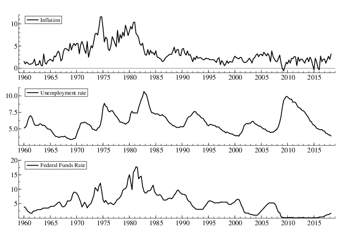
The data are quarterly and are constructed exactly as in Stock and Watson 2001.⁷⁷ 7 The inflation data are computed as $\pi_{t}=$ $400ln(P_{t}/P_{t-1})$ , where $P_{t}$ , is the implicit GDP deflator and $u_{t}$ is the civilian unemployment rate. Quarterly data on $u_{t}$ and $i_{t}$ are formed by taking quarterly averages of their monthly values. The variables are plotted in Figure 2 over the extended sample 1960q1 to 2018q2. I will consider all periods in which the Fed funds rate was below 20 basis points to be on the ZLB. This includes 28 quarters, or 11% of the sample.

4.1 Tests of efficacy of unconventional policy

I estimate three specifications of the SVAR(4) with the ZLB: the unrestricted CKSVAR specification, as well as the restricted KSVAR and CSVAR specifications. The maximum log-likelihood for each model is reported in Table 1, computed using the SIS algorithm in the case of CKSVAR and CSVAR, with 1000 particles. The accuracy of the SIS algorithm was gauged by comparing the log-likelihood to the one obtained using the resampling FAPF algorithm. In both CKSVAR and CSVAR the difference is very small. The results are also very similar when we increase the number of particles to 10000. Finally, the table reports the LR tests of KSVAR and CSVAR against CKSVAR using both asymptotic and parametric bootstrap p-values.

Table 1: Estimated CKSVAR models in Inflation, Unemployment and the Federal Funds rate\tabnoteref[a]tab1

Model	log lik	(FAPF)	# restr.	LR stat.	Asym. p-val.	Boot. p-val.
CKSVAR(4)	-81.64	-81.94
KSVAR(4)	-97.05	-	12	30.82	0.002	0.011
CSVAR(4)	-94.86	-94.87	14	26.43	0.023	0.117

\tabnotetext

[a]tab1Maximized log-likelihood of various SVAR models in inflation, unemployment and Federal funds rate. CKSVAR corresponds to the unrestricted specification (24)-(25); KSVAR excludes latent lags; CSVAR is a purely censored model. CKSVAR and CSVAR likelihoods computed using sequential importance sampling with 1000 particles (alternative estimates based on Fully Adapted Particle Filtering with resampling are shown in parentheses). Asymptotic p-values from $\chi^{2}_{q}$ , $q=$ number of restrictions. Bootstrap p-values from parametric bootstrap with 999 replications. Sample: 1960q1-2018q2 (234 obs, 11% at ZLB)

The KSVAR imposes the restriction that no latent lags (i.e., lags of the shadow rate) should appear on the right hand side of the model, i.e., $B^{\ast}=0$ in (20) or $\overline{C}_{1}^{\ast}=0$ and $\overline{C}_{2}^{\ast}=0$ in (24) and (25). This amounts to 12 exclusion restrictions on the CKSVAR(4), four restrictions in each of the three equations. This is necessary (but not sufficient) for the hypothesis that unconventional policy is completely ineffective at all horizons. It is necessary because $\overline{C}^{\ast}=\left(\overline{C}_{1}^{\ast\prime},\overline{C}_{2}^{\ast\prime}\right)^{\prime}\neq 0$ would imply that unconventional policy has at least a lagged effect on $Y_{t}.$ $\overline{C}^{\ast}=0$ is not sufficient to infer that unconventional policy is completely ineffective because it may still have a contemporaneous effect on $Y_{1t}$ if $A_{12}^{\ast}\neq 0,$ and the latter is not point-identified. The result of the test in Table 1 shows that lags of the shadow rate are statistically significant at the 5% level, rejecting the null hypothesis that unconventional policy has no effect.

The CSVAR model imposes the restriction that only the coefficients on the lags of the shadow rate (which is equal to the actual rate above the ZLB) are different from zero in the model, i.e., the elements of $B$ corresponding to lags of $Y_{2t}$ in (20) are all zero, or equivalently, the elements of $\overline{C}$ corresponding to lags of $Y_{2t}$ in (24) and (25) are all equal to $\overline{C}^{\ast}$ . In addition, it imposes the restriction that $\widetilde{\beta}=0$ in (24), i.e., no kink in the reduced-form equations for inflation and unemployment across regimes, yielding 14 restrictions in total. This is necessary for the hypothesis that the ZLB is empirically irrelevant for policy in that it does not limit what monetary policy can achieve. The evidence against this hypothesis is not as strong as in the case of the KSVAR. The asymptotic p-value is 0.023, indicating rejection of the null hypothesis that unconventional policy is as effective as conventional policy at the 5% level, but the bootstrap p-value is 0.117. Note that this difference could also be due to fact that the test of the CSVAR restrictions may be less powerful than the test of the KSVAR restrictions, as indicated by the simulations reported in the previous section. Thus, I would cautiously conclude that the evidence on the empirical relevance of the ZLB is mixed. Further evidence on the efficacy of unconventional policy will also be provided in the next subsection.

4.2 Impulse response functions

Based on the evidence reported in the previous section, I estimate the IRFs associated with the monetary policy shock using the unrestricted CKSVAR specification, and compare them to recursive IRFs from the CSVAR specification that place the Federal funds rate last in the causal ordering. From the identification results in Section 3, the CKSVAR point-identifies the nonrecursive IRFs only under the assumption that the shadow rate has no contemporaneous effect of $Y_{1t},$ i.e., $A_{12}^{\ast}=0$ in (18). Note that, due to the nonlinearity of the model, the IRFs are state-dependent. I use the following definition of the IRF from Koop et al. 1996:⁸⁸ 8 The kink in the reduced-form representation of the model makes it difficult to approximate the IRFs by local projections on simple nonlinear functions of the data, such as powers or interactions with the regime indicator, see Appendix E.3 for further discussion of this point.

IRF_{h,t}\left(\varsigma,X_{t},\overline{X}_{t}^{\ast}\right)=E\left(Y_{t+h}|\varepsilon_{2t}=\varsigma,X_{t},\overline{X}_{t}^{\ast}\right)-E\left(Y_{t+h}|\varepsilon_{2t}=0,X_{t},\overline{X}_{t}^{\ast}\right).

(40)

Figure 3 reports the nonrecursive IRFs to a 25 basis points monetary policy shock at the end of the sample, 2018q3 (at which point $\overline{X}_{t}^{\ast}=0$ in (40) because interest rates had been above the ZLB over the previous four quarters), from the CKSVAR under the assumption that unconventional policy has no contemporaneous effect ( $\lambda=0$ ). It also reports two different estimates of recursive IRFs using the identification scheme in Stock and Watson 2001 with interest rates placed last. The first estimate is obtained from the CSVAR specification, and the second is a “naive” OLS estimate of the IRF that ignores the ZLB constraint – a direct application of the method in Stock and Watson 2001 to the present sample. The figure also reports 90% bootstrap error bands for the nonrecursive IRFs.

In the nonrecursive IRF, the response of inflation to a monetary tightening is negative on impact, albeit very small, and, with the exception of the first quarter when it is positive, it stays negative throughout the horizon. Hence, the incidence of a price puzzle is mitigated relative to the recursive IRFs, according to which inflation rises for up to 6 quarters after a monetary tightening (9 quarters in the OLS case). Note, however, that the error bands are so wide that they cover (pointwise) most of the recursive IRF, though less so for the OLS one. Turning to the unemployment response, we see that the nonrecursive IRF starts significantly positive on impact (no transmission lag) and peaks much earlier (after 4 quarters) than the recursive IRF (10 quarters). In this case, the recursive IRF is outside the error bands for several quarters (more so for the naive OLS IRF). Finally, the response of the Federal funds rate to the monetary tightening is less than one on impact and generally significantly lower than the recursive IRFs. This is both due to the contemporaneous feedback from inflation and unemployment, as well as the fact that there is a considerable probability of returning to the ZLB, which mitigates the impact of monetary tightening.

Next, I turn to the identified sets of the IRFs that arise when I relax the restriction that unconventional policy is ineffective, i.e., $\lambda$ can be greater than zero. I consider the range of $\xi=\lambda\zeta\in\left[0,1\right],$ recalling that $\lambda$ measures the efficacy of unconventional policy and $\zeta$ measures the ratio of the reaction function coefficients and shock volatilities in the constrained versus the unconstrained regimes. The shaded areas in Figure 4 report the identified sets without any other restrictions. The striped areas (a subset of the aforementioned identified sets) show the tightening of the identified sets when I impose the additional sign restriction that the contemporaneous effect of the monetary policy shock to the Fed Funds rate should be nonnegative. The bold lines show the IRFs under the (point-identifying) assumption $\lambda=0$ . The latter are the same as the nonrecursive point estimates reported in Figure 3.

We observe that the identified set for the IRF of inflation is bounded from above by the limiting case $\lambda=0$ . This is also true of the response of the Fed Funds rate. The case $\lambda=0$ provides a lower bound on the effect to unemployment only from 0 to 9 quarters. Even though the point estimate of the unemployment response under $\lambda=0$ remains positive over all horizons, the identified set includes negative values beyond 10 quarters ahead. We also notice that the identified sets are fairly large, albeit still informative. Interestingly, the identified IRF of the Fed Funds rate includes a range of negative values on impact. These values arise because for values of $\xi>0$ , there are generally two solutions for the structural VAR parameters $\overline{\beta},\overline{\gamma}$ in the equations (35), (39), with one of them inducing such strong responses of inflation and unemployment to the interest rate that the contemporaneous feedback in the policy rule would in fact revert the direct positive effect of the policy shock on the interest rate. If we impose the additional sign restriction that the contemporaneous impact of the policy shock to the Fed Funds rate must be non-negative, then those values are ruled out and the identified sets become considerably tighter. This is an example of how sign restrictions can lead to tighter partial identification of the IRF.

With an additional assumption on $\zeta,$ the method can be used to obtain an estimate of the identified set for $\lambda,$ the measure of the efficacy of unconventional policy. In particular, if we set $\zeta=1,$ i.e., the reaction function remains the same across the two regimes, then the identified set for $\lambda$ is $\left[0.0.506\right].$ In other words, the identified set excludes values of the efficacy of policy beyond 51%, so that, roughly speaking, unconventional policy is at most 51% as effective as conventional one. Note that this estimate does not account for sampling uncertainty and relies crucially on the assumption that the reaction function remains the same across the two regimes. This assumption could be justified by arguing that there is no reason to believe that policy objectives may have shifted over the ZLB period, and that any desired policy stance was feasible over that period. The latter assumption may be questionable. For example, one can imagine that there may be financial and political constraints on the amount of quantitative easing policy makers could do, which may cause them to proceed more cautiously over the ZLB period than over regular times. Within the context of our model, this would be reflected as a flatter policy reaction function over the ZLB period than over the non-ZLB periods, i.e., it will correspond to $\zeta<1$ . To illustrate the implications of this for the identification of $\lambda$ , suppose that $\zeta=1/2,$ i.e., the shadow rate reacts half as fast to shocks during the ZLB period than it does in the non-ZLB period. Then, the identified set for $\lambda$ would include 1, i.e., the data would be consistent with the view that unconventional policy is fully effective. So, under this alternative assumption on $\zeta$ , the reason we observed a subdued response to policy shocks over the ZLB period is because policy was less active over that period, and policy shocks were smaller, not because unconventional policy was partially ineffective.

As I discussed in the introduction, it is difficult to make further progress on this issue without further information or additional assumptions. The technical reason is that the scale of the latent regression over the censored sample is not identified, so additional information is required to untangle the structural parameters $\lambda$ and $\zeta$ from $\xi=\lambda\zeta$ . One possibility would be to identify $\lambda$ from the coefficients on the lags of $Y_{2t}$ and $Y_{2t}^{\ast}$ by imposing the (overidentifying) restriction that $Y_{2t-j}$ and $Y_{2t-j}^{\ast}$ appear in the model only via the linear combination $Y_{2t-j}^{\text{eff}}:=\lambda Y_{2t-j}^{\ast}\allowbreak+\allowbreak\left(1-\lambda\right)\allowbreak Y_{2t-j}$ for all lags $j=1,...,p,$ where $Y_{2t}^{\text{eff}}$ can be interpreted as the effective policy stance. Provided that the coefficients on the lags of $Y_{2t}^{\ast}$ or $Y_{2t}$ are not all zero, this restriction point identifies $\lambda,$ and hence, partially identifies $\zeta$ from $\xi.$ One could obtain tighter bounds by using sign restrictions (Ikeda et al. 2020, see), or obtain point identification by using conventional identification schemes. For instance, one can identify $\overline{\beta}$ directly using external instruments, as in Gertler and Karadi 2015, and hence point identify $\xi$ from (39).

5 Conclusion

This paper has shown that the ZLB can be used constructively to identify the causal effects of monetary policy on the economy. Identification relies on the (in)efficacy of alternative (unconventional) policies. When unconventional policies are partially effective in mitigating the impact of the ZLB, the causal effects of monetary policy are only partially identified. A general method is proposed to estimate SVARs subject to an occasionally binding constraint. The method can be used to test the efficacy of unconventional policy, modelled via a shadow rate. Application to a core three-equation SVAR with US data suggests that the ZLB is empirically relevant and unconventional policy is only partially effective.

Appendix A Proofs

A.1 Derivation of identified set for model of Section 2

Using the notation $\beta^{*}=\lambda\beta$ , eq. (16) can be expressed as

\widetilde{\beta}=g\left(\beta\right)\beta,\text{\quad}g\left(\beta\right):=\frac{1-\lambda}{1-\lambda\frac{\beta\left(\omega_{12}-\omega_{22}\beta\right)}{\omega_{11}-\omega_{12}\beta}}.

(41)

When $\omega_{12}=0,$ we have $g\left(\beta\right)=$ $\frac{1-\lambda}{1+\lambda\omega_{22}\beta^{2}/\omega_{11}}\in\left(0,1\right)$ for all $\lambda\in\left(0,1\right).$ Therefore, when $\widetilde{\beta}\neq 0,$ the sign of $\beta$ is the same as that of $\widetilde{\beta}$ and its magnitude is lower, as stated in (17).

Next, consider $\omega_{12}\neq 0.$ It is easily seen that $g\left(0\right)=1-\lambda$ and $\lim_{\beta\rightarrow\pm\infty}\left(\beta\right)=0.$ Moreover,

\frac{\partial g}{\partial\beta}=\lambda\left(1-\lambda\right)\frac{\omega_{12}\omega_{22}\beta^{2}-2\omega_{11}\omega_{22}\beta+\omega_{11}\omega_{12}}{\left(\omega_{11}-\beta\omega_{12}-\beta\lambda\omega_{12}+\beta^{2}\lambda\omega_{22}\right)^{2}}.

For $\lambda\in\left(0,1\right),$ the above derivative function has zeros at $\omega_{12}\omega_{22}\beta^{2}-2\omega_{11}\omega_{22}\beta+\omega_{11}\omega_{12}=0$ , which occur at

\begin{array}[c]{c}\beta_{1}=\frac{\omega_{11}\omega_{22}+\sqrt{\omega_{11}\omega_{22}\left(\omega_{11}\omega_{22}-\omega_{12}^{2}\right)}}{\omega_{12}\omega_{22}}\\ \beta_{2}=\frac{\omega_{11}\omega_{22}-\sqrt{\omega_{11}\omega_{22}\left(\omega_{11}\omega_{22}-\omega_{12}^{2}\right)}}{\omega_{12}\omega_{22}}\end{array},\quad\text{if }\omega_{12}\neq 0.

Now, because $0<\left(\omega_{11}\omega_{22}-\omega_{12}^{2}\right)<\omega_{11}\omega_{22}$ implies $\sqrt{\omega_{11}\omega_{22}\left(\omega_{11}\omega_{22}-\omega_{12}^{2}\right)}<\omega_{11}\omega_{22},$ we have $\beta_{i}<0,$ $i=1,2,$ when $\omega_{12}<0$ and $\beta_{i}>0,$ $i=1,2,$ when $\omega_{12}>0.$

By symmetry, it suffices to consider only one of the two cases, e.g., the case $\omega_{12}<0.$ In this case, $g^{\prime}\left(\beta\right)=\frac{\partial g}{\partial\beta}<0$ for all $\beta>0$ and, since $g\left(0\right)=1-\lambda$ and $g\left(\infty\right)=0,$ it follows that $g\left(\beta\right)\in\left(0,1-\lambda\right)$ for all $\beta>0.$ Thus, from (41) we see that $\widetilde{\beta}<0$ cannot arise from $\beta>0$ when $\omega_{12}<0.$ In other words, observing $\widetilde{\beta}<0$ must mean that $\beta<0.$ Moreover, since $g^{\prime}\left(\beta\right)<0$ for all $\beta>\beta_{1}$ and $\beta_{1}<0,$ it must be that $g\left(\beta\right)>0$ for all $\beta>\beta_{1},$ and hence, also for $\beta_{1}<\beta\leq 0.$ At $\beta<\beta_{1},$ $g^{\prime}\left(\beta\right)>0,$ and since $g^{\prime}\left(\beta\right)<0$ for all $\beta<\beta_{2}<\beta_{1},$ and $g\left(-\infty\right)=0,$ it has to be that $g\left(\beta\right)$ approaches zero from below as $\beta\rightarrow-\infty,$ and therefore, $g\left(\beta\right)$ must cross zero at some $\beta_{0}\in\left(\beta_{2},\beta_{1}\right),$ and $g\left(\beta\right)\geq 0$ for all $\beta\in\left[\beta_{0},0\right].$ Inspection of (41) shows that $\beta_{0}=\omega_{11}/\omega_{12}=1/\gamma_{0},$ which corresponds to $\gamma=-\infty$ from (15). Since $g\left(\beta\right)\in\left[0,1-\lambda\right]$ for all $\beta\in\left[\beta_{0},0\right],$ and $\lambda\in(0,1),$ it follows from (41) that $\left|\widetilde{\beta}\right|\leq\left|\beta\right|$ . In other words, $\widetilde{\beta}$ is attenuated relative to the true $\beta.$

Finally, we notice that there is a minimum value of $\widetilde{\beta}$ that one can observe under the restriction $\lambda\in\left[0,1\right]$ (at $\lambda=1,$ $\widetilde{\beta}=0$ ). Given the attenuation bias and the fact that $\widetilde{\beta}<0$ if and only if $\beta\in\left[\beta_{0},1\right],$ the smallest value of $\widetilde{\beta}$ occurs when $\lambda=0$ and $\beta=\omega_{11}/\omega_{12},$ so $\widetilde{\beta}_{\min}=\omega_{11}/\omega_{12}=1/\gamma_{0}$ . Thus, observing $\widetilde{\beta}<\omega_{11}/\omega_{12}$ and $\omega_{12}<0,$ or $\widetilde{\beta}\omega_{12}/\omega_{11}>1,$ violates the identifying restriction that $\lambda\geq 0$ , for only with a $\lambda<0$ can we get $g\left(\beta\right)>1$ when $\beta<0$ and hence $\widetilde{\beta}<\beta<0$ .

A.1.1 Bounds on $\lambda$

The bounds on $\lambda$ are obtained by finding all the values of $\lambda$ for which equation (41) has a solution for $\beta$ . This equation implies

\beta^{2}\left(\left(1-\lambda\right)\omega_{12}+\widetilde{\beta}\lambda\omega_{22}\right)-\beta\left(\left(1-\lambda\right)\omega_{11}+\widetilde{\beta}\left(1+\lambda\right)\omega_{12}\right)+\widetilde{\beta}\omega_{11}=0,

whose discriminant is the following quadratic function of lambda:

\displaystyle D\left(\lambda\right)

\displaystyle=\left(\left(1-\lambda\right)\omega_{11}+\widetilde{\beta}\left(1+\lambda\right)\omega_{12}\right)^{2}-4\widetilde{\beta}\omega_{11}\left(\left(1-\lambda\right)\omega_{12}+\widetilde{\beta}\lambda\omega_{22}\right).

Hence, the identified set for $\lambda$ corresponds to $S_{\lambda}=\left\{\lambda:D\left(\lambda\right)\geq 0\right\}$ . This set is non-empty because $D\left(0\right)\geq 0.$ It can be computed analytically and can take the following three shapes: (i) $S_{\lambda}=\Re$ if $D\left(\lambda\right)\allowbreak\geq\allowbreak 0$ for all $\lambda\in\Re$ ; (ii) $S_{\lambda}\allowbreak=\allowbreak(-\infty,\lambda_{lo}]\allowbreak\cup\allowbreak[\lambda_{up},\infty)$ if $\omega_{11}\allowbreak-\allowbreak\widetilde{\beta}\omega_{12}\allowbreak\neq\allowbreak 0,$ where $\lambda_{lo}<\lambda_{up}$ are the roots of $D\left(\lambda\right)=0$ ; and (iii) $S_{\lambda}\allowbreak=\allowbreak(-\infty,\lambda_{lo}]$ if $\omega_{11}\allowbreak-\allowbreak\widetilde{\beta}\omega_{12}\allowbreak=\allowbreak 0,$ because $\omega_{11}^{2}\allowbreak-\allowbreak\left(\frac{\omega_{11}}{\omega_{12}}\right)^{2}\allowbreak\omega_{12}^{2}\allowbreak-\allowbreak 2\left(\frac{\omega_{11}}{\omega_{12}}\right)\allowbreak\omega_{11}\omega_{12}\allowbreak+\allowbreak 2\left(\frac{\omega_{11}}{\omega_{12}}\right)^{2}\allowbreak\omega_{11}\omega_{22}\allowbreak=\allowbreak 2\omega_{11}^{2}\allowbreak\frac{\omega_{11}\omega_{22}-\omega_{12}^{2}}{\omega_{12}^{2}}\allowbreak>\allowbreak 0$ . If we also impose the restriction $\lambda\in\left[0,1\right],$ then the identified set is $S_{\lambda}\cap\left[0,1\right]$ .

A.2 Proof of Proposition 1

Define $\overline{A}_{i2}:=A_{i2}^{\ast}+A_{i2},$ $i=1,2$ as the right blocks of $\overline{A}$ that was defined in (21). Applying (Gourieroux et al. 1980, Theorem 1), coherency holds if and only if $\det\overline{A}$ and $\det A^{\ast}$ have the same sign. Without loss of generality, we can assume that $A_{11}$ is nonsingular (this can always be achieved by reordering the variables in $Y_{t}$ ). From (21), we have $\det A^{\ast}=\det A_{11}\det\left(A_{22}^{\ast}-A_{21}A_{11}^{-1}A_{12}^{\ast}\right)$ and $\det\overline{A}=\det A_{11}\det\left(\overline{A}_{22}-A_{21}A_{11}^{-1}\overline{A}_{12}\right)$ (Lütkepohl 1996, p. 50 (6)). The coherency condition can be written as $\det\overline{A}/\det A^{\ast}>0,$ which, given that $\left(\overline{A}_{22}-A_{21}A_{11}^{-1}\overline{A}_{12}\right)$ and $\left(A_{22}^{\ast}-A_{21}A_{11}^{-1}A_{12}^{\ast}\right)$ are scalars, yields (22).

A.3 Proof of Proposition 2

Define $\overline{A}_{i2}:=A_{i2}^{\ast}+A_{i2},$ $i=1,2$ as the right blocks of $\overline{A}$ that was defined in (21). Also let $Y_{t}^{\ast}:=\left(Y_{1t}^{\prime},Y_{2t}^{\ast}\right)^{\prime}.$ When the coherency condition (22) holds, the solution of (20) exists and is unique. It can be expressed as

Y_{t}^{\ast}=\left\{\begin{array}[c]{ll}CX_{t}+C^{\ast}X_{t}^{\ast}+u_{t},&\text{if }D_{t}=0\\ \widetilde{C}X_{t}+\widetilde{C}^{\ast}X_{t}^{\ast}+\widetilde{c}b+\widetilde{u}_{t},&\text{if }D_{t}=1\end{array}\right.

(42)

where

C=\overline{A}^{-1}B,\quad C^{\ast}=\overline{A}^{-1}B^{\ast},\quad u_{t}=\overline{A}^{-1}\varepsilon_{t}

(43)

and

\widetilde{C}=A^{\ast-1}B,\quad\widetilde{C}^{\ast}=A^{\ast-1}B^{\ast},\quad\widetilde{c}=-A^{\ast-1}\binom{A_{12}}{A_{22}}b,\quad\widetilde{u}_{t}=A^{\ast-1}\varepsilon_{t}.

(44)

Using the partitioned inverse formula, we obtain

	$\displaystyle\widetilde{C}_{1}$	$\displaystyle=\left(A_{11}-A_{12}^{\ast}A_{22}^{\ast-1}A_{21}\right)^{-1}\left(B_{1}-A_{12}^{\ast}A_{22}^{\ast-1}B_{2}\right)$
	$\displaystyle\widetilde{C}_{2}$	$\displaystyle=\left(A_{22}^{\ast}-A_{21}A_{11}^{-1}A_{12}^{\ast}\right)^{-1}\left(B_{2}-A_{21}A_{11}^{-1}B_{1}\right)$

and

	$\displaystyle C_{1}$	$\displaystyle=\left(A_{11}-\overline{A}_{12}\overline{A}_{22}^{-1}A_{21}\right)^{-1}\left(B_{1}-\overline{A}_{12}\overline{A}_{22}^{-1}B_{2}\right)$
	$\displaystyle C_{2}$	$\displaystyle=\left(\overline{A}_{22}-A_{21}A_{11}^{-1}\overline{A}_{12}\right)^{-1}\left(B_{2}-A_{21}A_{11}^{-1}B_{1}\right).$

Solving the latter for $B_{1}$ and $B_{2}$ yields

B_{1}=A_{11}C_{1}+\overline{A}_{12}C_{2},\text{ and }B_{2}=\overline{A}_{22}C_{2}+A_{21}C_{1}\text{.}

Thus,

	$\displaystyle\widetilde{C}_{1}$	$\displaystyle=C_{1}+\left(A_{11}-A_{12}^{\ast}A_{22}^{\ast-1}A_{21}\right)^{-1}\left(\overline{A}_{12}-A_{12}^{\ast}A_{22}^{\ast-1}\overline{A}_{22}\right)C_{2}=C_{1}-\widetilde{\beta}C_{2},\text{ and}$
	$\displaystyle\widetilde{C}_{2}$	$\displaystyle=\left(A_{22}^{\ast}-A_{21}A_{11}^{-1}A_{12}^{\ast}\right)^{-1}\left(A_{22}^{\ast}-A_{21}A_{11}^{-1}A_{12}^{\ast}+A_{22}-A_{21}A_{11}^{-1}A_{12}\right)C_{2}=\kappa C_{2},$

where $\kappa$ is given in (22). The exact same derivations apply to $\widetilde{C}^{\ast},$ i.e.,

\widetilde{C}_{1}^{\ast}=C_{1}^{\ast}-\widetilde{\beta}C_{2}^{\ast},\text{ \ and \ }\widetilde{C}_{2}^{\ast}=\kappa C_{2}^{\ast}.

Next,

	$\displaystyle\widetilde{c}_{1}$	$\displaystyle=\left(A_{11}-A_{12}^{\ast}A_{22}^{\ast-1}A_{21}\right)^{-1}\left(A_{12}^{\ast}A_{22}^{\ast-1}A_{22}-A_{12}\right)b=\widetilde{\beta}b,\text{ and}$
	$\displaystyle\widetilde{c}_{2}$	$\displaystyle=-\frac{A_{22}-A_{21}A_{11}^{-1}A_{12}}{A_{22}^{\ast}-A_{21}A_{11}^{-1}A_{12}^{\ast}}b=\left(1-\kappa\right)b.$

Finally, $\widetilde{u}_{t}=A^{\ast-1}\overline{A}u_{t}=\left(\widetilde{u}_{1t}^{\prime},\widetilde{u}_{2t}\right)^{\prime}$ , where

\widetilde{u}_{1t}=u_{1t}-\widetilde{\beta}u_{2t},\text{ and \ }\widetilde{u}_{2t}=\kappa u_{2t}.

Substituting back into (42), the reduced-form model for $Y_{1t}$ becomes

	$\displaystyle Y_{1t}$	$\displaystyle=\left(1-D_{t}\right)\left(C_{1}X_{t}+C_{1}^{\ast}X_{t}^{\ast}+u_{1t}\right)$
		$\displaystyle+D_{t}\left(\left(C_{1}-\widetilde{\beta}C_{2}\right)X_{t}+\left(C_{1}^{\ast}-\widetilde{\beta}C_{2}^{\ast}\right)X_{t}^{\ast}+u_{1t}-\widetilde{\beta}u_{2t}\right),$		(45)

and for $Y_{2t}^{\ast}$ it is

Y_{2t}^{\ast}=C_{2}X_{t}+C_{2}^{\ast}X_{t}^{\ast}+u_{2t}-\left(1-\kappa\right)D_{t}\left(C_{2}X_{t}+C_{2}^{\ast}X_{t}^{\ast}+u_{2t}-b\right).

(46)

Next, define

\widetilde{Y}_{2t}^{\ast}:=C_{2}X_{t}+C_{2}^{\ast}X_{t}^{\ast}+u_{2t},

(47)

and rewrite (46) as

	$\displaystyle Y_{2t}^{\ast}$	$\displaystyle=\widetilde{Y}_{2t}^{\ast}-\left(1-\kappa\right)D_{t}\left(\widetilde{Y}_{2t}^{\ast}-b\right)$
		$\displaystyle=\left(1-D_{t}\right)\widetilde{Y}_{2t}^{\ast}+D_{t}\left(\kappa\widetilde{Y}_{2t}^{\ast}+\left(1-\kappa\right)b\right).$		(48)

Let $q=\dim X_{t}$ denote the number of elements of $X_{t}$ and define, for each $i=1,2,$

\overline{C}_{ij}=\left\{\begin{array}[c]{ll}C_{ij},&j\in\left\{1,q\right\}:X_{tj}\neq Y_{2,t-s}\text{ for all }s\in\left\{1,p\right\}\\ C_{ij}+C_{is}^{\ast},&j\in\left\{1,q\right\}:X_{tj}=Y_{2,t-s},\text{ for some }s\in\left\{1,p\right\}.\end{array}\right.

(49)

In other words, $\overline{C}$ contains the original coefficients on all the regressors other than the lags of $Y_{2t},$ while the coefficients on the lags of $Y_{2t}$ are augmented by the corresponding coefficients of the lags of $Y_{2t}^{\ast}.$ For example, if $p=1$ and there are no other exogenous regressors $X_{0t},$ then, for $i=1,2,$

C_{i}X_{t}+C_{i}^{\ast}X_{t}^{\ast}=C_{i1}Y_{1t-1}+C_{i2}Y_{2t-1}+C_{i}^{\ast}Y_{2t-1}^{\ast},

so $\overline{C}_{i}=\left(C_{i1},C_{i2}+C_{i}^{\ast}\right)$ . Using (49), we can rewrite (47) as

\widetilde{Y}_{2t}^{\ast}=\overline{C}_{2}X_{t}+C_{2}^{\ast}\min\left(X_{t}^{\ast}-b,0\right)+u_{2t}.

(50)

Now, observe that

\min\left(Y_{2t}^{\ast}-b,0\right)=D_{t}\left(Y_{2t}^{\ast}-b\right)=\kappa D_{t}\left(\widetilde{Y}_{2t}^{\ast}-b\right)=\kappa\min\left(\widetilde{Y}_{2t}^{\ast}-b,0\right)

So, letting $\widetilde{X}_{t}^{\ast}$ denote the lags of $\widetilde{Y}_{2t}^{\ast},$ we have $\min\left(X_{t}^{\ast}-b,0\right)=\kappa\min\left(\widetilde{X}_{t}^{\ast}-b,0\right),$ and consequently,

C^{\ast}\min\left(X_{t}^{\ast}-b,0\right)=\overline{C}^{\ast}\min\left(\widetilde{X}_{t}^{\ast}-b,0\right),

where $\overline{C}^{\ast}=\kappa C^{\ast}.$ Now, from (50) we have

\widetilde{Y}_{2t}^{\ast}=\overline{C}_{2}X_{t}+\overline{C}_{2}^{\ast}\min\left(\widetilde{X}_{t}^{\ast}-b,0\right)+u_{2t}.

Recall the definition of $\overline{Y}_{2t}^{\ast}$ in (26):

\overline{Y}_{2t}^{\ast}:=\overline{C}_{2}X_{t}+\overline{C}_{2}^{\ast}\overline{X}_{t}^{\ast}+u_{2t},

where $\overline{X}_{t}^{\ast}:=\left(\overline{x}_{t-1},...,\overline{x}_{t-p}\right)^{\prime},$ and $\overline{x}_{t}\allowbreak:=\allowbreak\min\left(\overline{Y}_{2t}^{\ast}\allowbreak-b,0\right),$ with initial conditions $\overline{x}_{-s}\allowbreak=\kappa^{-1}\allowbreak\min\left(Y_{2,-s}^{\ast}\allowbreak-b,0\right),$ $s=0,...,\allowbreak p-1.$ It follows that $\min\left(\widetilde{X}_{t}^{\ast}-b,0\right)\allowbreak=\overline{X}_{t}^{\ast}$ for all $t\geq 1,$ so that $\widetilde{Y}_{2t}^{\ast}=\overline{Y}_{2t}^{\ast}.$ Substituting $\overline{Y}_{2}^{\ast}$ for $\widetilde{Y}_{2}^{\ast}$ in (48), we get (27). Using the reparametrization (49) and the relationship between $X_{t}^{\ast}$ and $\overline{X}_{t}^{\ast}$ in (45), we obtain (24).

Finally, from eq. (46), it follows that the event $Y_{2t}^{\ast}<b$ is equivalent to

b+\kappa\left(C_{2}X_{t}+C_{2}^{\ast}X_{t}^{\ast}+u_{2t}-b\right)<b,

which, since $\kappa>0$ by the coherency condition (22), is equivalent to

u_{2t}<b-C_{2}X_{t}-C_{2}^{\ast}X_{t}^{\ast}.

(51)

Using the definition (26), and (49), the inequality (51) can be written as $\overline{Y}_{2t}^{\ast}<b,$ which establishes (25).

Comment: Note that $\kappa$ appears in the reduced form only multiplicatively with $C^{\ast},$ so $\kappa$ and $C^{\ast}$ are not separately identified, only $\overline{C}^{\ast}=\kappa C^{\ast}$ is. The reparametrization from $C$ to $\overline{C}$ is convenient because $\overline{C}$ is identified independently of $\kappa,$ while $C,C^{\ast}$ and $\kappa$ are not separately identified.

A.4 Proof of Proposition 3

We solve $u_{t}=\overline{A}^{-1}\varepsilon_{t}$ using the partitioned inverse formula to get

	$\displaystyle u_{1t}$	$\displaystyle=\left(A_{11}-\overline{A}_{12}\overline{A}_{22}^{-1}A_{21}\right)^{-1}\left(\varepsilon_{1t}-\overline{A}_{12}\overline{A}_{22}^{-1}\varepsilon_{2t}\right)$		(52)
	$\displaystyle u_{2t}$	$\displaystyle=\left(\overline{A}_{22}-A_{21}A_{11}^{-1}\overline{A}_{12}\right)^{-1}\left(\varepsilon_{2t}-A_{21}A_{11}^{-1}\varepsilon_{1t}\right).$		(53)

Using the definitions

	$\displaystyle\overline{\beta}$	$\displaystyle:=-A_{11}^{-1}\overline{A}_{12},\quad\overline{\gamma}:=-\overline{A}_{22}^{-1}A_{21},$
	$\displaystyle\bar{\varepsilon}_{1t}$	$\displaystyle:=A_{11}^{-1}\varepsilon_{1t},\quad\bar{\varepsilon}_{2t}:=\overline{A}_{22}^{-1}\varepsilon_{2t},$

we can rewrite (52)-(53) as (32)-(33).

Note that

	$\displaystyle\bar{\varepsilon}_{1t}$	$\displaystyle=A_{11}^{-1}\left(A_{11}u_{1t}+\overline{A}_{12}u_{2t}\right)=u_{1t}-\bar{\beta}u_{2t},$
	$\displaystyle\bar{\varepsilon}_{2t}$	$\displaystyle=\overline{A}_{22}^{-1}\left(A_{21}u_{1t}+\overline{A}_{22}u_{2t}\right)=-\overline{\gamma}u_{1t}+u_{2t},$

so,

	$\displaystyle var\left(\bar{\varepsilon}_{1t}\right)$	$\displaystyle=\left(I_{k-1},-\bar{\beta}\right)\Omega\left(I_{k-1},-\bar{\beta}\right)^{\prime},$
	$\displaystyle var\left(\bar{\varepsilon}_{2t}\right)$	$\displaystyle=\left(-\bar{\gamma},1\right)\Omega\left(-\bar{\gamma},1\right)^{\prime},$

and

	$\displaystyle cov\left(\bar{\varepsilon}_{1t},\bar{\varepsilon}_{2t}\right)$	$\displaystyle=\left(I_{k-1},-\overline{\beta}\right)\begin{pmatrix}\Omega_{11}&\Omega_{12}\\ \Omega_{12}^{\prime}&\Omega_{22}\end{pmatrix}\left(-\overline{\gamma},1\right)^{\prime}$
		$\displaystyle=-\left(\Omega_{11}-\overline{\beta}\Omega_{12}^{\prime}\right)\overline{\gamma}^{\prime}+\Omega_{12}-\overline{\beta}\Omega_{22}=0.$

The last equation identifies $\overline{\gamma}$ given $\overline{\beta}$ . Specifically,

\overline{\gamma}^{\prime}=\left(\Omega_{11}-\overline{\beta}\Omega_{12}^{\prime}\right)^{-1}\left(\Omega_{12}-\overline{\beta}\Omega_{22}\right).

Appendix B Numerical results

This section provides Monte-Carlo evidence on the finite-sample properties of the proposed estimators and tests. The data generating process (DGP) is a trivariate VAR(1), given by equations (18) and (19). I consider three different DGPs corresponding to the CKSVAR, KSVAR and CSVAR models, respectively. In all three DGPs, the following parameters are set to the same values: the contemporaneous coefficients are $A_{11}=I_{2},$ $A_{12}=$ $A_{12}^{\ast}=0_{2\times 1},$ $A_{22}^{\ast}=1$ and $A_{22}=0;$ the intercepts are set to zero, $B_{10}=0_{2\times 1}$ and $B_{20}=0;$ the coefficients on the lags are $B_{1,1}=\left(\rho I_{2},0\right),$ $B_{1,1}^{\ast}=0_{2\times 1},$ $B_{2,1}=\left(0_{1\times 2},B_{22,1}\right)$ , with $\rho=0.5.$ Finally, each of the three DGPs is determined as follows. DGP1: $B_{22,1}=B_{2,1}^{\ast}=0$ (both KSVAR and CSVAR restrictions hold, since lags of $Y_{2,t}$ and $Y_{2,t}^{\ast}$ all have zero coefficients); DGP2: $B_{22,1}=\rho,\,B_{2,1}^{\ast}=0\$ (KSVAR restrictions hold but CSVAR restrictions do not); DGP3: $B_{22,1}=0,\,B_{2,1}^{\ast}=\rho$ (CSVAR restrictions hold but KSVAR restrictions do not). The setting of the autoregressive coefficient $\rho=0.5$ leads to a lower degree of persistence than is typically observed in macro data (e.g., in the Stock and Watson, 2001, application, the three largest roots are 0.97, 0.97 and 0.8), because I want to avoid confounding any possible finite-sample issues arising from the ZLB with well-known problems of bias and size distortion due to strong persistence (near unit roots) in the data. Finally, the bound on $Y_{2t}$ is set to $b=0,$ the sample size is $T=250,$ the initial conditions are set to 0 and the number of Monte Carlo replications is 1000. In all cases, the CKSVAR and CSVAR likelihoods are computed using SIS with $R=1000$ particles. The notation for the reported parameters is given in Table 2.

Table 2: Parameter notation in reported simulation results

Mnemonic	Description
$\tau$	st. dev. of reduced form error $u_{2t}$ in $Y_{2t}$ (constrained variable)
Eq. 3	reduced form equation for $Y_{2t}$
Eq. j	red. form equation for $Y_{1j,t},$ $j=1,2$ (unconstrained variables)
$\widetilde{\beta}_{j}$	coefficient on kink in eq. j
eq. i Y1j_1	coefficient of $Y_{1j,t-1}$ in eq. i
eq. i Y2_1	coefficient of $Y_{2,t-1}$ in eq. i
eq. i lY2_1	coefficient of $\min\left(Y_{2,t-1}^{\ast}-b,0\right)$ in eq. i
$\delta_{j}$	coefficient of regression of $u_{1j,t}$ (red. form error in Eq. j) on $u_{2t}$
Ch_ij	(i,j) element of Choleski factor of $\Omega_{1.2}$

Figure 5 reports the sampling distribution of the ML estimators of the reduced-form parameters in Proposition 2 for the CKSVAR model under DGP1. The results for the KSVAR and CSVAR models, which are also correctly specified under DGP1, are omitted because they are entirely analogous. The sampling densities appear to be very close to the superimposed Normal approximations, indicating that the Normal asymptotic approximation is fairly accurate.

Table 3 reports moments of the sampling distributions of the above mentioned estimators for the CKSVAR model. Again, the results for the KSVAR and CSVAR models are entirely analogous and are therefore omitted. We notice no discernible biases. Additional simulation results with $T=100$ and $T=1000$ given in the Tables 4, 5 and 6 indicate that the RMSE declines at rate $\sqrt{T}$ in accordance with asymptotic theory. It is noteworthy that the estimators of $\widetilde{\beta}$ have substantially larger RMSE than the estimators of the other parameters.

Table 3: Moments of sampling distribution of ML estimators of the parameters of CKSVAR(1)\tabnoteref[a]tab2

ML-CKSVAR	true	mean	bias	sd	RMSE
$\tau$	1.000	0.983	-0.017	0.068	0.070
Eq.3 Constant	0.000	-0.006	-0.006	0.175	0.176
Eq.3 Y11_1	0.000	0.000	0.000	0.061	0.061
Eq.3 Y12_1	0.000	-0.000	-0.000	0.064	0.064
Eq.3 Y2_1	0.000	-0.010	-0.010	0.173	0.173
Eq.3 lY2_1	0.000	-0.013	-0.013	0.258	0.258
$\tilde{\beta}_{1}$	-0.000	-0.008	-0.008	0.356	0.356
$\tilde{\beta}_{2}$	0.000	-0.004	-0.004	0.359	0.359
Eq.1 Constant	0.000	0.002	0.002	0.213	0.213
Eq.1 Y11_1	0.500	0.489	-0.011	0.057	0.058
Eq.1 Y12_1	0.000	0.002	0.002	0.060	0.060
Eq.1 Y2_1	0.000	-0.002	-0.002	0.163	0.163
Eq.2 Constant	0.000	0.005	0.005	0.214	0.214
Eq.2 Y11_1	0.000	0.000	0.000	0.058	0.058
Eq.2 Y12_1	0.500	0.491	-0.009	0.057	0.058
Eq.2 Y2_1	0.000	-0.001	-0.001	0.159	0.159
Eq.1 lY2_1	0.000	0.005	0.005	0.232	0.232
Eq.2 lY2_1	0.000	0.002	0.002	0.233	0.233
$\delta_{1}$	0.000	-0.001	-0.001	0.157	0.157
$\delta_{2}$	0.000	-0.004	-0.004	0.155	0.155
Ch_11	1.000	0.975	-0.025	0.044	0.051
Ch_21	0.000	-0.001	-0.001	0.066	0.066
Ch_22	1.000	0.972	-0.028	0.046	0.054

\tabnotetext

[a]tab2Computed under DGP1 with $T=250$ using 1000 MC replications. Parameter names described in Table 2.

Table 4: Bias, standard deviation and Root Mean Square Error of Maximum Likelihood estimator of parameters of CKSVAR(1) model\tabnoteref[a]tab4

ML-CKSVAR	$T=100$			$T=250$			$T=1000$
Parameter	bias	sd	RMSE	bias	sd	RMSE	bias	sd	RMSE
$\tau$	-0.048	0.111	0.121	-0.017	0.068	0.070	-0.003	0.035	0.035
Eq.3 Constant	0.001	0.293	0.293	-0.006	0.175	0.176	0.004	0.085	0.085
Eq.3 Y11_1	-0.001	0.111	0.111	0.000	0.061	0.061	0.000	0.032	0.032
Eq.3 Y12_1	-0.004	0.109	0.109	-0.000	0.064	0.064	-0.000	0.031	0.031
Eq.3 Y2_1	-0.031	0.289	0.291	-0.010	0.173	0.173	-0.003	0.082	0.082
Eq.3 lY2_1	-0.022	0.435	0.436	-0.013	0.258	0.258	0.003	0.122	0.122
$\tilde{\beta}_{1}$	0.012	0.586	0.586	-0.008	0.356	0.356	0.000	0.176	0.176
$\tilde{\beta}_{2}$	-0.011	0.606	0.606	-0.004	0.359	0.359	-0.003	0.168	0.168
Eq.1 Constant	0.000	0.360	0.360	0.002	0.213	0.213	0.007	0.105	0.105
Eq.1 Y11_1	-0.034	0.098	0.104	-0.011	0.057	0.058	-0.002	0.029	0.029
Eq.1 Y12_1	-0.004	0.108	0.108	0.002	0.060	0.060	0.001	0.028	0.028
Eq.1 Y2_1	-0.004	0.281	0.281	-0.002	0.163	0.163	-0.006	0.079	0.079
Eq.2 Constant	0.006	0.356	0.356	0.005	0.214	0.214	0.002	0.102	0.103
Eq.2 Y11_1	0.004	0.103	0.103	0.000	0.058	0.058	0.000	0.028	0.028
Eq.2 Y12_1	-0.029	0.103	0.107	-0.009	0.057	0.058	-0.002	0.029	0.029
Eq.2 Y2_1	0.000	0.269	0.269	-0.001	0.159	0.159	0.001	0.078	0.078
Eq.1 lY2_1	0.009	0.403	0.403	0.005	0.232	0.232	0.010	0.112	0.113
Eq.2 lY2_1	-0.003	0.408	0.408	0.002	0.233	0.233	0.004	0.115	0.115
$\delta_{1}$	0.005	0.260	0.260	-0.001	0.157	0.157	0.001	0.075	0.075
$\delta_{2}$	-0.005	0.260	0.260	-0.004	0.155	0.155	-0.001	0.073	0.073
Ch_11	-0.067	0.073	0.099	-0.025	0.044	0.051	-0.006	0.024	0.024
Ch_21	-0.005	0.111	0.111	-0.001	0.066	0.066	-0.000	0.031	0.031
Ch_22	-0.075	0.073	0.105	-0.028	0.046	0.054	-0.008	0.023	0.024

\tabnotetext

[a]tab4Computed under DGP1 with $R=1000$ particles using 1000 MC replications. Parameter names described in Table 2.

Table 5: Bias, standard deviation and Root Mean Square Error of Maximum Likelihood estimator of parameters of KSVAR(1) model\tabnoteref[a]tab5

ML-KSVAR	$T=100$			$T=250$			$T=1000$
Parameter	bias	sd	RMSE	bias	sd	RMSE	bias	sd	RMSE
$\tau$	-0.024	0.111	0.113	-0.008	0.068	0.069	-0.001	0.035	0.035
Eq.3 Constant	0.011	0.145	0.145	0.001	0.092	0.092	0.003	0.046	0.046
Eq.3 Y11_1	-0.001	0.103	0.103	0.001	0.060	0.060	-0.000	0.031	0.031
Eq.3 Y12_1	-0.004	0.102	0.102	-0.000	0.062	0.062	-0.000	0.030	0.030
Eq.3 Y2_1	-0.048	0.199	0.204	-0.019	0.122	0.124	-0.003	0.060	0.060
$\tilde{\beta}_{1}$	-0.003	0.571	0.571	-0.013	0.349	0.349	-0.001	0.174	0.174
$\tilde{\beta}_{2}$	-0.003	0.584	0.584	-0.001	0.348	0.348	-0.004	0.168	0.168
Eq.1 Constant	0.002	0.264	0.264	0.001	0.165	0.165	0.001	0.080	0.080
Eq.1 Y11_1	-0.033	0.093	0.099	-0.012	0.056	0.057	-0.002	0.028	0.028
Eq.1 Y12_1	-0.002	0.100	0.100	0.002	0.058	0.058	0.001	0.027	0.027
Eq.1 Y2_1	-0.002	0.197	0.197	-0.000	0.117	0.117	-0.001	0.057	0.057
Eq.2 Constant	0.004	0.258	0.258	0.003	0.158	0.158	0.001	0.078	0.078
Eq.2 Y11_1	0.006	0.096	0.096	0.001	0.057	0.057	0.000	0.027	0.027
Eq.2 Y12_1	-0.028	0.094	0.098	-0.008	0.055	0.056	-0.002	0.028	0.029
Eq.2 Y2_1	-0.001	0.189	0.189	-0.000	0.113	0.113	0.003	0.054	0.055
$\delta_{1}$	-0.000	0.252	0.252	-0.003	0.156	0.156	0.001	0.075	0.075
$\delta_{2}$	-0.003	0.253	0.253	-0.003	0.152	0.152	-0.001	0.073	0.073
Ch_11	-0.048	0.070	0.085	-0.018	0.044	0.047	-0.005	0.023	0.024
Ch_21	-0.003	0.108	0.108	-0.000	0.065	0.065	-0.000	0.031	0.031
Ch_22	-0.054	0.070	0.088	-0.020	0.045	0.050	-0.007	0.023	0.024

\tabnotetext

[a]tab5Computed under DGP1 with $R=1000$ particles using 1000 MC replications. Parameter names described in Table 2.

Table 6: Bias, standard deviation and Root Mean Square Error of Maximum Likelihood estimator of parameters of CSVAR(1) model\tabnoteref[a]tab6

ML-CSVAR	$T=100$			$T=250$			$T=1000$
Parameter	bias	sd	RMSE	bias	sd	RMSE	bias	sd	RMSE
$\tau$	-0.026	0.111	0.114	-0.008	0.068	0.069	-0.001	0.035	0.035
Eq.3 Constant	-0.009	0.135	0.135	-0.006	0.081	0.081	0.001	0.040	0.040
Eq.3 Y11_1	-0.001	0.104	0.104	0.001	0.060	0.060	-0.000	0.031	0.031
Eq.3 Y12_1	-0.004	0.103	0.103	-0.000	0.061	0.061	-0.000	0.030	0.030
Eq.3 Y2_1	-0.027	0.125	0.128	-0.011	0.078	0.079	-0.001	0.038	0.038
Eq.1 Constant	-0.002	0.109	0.110	-0.003	0.065	0.065	0.000	0.031	0.031
Eq.1 Y11_1	-0.033	0.090	0.096	-0.012	0.054	0.056	-0.002	0.028	0.028
Eq.1 Y12_1	-0.002	0.096	0.096	0.002	0.057	0.057	0.001	0.027	0.027
Eq.1 Y2_1	-0.000	0.118	0.118	0.001	0.072	0.072	0.000	0.036	0.036
Eq.2 Constant	0.003	0.106	0.106	0.002	0.063	0.063	-0.000	0.031	0.031
Eq.2 Y11_1	0.005	0.091	0.092	0.001	0.056	0.056	0.000	0.027	0.027
Eq.2 Y12_1	-0.026	0.090	0.094	-0.008	0.054	0.055	-0.002	0.028	0.028
Eq.2 Y2_1	-0.001	0.115	0.115	0.000	0.070	0.070	0.002	0.035	0.035
$\delta_{1}$	0.001	0.114	0.114	0.002	0.071	0.071	0.001	0.035	0.035
$\delta_{2}$	-0.001	0.116	0.116	-0.002	0.070	0.070	-0.000	0.034	0.034
Ch_11	-0.033	0.069	0.077	-0.012	0.043	0.044	-0.003	0.023	0.023
Ch_21	-0.005	0.103	0.104	-0.001	0.064	0.064	-0.000	0.031	0.031
Ch_22	-0.037	0.068	0.077	-0.014	0.044	0.046	-0.005	0.023	0.024

\tabnotetext

[a]tab6Computed under DGP1 with $R=1000$ particles using 1000 MC replications. Parameter names described in Table 2.

Next, I turn to the properties of the LR test of KSVAR against CKSVAR and CSVAR against CKSVAR. The former hypothesis involves three restrictions (exclusion of the latent lag $Y_{2,t-1}^{\ast}$ from each of the three equations), so the LR statistic is asymptotically distributed as $\chi_{3}^{2}$ under the null. The latter hypothesis involves five restrictions (exclusion of the observed lag $Y_{2,t-1}$ from each of the three equations, plus $\widetilde{\beta}=0$ ), and the LR statistic is asymptotically distributed as $\chi_{5}^{2}.$ Table 7 reports the rejection frequencies of the LR tests for each of the two hypotheses in each of the three DGPs at three significance levels: 10%, 5% and 1%. In addition to the asymptotic tests, I also report the rejection frequency of the tests using parametric bootstrap critical values. The parametric bootstrap uses draws of Normal errors and the estimated reduced-form parameters to generate the bootstrap samples of $Y_{t}$ and $Y_{2t}^{\ast}$ . The Monte Carlo rejection frequencies are computed using the “warp-speed” method method of Giacomini et al. 2013. Note that both null hypotheses hold under DGP1, but only the KSVAR is valid under DGP2 and only the CSVAR is valid under DGP3. For convenience, I indicate the rejection frequencies under the alternative in bold in the table.

Table 7: Rejection frequencies of LR tests of

H_{0}

against

H_{1}

across different DGPs\tabnoteref[a]tab3

		$H_{0}:$ KSVAR, $H_{1}:$ CKSVAR			$H_{0}:$ CSVAR, $H_{1}:$ CKSVAR
	Sign. Level	10%	5%	1%	10%	5%	1%
DGP1	asymptotic	0.173	0.093	0.020	0.155	0.084	0.022
	bootstrap	0.107	0.045	0.005	0.109	0.052	0.012
DGP2	asymptotic	0.149	0.080	0.018	0.319	0.206	0.073
	bootstrap	0.117	0.050	0.011	0.242	0.141	0.041
DGP3	asymptotic	0.587	0.454	0.244	0.141	0.067	0.019
	bootstrap	0.471	0.365	0.194	0.103	0.053	0.018

\tabnotetext

[a]tab3Computed using 1000 Monte Carlo replications, $T=250$ . The asymptotic tests use $\chi^{2}_{3}$ and $\chi^{2}_{5}$ critical values for KSVAR and CSVAR resp. The bootstrap rej. frequencies were computed uisng the warp-speed method of Giacomini et al. 2013. Bold numbers indicate that the rejecction frequencies were computed under $H_{1}$ (power).

There is evidence that the LR tests reject too often under $H_{0}$ relative to their nominal level when we use asymptotic critical values. Moreover, the size distortions are very similar across null hypotheses and DGPs. Unreported results show that size distortion eventually disappears as the sample gets large, but this level of overrejection is unsatisfactory at $T=250,$ which is a typical sample size in macroeconomic applications. The parametric bootstrap appears to do a remarkably good job at correcting the size of the tests. In all cases considered, the parametric bootstrap rejection frequency is not significantly different from the nominal level when the null hypothesis holds (all but the numbers in bold in the Table). To shed further light on this issue, Figure 6 reports the QQ plots of the sampling distributions of the two LR statistics against their asymptotic and parametric bootstrap approximations for all three DGPs under the null hypothesis. The sampling distributions of the LR statistics stochastically dominate their asymptotic approximations, but the bootstrap approximations are quite accurate.

Finally, the rejection frequencies highlighted in bold in Table 7 correspond to the power of the tests against two very similar deviations from the null hypothesis. The numbers on the left under DGP3 show the power of the test to reject the KSVAR specification under the alternative at which the coefficient on the latent lag $B_{2,1}^{\ast}=0.5.$ Similarly, the bold numbers on the right give the power of rejecting CSVAR against the alternative where the coefficient on the observed lag $B_{22,1}=0.5.$ Since the lower bound is set to zero, and the sample contains about 50% of observations at the ZLB, the two deviations from the null are of equal magnitude. Yet, we notice the LR test is significantly more powerful against the KSVAR than against the CSVAR. This could be because CSVAR imposes more restrictions than the KSVAR, so one would expect it to have lower power than the KSVAR against similar deviations from the null.

Alternative DGP

The DGPs in the previous simulations have the property that the frequency of the ZLB regime is around 50%. I reran those simulations with a slight modification to the DGPs to match the frequency in the sample of the empirical application in the paper. Specifically, I reduce the lower bound $b$ to a level that makes the frequency of the ZLB regime equal to 11%. The results are given in Figure 7 and Table 8. The results are very similar to the ones reported in Figure 5 and Table 3 above: the Normal approximation of the sampling distribution of the MLE appears to be very good, and the bias is negligible. The only difference is that the standard deviation of $\widetilde{\beta}$ is larger.

Table 8: Moments of sampling distribution of ML estimators of the parameters of CKSVAR(1)\tabnoteref[a]tab7

ML-CKSVAR	true	mean	bias	sd	RMSE
$\tau$	1.000	0.988	-0.012	0.050	0.051
Eq.3 Constant	0.000	-0.004	-0.004	0.073	0.073
Eq.3 Y11_1	0.000	0.001	0.001	0.055	0.055
Eq.3 Y12_1	0.000	-0.002	-0.002	0.056	0.056
Eq.3 Y2_1	0.000	-0.008	-0.008	0.083	0.083
Eq.3 lY2_1	0.000	0.003	0.003	0.501	0.501
$\tilde{\beta}_{1}$	0.000	0.013	0.013	0.533	0.533
$\tilde{\beta}_{2}$	0.000	-0.030	-0.030	0.518	0.519
Eq.1 Constant	0.000	-0.005	-0.005	0.078	0.078
Eq.1 Y11_1	0.500	0.488	-0.012	0.055	0.056
Eq.1 Y12_1	0.000	0.001	0.001	0.058	0.058
Eq.1 Y2_1	0.000	0.001	0.001	0.084	0.084
Eq.2 Constant	0.000	0.005	0.005	0.075	0.075
Eq.2 Y11_1	0.000	0.001	0.001	0.056	0.056
Eq.2 Y12_1	0.500	0.491	-0.009	0.056	0.056
Eq.2 Y2_1	0.000	-0.000	-0.000	0.080	0.080
Eq.1 lY2_1	0.000	-0.014	-0.014	0.497	0.497
Eq.2 lY2_1	0.000	0.018	0.018	0.491	0.491
$\delta_{1}$	0.000	0.002	0.002	0.084	0.084
$\delta_{2}$	0.000	-0.004	-0.004	0.080	0.080
Ch_11	1.000	0.980	-0.020	0.043	0.047
Ch_21	0.000	-0.002	-0.002	0.065	0.065
Ch_22	1.000	0.978	-0.022	0.045	0.050

\tabnotetext

[a]tab7Computed under DGP1 with $b$ chosen such that $\Pr\left(Y_{2t}=b\right)=0.11$ , $T=250$ using 1000 MC replications. Parameter names described in Table 2.

Appendix C A simple model of QE

This is a simplified version of the New Keynesian model of bond market segmentation that appears in Ikeda et al. 2020 and is based on Chen et al. 2012. The economy consists of two types of households. A fraction $\omega_{r}$ of type ‘r’ households can only trade long-term government bonds. The remaining $1-\omega_{r}$ households of type ‘u’ can purchase both short-term and long-term government bonds, the latter subject to a trading cost $\zeta_{t}$ . This trading cost gives rise to a term premium, i.e., a spread between long-term and short-term yields, that the central bank can manipulate by purchasing long-term bonds. The term premium affects aggregate demand through the consumption decisions of constrained households. This generates an unconventional monetary policy channel.

The transmission mechanism of monetary policy is obtained from the equilibrium conditions of households and firms in the economy. Households choose consumption to maximize an isoelastic utility function and firms set prices subject to Calvo frictions. These give rise to an Euler equation for output and a Phillips curve, respectively. Equation (1) in the paper can be derived by combining those two equations. I will derive the Euler equation in some detail in order to illustrate the origins of the QE channel. The Phillips curve derivation is standard and is therefore omitted.

Up to a loglinear approximation, the relevant first-order conditions of the households’ optimization problem can be written as

$\displaystyle 0$	$\displaystyle=E_{t}\left[-\frac{1}{\sigma}\left(\hat{c}_{t+1}^{u}-\hat{c}_{t}^{u}\right)+\hat{r}_{t}-\pi_{t+1}\right],$	(54)
$\displaystyle\frac{\zeta}{1+\zeta}\hat{\zeta}_{t}$	$\displaystyle=E_{t}\left[-\frac{1}{\sigma}\left(\hat{c}_{t+1}^{u}-\hat{c}_{t}^{u}\right)+\hat{R}_{L,t+1}-\pi_{t+1}\right],$	(55)
$\displaystyle 0$	$\displaystyle=E_{t}\left[-\frac{1}{\sigma}\left(\hat{c}_{t+1}^{r}-\hat{c}_{t}^{r}\right)+\hat{R}_{L,t+1}-\pi_{t+1}\right],$	(56)

where $\sigma$ is the elasticity of intertemporal substitution, $\zeta$ is the steady state value of $\zeta_{t},$ hatted variables denote log-deviations from steady state, $c_{t}^{j}$ is consumption of household $j\in\left\{u,r\right\},$ $r_{t}$ is the short-term nominal interest rate, and $R_{L,t}$ is the gross yield on long-term government bonds from period $t-1$ to $t$ .⁹⁹ 9 I do not put a hat over $\pi_{t}$ because I assume a zero inflation target for simplicity. Goods market clearing yields

\hat{y}_{t}=\omega_{r}\hat{c}_{t}^{r}+\left(1-\omega_{r}\right)\hat{c}_{t}^{u},

(57)

where $y_{t}$ is output, and I have assumed, for simplicity, that in steady state $c^{u}=c^{r}$ , which implies $c^{u}=c^{r}=y.$ Multiplying (54) and (56) by $\left(1-\omega_{r}\right)$ and $\omega_{r},$ respectively, and adding them yields

\hat{y}_{t}=E_{t}\hat{y}_{t+1}-\sigma E_{t}\left[\left(1-\omega_{r}\right)\hat{r}_{t}+\omega_{r}\hat{R}_{L,t+1}-\pi_{t+1}\right].

(58)

Subtracting (54) from (55) yields

E_{t}\left(\hat{R}_{L,t+1}\right)=\hat{r}_{t}+\frac{\zeta}{1+\zeta}\hat{\zeta}_{t},

(59)

which establishes that the term premium between long and short yields is proportional to $\hat{\zeta}_{t}.$ Substituting for $E_{t}\left(\hat{R}_{L,t+1}\right)$ in (58) using (59) yields

\hat{y}_{t}=E_{t}\hat{y}_{t+1}-\sigma\left(\hat{r}_{t}+\omega_{r}\frac{\zeta}{1+\zeta}\hat{\zeta}_{t}\right)+\sigma E_{t}\left(\pi_{t+1}\right)

(60)

Next, assume that the cost of trading long-term bonds depends on their supply, $b_{L,t},$ i.e.,

\hat{\zeta}_{t}=\rho_{\zeta}\hat{b}_{L,t},\quad\rho_{\zeta}\geq 0.

Substituting for $\hat{\zeta}_{t}$ in (60) yields the Euler equation

\hat{y}_{t}=E_{t}\hat{y}_{t+1}-\sigma\left(\hat{r}_{t}+\omega_{r}\frac{\zeta}{1+\zeta}\rho_{\zeta}\hat{b}_{L,t}\right)+\sigma E_{t}\left(\pi_{t+1}\right).

(61)

The second equation is a standard New Keynesian Phillips curve that links inflation to output:

\pi_{t}=\delta E_{t}\left(\pi_{t+1}\right)+\varpi\hat{y}_{t}+\varepsilon_{1t}

(62)

where $\delta$ is the average discount factor of the two households, $\varpi\geq 0$ is a parameter that depends on the degree of price stickiness (the Calvo parameter), and $\varepsilon_{1t}$ is proportional to an i.i.d. technology shock. Substituting for $\hat{y}_{t}$ in (62) using (61) yields

\pi_{t}=\left(\delta+\sigma\varpi\right)E_{t}\left(\pi_{t+1}\right)+\varpi E_{t}\left(\hat{y}_{t+1}\right)-\varpi\sigma\left(\hat{r}_{t}+\omega_{r}\frac{\zeta}{1+\zeta}\rho_{\zeta}\hat{b}_{L,t}\right)+\varepsilon_{1t}.

(63)

Finally, at an equilibrium in which inflation and output depend only on the exogenous shocks $\varepsilon_{t}=\left(\varepsilon_{1t},\varepsilon_{2t}\right)^{\prime},$ which are the only state variables in the system, and when the shocks have no memory, $E_{t}\left(\pi_{t+1}\right)$ and $E_{t}\left(\hat{y}_{t+1}\right)$ will be equal to the corresponding unconditional expectations, which are constants.¹⁰¹⁰ 10 Such an equilibrium always exists if the volatility of the shocks is not too large, see Mendes 2011. Therefore, (63) reduces to eq. (1) in the paper by setting $c=\left(\delta+\sigma\varpi\right)E\left(\pi_{t+1}\right)+\varpi E\left(\hat{y}_{t+1}\right),$ $\beta=-\varpi\sigma$ , $\hat{r}_{t}=r_{t}-r^{n},$ where $r^{n}$ is the discount rate of the unconstrained households, and $\varphi=\omega_{r}\frac{\zeta}{1+\zeta}\rho_{\zeta}\beta$ , and dropping the hat from $b_{L,t}$ for simplicity. The parameter $\varphi$ depends on the fraction of constrained households, $\omega_{r}$ , and the sensitivity of the term premium to long-term asset holdings, $\frac{\zeta}{1+\zeta}\rho_{\zeta}$ .

Appendix D Forward guidance rules

Debortoli et al. 2019 discuss the following two inertial policy rules

r_{t}=\max\left\{0,\phi_{r}r_{t-1}+\left(1-\phi_{r}\right)\left(\rho+\phi_{\pi}\pi_{t}+\phi_{y}\Delta y_{t}\right)\right\}

(64)

and


	$\displaystyle r_{t}$	$\displaystyle=\max\left(0,r_{t}^{\ast}\right)$	(65a)
	$\displaystyle r_{t}^{\ast}$	$\displaystyle=\phi_{r}r_{t-1}^{\ast}+\left(1-\phi_{r}\right)\left(\rho+\phi_{\pi}\pi_{t}+\phi_{y}\Delta y_{t}\right),$	(65b)
where I have set the inflation target to zero, and $\Delta y_{t}$ is output growth. Both of these rules are nested within equation (19) of the CKSVAR, with $Y_{1t}=\left(\pi_{t},\Delta y_{t}\right)^{\prime}\,$ and $Y_{2t}=r_{t}.$ Rule (64) sets the coefficients on $Y_{2,t-1}$ and $Y_{2,t-1}^{\ast}$ as $B_{22}=\phi_{r}$ and $B_{22}^{\ast}=0,$ respectively, while rule (65) sets them as $B_{22}=0$ and $B_{22}^{\ast}=\phi_{r}.$ Debortoli et al. 2019 argue rule (65) is consistent with forward guidance, because it will tend to keep interest rates at zero for longer than rule (64). It also ensures policy reaction is the same across regimes, and so it is consistent with the ZLB irrelevance hypothesis that the paper puts forward.

Reifschneider and Williams 2000 propose a slightly more elaborate policy rule for forward guidance:


	$\displaystyle r_{t}^{\ast}$	$\displaystyle=r_{t}^{Taylor}-\alpha Z_{t},\quad Z_{t}=Z_{t-1}+d_{t},\quad d_{t}:=r_{t}-r_{t}^{Taylor},$	(66a)
	$\displaystyle r_{t}$	$\displaystyle=\max\left(r_{t}^{\ast},0\right),$
	$\displaystyle r_{t}^{Taylor}$	$\displaystyle=\rho+\phi_{\pi}\pi_{t}+\phi_{y}y_{t}$	(66b)
where $y_{t}$ is the output gap, and the inflation target is zero. Differencing (66a) yields

r_{t}^{\ast}=r_{t-1}^{\ast}+\Delta r_{t}^{Taylor}-\alpha\left(r_{t}-r_{t}^{Taylor}\right).

Substituting for $r_{t}^{Taylor}$ using (66b) yields

	$\displaystyle r_{t}^{\ast}$	$\displaystyle=r_{t-1}^{\ast}+\phi_{\pi}\Delta\pi_{t}+\phi_{y}\Delta y_{t}-\alpha r_{t}+\alpha\left(\rho+\phi_{\pi}\pi_{t}+\phi_{y}y_{t}\right)$
		$\displaystyle=\alpha\rho-\alpha r_{t}+\left(1+\alpha\right)\left(\phi_{\pi}\pi_{t}+\phi_{y}y_{t}\right)-\left(\phi_{\pi}\pi_{t-1}+\phi_{y}y_{t-1}\right)+r_{t-1}^{\ast}.$

This is again nested within equation (19) of the CKSVAR with $Y_{1t}=\left(\pi_{t},y_{t}\right)^{\prime},$ $Y_{2t}=r_{t},$ $Y_{2t}^{\ast}=r_{t}^{\ast},$ $X_{1t}=\left(1,\pi_{t-1},y_{t-1}\right)^{\prime},$ $X_{2t}=r_{t-1},$ $X_{2t}^{\ast}=r_{t-1}^{\ast},$ and parameters $A_{21}=-\left(1+\alpha\right)\left(\phi_{\pi},\phi_{y}\right),$ $A_{22}=\alpha,$ $A_{22}^{\ast}=1,$ $B_{21}=\left(\alpha\rho,-\phi_{\pi},-\phi_{y}\right),$ $B_{22}=0$ and $B_{22}^{\ast}=1.$

More examples of forward guidance policy rules that are nested within the CKSVAR are discussed in Ikeda et al. 2020.

Appendix E Computational details

E.1 Likelihood

To compute the likelihood, we need to obtain the prediction error densities. The first step is to write the model in state-space form. Define

s_{t}=\begin{pmatrix}\mathbf{y}_{t}\\ \vdots\\ \mathbf{y}_{t-p+1}\end{pmatrix},\quad\underset{\left(k+1\right)\times 1}{\mathbf{y}_{t}}=\begin{pmatrix}Y_{t}\\ \overline{Y}_{2t}^{\ast}\end{pmatrix},

and write the state transition equation as

s_{t}=F\left(s_{t-1},u_{t};\psi\right)=\begin{pmatrix}F_{1}\left(s_{t-1},u_{t};\psi\right)\\ \mathbf{y}_{t-1}\\ \vdots\\ \mathbf{y}_{t-p+1}\end{pmatrix},

(67)

F_{1}\left(s_{t-1},u_{t};\psi\right)=\begin{pmatrix}\overline{C}_{1}X_{t}+\overline{C}_{1}^{\ast}\overline{X}_{t}^{\ast}+u_{1t}-\widetilde{\beta}D_{t}\left(\overline{C}_{2}X_{t}+\overline{C}_{2}^{\ast}\overline{X}_{t}^{\ast}+u_{2t}-b\right)\\ \max\left(b,\overline{C}_{2}X_{t}+\overline{C}_{2}^{\ast}\overline{X}_{t}^{\ast}+u_{2t}\right)\\ \overline{C}_{2}X_{t}+\overline{C}_{2}^{\ast}\overline{X}_{t}^{\ast}+u_{2t}\end{pmatrix},

and the observation equation as

Y_{t}=\begin{pmatrix}I_{k}&0_{k\times 1+\left(p-1\right)\left(k+1\right)}\end{pmatrix}s_{t}.

(68)

Next, I will derive the predictive density and mass functions. With Gaussian errors, the joint predictive density of $Y_{t}$ corresponding to the observations with $D_{t}=0$ is:

f_{0}\left(Y_{t}|s_{t-1},\psi\right)=\left|\Omega\right|^{-1/2}\exp\left\{-\frac{1}{2}tr\left(\left(Y_{t}-\overline{C}X_{t}-\overline{C}^{\ast}\overline{X}_{t}^{\ast}\right)\right.\right.\\ \left.\left.\left(Y_{t}-\overline{C}X_{t}-\overline{C}^{\ast}\overline{X}_{t}^{\ast}\right)^{\prime}\Omega^{-1}\right)\right\}.

(69)

At $D_{t}=1,$ the predictive density of $Y_{1t}$ can be written as:

$\displaystyle f_{1}\left(Y_{1t}\|s_{t-1},\psi\right)$	$\displaystyle:=\left\|\Xi_{1}\right\|^{-\frac{1}{2}}\exp\left[-\frac{1}{2}\left(Y_{1t}-\mu_{1t}\right)^{\prime}\Xi_{1}^{-1}\left(Y_{1t}-\mu_{1t}\right)\right]$	(70)
$\displaystyle\mu_{1t}$	$\displaystyle:=\widetilde{\beta}b+\left(\overline{C}_{1}-\widetilde{\beta}\overline{C}_{2}\right)X_{t}+\left(\overline{C}_{1}^{\ast}-\widetilde{\beta}\overline{C}_{2}^{\ast}\right)\overline{X}_{t}^{\ast}$	(71)
$\displaystyle\Xi_{1}$	$\displaystyle:=\Omega_{1.2}+\widetilde{\delta}\widetilde{\delta}^{\prime}\tau^{2}=\begin{pmatrix}I_{k-1}&-\widetilde{\beta}\end{pmatrix}\Omega\binom{I_{k-1}}{-\widetilde{\beta}^{\prime}},\quad\widetilde{\delta}=\Omega_{12}\omega_{22}^{-1}-\widetilde{\beta},$	(72)

where $\Omega_{1.2}=\Omega_{11}-\Omega_{12}\omega_{22}^{-1}\Omega_{21},$ and $\tau=\sqrt{\omega_{22}}$ . Next,

	$\displaystyle u_{2t}\|Y_{1t},s_{t-1}$	$\displaystyle\sim N\left(\mu_{2t},\tau_{2}^{2}\right),\text{ with}$		(73)
	$\displaystyle\mu_{2t}$	$\displaystyle:=\tau^{2}\widetilde{\delta}^{\prime}\Xi_{1}^{-1}\left(Y_{1t}-\mu_{1t}\right),\quad\tau_{2}=\tau\sqrt{\left(1-\tau^{2}\widetilde{\delta}^{\prime}\Xi_{1}^{-1}\widetilde{\delta}\right)}.$		(74)

Hence,

\Pr\left(D_{t}=1|Y_{1t},s_{t-1},\psi\right)=\Phi\left(\frac{b-\overline{C}_{2}X_{t}-\overline{C}_{2}^{\ast}\overline{X}_{t}^{\ast}-\mu_{2t}}{\tau_{2}}\right).

(75)

In the case of the KSVAR model, there are no latent lags ( $\overline{C}^{\ast}=0,$ $\overline{C}=C$ ), so the log-likelihood is available analytically:

\log L\left(\psi\right)=\sum_{t=1}^{T}\left(1-D_{t}\right)\log f_{0}\left(Y_{t}|s_{t-1},\psi\right)\\ .+\sum_{t=1}^{T}D_{t}\log\left(f_{1}\left(Y_{1t}|s_{t-1},\psi\right)\Phi\left(\frac{b-C_{2}X_{t}-\mu_{2t}}{\tau_{2}}\right)\right)

(76)

where $f_{0}\left(Y_{t}|s_{t-1},\theta\right)$ and $f_{1}\left(Y_{1t}|s_{t-1},\theta\right)$ are given by (69) and (70), resp., with $\overline{C}^{\ast}=0$ .

The likelihood for the unrestricted CKSVAR ( $\overline{C}^{\ast}\neq 0$ ) can be computed approximately by simulation (particle filtering). I provide two different simulation algorithms. The first is a sequential importance sampler (SIS), proposed originally by Lee 1999 for the univariate dynamic Tobit model. It is extended here to the CKSVAR model. The second algorithm is a fully adapted particle filter (FAPF), which is a sequential importance resampling algorithm designed to address the sample degeneracy problem. It is proposed by Malik and Pitt 2011 and is a special case of the auxiliary particle filter developed by Pitt and Shephard 1999.

Both algorithms require sampling from the predictive density of $\overline{Y}_{2t}^{\ast}$ conditional on $Y_{1t},D_{t}=1$ and $s_{t-1}.$ From (26) and (73), we see that this is a truncated Normal with original mean $\mu_{2t}^{\ast}=\overline{C}_{2}X_{t}+\overline{C}_{2}^{\ast}\overline{X}_{t}^{\ast}+\mu_{2t}$ and standard deviation $\tau_{2},$ where $\mu_{2t},\tau_{2}$ are given in (74), i.e.,

f_{2}\left(Y_{2t}^{\ast}|Y_{1t},D_{t}=1,s_{t-1},\psi\right)=TN\left(\mu_{2t}^{\ast},\tau_{2},\overline{Y}_{2t}^{\ast}<b\right)

(77)

Draws from this truncated distribution can be obtained using, for instance, the procedure in Lee 1999. Let $\xi_{t}^{\left(j\right)}\sim U\left[0,1\right]$ be i.i.d. uniform random draws, $j=1,...,M$ . Then, a draw from $\overline{Y}_{2t}^{\ast}|Y_{1t},s_{t-1},\overline{Y}_{2t}^{\ast}<b$ is given by

\overline{Y}_{2t}^{\ast\left(j\right)}=\mu_{2t}^{\ast}+\tau_{2}\Phi^{-1}\left[\xi_{t}^{\left(j\right)}\Phi\left(\frac{b-\mu_{2t}^{\ast}}{\tau_{2}}\right)\right].

(78)

Algorithm 1 (SIS)

Sequential Importance Sampler

1.

Initialization. For $j=1:M,$ set $W_{0}^{j}=1$ and $s_{0}^{j}=\left(\mathbf{y}_{0}^{j},\ldots,\mathbf{y}_{-p+1}^{j}\right),$ with $\mathbf{y}_{-s}^{j}=\left(Y_{0}^{\prime},Y_{2,0}\right)^{\prime},$ for $s=0,...,p-1.$ (in other words, initialize $\overline{Y}_{2,-s}^{\ast}$ at the observed values of $Y_{2,-s}$ ).

Recursion. For $t=1:T$ :

(a)

For $j=1:M,$ compute the incremental weights

w_{t-1|t}^{j}=p\left(Y_{t}|s_{t-1}^{j},\psi\right)=\left\{\begin{array}[c]{ll}f_{0}\left(Y_{t}|s_{t-1}^{j},\psi\right),&\text{if }D_{t}=0\\ f_{1}\left(Y_{1t}|s_{t-1}^{j},\psi\right)\Pr\left(D_{t}=1|Y_{1t},s_{t-1}^{j},\psi\right),&\text{if }D_{t}=1\end{array}\right.

where $f_{0},f_{1},$ and $\Pr\left(D_{t}=1|Y_{1t},s_{t-1};\psi\right)$ are given by (69), (70), and (75), resp., and

S_{t}=\frac{1}{M}\sum_{j=1}^{M}w_{t-1|t}^{j}W_{t-1}^{j}

(b)

Sample $s_{t}^{j}$ randomly from $p\left(s_{t}|s_{t-1}^{j},Y_{t}\right)$ . That is, $s_{t}^{j}=\left(\mathbf{y}_{t}^{j},\mathbf{y}_{t-1}^{j},\ldots,\mathbf{y}_{t-p}^{j}\right)$ where $\mathbf{y}_{t}^{j}=\left(Y_{t}^{\prime},\overline{Y}_{2t}^{\ast\left(j\right)}\right)\$ and $\overline{Y}_{2t}^{\ast\left(j\right)}$ is a draw from $f_{2}\left(Y_{2t}^{\ast}|Y_{1t},D_{t}=1,s_{t-1}^{j},\psi\right)$ using (78).
(c)

Update the weights:

$W_{t}^{j}=\frac{w_{t-1|t}^{j}W_{t-1}^{j}}{S_{t}}.$

3.

Likelihood approximation

$\log\widehat{p}(Y_{T}|\psi)=\sum_{t=1}^{T}\log S_{t}$

If the draws $\xi_{t}^{\left(j\right)}$ are kept fixed across different values of $\psi$ , the simulated likelihood in step 3 is smooth. Note that when $k=1$ and $Y_{t}=Y_{2t}$ (no $Y_{1t}$ variables), the model reduces to a univariate dynamic Tobit model, and Algorithm 1 reduces exactly to the sequential importance sampler proposed by Lee 1999. A possible weakness of this algorithm is sample degeneracy, which arises when all but a few weights $W_{t}^{J}$ are zero. To gauge possible sample degeneracy, we can look at the effective sample size (ESS), as recommended by Herbst and Schorfheide 2015

ESS_{t}=\frac{M}{\frac{1}{M}\sum_{j=1}^{M}\left(W_{t}^{j}\right)^{2}}.

(79)

Next, I turn to the FAPF algorithm.

Algorithm 2 (FAPF)

Fully Adapted Particle Filter

1.

Initialization. For $j=1:M,$ set $s_{0}^{j}=\left(\mathbf{y}_{0}^{j},\ldots,\mathbf{y}_{-p+1}^{j}\right),$ with $\mathbf{y}_{-s}^{j}=\left(Y_{0}^{\prime},Y_{2,0}\right)^{\prime},$ for $s=0,...,p-1.$ (in other words, initialize $\overline{Y}_{2,-s}^{\ast}$ at the observed values of $Y_{2,-s}$ ).

Recursion. For $t=1:T$ :

(a)

For $j=1:M,$ compute

w_{t-1|t}^{j}=p\left(Y_{t}|s_{t-1}^{j},\psi\right)=\left\{\begin{array}[c]{ll}f_{0}\left(Y_{t}|s_{t-1}^{j},\psi\right),&\text{if }D_{t}=0\\ f_{1}\left(Y_{1t}|s_{t-1}^{j},\psi\right)\Pr\left(D_{t}=1|Y_{1t},s_{t-1}^{j},\psi\right),&\text{if }D_{t}=1\end{array}\right.

where $f_{0},f_{1},$ and $\Pr\left(D_{t}=1|Y_{1t},s_{t-1};\psi\right)$ are given by (69), (70), and (75), resp., and

\pi_{t-1|t}^{j}=\frac{w_{t-1|t}^{j}}{\sum_{j=1}^{M}w_{t-1|t}^{j}}.

(b)

For $j=1:M$ , sample $k_{j}$ randomly from the multinomial distribution $\left\{j,\pi_{t-1|t}^{j}\right\}.$ Then, set $\tilde{s}_{t-1}^{j}=s_{t-1}^{k_{j}}$ (this applies only to the elements in $s_{t-1}^{j}$ that correspond to $X_{t}^{\ast j},$ since all the other elements are observed and constant across all $j$ . That is, $\tilde{s}_{t-1}^{j}=\left(\mathbf{\tilde{y}}_{t-1}^{j},\allowbreak\ldots\allowbreak,\mathbf{\tilde{y}}_{t-p}^{j}\right),$ $\mathbf{\tilde{y}}_{t-s}^{j}=\left(Y_{t-1}^{\prime},\overline{Y}_{2,t-s}^{\ast\left(k_{j}\right)}\right),$ $s=1,...,p.$ )
(c)

For $j=1:M$ , sample $s_{t}^{j}$ randomly from $p\left(s_{t}|\tilde{s}_{t-1}^{j},Y_{t}\right)$ . That is, $s_{t}^{j}=\left(\mathbf{y}_{t}^{j},\allowbreak\ldots,\allowbreak\mathbf{\tilde{y}}_{t-p}^{j}\right)$ where $\mathbf{y}_{t}^{j}=\left(Y_{t}^{\prime},\overline{Y}_{2t}^{\ast\left(j\right)}\right)\$ and $\overline{Y}_{2t}^{\ast\left(j\right)}$ is a draw from $f_{2}\left(Y_{2t}^{\ast}|Y_{1t},D_{t}=1,\tilde{s}_{t-1}^{j},\psi\right)$ using (78).

3.

Likelihood approximation

$\ln\hat{p}\left(Y_{T}|\psi\right)=\sum_{t=1}^{T}\ln\left(\frac{1}{M}\sum_{j=1}^{M}w_{t-1|t}^{j}\right)$

Many of the generic particle filtering algorithms used in the macro literature, described in Herbst and Schorfheide 2015, are inapplicable in a censoring context because of the absence of measurement error in the observation equation. It is, of course, possible to introduce a small measurement error in $Y_{2t},$ so that the constraint $Y_{2t}\geq b$ is not fully respected, but there is no reason to expect other particle filters discussed in Herbst and Schorfheide 2015 to estimate the likelihood more accurately than the FAPF algorithm described above.

Moments or quantiles of the filtering or smoothing distribution of any function $h\left(\cdot\right)$ of the latent states $s_{t}$ can be computed using the drawn sample of particles. When we use Algorithm 2, simple average or quantiles of $h\left(s_{t}^{j}\right)$ produce the requisite average or quantiles of $h\left(s_{t}\right)$ conditional on $Y_{1},\ldots,Y_{t}$ (the filtering density). For particles generated using Algorithm 1, we need to take weighted averages using the importance sampling weights $W_{t}.$ Smoothing estimates of $h\left(s_{t}^{j}\right)$ can be obtained using weights $W_{T}.$

E.2 Computation of the identified set

Substitute for $\overline{\gamma}$ in (39) using Proposition 3 to get

\widetilde{\beta}=\left(1-\xi\right)\left(I-\xi\overline{\beta}\left(\Omega_{12}^{\prime}-\Omega_{22}\overline{\beta}^{\prime}\right)\left(\Omega_{11}-\Omega_{12}\overline{\beta}^{\prime}\right)^{-1}\right)^{-1}\overline{\beta}.

(80)

For each value of $\xi\in[0,1),$ the above equation defines a correspondence from $\Re^{k-1}$ to $\Re^{k-1}$ . The range of $\overline{\beta}$ can then be obtained numerically by solving (80) for $\overline{\beta}$ as a function of the reduced-form parameters and $\xi$ for each value of $\xi,$ and gathering all the solutions in the set.

Rearranging (80) yields

\widetilde{\beta}=\xi\overline{\beta}\left(\Omega_{12}^{\prime}-\Omega_{22}\overline{\beta}^{\prime}\right)\left(\Omega_{11}-\Omega_{12}\overline{\beta}^{\prime}\right)^{-1}\widetilde{\beta}+\left(1-\xi\right)\overline{\beta}.

(81)

Note that

\left(\Omega_{11}-\Omega_{12}\overline{\beta}^{\prime}\right)^{-1}=\Omega_{11}^{-1}+\Omega_{11}^{-1}\Omega_{12}\left(1-\overline{\beta}^{\prime}\Omega_{11}^{-1}\Omega_{12}\right)^{-1}\overline{\beta}^{\prime}\Omega_{11}^{-1}.

Hence,

		$\displaystyle\left(\Omega_{12}^{\prime}-\Omega_{22}\overline{\beta}^{\prime}\right)\left(\Omega_{11}-\Omega_{12}\overline{\beta}^{\prime}\right)^{-1}$
		$\displaystyle=\left(\Omega_{12}^{\prime}-\Omega_{22}\overline{\beta}^{\prime}\right)\Omega_{11}^{-1}+\frac{\left(\Omega_{12}^{\prime}\Omega_{11}^{-1}\Omega_{12}-\Omega_{22}\overline{\beta}^{\prime}\Omega_{11}^{-1}\Omega_{12}\right)\overline{\beta}^{\prime}\Omega_{11}^{-1}}{1-\overline{\beta}^{\prime}\Omega_{11}^{-1}\Omega_{12}}$
		$\displaystyle=\frac{\left(\Omega_{12}^{\prime}-\Omega_{22}\overline{\beta}^{\prime}\right)\Omega_{11}^{-1}+\Omega_{12}^{\prime}\Omega_{11}^{-1}\left(\Omega_{12}\overline{\beta}^{\prime}\Omega_{11}^{-1}-\overline{\beta}^{\prime}\Omega_{11}^{-1}\Omega_{12}I_{k-1}\right)}{1-\overline{\beta}^{\prime}\Omega_{11}^{-1}\Omega_{12}}.$

Substituting this back into (81), we get

\widetilde{\beta}=\xi\overline{\beta}\frac{\left(\Omega_{12}^{\prime}-\Omega_{22}\overline{\beta}^{\prime}\right)\Omega_{11}^{-1}+\Omega_{12}^{\prime}\Omega_{11}^{-1}\left(\Omega_{12}\overline{\beta}^{\prime}\Omega_{11}^{-1}-\overline{\beta}^{\prime}\Omega_{11}^{-1}\Omega_{12}I_{k-1}\right)}{1-\overline{\beta}^{\prime}\Omega_{11}^{-1}\Omega_{12}}\widetilde{\beta}+\left(1-\xi\right)\overline{\beta}.

Multiplying both sides by $1-\overline{\beta}^{\prime}\Omega_{11}^{-1}\Omega_{12}$ yields

	$\displaystyle\widetilde{\beta}-\overline{\beta}^{\prime}\Omega_{11}^{-1}\Omega_{12}\widetilde{\beta}$	$\displaystyle=\xi\overline{\beta}\Omega_{12}^{\prime}\widetilde{\beta}-\xi\overline{\beta}\Omega_{22}\overline{\beta}^{\prime}\Omega_{11}^{-1}\widetilde{\beta}+\xi\overline{\beta}\Omega_{12}^{\prime}\Omega_{11}^{-1}\Omega_{12}\overline{\beta}^{\prime}\Omega_{11}^{-1}\widetilde{\beta}$
		$\displaystyle-\xi\overline{\beta}\overline{\beta}^{\prime}\Omega_{11}^{-1}\Omega_{12}\Omega_{12}^{\prime}\Omega_{11}^{-1}\widetilde{\beta}+\left(1-\xi\right)\overline{\beta}\left(1-\overline{\beta}^{\prime}\Omega_{11}^{-1}\Omega_{12}\right).$

Rearranging, we have

	$\displaystyle\widetilde{\beta}$	$\displaystyle=\widetilde{\beta}\Omega_{12}^{\prime}\Omega_{11}^{-1}\overline{\beta}+\xi\Omega_{12}^{\prime}\widetilde{\beta}\overline{\beta}+\left(1-\xi\right)\overline{\beta}-\left(1-\xi\right)\overline{\beta}\overline{\beta}^{\prime}\Omega_{11}^{-1}\Omega_{12}$
		$\displaystyle+\overline{\beta}\overline{\beta}^{\prime}\Omega_{11}^{-1}\widetilde{\beta}\xi\Omega_{12}^{\prime}\Omega_{11}^{-1}\Omega_{12}-\overline{\beta}\overline{\beta}^{\prime}\Omega_{11}^{-1}\widetilde{\beta}\xi\Omega_{22}-\overline{\beta}\overline{\beta}^{\prime}\Omega_{11}^{-1}\Omega_{12}\Omega_{12}^{\prime}\Omega_{11}^{-1}\widetilde{\beta}\xi$
		$\displaystyle=\left(\widetilde{\beta}\Omega_{12}^{\prime}\Omega_{11}^{-1}+\left(\xi\Omega_{12}^{\prime}\widetilde{\beta}+1-\xi\right)I_{k-1}\right)\overline{\beta}$
		$\displaystyle+\overline{\beta}\overline{\beta}^{\prime}\Omega_{11}^{-1}\left(\left(\left(\Omega_{12}^{\prime}\Omega_{11}^{-1}\Omega_{12}-\Omega_{22}\right)I_{k-1}-\Omega_{12}\Omega_{12}^{\prime}\Omega_{11}^{-1}\right)\widetilde{\beta}\xi-\left(1-\xi\right)\Omega_{12}\right).$

This can be written as

\widetilde{\beta}-\tilde{A}\overline{\beta}+\overline{\beta}\overline{\beta}^{\prime}\tilde{b}=0,

(82)

where

	$\displaystyle\tilde{b}$	$\displaystyle:=-\Omega_{11}^{-1}\left(\left(\left(\Omega_{12}^{\prime}\Omega_{11}^{-1}\Omega_{12}-\Omega_{22}\right)I_{k-1}-\Omega_{12}\Omega_{12}^{\prime}\Omega_{11}^{-1}\right)\widetilde{\beta}\xi-\left(1-\xi\right)\Omega_{12}\right),\text{ and}$
	$\displaystyle\bar{A}$	$\displaystyle:=\widetilde{\beta}\Omega_{12}^{\prime}\Omega_{11}^{-1}+\left(\xi\Omega_{12}^{\prime}\widetilde{\beta}+1-\xi\right)I_{k-1}.$

Define

z:=\tilde{b}^{\prime}x\text{ \ \ and \ \ }w:=\tilde{b}_{\perp}^{\prime}x,

where $\tilde{b}_{\perp}^{\prime}\tilde{b}_{\perp}=1$ and $\tilde{b}_{\perp}^{\prime}\tilde{b}=0$ . Hence, rewrite (82) as

\widetilde{\beta}-\tilde{A}\tilde{b}\left(\tilde{b}^{\prime}\tilde{b}\right)^{-1}z-\tilde{A}\tilde{b}_{\perp}w+\tilde{b}\left(\tilde{b}^{\prime}\tilde{b}\right)^{-1}z^{2}+\tilde{b}_{\perp}wz=0.

Premultiply by $\tilde{b}_{\perp}^{\prime}$ to get

\tilde{b}_{\perp}^{\prime}\widetilde{\beta}-\tilde{b}_{\perp}^{\prime}\tilde{A}\tilde{b}\left(\tilde{b}^{\prime}\tilde{b}\right)^{-1}z-\tilde{b}_{\perp}^{\prime}\tilde{A}\tilde{b}_{\perp}w+wz=0.

Solve that for $w$ to get

	$\displaystyle w$	$\displaystyle=\left(\tilde{b}_{\perp}^{\prime}\tilde{A}\tilde{b}_{\perp}-z\right)^{-1}\left(\tilde{b}_{\perp}^{\prime}\widetilde{\beta}-\tilde{b}_{\perp}^{\prime}\tilde{A}\tilde{b}\left(\tilde{b}^{\prime}\tilde{b}\right)^{-1}z\right)$
		$\displaystyle=C_{0}\left(z\right)^{-1}c_{1}\left(z\right),$

with

	$\displaystyle C_{0}\left(z\right)$	$\displaystyle:=\left(\tilde{b}_{\perp}^{\prime}\tilde{A}\tilde{b}_{\perp}-z\right),\text{ \ and}$
	$\displaystyle c_{1}\left(z\right)$	$\displaystyle:=\tilde{b}_{\perp}^{\prime}\widetilde{\beta}-\tilde{b}_{\perp}^{\prime}\tilde{A}\tilde{b}\left(\tilde{b}^{\prime}\tilde{b}\right)^{-1}z,$

provided that $\det\left(C_{0}\left(z\right)\right)\neq 0.$

Next, premultiply (82) by $\tilde{b}^{\prime}$ and substitute for $w$ to get

\tilde{b}^{\prime}\widetilde{\beta}-\tilde{b}^{\prime}\tilde{A}\tilde{b}\left(\tilde{b}^{\prime}\tilde{b}\right)^{-1}z-\tilde{b}^{\prime}\tilde{A}\tilde{b}_{\perp}C_{0}\left(z\right)^{-1}c_{1}\left(z\right)+z^{2}=0.

(83)

Now, notice that $C_{0}\left(z\right)^{-1}=C_{0}\left(z\right)^{adj}/\det\left(C_{0}\left(z\right)\right),$ where $C^{adj}$ is the adjoint of a square matrix $C.$ Moreover, since $C_{0}\left(z\right)$ is of dimension $k-2$ and its elements are linear in $z,$ $\det\left(C_{0}\left(z\right)\right)$ is a polynomial in $z$ of order at most $k-2,$ and the elements of $C_{0}\left(z\right)^{adj}$ are polynomials in $z$ of order at most $k-3.$ For $k=2,$ $w$ is empty, so (82) is simply a quadratic in $z.$ When $k>2,$ $\det\left(C_{0}\left(z\right)\right)$ is nonzero and we can multiply (83) by it to get

	$\displaystyle 0$	$\displaystyle=\tilde{b}^{\prime}\widetilde{\beta}\det\left(C_{0}\left(z\right)\right)+\tilde{b}^{\prime}\tilde{A}\tilde{b}\left(\tilde{b}^{\prime}\tilde{b}\right)^{-1}z\det\left(C_{0}\left(z\right)\right)$
		$\displaystyle-\tilde{b}^{\prime}\tilde{A}\tilde{b}_{\perp}C_{0}\left(z\right)^{adj}c_{1}\left(z\right)+\det\left(C_{0}\left(z\right)\right)z^{2},$		(84)

This is a polynomial equation of order $k$ and has at most $k$ solutions, denoted $z_{i},$ say. Then, the solutions for $\overline{\beta}$ are given by

	$\displaystyle\overline{\beta}_{i}$	$\displaystyle=\left[\tilde{b}\left(\tilde{b}^{\prime}\tilde{b}\right)^{-1},\tilde{b}_{\perp}\right]\begin{pmatrix}z_{i}\\ C_{0}\left(z_{i}\right)^{-1}c_{1}\left(z_{i}\right)\end{pmatrix}$
		$\displaystyle=\tilde{b}\left(\tilde{b}^{\prime}\tilde{b}\right)^{-1}z_{i}+\tilde{b}_{\perp}C_{0}\left(z_{i}\right)^{-1}c_{1}\left(z_{i}\right).$		(85)

Below I give some special cases.

Case $k=2$ : In this case, $w$ is empty, $\overline{\beta}$ is a scalar, and the equation (82) is a quadratic

\widetilde{\beta}-\tilde{A}\overline{\beta}+\overline{\beta}^{2}\tilde{b}=0.

If $\tilde{A}^{2}-4\widetilde{\beta}\tilde{b}>0,$ the two real solutions are $\overline{\beta}_{1,2}=\frac{\tilde{A}\pm\sqrt{\tilde{A}^{2}-4\widetilde{\beta}\tilde{b}}}{2\tilde{b}}.$

Case $k=3$ : In this case, $w$ is a scalar, and the equation (84) can be written as a cubic in $z,$ i.e.,

C_{0}\left(z\right)\tilde{b}^{\prime}\widetilde{\beta}-C_{0}\left(z\right)\tilde{b}^{\prime}\tilde{A}\tilde{b}\left(\tilde{b}^{\prime}\tilde{b}\right)^{-1}z-\tilde{b}^{\prime}\tilde{A}\tilde{b}_{\perp}c_{1}\left(z\right)+C_{0}\left(z\right)z^{2}=0,

(86)

since $C_{0}\left(z\right)$ is a scalar linear function of $z.$ It can be shown that one of the roots of (86) satisfies $\Omega_{12}^{\prime}\Omega_{11}^{-1}\overline{\beta}=1,$ which implies $\det\left(\Omega_{11}-\Omega_{12}\overline{\beta}^{\prime}\right)=0,$ and hence violates the equation for $\overline{\gamma}=\left(\Omega_{12}^{\prime}-\Omega_{22}\overline{\beta}^{\prime}\right)\left(\Omega_{11}-\Omega_{12}\overline{\beta}^{\prime}\right)^{-1},$ so it is not a valid solution. The root in question is

z_{1}=\frac{\Omega_{12}^{\prime}\Omega_{11}^{-1}\left(\tilde{b}_{\perp}\tilde{b}^{\prime}\tilde{A}\tilde{b}-\tilde{b}\tilde{b}^{\prime}\tilde{A}\tilde{b}_{\perp}\right)}{\Omega_{12}^{\prime}\Omega_{11}^{-1}\tilde{b}_{\perp}\left(\tilde{b}^{\prime}\tilde{b}\right)}

We can then factor out a term $z-z_{1}$ from (86), and obtain the remaining two roots from a quadratic equation. Therefore, there will be zero or two solutions for $\overline{\beta}$ , as in the case $k=2$ .

An algorithm for obtaining the identified set of the IRF (40) is as follows.

Algorithm 3 (ID set)

Discretize the space $(0,1)$ into $R$ equidistant points.
For each $r=1:R,$ set $\xi_{r}=\frac{r}{R+1}$ and solve equation (83).

1.

If no solution exists, proceed to the next $r.$

If $0<q_{r}\leq k$ solutions exist, denote them $z_{i,r},$ and, for each $i=1:q_{r}$ ,

(a)

derive $\overline{\beta}_{i,r}$ from (85), $\overline{\gamma}_{i,r}=\left(\Omega_{12}^{\prime}-\Omega_{22}\overline{\beta}_{i,r}^{\prime}\right)\left(\Omega_{11}-\Omega_{12}\overline{\beta}_{i,r}^{\prime}\right)^{-1}$ ,
$\overline{A}_{22,i,r}^{-1}\allowbreak=\allowbreak\sqrt{\left(-\overline{\gamma}_{i,r},1\right)\Omega\left(-\overline{\gamma}_{i,r},1\right)^{\prime}}$ , and $\Xi_{1,i.r}=\left(I_{k-1},-\overline{\beta}_{i,r}\right)\Omega\left(I_{k-1},-\overline{\beta}_{i,r}\right)^{\prime};$

(b)

for $j=1:M,$

i.

draw independently $\bar{\varepsilon}_{1t,i,r}^{j}\sim N\left(0,\Xi_{1,i.r}\right)$ and $u_{t+h}^{j}\sim N\left(0,\Omega\right)$ for $h=1,...,H;$

ii.

for any scalar $\varsigma$ , set

	$\displaystyle u_{1t,i,r}^{j}\left(\varsigma\right)$	$\displaystyle=\left(I_{k-1}-\overline{\beta}_{i,r}\overline{\gamma}_{i,r}\right)^{-1}\left(\bar{\varepsilon}_{1t,i,r}^{j}-\overline{\beta}_{i,r}\varsigma\right)$
	$\displaystyle u_{2t,i,r}^{j}\left(\varsigma\right)$	$\displaystyle=\left(1-\overline{\gamma}_{i,r}\overline{\beta}_{i,r}\right)^{-1}\left(\varsigma-\overline{\gamma}_{i,r}\bar{\varepsilon}_{1t,i,r}^{j}\right),$

and compute $Y_{t,i,r}^{j}\left(\varsigma\right)$ using (24)-(25) with $u_{t,i,r}^{j}\left(\varsigma\right)$ in place of $u_{t},$ and iterate forward to obtain $Y_{t+h,i,r}^{j}\left(\varsigma\right)$ using $u_{t+h}^{j}$ computed in step i. Set $\varsigma=1$ for a one-unit (e.g., 100 basis points) impulse to the policy shock $\overline{\varepsilon}_{2t},$ or $\varsigma=\overline{A}_{22,i,r}^{-1}$ for a one-standard deviation impulse.

(c)

compute

\widehat{IRF}_{h,t,i,r}\left(\varsigma\right)=\frac{1}{M}\sum_{j=1}^{M}\left(Y_{t+h,i,r}^{j}\left(\varsigma\right)-Y_{t+h,i,r}^{j}\left(0\right)\right).

The identified set is given by the collection of $\widehat{IRF}_{h,t,i,r}\left(\varsigma\right)$ over $i=1:q_{r},$ $r=1:R,$ and the single point-identified IRF at $\xi=0.$

E.3 IRFs and local projections

I will briefly discuss the difficulty in getting a local projection-like representation of the IRF in a dynamic Tobit model, which is a univariate CKSVAR(1). The model is given by the equations

	$\displaystyle y_{t}^{\ast}$	$\displaystyle=\rho y_{t-1}+\rho^{\ast}\min\left(y_{t-1}-b,0\right)+u_{t}$
		$\displaystyle=\rho y_{t-1}+\rho^{\ast}D_{t-1}\left(y_{t-1}^{\ast}-b\right)+u_{t},\quad D_{t}=1\left\{y_{t}^{\ast}<b\right\},$
	$\displaystyle y_{t}$	$\displaystyle=\max\left(y_{t}^{\ast},b\right)=\left(1-D_{t}\right)y_{t}^{\ast}.$

Hence,

E_{t}\left(y_{t+1}\right)=\left(\rho y_{t}+\rho^{\ast}D_{t}\left(y_{t}^{\ast}-b\right)\right)\left(1-\Phi\left(\frac{b-\rho y_{t}-\rho^{\ast}D_{t}\left(y_{t}^{\ast}-b\right)}{\sigma}\right)\right)\\ +\sigma\phi\left(\frac{b-\rho y_{t}-\rho^{\ast}D_{t}\left(y_{t}^{\ast}-b\right)}{\sigma}\right).

In a linear model $\left(\rho^{\ast}=0,\text{ }b=-\infty\right)$ , the 1-period ahead impulse response is $\rho,$ which coincides with the coefficient on $y_{t}$ in the local projection $E_{t}\left(y_{t+1}\right)=\rho y_{t}.$ In that case, the coefficient $\rho$ corresponds to both $\frac{\partial E_{t}\left(y_{t+1}\right)}{\partial u_{t}}=\frac{\partial E_{t}\left(y_{t+1}\right)}{\partial y_{t}}$ and $E\left(y_{t+1}|u_{t}=1,y_{t-1}\right)-E\left(y_{t+1}|u_{t}=0,y_{t-1}\right).$ None of these properties hold in the dynamic Tobit model. For example, if we go with $\frac{\partial E_{t}\left(y_{t+1}\right)}{\partial u_{t}}$ as our definition of the impulse response, we will not be able to obtain it from the slope of the conditional expectation function $E_{t}\left(y_{t+1}\right)$ with respect to $y_{t}$ . One problem is that the function $E_{t}\left(y_{t+1}\right)$ is non-differentiable at $u_{t}=b-\rho y_{t-1}+\rho^{\ast}D_{t-1}\left(y_{t-1}^{\ast}-b\right)$ , i.e., exactly at the boundary. Another problem is that we still need to rely on the parametric structure of the model to uncover the impulse response from $E_{t}\left(y_{t+1}\right)$ . For example, we need to compute $\frac{\partial E_{t}\left(y_{t+1}\right)}{\partial u_{t}},$ which at all points $y_{t}^{\ast}\neq b$ is given by:

\frac{\partial E_{t}\left(y_{t+1}\right)}{\partial u_{t}}=\left\{\begin{array}[c]{ll}\rho\left(1-\Phi\left(\frac{b-\rho y_{t}}{\sigma}\right)+\frac{b}{\sigma}\phi\left(\frac{b-\rho y_{t}}{\sigma}\right)\right)&\text{if }D_{t}=0\\ \rho^{\ast}\left(1-\Phi\left(\frac{b-\rho b-\rho^{\ast}\left(y_{t}^{\ast}-b\right)}{\sigma}\right)+\frac{b}{\sigma}\phi\left(\frac{b-\rho b-\rho^{\ast}\left(y_{t}^{\ast}-b\right)}{\sigma}\right)\right)&\text{if }D_{t}=1.\end{array}\right.

There is no clear way to obtain the above impulse response from a local projection of $y_{t+1}$ on simple nonlinear transformations of $y_{t}$ , such as powers or interactions with the regime indicator.

References

Amemiya (1974) Amemiya, T. (1974). Multivariate regression and simultaneous equation models when the dependent variables are truncated normal. Econometrica 42(6), 999–1012.
Aruoba et al. (2020) Aruoba, S. B., P. Cuba-Borda, K. Higa-Flores, F. Schorfheide, and S. Villalvazo (2020). Piecewise-Linear Approximations and Filtering for DSGE Models with Occasionally Binding Constraints. Technical report.
Aruoba et al. (2017) Aruoba, S. B., P. Cuba-Borda, and F. Schorfheide (2017). Macroeconomic dynamics near the ZLB: A tale of two countries. The Review of Economic Studies 85(1), 87–118.
Aruoba et al. (2020) Aruoba, S. B., F. Schorfheide, and S. Villalvazo (2020). SVARs with Occasionally-Binding Constraints. Technical report.
Blundell and Smith (1994) Blundell, R. and R. J. Smith (1994). Coherency and estimation in simultaneous models with censored or qualitative dependent variables. Journal of Econometrics 64(1-2), 355 – 373.
Blundell and Smith (1989) Blundell, R. W. and R. J. Smith (1989). Estimation in a class of simultaneous equation limited dependent variable models. The Review of Economic Studies 56(1), 37–57.
Chen et al. (2012) Chen, H., V. Cúrdia, and A. Ferrero (2012, November). The macroeconomic effects of large-scale asset purchase programmes. The Economic Journal 122, F289–F315.
Debortoli et al. (2019) Debortoli, D., J. Gali, and L. Gambetti (2019). On the Empirical (Ir) Relevance of the Zero Lower Bound Constraint. In NBER Macroeconomics Annual 2019, volume 34. University of Chicago Press.
Eggertsson and Woodford (2003) Eggertsson, G. B. and M. Woodford (2003). Zero bound on interest rates and optimal monetary policy. Brookings papers on economic activity 2003(1), 139–233.
Fernández-Villaverde et al. (2015) Fernández-Villaverde, J., G. Gordon, P. Guerrón-Quintana, and J. F. Rubio-Ramirez (2015). Nonlinear adventures at the zero lower bound. Journal of Economic Dynamics and Control 57, 182–204.
Gertler and Karadi (2015) Gertler, M. and P. Karadi (2015). Monetary policy surprises, credit costs, and economic activity. American Economic Journal: Macroeconomics 7(1), 44–76.
Giacomini et al. (2013) Giacomini, R., D. N. Politis, and H. White (2013). A warp-speed method for conducting Monte Carlo experiments involving bootstrap estimators. Econometric theory 29(3), 567–589.
Gourieroux et al. (1980) Gourieroux, C., J. Laffont, and A. Monfort (1980). Coherency Conditions in Simultaneous Linear Equation Models with Endogenous Switching Regimes. Econometrica 48(3), 675–695.
Greene (1993) Greene, W. H. (1993). Econometric Analysis. New York: MacMillan.
Guerrieri and Iacoviello (2015) Guerrieri, L. and M. Iacoviello (2015). OccBin: A toolkit for solving dynamic models with occasionally binding constraints easily. Journal of Monetary Economics 70, 22–38.
Hayashi and Koeda (2019) Hayashi, F. and J. Koeda (2019). Exiting from Quantitative Easing. Quantitative Economics 10, 1069–1107.
Heckman (1978) Heckman, J. J. (1978). Dummy Endogenous Variables in a Simultaneous Equation System. Econometrica 46(4), 931–959.
Heckman (1979) Heckman, J. J. (1979). Sample selection bias as a specification error. Econometrica 47(1), 153–161.
Herbst and Schorfheide (2015) Herbst, E. P. and F. Schorfheide (2015). Bayesian estimation of DSGE models. Princeton and Oxford: Princeton University Press.
Ikeda et al. (2020) Ikeda, D., S. Li, S. Mavroeidis, and F. Zanetti (2020). Testing the effectiveness of unconventional monetary policy in Japan and the United States. Discussion paper 2020-E-10, Institute for Monetary and Economic Studies, Bank of Japan. Available at https://www.imes.boj.or.jp/research/papers/english/20-E-10.pdf.
Koop et al. (1996) Koop, G., M. H. Pesaran, and S. M. Potter (1996). Impulse response analysis in nonlinear multivariate models. Journal of econometrics 74(1), 119–147.
Kulish et al. (2017) Kulish, M., J. Morley, and T. Robinson (2017). Estimating DSGE models with zero interest rate policy. Journal of Monetary Economics 88(C), 35–49.
Lee (1976) Lee, L.-F. (1976). Multivariate regression and simultaneous equations models with some dependent variables truncated. "Discussion paper" 76-79, "University of Minnesota", "Minneapolis, USA".
Lee (1999) Lee, L.-F. (1999). Estimation of dynamic and ARCH Tobit models. Journal of Econometrics 92(2), 355–390.
Lewbel (2007) Lewbel, A. (2007). Coherency and completeness of structural models containing a dummy endogenous variable*. International Economic Review 48(4), 1379–1392.
Liebscher (2005) Liebscher, E. (2005). Towards a unified approach for proving geometric ergodicity and mixing properties of nonlinear autoregressive processes. Journal of Time Series Analysis 26(5), 669–689.
Liu et al. (2019) Liu, P., K. Theodoridis, H. Mumtaz, and F. Zanetti (2019). Changing macroeconomic dynamics at the zero lower bound. Journal of Business & Economic Statistics 37(3), 391–404.
Lütkepohl (1996) Lütkepohl, H. (1996). Handbook of Matrices. England: Wiley.
Magnusson and Mavroeidis (2014) Magnusson, L. M. and S. Mavroeidis (2014). Identification using stability restrictions. Econometrica 82(5), 1799–1851.
Malik and Pitt (2011) Malik, S. and M. K. Pitt (2011). Particle filters for continuous likelihood evaluation and maximisation. Journal of Econometrics 165(2), 190–209.
Mendes (2011) Mendes, R. R. (2011, February). Uncertainty and the Zero Lower Bound: A Theoretical Analysis. MPRA Paper 59218, University Library of Munich, Germany.
Nelson and Olson (1978) Nelson, F. and L. Olson (1978). Specification and estimation of a simultaneous-equation model with limited dependent variables. International Economic Review 19(3), 695–709.
Newey and McFadden (1994) Newey, W. K. and D. McFadden (1994). Large sample estimation and hypothesis testing. In R. F. Engle and D. McFadden (Eds.), The Handbook of Econometrics, Volume 4, pp. 2111–2245. North-Holland.
Pitt and Shephard (1999) Pitt, M. K. and N. Shephard (1999). Filtering via simulation: Auxiliary particle filters. Journal of the American statistical association 94(446), 590–599.
Reifschneider and Williams (2000) Reifschneider, D. and J. C. Williams (2000). Three lessons for monetary policy in a low-inflation era. Journal of Money, Credit and Banking 32(4), 936–966.
Rigobon (2003) Rigobon, R. (2003). Identification through heteroskedasticity. The Review of Economics and Statistics 85(4), 777–792.
Rossi (2019) Rossi, B. (2019). Identifying and estimating the effects of unconventional monetary policy: How to do it and what have we learned? Discussion Paper DP14064, CEPR.
Smith and Blundell (1986) Smith, R. J. and R. W. Blundell (1986). An exogeneity test for a simultaneous equation tobit model with an application to labor supply. Econometrica 54(3), 679–685.
Stock and Watson (2001) Stock, J. H. and M. W. Watson (2001). Vector autoregressions. Journal of Economic Perspectives 15(4), 101–115.
Swanson and Williams (2014) Swanson, E. T. and J. C. Williams (2014). Measuring the effect of the zero lower bound on medium- and longer-term interest rates. American Economic Review 104(10), 3154–3185.
Tobin (1958) Tobin, J. (1958). Estimation of relationships for limited dependent variables. Econometrica 26(1), 24–36.
Wu and Xia (2016) Wu, J. C. and F. D. Xia (2016). Measuring the macroeconomic impact of monetary policy at the zero lower bound. Journal of Money, Credit and Banking 48(2-3), 253–291.
Wu and Zhang (2019) Wu, J. C. and J. Zhang (2019). A shadow rate New Keynesian model. Journal of Economic Dynamics and Control 107, 103728.

Identification at the Zero Lower Bound

Abstract

Keywords:

keywords

1 Introduction

2 Simultaneous equations model

2.1 Identification

2.1.1 Identification of the KSEM

2.1.2 Partial identification of the unrestricted SEM

3 SVAR with an occasionally binding constraint

Proposition 1

Proposition 2

3.1 Identification

3.1.1 Identification of reduced-form parameters

3.1.2 Identification of structural parameters

Proposition 3

3.2 Estimation

4 Application

4.1 Tests of efficacy of unconventional policy

4.2 Impulse response functions

5 Conclusion

Appendix A Proofs

A.1 Derivation of identified set for model of Section 2

A.1.1 Bounds on λ\lambda

A.2 Proof of Proposition 1

A.3 Proof of Proposition 2

A.4 Proof of Proposition 3

Appendix B Numerical results

Alternative DGP

Appendix C A simple model of QE

Appendix D Forward guidance rules

Appendix E Computational details

E.1 Likelihood

Algorithm 1 (SIS)

Algorithm 2 (FAPF)

E.2 Computation of the identified set

Algorithm 3 (ID set)

E.3 IRFs and local projections

References

A.1.1 Bounds on $\lambda$