GRIT: a package for structure-preserving simulations of gravitationally interacting rigid-bodies

One way of splitting is $H=H_{1}+H_{2}$ following Dullweber et al. 1997, with

For $H_{1}$, the equations of motion are

In eq. 15, the $4$th equation is the Euler equation for a free rigid body. It is exactly solvable, and the solution expression is particularly simple for axial-symmetric bodies:

with $\theta=\left(\frac{1}{J_{i}^{(3)}}-\frac{1}{J_{i}^{(1)}}\right)\bm{\Pi}_{i}^{T}(0)\begin{bmatrix}0\\ 0\\ 1\\ \end{bmatrix}$ and $\mathrm{R}_{z}$ being the rotation matrix. Take $\bm{\Pi}_{i}(t)$ back to the $3$rd equation of eq. 15, we can obtain $\bm{R}_{i}(t)$ too.

Therefore, the flow $\phi^{[1]}_{t}$ of $H_{1}$ is,

with $\mathrm{R}_{z}$ and $\mathrm{R}_{\bm{\Pi}(0)}$ being rotation matrices representing the rotations around the $z$-axis and $\bm{\Pi}(0)$ respectively.

For $H_{2}$, the equations of motion are

As $\bm{q}_{i}$ and $\bm{R}_{i}$ stay constants, we have $\bm{p}_{i}$ and $\bm{\Pi}_{i}$ changing at constant rates. Therefore, the flow $\phi^{[2]}_{t}$ for $H_{2}$ is given by

We may compose $\phi_{t}^{[1]}$ and $\phi_{t}^{[2]}$ via ${\mathcal{C}}$ to construct different symplectic integrators (McLachlan & Quispel 2002, see e.g., ) (see fig. 2). To name a few, set ${\mathcal{C}}$ as ${\mathcal{C}}_{\text{Euler}}$, $\phi_{h}=\phi_{h}^{[1]}\circ\phi_{h}^{[2]}$ is a 1st order scheme with $h$ being the step size (see appendix D for ${\mathcal{C}}_{\text{Euler}}$ and the following composition methods ${\mathcal{C}}_{\text{Verlet}}$ and ${\mathcal{C}}_{S6}$).

Applying symmetric composition ${\mathcal{C}}_{\text{Verlet}}$, a $2$nd order integrator ${\mathcal{T}}_{2}$ is in the form of

Applying $\phi_{h}^{\text{TriJump}}$ (Suzuki 1990), we have the following 4th-order scheme ${\mathcal{T}}_{4}$,

with $\gamma_{1}=\gamma_{3}=\frac{1}{2-2^{1/3}}$, $\gamma_{2}=1-2\gamma_{1}$. Similarly, a 6th-order scheme ${\mathcal{T}}_{6}$ can be constructed by composing $\phi_{h}^{[1]}$, $\phi_{h}^{[2]}$ with ${\mathcal{C}}_{S6}$

In the package, ${\mathcal{T}}_{2}$, ${\mathcal{T}}_{4}$ and ${\mathcal{T}}_{6}$ are implemented.

Different from point mass systems which can already exhibit dynamics over multiple timescales, the N-rigid-body system can have additional timescales created by the rotational dynamics.

Thus, we further split the Hamiltonian into more terms of different magnitudes, which produce flows at different timescales, and then carefully compose them²² 2 Similar techniques have already been employed; see e.g., Blanes et al. 2013 and references therein. The structure of our system, however, is new (due to the rigid-body part) and thus so is our specific splitting.. More specifically, consider $H=H_{1}+H_{2}+H_{3}+H_{4}$ with

Here, $H_{1}$, $H_{2}$ have comparable size and $\frac{H_{3}}{H_{1}},\frac{H_{4}}{H_{2}}={\mathcal{O}}\left(\varepsilon\right)$ with $\varepsilon$ being a small scaling parameter determined by the properties of the system. Based on scales of the dynamics, we denote $H^{\text{fast}}=H_{1}+H_{2}$ and $H^{\text{slow}}=H_{3}+H_{4}$. For example, consider the solar system, setting all the bodies to be point masses except the Earth, $\varepsilon\approx 10^{-6}$.

The flows $\left\{\varphi^{[1]}_{t},\varphi^{[2]}_{t},\varphi^{[3]}_{t},\varphi^{[4]}_{t}\right\}$ of $\left\{H_{1},H_{2},H_{3},H_{4}\right\}$ can be derived similarly to Sec.III.3.1 and the schemes are build by hierarchically composing $\left\{\varphi_{t}^{[i]}\right\}_{i=1}^{4}$ together. Specifically, as shown in fig. 3, we firstly group the flows of the fast dynamics ( $\varphi_{t}^{[1]}$ and $\varphi_{t}^{[2]}$) as a sub-scheme $\varphi_{h}^{\text{fast}}$ via ${\mathcal{C}}_{\text{fast}}$ and the flows of the slow dynamics ($\varphi_{t}^{[3]}$ and $\varphi_{t}^{[4]}$) as a sub-scheme $\varphi_{h}^{\text{slow}}$ via ${\mathcal{C}}_{\text{slow}}$ respectively. Then composing $\varphi_{h}^{\text{fast}}$ and $\varphi_{h}^{\text{slow}}$ together as the final scheme $\varphi_{h}^{\text{multi}}$ via ${\mathcal{C}}_{\text{multi}}$. ${\mathcal{C}}_{\text{fast}}$ and ${\mathcal{C}}_{\text{slow}}$ are composition methods of composing two Hamiltonian flows with comparable scales (McLachlan & Quispel 2002). ${\mathcal{C}}_{\text{multi}}$ is a composition method specialized in perturbative Hamiltonian systems of the form $H=A+\varepsilon B$ (McLachlan 1995; Laskar & Robutel 2001; Blanes et al. 2013). Note that the flows $\varphi_{h}^{\text{fast}}$, $\varphi_{h}^{\text{slow}}$ are not exact, so the order of $\varphi_{h}^{\text{multi}}$ is not the same as the order of ${\mathcal{C}}_{\text{multi}}$ applied for exact flows. In fact, the global error of $\varphi_{h}^{\text{multi}}$ is the summation of the global errors of all three methods ${\mathcal{C}}_{\text{fast}}$, ${\mathcal{C}}_{\text{slow}}$ and ${\mathcal{C}}_{\text{multi}}$ (see appendix C for proof).

For example, if we set ${\mathcal{C}}_{\text{fast}}$, ${\mathcal{C}}_{\text{slow}}$ and ${\mathcal{C}}_{\text{multi}}$ as ${\mathcal{C}}_{S6}$, ${\mathcal{C}}_{\text{Verlet}}$ and ${\mathcal{C}}_{ABA42}$ (see appendix D) respectively. The global error of the above method is ${\mathcal{O}}(h^{6})+{\mathcal{O}}(\varepsilon^{2}h^{2})+{\mathcal{O}}(\varepsilon h^{4}+\varepsilon^{2}h^{2})$, i.e. ${\mathcal{O}}\left(h^{6}+\varepsilon h^{4}+\varepsilon^{2}h^{2}\right)$. We name it $\mathcal{M}_{642}$ scheme with $6,4,2$ representing the power of $h$ of each term in the order and $\mathcal{M}$ representing multiscale splitting.

Similarly, we design the $\mathcal{M}_{42}$ scheme by choosing ${\mathcal{C}}_{\text{fast}}$, ${\mathcal{C}}_{\text{slow}}$ and ${\mathcal{C}}_{\text{multi}}$ as ${\mathcal{C}}_{\text{TriJump}}$, ${\mathcal{C}}_{\text{Verlet}}$ and ${\mathcal{C}}_{ABA22}$ respectively with the global error being ${\mathcal{O}}(h^{4}+\varepsilon h^{2})$.

Compared with schemes in Sec.III.3.1, tailored splitting is able to mixing the fast and slow flows flexibly, thus being able control the time complexity. In fact, $T(\phi_{h}^{[1]})=T(\varphi_{h}^{[1]})+T(\varphi_{h}^{[3]})$, $T(\phi_{h}^{[2]})=T(\varphi_{h}^{[2]})+T(\varphi_{h}^{[4]})$ with $T(\cdot)$ being the number of operations of the one-step forward flow and evolving $\varphi_{h}^{[3]}$, $\varphi_{h}^{[4]}$ are much more expensive than evolving $\varphi_{h}^{[1]}$, $\varphi_{h}^{[2]}$. Since $\varphi_{h}^{[3]}$ and $\varphi_{h}^{[4]}$ are (expensive) slow dynamics that can be evolved with less effort (e.g. larger step size, less stages) than fast dynamics when evolving together and tailored splitting makes it possible to control the number of expensive stages. To compare, the number of expensive stages and the global errors of all schemes mentioned (in Sec.III.3.1 and Sec.III.3.2) are listed in table 1. In table 1, the order index $(o_{0},o_{1},\ldots)$ represents the power of $h$ in front of $\varepsilon^{0},\varepsilon^{1},\ldots$ (e.g. a scheme of order $(o_{0},o_{1},o_{2})$ has a global error of ${\mathcal{O}}(h^{o_{1}}+\varepsilon h^{o_{2}}+\varepsilon^{2}h^{o_{3}})$).

Moreover, since the hierarchical composition is a general framework, one can easily extend the family of numerical schemes, such as to construct higher order schemes, by applying a variety of existing splitting and composition methods.

We also provide an option to use the popular Wisdom-Holman (Wisdom & Holman 1991) scheme for the orbital part, which works well for the specific but common setup of near Keplerian orbits; such systems usually correspond to $N-1$ well-separated bodies orbiting around a massive central body (indexed by $1$ in our following description). This method is similar to the approach by Touma & Wisdom 1994, except that their coordinates are set using the body-frame and we provided a higher-order implementation.

Isolating the Keplerian dynamics as $K_{1}$, combining the rotational kinetic energy with the rest translational kinetic energy as $K_{2}$, and putting the rest potential energy to $K_{3}$, $H=K_{1}+K_{2}+K_{3}$ with

and $K_{2},K_{3}\ll K_{1}$. Here, $V(\mathsf{q},\mathsf{R})$ is defined in eq. 7. Note that $K_{1}$ represents Keplerian orbits in $\mathsf{Q},\mathsf{P}$ variables, which are canonical democratic heliocentric variables (Duncan et al. 1998) with

and

So when evolving $K_{1}$ dynamics, additional steps of switching back and force between $(\mathsf{q},\mathsf{p})$ and $(\mathsf{Q},\mathsf{P})$ coordinates are necessary. In terms of compositions, similarly, we first compose the flows of $K_{2}$ and $K_{3}$ together as $\varphi_{h}^{K,slow}$ via ${\mathcal{C}}_{\text{slow}}^{K}$, then compose the flow of $K_{1}$ ($\varphi_{h}^{K,\text{fast}}$) with $\varphi_{h}^{K,\text{slow}}$ via a multiscale compositing method ${\mathcal{C}}_{\text{multi}}^{K}$. The error of such composition is the summation of the global errors of two methods ${\mathcal{C}}_{\text{slow}}^{K}$, ${\mathcal{C}}_{\text{multi}}^{K}$ (and the numerical error of evolving Keplerian orbits).

For instance, $\mathcal{K}_{\cdot 2}$ method in our package is based on choosing ${\mathcal{C}}_{\text{slow}}^{K}$, ${\mathcal{C}}_{\text{multi}}^{K}$ as ${\mathcal{C}}_{\text{Verlet}}$ and ${\mathcal{C}}_{ABA22}$, and its global error is ${\mathcal{O}}(\varepsilon_{{}_{K}}h^{2})$.

In general, the orders of the ${\mathcal{T}}$-series methods are only $h$ dependent, while the $\mathcal{M}$-series and $\mathcal{K}$-series methods are $(h,\varepsilon)$ dependent and $(h,\varepsilon_{{}_{K}})$ dependent respectively. Here, $\varepsilon$ and $\varepsilon_{{}_{K}}$ are system specific, and they affect the choice of method. For example, $\varepsilon\approx 10^{-6}$ and $\varepsilon_{{}_{K}}\approx 10^{-3}$ in Solar system simulations with Earth being the only rigid body – note that $\varepsilon_{{}_{K}}$ represents the scale of the orbital planetary interactions while the $\varepsilon$ in Sec.III.3.2 represents the scale of the spin and the potential correction due to rigidity, so in practice, $\varepsilon\ll\varepsilon_{{}_{K}}$. With the small parameters incorporated, the tailored splitting methods are usually more efficient. In general, the $\mathcal{K}$-series methods specialize in near-Keplerian problems, while the $\mathcal{M}$-series methods are more generic and at the same time almost always faster than the ${\mathcal{T}}$-series methods with nearly no trade-offs of the accuracy; in fact, oftentimes the $\mathcal{M}$-series methods are both more accurate and more efficient due to delicate splittings and compositions³³ 3 One should not be misled to think an error like $\mathcal{O}(h^{4}+\varepsilon h^{2})$ is larger than $\mathcal{O}(h^{4})$; for example, if $\varepsilon=h^{2}$, the former may actually be smaller due to different constant factors; see Sec.IV.1.3 for practical illustrations.. However, ${\mathcal{T}}$-series methods are recommended for extreme cases with large $\varepsilon$ and $\varepsilon_{{}_{K}}$ (e.g., a super fast spinning body might contribute to a large $\varepsilon$).

We model the tidal dissipation between each pair of bodies using the constant time lag equilibrium tide model, following Hut 1981; Eggleton et al. 1998. Note that we only adopted the dissipative component in the tidal force here. The expression of the acceleration of the tidal force is

Here, $m_{\text{host}},m_{\text{guest}}$ denote the masses of the host and the guest body respectively; $\bm{d}\;=\;\bm{q}_{\text{guest}}-\bm{q}_{\text{host}}$ denotes the relative position of the guest body; $d\;=\;\left\|\bm{d}\right\|$ denotes the distance between two bodies; $\mu_{\text{host},\text{guest}}\;=\;\frac{m_{\text{host}}\cdot m_{\text{guest}}}{m_{\text{host}}+m_{\text{guest}}}$ denotes the reduced mass; $\bm{\omega}$ denotes the angular velocity of the host body under the reference frame (the inertia frame); the constant $\sigma$ denotes the dissipation rate; $A$ is defined as

with $Q$ the constant that measures quadrupolar deformability of the objects.

The dissipation rate $\sigma$ is related to the time lag $\tau$ by the following formula,

We may integrate the tidal acceleration $\bm{a}_{i,j}^{tidal}$ to our integrator after each time step by considering all pairs of bodies under tidal interactions. Note that each $\bm{a}_{i,j}^{tidal}$ only calculates the force of each (host, guest) pair, where each pair $(i,j)$ treat $i$ as the extended object and $j$ as the point mass object. Thus, the equations of motion due to tidal dissipation are listed below:

We added the first-order post-Newtonian correction for general relativistic effects following e.g., Blanchet 2006. For planetary systems, we assumed the central object (the host star) is much more massive comparing to the surrounding objects (the planets). Thus, we only included the correction due to the star. The acceleration can be expressed as the following (Anderson et al. 1975; Benitez & Gallardo 2008, e.g.,):

The conservation properties of the integrators are tested for ${\mathcal{T}}_{4}$ and $\mathcal{M}_{42}$ schemes in the Sun-Earth-Moon system with all three bodies being rigid. As shown in fig. 4, both schemes conserve linear momentum and angular momentum (except there are arithmetic inaccuracies due to machine precision), and the energies exhibit no drift but only fluctuate at magnitudes ${\mathcal{O}}(h^{4})$ and ${\mathcal{O}}(h^{4}+\varepsilon h^{2})$ for ${\mathcal{T}}_{4}$ and $\mathcal{M}_{42}$ respectively. In the simulations, tides are not included (otherwise the system is no longer conservative) and initial conditions are set to be the data of epoch J2000 from JPL HORIZONS System.

Here floating-point format is set to be double-precision, although our package can also use long-double or single.

Our integrators also (exactly) preserve symplecticity when tidal dissipation is excluded, because they are Hamiltonian splitting schemes. The definition of symplecticity in a non-Euclidean setup is not completely trivial, but the symplecticity of splitting approaches considered here has been established in, e.g., Tao & Ohsawa 2020 (with $r(t)=0$; otherwise one gets a more general result, namely conformal symplecticity).

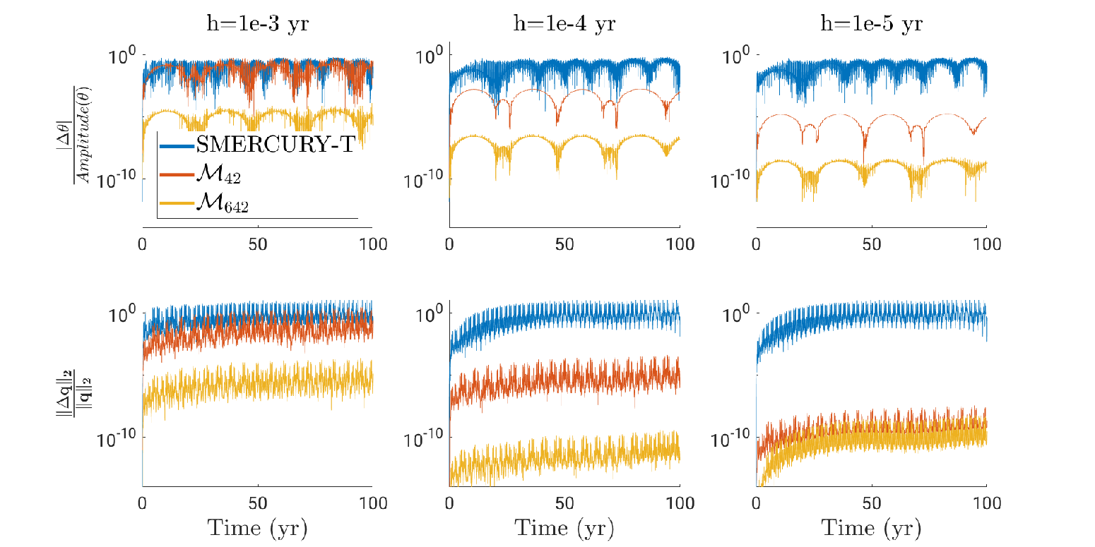
We now numerically illustrate how the integration error depends on $h$ for different numerical schemes, which include both methods we implemented in GRIT and SMERCURY-T. SMERCURY-T is a concurrent simulation package that can evolve an object’s spin-axis under obliquity tide (Kreyche et al. Submitted). It is based on the Mercury simulation package (Chambers 1999). Specifically, it includes a subroutine to evolve the spin-axis dynamics following the procedure outlined in (Lissauer et al. 2012), which is based on the Lie-Poisson integrator of rigid-body dynamics developed by Touma & Wisdom 1994. In addition, it includes a subroutine for obliquity tide following the algorithms outlined in Bolmont et al. 2015. The model for tidal interaction of SMERCURY-T is different from what we included in GRIT, which natually contains both obliquity tide and tidal effects due to non-tidally synchronized orbits. Thus, we focus on the rigid-body dynamics here, where we do not include tidal interactions in our convergence test. We also turned off, in comparisons presented here, our rigid-body rigid-body interaction option, which is mainly for accurate simulations of rigid bodies’ close encounters, because such interactions are supported only in GRIT.

We first test on the Sun-Earth-Moon system (fig. 5). One observation in this case is, if the step size is too large so that splitting into $H_{1}+H_{2}+H_{3}+H_{4}$ (GRIT’s $\mathcal{M}_{42}$, $\mathcal{M}_{642}$) doesn’t work, SMERCURY-T doesn’t work either (unlike expected by some). More precisely, with $h=2\cdot 10^{-2}$ yr, $\mathcal{M}_{42}$ and SMERCURY-T cannot resolve the the motion of the Moon orbiting around the Earth, whose period is a month, and even the performance of the 6th order method $\mathcal{M}_{642}$ is not ideal, and significant errors are observed in all methods. Accuracy is improved for stepsizes below this stability limit, and the rate of improvement is, as expected, dependent on the order of the numerical scheme. Consequently, higher order methods such as $\mathcal{M}_{42}$ and $\mathcal{M}_{642}$ show substantially smaller errors when smaller step sizes are applied (readers interested in understanding this together with computational costs are referred to Sec.IV.1.3).

We then test on a non-Keplerian system (note SMERCURY-T performs well for near Keplerian problems as designed): an Earth-like planet orbiting around two stars alternatively in a stellar binary system (fig. 6). As there is no single body that has the dominant mass of the system and the the planet is alternatively captured by the two stars, the planetary orbit is not nearly Keplerian, and splitting into $H_{1}+H_{2}+H_{3}+H_{4}$ is more accurate than SMERCURY-T for all choices of step sizes here. Specifically, as shown in fig. 6, the orbital position of SMERCURY-T saturates to $\mathcal{O}(1)$ relative error after a relatively short period of time, no matter if $h=10^{-3},10^{-4},\text{or }10^{-5}$ yr. The orbital inaccuracy naturally affects the spin angle as well. Meanwhile, $\mathcal{M}_{42}$ and $\mathcal{M}_{642}$ do not have this issue.

For reproducibility, the initial condition used is

References

- Agol et al. (2020) Agol, E. et al. 2020, arXiv e-prints, arXiv:2010.01074, 2010.01074
- Agol & Fabrycky (2018) Agol, E., & Fabrycky, D. C. 2018, Transit-Timing and Duration Variations for the Discovery and Characterization of Exoplanets, ed. H. J. Deeg & J. A. Belmonte
- Agol et al. (2021) Agol, E., Hernandez, D. M., & Langford, Z. 2021, arXiv e-prints, arXiv:2106.02188, 2106.02188
- Anderson et al. (1975) Anderson, J. D., Esposito, P. B., Martin, W., Thornton, C. L., & Muhleman, D. O. 1975, ApJ, 200, 221
- Benitez & Gallardo (2008) Benitez, F., & Gallardo, T. 2008, Celestial Mechanics and Dynamical Astronomy, 101, 289, 0709.1160
- Blanchet (2006) Blanchet, L. 2006, Living Reviews in Relativity, 9, 4
- Blanco-Cuaresma & Bolmont (2017) Blanco-Cuaresma, S., & Bolmont, E. 2017, in EWASS Special Session 4 (2017): Star-planet interactions (EWASS-SS4-2017), 1712.01281
- Blanes & Casas (2017) Blanes, S., & Casas, F. 2017, A concise introduction to geometric numerical integration (CRC press)
- Blanes et al. (2013) Blanes, S., Casas, F., Farres, A., Laskar, J., Makazaga, J., & Murua, A. 2013, Applied Numerical Mathematics, 68, 58
- Blanes et al. (2008) Blanes, S., Casas, F., & Murua, A. 2008, arXiv preprint arXiv:0812.0377
- Bolmont et al. (2020) Bolmont, E., Demory, B. O., Blanco-Cuaresma, S., Agol, E., Grimm, S. L., Auclair-Desrotour, P., Selsis, F., & Leleu, A. 2020, A&A, 635, A117, 2002.02015
- Bolmont et al. (2015) Bolmont, E., Raymond, S. N., Leconte, J., Hersant, F., & Correia, A. C. M. 2015, A&A, 583, A116, 1507.04751
- Bou-Rabee & Marsden (2009) Bou-Rabee, N., & Marsden, J. E. 2009, Foundations of Computational Mathematics, 9, 197
- Breiter et al. (2005) Breiter, S., Nesvorný, D., & Vokrouhlický, D. 2005, AJ, 130, 1267
- Celledoni et al. (2008) Celledoni, E., Fassò, F., Säfström, N., & Zanna, A. 2008, SIAM Journal on Scientific Computing, 30, 2084
- Celledoni et al. (2014) Celledoni, E., Marthinsen, H., & Owren, B. 2014, Journal of Computational Physics, 257, 1040
- Chambers (1999) Chambers, J. E. 1999, MNRAS, 304, 793
- Davis & Scheeres (2020) Davis, A. B., & Scheeres, D. J. 2020, The Planetary Science Journal, 1, 25
- Dullweber et al. (1997) Dullweber, A., Leimkuhler, B., & McLachlan, R. 1997, The Journal of chemical physics, 107, 5840
- Duncan et al. (1998) Duncan, M. J., Levison, H. F., & Lee, M. H. 1998, The Astronomical Journal, 116, 2067
- Eggleton et al. (1998) Eggleton, P. P., Kiseleva, L. G., & Hut, P. 1998, The Astrophysical Journal, 499, 853
- Eggleton & Kiseleva-Eggleton (2001) Eggleton, P. P., & Kiseleva-Eggleton, L. 2001, ApJ, 562, 1012, astro-ph/0104126
- Fabrycky & Tremaine (2007) Fabrycky, D., & Tremaine, S. 2007, ApJ, 669, 1298, 0705.4285
- Fahnestock & Scheeres (2008) Fahnestock, E. G., & Scheeres, D. J. 2008, Icarus, 194, 410
- Fassò (2003) Fassò, F. 2003, Journal of computational physics, 189, 527
- Giorgini et al. (1996) Giorgini, J. et al. 1996, in AAS/Division for Planetary Sciences Meeting Abstracts# 28, Vol. 28, 25–04
- Grimm et al. (2018) Grimm, S. L. et al. 2018, A&A, 613, A68, 1802.01377
- Hairer et al. (2006a) Hairer, E., Lubich, C., & Wanner, G. 2006a, Geometric Numerical Integration: Structure-Preserving Algorithms for Ordinary Differential Equations, 2nd edn. (Berlin Heidelberg New York: Springer)
- Hairer et al. (2006b) ——. 2006b, Geometric numerical integration: structure-preserving algorithms for ordinary differential equations, Vol. 31 (Springer Science & Business Media)
- Heyl & Gladman (2007) Heyl, J. S., & Gladman, B. J. 2007, MNRAS, 377, 1511, astro-ph/0610267
- Holm et al. (2009) Holm, D., Schmah, T., & Stoica, C. 2009, Geometric mechanics and symmetry: from finite to infinite dimensions, Oxford texts in applied and engineering mathematics (Oxford University Press)
- Hou et al. (2017) Hou, X., Scheeres, D. J., & Xin, X. 2017, Celestial Mechanics and Dynamical Astronomy, 127, 369
- Hut (1981) Hut, P. 1981, A&A, 99, 126
- Iserles et al. (2000) Iserles, A., Munthe-Kaas, H. Z., Nørsett, S. P., & Zanna, A. 2000, Acta numerica, 9, 215
- Joshi et al. (1997) Joshi, M. M., Haberle, R. M., & Reynolds, R. T. 1997, Icarus, 129, 450
- Kasting et al. (1993) Kasting, J. F., Whitmire, D. P., & Reynolds, R. T. 1993, Icarus, 101, 108
- Kreyche et al. (Submitted) Kreyche, S., Barnes, J., Quarles, B., & Chambers, J. Submitted, Planetary Science Journal
- Laskar et al. (1993) Laskar, J., Joutel, F., & Robutel, P. 1993, Nature, 361, 615
- Laskar & Robutel (1993) Laskar, J., & Robutel, P. 1993, Nature, 361, 608
- Laskar & Robutel (2001) Laskar, J., & Robutel, P. 2001, Celestial Mechanics and Dynamical Astronomy, 80, 39
- Lee et al. (2007) Lee, T., Leok, M., & McClamroch, N. H. 2007, Celestial Mechanics and Dynamical Astronomy, 98, 121
- Lee et al. (2005) Lee, T., McClamroch, N. H., & Leok, M. 2005, in Proceedings of 2005 IEEE Conference on Control Applications, 2005. CCA 2005., IEEE, 962–967
- Leimkuhler & Reich (2004) Leimkuhler, B., & Reich, S. 2004, Cambridge Monographs on Applied and Computational Mathematics, Vol. 14, Simulating Hamiltonian dynamics (Cambridge: Cambridge University Press), xvi+379
- Li & Batygin (2014) Li, G., & Batygin, K. 2014, The Astrophysical Journal, 790, 69
- Li et al. (2021) Li, J., Lai, D., Anderson, K. R., & Pu, B. 2021, MNRAS, 501, 1621, 2006.10067
- Lissauer et al. (2012) Lissauer, J. J., Barnes, J. W., & Chambers, J. E. 2012, Icarus, 217, 77
- Maciejewski et al. (2018) Maciejewski, G. et al. 2018, ACTA ASTRONOMICA, 68, 371, 1812.02438
- Mardling & Lin (2002) Mardling, R. A., & Lin, D. N. C. 2002, ApJ, 573, 829
- Marsden & Ratiu (1994) Marsden, J. E., & Ratiu, T. S. 1994, Introduction to mechanics and symmetry: a basic exposition of classical mechanical systems (Springer)
- McLachlan (1995) McLachlan, R. I. 1995, BIT numerical mathematics, 35, 258
- McLachlan & Quispel (2002) McLachlan, R. I., & Quispel, G. R. W. 2002, Acta Numerica, 11, 341
- Meyer & Scheeres (2021) Meyer, A. J., & Scheeres, D. J. 2021, Icarus, 367, 114554
- Millholland & Laughlin (2019) Millholland, S., & Laughlin, G. 2019, Nature Astronomy, 3, 424, 1903.01386
- Miralda-Escudé (2002) Miralda-Escudé, J. 2002, ApJ, 564, 1019, astro-ph/0104034
- Muirhead et al. (2015) Muirhead, P. S. et al. 2015, ApJ, 801, 18, 1501.01305
- Ragozzine & Wolf (2009) Ragozzine, D., & Wolf, A. S. 2009, ApJ, 698, 1778, 0807.2856
- Reich & Zentrum (1996) Reich, S., & Zentrum, K.-Z. 1996, Fields Inst. Commun, 10, 181
- Sanz-Serna & Calvo (1994) Sanz-Serna, J., & Calvo, M. 1994, Numerical Hamiltonian problems, 1st edn. (Chapman and Hall/CRC)
- Suzuki (1990) Suzuki, M. 1990, Physics Letters A, 146, 319
- Tamayo et al. (2017) Tamayo, D., Rein, H., Petrovich, C., & Murray, N. 2017, ApJ, 840, L19, 1704.02957
- Tamayo et al. (2020) Tamayo, D., Rein, H., Shi, P., & Hernandez, D. M. 2020, MNRAS, 491, 2885, 1908.05634
- Tao & Ohsawa (2020) Tao, M., & Ohsawa, T. 2020, in International Conference on Artificial Intelligence and Statistics, PMLR, 4269–4280
- Tao et al. (2010) Tao, M., Owhadi, H., & Marsden, J. E. 2010, Multiscale Modeling & Simulation, 8, 1269
- Touma & Wisdom (1994) Touma, J., & Wisdom, J. 1994, AJ, 107, 1189
- Van Hoolst et al. (2008) Van Hoolst, T., Rambaux, N., Karatekin, Ö., Dehant, V., & Rivoldini, A. 2008, Icarus, 195, 386
- van Zon & Schofield (2007) van Zon, R., & Schofield, J. 2007, Physical Review E, 75, 056701
- Vilmart (2008) Vilmart, G. 2008, Journal of computational physics, 227, 7083
- Vinson et al. (2019) Vinson, A. M., Tamayo, D., & Hansen, B. M. S. 2019, MNRAS, 488, 5739, 1905.11419
- Wisdom & Holman (1991) Wisdom, J., & Holman, M. 1991, The Astronomical Journal, 102, 1528
- Wordsworth (2015) Wordsworth, R. 2015, ApJ, 806, 180, 1412.5575
- Yoshida (1990) Yoshida, H. 1990, Physics letters A, 150, 262
- Zhu et al. (2018) Zhu, W., Petrovich, C., Wu, Y., Dong, S., & Xie, J. 2018, ApJ, 860, 101, 1802.09526
Appendix A Approximation of the Potential Energy
The procedure to approximate in eq. 9 by Taylor expansion is shown below: