An analytical study of flatness and intermittency through Riemann’s non-differentiable functions

Let us adapt the concepts presented in the introduction to the setting of functions, following Jaffard [22, 23, 24]. Let $\mathbb{T}=\mathbb{R}/\mathbb{Z}$ be the torus, $a_{n}\in\mathbb{C}$ and $f:\mathbb{T}\to\mathbb{C}$ a periodic function with Fourier series $f(x)=\sum_{n\in\mathbb{Z}}{a_{n}\,e^{2\pi inx}}$. The usual way [23, p. 946] to adapt structure functions from (2) to $f$ is

and high-pass filters from (8) as

To avoid $f_{\geq N}\equiv 0$, we assume that $f$ has infinitely many nonzero $a_{n}$ coefficients. Low-pass filters are defined analogously by $f_{\leq N}(x)=\sum_{|n|\leq N}{a_{n}e^{2\pi inx}}$.

In the same way that the deviation of $S_{4}(\ell)$ from Kolmogorov’s theory is measured by the flatness (7), the generalized flatness

is the analogue measure corresponding to $S_{p}(\ell)$, see [18, (8.6)]. Moreover, the generalized kurtosis on the right hand-side is an alternative measure of the thickness of the tails of a probability distribution. Thus, we adapt the flatness from (7) and (8) as follows.

In [3], filaments, we proved that

where $R_{1}$ is Riemann’s non-differentiable function. Here we study the generalizations $R_{s}$ defined in (10) to compare the two flatness $F_{f,p}(N)$ and $G_{f,p}(\ell)$ in a more general situation. These functions are absolutely convergent when $s>1/2$, but can be shown to be in $L^{p}(\mathbb{T})$ for lower values of $s$, so for $p\geq 2$ we define the threshold

Theorem A follows from the behavior of $\lVert(R_{s})_{\geq N}\rVert_{L^{p}(\mathbb{T})}$, which we compute in Theorem 5.1. In the same way, Theorem B is a consequence of the behavior of the structure functions $S_{p}(\ell)$, which we give in Theorem 6.1. Both Theorems 5.1 and 6.1 are a consequence of estimates for the Littlewood-Paley blocks and low-pass filters of $R_{s}$ that we compute in Proposition 4.2 and in Theorem 4.4, respectively. They could be of independent interest; for instance, they are related to Rudin’s $\Lambda(p)$-set problem for the set of squares [25, 4], which is relevant among others in the study of the nonlinear Schrödinger equation [5].

We also prove the multifractal formalism for the functions $R_{s}$. Let us briefly discuss how (11) is adapted to the setting of functions; for a detailed account we refer the reader to [23, 24]. A function $f$ is said to be $\alpha$-Hölder at the point $x_{0}$, and written $f\in C^{\alpha}(x_{0})$, if there is a polynomial $P$ of degree at most $\alpha$ such that $\left|f(x_{0}+h)-P(h)\right|\leq C\,h^{\alpha}$, and the Hölder exponent of $f$ at $x_{0}$ is $\alpha_{f}(x_{0})=\sup\{\alpha\mid f\in C^{\alpha}(x_{0})\}$. The $\alpha$-Hölder regularity sets are $D_{\alpha}=\{x\mid\alpha_{f}(x)=\alpha\}$, and $d(\alpha)=\dim_{\mathcal{H}}D_{\alpha}$ is the Hausdorff dimension of these sets, called the spectrum of singularities of $f$. On the other hand, the exponent $\zeta_{p}$ can be defined in several ways [23] which we discuss later in (26).

In [22, Corollary 2], Jaffard proved that

where by convention the dimension is $-\infty$ when the set is empty. Thus, in order to prove Theorem D, we compute $\eta_{s}(p)$:

The proof of Proposition E is directly linked to the proof of Theorem A, since $\eta_{s}(p)$ is related to the Littlewood-Paley decomposition of $R_{s}$ and, thus, to the $L^{p}$ estimates of the high-pass filters $\lVert(R_{s})_{\geq N}\rVert_{L^{p}(\mathbb{T})}$ which we compute in Theorem 5.1.

Theorems A and B show that the two flatnesses $F_{s,p}$ and $G_{s,p}$ do not always coincide. A visual representation of this discrepancy is shown in Figure 1. While the flatness of high-pass filters (Figure 1(a)) does not depend on $s$, structure functions produce a handful of regions (Figure 1(b)).

Up to the behavior in the boundaries, these regions are:

• •

  Region . The non-intermittent region, where the flatness is constant. The regions coincide only when $p<4$.

• •

  Region . We have intermittent, divergent power laws $F_{R_{s},p}(N)\simeq N^{p/4-1}$ and $G_{R_{s},p}(\ell)\simeq\ell^{-(p/4-1)}$. The regions match when $p>4$ and $s<5/4$.

• •

  Region . Exclusive of structure functions, where $G_{R_{s},p}(\ell)\simeq\ell^{-(3p/2-1-ps)}$. For fixed $p$, intermittency is weaker than in region , since

  $$\ell^{-(3p/2-1-ps)}\ll\ell^{-(p/4-1)}\qquad\text{ when }s>5/4.$$

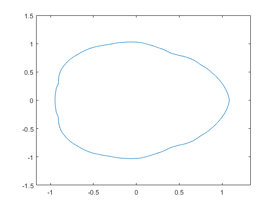
As we said in the introduction, these coincidences and discrepancies have also been observed in experimental turbulence [6, 11]. Indeed, we can establish an analogy between our results for $R_{s}$ in Theorems A and B and the effect of viscosity in a turbulent flow, where the parameter $s$ plays the role of viscosity. For that, in Figure 2 we plot the complex functions $R_{s}$ (10) on the left column and the classical real-valued $\operatorname{Im}R_{s}$ on the right column. Different $s$ produce quite different situations, larger $s$ showing less oscillations and more regularity. When $s<5/4$, Figures 2(b) and 2(d) are similar to the typical irregular velocity profile of turbulent flows in the inertial range, where the effect of viscosity is small. When $s\in(5/4,3/2)$, Figure 2(f) is smoother, representing a transition to the dissipation range where viscosity starts having an effect; we further discuss this range in the end of the section. Finally, when $s>3/2$, Figure 2(h) represents the dissipation range where viscosity dominates and completely smooths out the velocity. Thus, the two flatnesses coincide only for $s$ corresponding to the inertial range, so this analogy suggests that in experimental observations the two approaches should be interchangeable in the inertial range, but not in the dissipation range.

This analogy can be further supported analytically. The main difference between the inertial and the dissipation range is that the flow is extremely irregular in the former, but smooth in the latter. The same goes for $R_{s}$, since Jaffard’s result in (24) implies that it is almost nowhere differentiable when $s<5/4$, but almost everywhere differentiable when $5/4<s<3/2$ and everywhere differentiable when $s\geq 3/2$. Thus, flatnesses coincide only in the irregular inertial range, when $R_{s}$ is almost nowhere differentiable. Up to lower order corrections, this is a general fact that is connected to the exponent $\zeta_{p}$ in the multifractal formalism (11). According to [23, Proposition 3.1], $\zeta_{p}$ may be equivalently defined in terms of several Sobolev-like spaces, such as

where $B^{\sigma}_{p,q}$ are Besov spaces, $H^{\sigma,p}$ are Nikolskii spaces, $L^{\sigma,p}$ are Bessel potential spaces and $W^{\sigma,p}$ are Sobolev-Slobodeckij spaces. The first two are directly connected to Fourier filters and structure functions respectively, as we explain in the following lines.

Besov spaces in $\mathbb{T}$ are based in the Littlewood-Paley decomposition of a function,

since $f\in B^{\sigma}_{p,q}$ if the sequence $\left(2^{k\sigma}\lVert P_{k}f\rVert_{p}\right)_{k}$ is in $\ell^{q}$. That means that

Denoting $N=2^{k}$, we see that $P_{k}f=f_{\simeq N}$ is a band-pass filter of $f$. From (27) and the definition of $\zeta_{p}$ in (26), formally we have $\lVert f_{\simeq N}\rVert_{p}^{p}\simeq N^{-\zeta_{p}}$, where lower order corrections like logarithms are not accounted for. Also, in many situations like for $R_{s}$, $\lVert f_{\simeq N}\rVert_{p}\simeq\lVert f_{\geq N}\rVert_{p}$ holds.

Regarding Nikolskii spaces $H^{\sigma,p}$, the original purpose of $\zeta_{p}$ as the power law of structure functions (12) is recovered. Indeed, if $\sigma=m+\sigma^{\prime}$ with $m\in\mathbb{N}$ and $\sigma^{\prime}\in[0,1)$,

where $D^{m}f$ is the $m$-th derivative of $f$. When $\sigma<1$, there is a clear connection with $S_{f,p}(\ell)$, since if $\zeta_{p}<p$ the definition of $\zeta_{p}$ (26) formally implies $S_{f,p}(\ell)\simeq\ell^{\zeta_{p}}$.

Consequently, joining these two interpretations of $\zeta_{p}$, structure functions and band-pass filters follow the same power law up to lower order corrections if $\zeta_{p}<p$ (roughly, one may think of this situation as $f^{\prime}\notin L^{p}$). Thus, when $f$ is not regular enough, like the velocity of the flow in the inertial range, one should in general expect that $F_{f,p}$ and $G_{f,p}$ have a similar behavior. On the other hand, when the function is regular enough so that $\zeta_{p}>p$, the Besov space characterization still gives $\lVert f_{\simeq N}\rVert_{p}^{p}\simeq N^{-\zeta_{p}}$, but for the structure functions we may formally write

if $N^{-1}\simeq\ell$. The reason behind this is that, according to the definition $H^{\sigma,p}$ in (29), $\zeta_{p}$ describes no longer the structure functions of $f$ but of its derivatives. Thus, we should expect the two flatnesses to coincide in irregular situations like in the inertial range of turbulence, but not when the element under consideration becomes regular, like in the dissipation range by the effect of viscosity.

We may as well draw an interesting analogy with the debate on the correctness of the multifractal formalism (11) in the dissipation range. Indeed, according to Theorem D, the function $R_{s}$ satisfies the multifractal formalism with the exponent $\zeta_{p}$ defined as in (26), that is, with the exponent corresponding to high-pass filters. But what about the exponent $\xi_{p}$ coming from the structure functions $S_{p}(\ell)\simeq\ell^{\xi_{p}}$, as proposed in the original multifractal formalism?

As we prove in Theorems B and 6.1, we have $\xi_{p}=\zeta_{p}$ for $s<5/4$, in which case the multifractal formalism is satisfied also with structure functions. However, when $s\geq 5/4$ the exponents $\xi_{p}$ and $\zeta_{p}$ are no longer equal, and since by Theorem D the multifractal formalism still holds with $\zeta_{p}$, it can not be satisfied with $\xi_{p}$ from structure functions. We can, though, separate two regimes:

• •

  if $s>3/2$, then $R_{s}$ is differentiable, so from the point of view of turbulence there is not much left to understand in terms of irregularity. As suggested before, this is analog to the small scales where viscosity clearly dominates and the velocity of the fluid becomes smooth. In analytic terms, even if the structure functions of $R_{s}$ do not satisfy the multifractal formalism, it is in fact hidden in the derivatives of $R_{s}$. Indeed, since $s-1>1/2$, then $R_{s}^{\prime}=R_{s-1}$ is absolutely convergent and belongs to all $L^{p}$ spaces. Thus, if $3/2<s<5/2$, by (29) $\zeta_{p}$ captures the behavior of the structure functions of $R^{\prime}_{s}$. In other words, it is the structure functions of $R_{s}^{\prime}$ which satisfy the multifractal formalism. For $s>5/2$, the same works with higher order derivatives.

• •

  But if $5/4<s<3/2$, $R_{s}^{\prime}=R_{s-1}$ is not absolutely convergent, it is not in all $L^{p}$ and $\xi_{p}$ is not defined for all $p$. In other words, there is no evident way to relate $\zeta_{p}$ with structure functions, so there is no direct way to justify the multifractal formalism from the approach of structure functions.

  In turbulence, this is analog to the idea that the dissipation scale is not a single scale, but rather a whole range of scales of transition from the inertial range to the dissipative range, where the multifractal formalism may not be accurate enough. Corrections to the multifractal formalism in this dissipative transtion have been proposed in the physical literature (see the review in [18, Chapter 8.5.5.]) It would be a very interesting task to further study this transition regime from a rigorous mathematical perspective.

We briefly describe the structure of this article.

• •

  In Section 3 we prove technical lemmas that we use throughout the paper.

• •

  In Section 4 we give $L^{p}$ estimates on the Littlewood-Paley blocks (Proposition 4.2) and low-pass filters (Theorem 4.4) of $R_{s}$. We use them to prove the results in Sections 5 and 6, but as mentioned, they could also be of independent interest.

• •

  In Section 5 - Theorem 5.1, we compute the behavior of the high-pass filters $\lVert(R_{s})_{\geq N}\rVert_{p}$. For that, we use the Littlewood-Paley decomposition and Proposition 4.2. Theorem A is a direct consequence of it.

• •

  In Section 6 - Theorem 6.1, we compute the behavior of the structure functions $S_{R_{s},p}(\ell)$ using the low pass filters in Theorem 4.4. Theorem B immediately follows.

• •

  In Section 7 we prove Theorem D and Proposition E concerning the multifractal formalism for $R_{s}$.

Throughout the paper, we adopt the following notation.

For inequalities:

• •

  We write $A\lesssim B$ when there is a constant $C>0$, independent of the parameters of the problem, such that $A\leq CB$. We write $A\simeq B$ when $A\lesssim B$ and $B\lesssim A$. The implicit constants in the former inequalities may change from line to line. If the constants of the former inequalities depend on a certain parameter, say $p$, then we write $\lesssim_{p}$ and $\simeq_{p}$.

For the limits of a sum:

• •

  If either of $A,B\in\mathbb{R}$ are not integers, we denote $\sum_{n=A}^{B}=\sum_{n\in[A,B]\cap\mathbb{Z}}$.

For $L^{p}$ norms and the exponential functions:

• •

  We write $\lVert\cdot\rVert_{p}$ instead of $\lVert\cdot\rVert_{L^{p}(\mathbb{T})}$.

• •

  We denote $e_{n}(x)=e^{2\pi inx}$.

• •

  Many times, especially after Section 4, we will write $\left\lVert\sum_{n=A}^{B}e^{2\pi in^{2}x}/n^{2s}\right\rVert_{p}$ instead of $\left\lVert\sum_{n=A}^{B}e_{n^{2}}/n^{2s}\right\rVert_{p}$.

For the Fourier transform:

• •

  We denote the Fourier transform $\mathcal{F}(f)$ by $\widehat{f}$ and the inverse Fourier transform $\mathcal{F}^{-1}(f)$ by $f^{\vee}$.

  (31)

  $$\widehat{f}(\xi)=\int_{\mathbb{R}}f(x)\,e^{-2\pi i\xi x}\,\mathrm{d}x,\qquad\qquad f^{\vee}(\xi)=\int_{\mathbb{R}}f(x)\,e^{2\pi i\xi x}\,\mathrm{d}x.$$

References

• [1] Banica, V., and Vega, L. Riemann’s non-differentiable function and the binormal curvature flow. Preprint, arXiv: 2007.07184 (2020).
• [2] Barral, J., and Seuret, S. Besov spaces in multifractal environment and the Frisch-Parisi conjecture. Preprint, arXiv: 2007.00971 (2020).
• [3] Boritchev, A., Eceizabarrena, D., and Da Rocha, V. V. Intermittency of Riemann’s non-differentiable function through the fourth-order flatness. J. Math. Phys. 62, 9 (2021), Paper No. 093101, 14.
• [4] Bourgain, J. On Λ⁡(p)\Lambda(p)-subsets of squares. Israel J. Math. 67, 3 (1989), 291–311.
• [5] Bourgain, J. Fourier transform restriction phenomena for certain lattice subsets and applications to nonlinear evolution equations. I. Schrödinger equations. Geom. Funct. Anal. 3, 2 (1993), 107–156.
• [6] Brun, C., and Pumir, A. Statistics of Fourier modes in a turbulent flow. Phys. Rev. E 63 (2001), 056313.
• [7] Chamizo, F., and Córdoba, A. Differentiability and dimension of some fractal Fourier series. Adv. Math. 142, 2 (1999), 335–354.
• [8] Chamizo, F., and Ubis, A. Some Fourier series with gaps. J. Anal. Math. 101 (2007), 179–197.
• [9] Chamizo, F., and Ubis, A. Multifractal behavior of polynomial Fourier series. Adv. Math. 250 (2014), 1–34.
• [10] Chevillard, L., Castaing, B., Arneodo, A., Lévêque, E., Pinton, J.-F., and Roux, S. G. A phenomenological theory of Eulerian and Lagrangian velocity fluctuations in turbulent flows. C. R. Phys. 13 (2012), 899–928.
• [11] Chevillard, L., Mazellier, N., Poulain, C., Gagne, Y., and Baudet, C. Statistics of Fourier modes of velocity and vorticity in turbulent flows: intermittency and long-range correlations. Phys. Rev. Lett. 95 (2005), 200203.
• [12] Daubechies, I., and Lagarias, J. C. On the thermodynamic formalism for multifractal functions. vol. 6. 1994, pp. 1033–1070. Special issue dedicated to Elliott H. Lieb.
• [13] de la Hoz, F., and Vega, L. Vortex filament equation for a regular polygon. Nonlinearity 27, 12 (2014), 3031–3057.
• [14] Eceizabarrena, D. Some geometric properties of Riemann’s non-differentiable function. C. R. Math. Acad. Sci. Paris 357, 11-12 (2019), 846–850.
• [15] Eceizabarrena, D. Geometric differentiability of Riemann’s non-differentiable function. Adv. Math. 366 (2020), 107091, 39.
• [16] Eceizabarrena, D. On the Hausdorff dimension of Riemann’s non-differentiable function. Trans. Amer. Math. Soc. 374, 11 (2021), 7679–7713.
• [17] Eyink, G. L. Besov spaces and the multifractal hypothesis. vol. 78. 1995, pp. 353–375. Papers dedicated to the memory of Lars Onsager.
• [18] Frisch, U. Turbulence. Cambridge University Press, Cambridge, 1995. The legacy of A. N. Kolmogorov.
• [19] Frisch, U., and Parisi, G. On the singularity structure of fully developed turbulence. In Proc. Int. Summer School Phys. Enrico Fermi (1985), pp. 84–88. Appendix to ‘Fully developed turbulence and intermittency’, by U. Frisch.
• [20] Grafakos, L. Classical Fourier analysis, second ed., vol. 249 of Graduate Texts in Mathematics. Springer, 2008.
• [21] Jaffard, S. Sur la dimension de Hausdorff des points singuliers d’une fonction. C. R. Acad. Sci. Paris Sér. I Math. 314, 1 (1992), 31–36.
• [22] Jaffard, S. The spectrum of singularities of Riemann’s function. Rev. Mat. Iberoamericana 12, 2 (1996), 441–460.
• [23] Jaffard, S. Multifractal formalism for functions. I. Results valid for all functions. SIAM J. Math. Anal. 28, 4 (1997), 944–970.
• [24] Jaffard, S. Multifractal formalism for functions. II. Self-similar functions. SIAM J. Math. Anal. 28, 4 (1997), 971–998.
• [25] Rudin, W. Trigonometric series with gaps. J. Math. Mech. 9 (1960), 203–227.
• [26] Westfall, P. H. Kurtosis as peakedness, 1905–2014. r.i.p. Amer. Statist. 68, 3 (2014), 191–195.
• [27] Zalcwasser, Z. Sur les polynomes associés aux fonctions modulaires θ\theta. Studia Math. 7 (1938), 16–35.