Heat Blanketing Envelopes of Neutron StarsJournal: Physics Reports
Abstract
Near the surface of any neutron star there is a thin heat blanketing envelope that produces substantial thermal insulation of warm neutron star interiors and that relates the internal temperature of the star to its effective surface temperature. Physical processes in the blanketing envelopes are reasonably clear but the chemical composition is not. The latter circumstance complicates inferring physical parameters of matter in the stellar interiors from observations of the thermal surface radiation of the stars and urges one to elaborate the models of blanketing envelopes. We outline physical properties of these envelopes, particularly, the equation of state, thermal conduction, ion diffusion and others. Various models of heat blankets are reviewed, such as composed of separate layers of different elements, or containing diffusive binary ion mixtures in or out of diffusion equilibrium. The effects of strong magnetic fields in the envelopes are outlined as well as the effects of high temperatures which induce strong neutrino emission in the envelopes themselves. Finally, we discuss how the properties of the heat blankets affect thermal evolution of neutron stars and the ability to infer important information on internal structure of neutron stars from observations.
Keywords:
Neutron stars , Diffusion , Cooling1 Introduction: Neutron stars, their superdense matter and thermal insulation
Neutron stars (e.g., Shapiro and Teukolsky 1983; Haensel et al. 2007) are the most compact stellar objects, with typical masses , where is the solar mass, and radii km. Their mean mass density is a few , where g cm-3 is the density of standard saturated nuclear matter. The central density of massive neutron stars exceeds by about one order of magnitude. Neutron stars are born in supernova explosions and demonstrate a wealth of manifestations observed by the methods of multiwavelength astronomy (from radio to gamma rays) and by gravitational observatories; they are also expected to be observed by neutrino observatories.
According to current theories (e.g., Haensel et al. 2007), a neutron star can roughly be divided into a relatively light and thin crust (about 1% by mass and 10% by radius) and a massive and bulky core. The core is thought to be liquid; it contains strongly degenerate nucleons, electrons, muons, and (possibly) other particles like hyperons and/or deconfined quarks, which are distributed uniformly on the microscopic scale. In contrast, the crust contains aggregates of nucleons of microscopic scale (nuclei). The “crust” in the broad sense consists of liquid “ocean”, solid layers (the crust in the proper sense), and possibly layers of non-spherical nuclei that behave like liquid crystals (so called “pasta phases”, which constitute a “mantle” of the star). The crust is divided into the “outer crust”, where the nuclei are immersed in the fluid of electrons, and the “inner crust”, which additionally contains the fluid of free neutrons (and possibly free protons in the deepest layers).
Since the core contains superdense matter, it is the most mysterious and interesting part of neutron stars; the composition, equation of state and many other properties of this matter are poorly known. Their study is of fundamental importance for astrophysics and other branches of physics including nuclear physics, physics of elementary particles, and condensed matter physics. The basic problems are that (i) it is difficult to explore the superdense matter in terrestrial laboratories; (ii) its properties cannot be calculated reliably because of the absence of practical theory for describing strong interactions of baryons with account of many-body effects. Some properties of superdense matter can be studied in collider experiments on heavy ions collisions, on neutron skin measurements and in some other ways (e.g., Lattimer and Prakash 2016; Mondal et al. 2016; Oertel et al. 2017), but these data are incomplete. Very dense matter (), which can appear after the deconfinement of quarks, can be analyzed by the methods of perturbative quantum chromodynamics (e.g., Haensel et al. 2007; Machleidt and Entem 2011). However, the matter of the most interesting, intermediate density, , cannot be accurately studied in laboratory experiment and theory but it can be investigated using observations of neutron stars.
The outer crust extends from the stellar surface to the neutron drip density g cm-3; its mass is . The inner crust extends from to the crust/core interface at g cm-3. The electrons are mainly degenerate except for the very surface layer. At densities g cm-3 they are non-relativistic; at higher they become relativistic, and the atomic nuclei become progressively more neutron-rich. The free neutrons and the nucleons within the nuclei can be in superfluid state.
The astrophysical methods to explore the nature of superdense matter in neutron stars are complex. Generally, they consist of modeling various processes accessible in observations of neutron stars. Then one can compare theoretical models with observations and select those models which are most suitable. In particular, one can model thermal evolution of neutron stars with different microphysics of matter and confront such models with the measurements of surface temperatures and ages of neutron stars (as reviewed by Yakovlev and Pethick 2004; Page 2009; Tsuruta 2009; Potekhin et al. 2015b; Geppert 2017). This method has been used for many decades and faces many difficulties. We will focus on one important obstacle associated with our poor knowledge of chemical composition of heat blanketing envelopes of neutron stars.
A heat blanketing (thermally insulating) envelope is situated under the stellar atmosphere and is thin; its mass is . The surface temperature of the star (), that can be measured, is typically much smaller than the internal temperature (). The relation between and is a complex problem, because the composition of the heat blankets is often unknown. By varying the composition one can obtain different temperatures at a fixed temperature , with different conclusions on properties of superdense matter. In addition, the composition of the heat blanket may vary in time owing to accretion, diffusion and nuclear burning. These effects are not easy to study, particularly, because the plasma of ions can be strongly non-ideal.
Therefore, to explore properties of superdense matter inside neutron stars one needs a reliable theory of heat blanketing envelopes. While the main features of superdense matter are still basically unclear, the properties of heat blankets are based on a much more elaborated physics of not very dense plasma. However, the problem of heat blankets creates a really serious obstacle to investigate the superdense matter. Our aim is to describe the current status of the problem.
In Section 2 we outline the basic equations of neutron star structure and evolution. Section 3 describes the main properties of the heat blankets. In Section 4 we consider a simple semi-analytic model by Ventura and Potekhin 2001 of a non-magnetic heat blanket which explains its main features without detailed numerical computations. Then we discuss (Section 5) the properties of non-magnetic blanketing envelopes constructed by Potekhin et al. 1997; they consist either of iron, or of the layers of lighter elements (hydrogen, helium, carbon) and possibly the layer of iron at the bottom. Section 6 is focused on diffusion of ions in the surface layers of neutron stars. In Section 7 we describe diffusive blanketing envelopes of non-magnetic neutron stars; these envelopes have been computed for binary ionic mixtures (H-He, He-C, C-Fe). The next Section 8 is devoted to the envelopes of magnetized stars. Unlike the non-magnetic envelopes, where the temperature distribution is isotropic (spherically symmetric), the temperature distribution in this case can be highly anisotropic in response to anisotropic character of heat transport in a magnetic field. In the end of this section we outline also other models of heat blankets – for hot stars and magnetars (where the neutrino emission can be important in the blanket itself); for accreting neutron stars, where nuclear burning in the blanket can be significant; and for some other cases. In Sections 9 and 10 we present some illustrative examples how the blankets may affect neutron star evolution. Finally, we conclude in Section 11. Some aspects of the heat-blanket theory are applicable also for white dwarfs. In Appendix A and Appendix B we present, respectively, analytic fitting formulas for the diffusion coefficient in a binary ion mixture and for the relations between the surface and internal temperatures for binary heat-blanketing envelopes.
2 Equations of neutron star structure and thermal evolution
Let us present general equations of neutron star structure and thermal evolution. To shorten this introductory task we will restrict ourselves to spherically symmetric stars with spherically symmetric temperature distribution inside them, neglecting the effects of magnetic fields and rotation. The effects of strong magnetic fields will be briefly discussed in Section 8.
2.1 Hydrostatic equilibrium
Neutron stars are relativistic objects and should be studied using General Relativity. The importance of relativistic effects is characterized by the parameter , where is the stellar radius, is the gravitational radius, and the gravitational constant. Typically, 0.2 – 0.4 for neutron stars, and for all other stars.
The metric within or around a stationary and spherically symmetric star is (e.g., Haensel et al. 2007)
| (2.1) |
where is a time-like coordinate (Schwarzschild time for a distant observer), is a radial coordinate, and are the polar angle and azimuth, respectively, while and are two metric functions of . The angular geometry (with respect to and ) is the same as in flat space-time because of spherical symmetry, but space-time is generally curved along and “directions.” In flat space-time, we would have .
It is well known that in Eq. (2.1) is the circumferential radius which determines proper length of the circle, ; proper area of a spherical surface at given is . The proper radial length from the stellar center, , is generally different from . Hence determines curvature in the radial direction. It is related to the gravitational mass contained inside a sphere with radial coordinate ,
| (2.2) |
The gravitational mass is smaller than the baryon mass (“rest mass”) due to gravitational mass defect.
A proper radial length element and a proper volume between close spherical shells are
| (2.3) |
A proper time interval in a local rest-frame is
| (2.4) |
Therefore, determines gravitational dilatation of time and gravitational redshift of signals. If a local source produces a periodic signal of frequency at , a distant observer (, ) will detect a signal of frequency .
The equations of hydrostatic structure of the star follow directly from Einstein equations,
| (2.5) | |||||
| (2.6) | |||||
| (2.7) |
where is the pressure and is the energy density of the stellar matter. The quantity , introduced instead of , is called the mass density of the matter. It includes baryon mass density and mass defects produced by microscopic particle motion, by strong, weak and electromagnetic interactions, but not by the gravitational interaction. The mass density in dense neutron star cores is noticeably different from the traditional baryon mass density.
Equation (2.5) is the Tolman-Oppenheimer-Volkoff equation of hydrostatic equilibrium (Tolman 1939; Oppenheimer and Volkoff 1939), Equation (2.6) describes mass balance, while Eq. (2.7) is a relativistic version of the equation for the dimensionless gravitational potential . These equations should be supplemented by the equation of state (EoS) that relates pressure to density and temperature, . In the layers where free leptons or nucleons are strongly degenerate, the EoS is almost independent of temperature. Then in the above equations one can use a barotropic EoS, that is . Recalling that a neutron star is composed mostly of strongly degenerate matter, we can conclude that the neutron star structure is largely independent of its thermal state. Temperature effects on hydrostatic structure are important only near the surface (in the atmosphere and the heat blanketing envelope).
Equation (2.5) can be rewritten in the Newtonian form
| (2.8) |
where
| (2.9) |
is a local gravitational acceleration.
Outside the star one has and , so that is constant, which is the total gravitational mass of the star. In this case, meaning the Schwarzschild metric outside the star, with being the Schwarzschild radius. At , the Schwarzschild space-time becomes asymptotically flat. Finally, for a non-relativistic star (, , ) Eqs. (2.5)–(2.7) reduce to the Newtonian equations of stellar equilibrium, where plays role of the Newtonian gravitational potential.
2.2 Thermal structure and evolution
The thermal structure of a neutron star is characterized by the internal distribution of local temperature . In contrast to the hydrostatic structure that undergoes almost no evolution, the thermal structure may strongly evolve and affect observational manifestations of neutron stars. Let us consider not too hot (and not too young) stars, with internal temperatures K (of age min); they are fully transparent for neutrinos (e.g., Pons et al. 1999).
Generally, the thermal evolution is governed by heat conduction within the star, with subsequent thermal emission from the surface, and also by neutrino cooling from the bulk of the star and possibly by some reheating from inside or from the surface.
General relativistic equations of thermal evolution of a spherically symmetric star were derived by Thorne 1966; Thorne 1977. Basically, one needs to solve the two equations, of thermal balance and thermal transport.
The thermal balance equation can be written as (Richardson et al. 1982),
| (2.10) |
where is the neutrino cooling rate per unit volume, is the heating power per unit volume (if any), is the entropy per unit volume, and is the “local luminosity” (non-neutrino energy transported through a sphere of radial coordinate per unit time); all these quantities depend on and . The thermal flux density associated with is . It may be convenient to include the entropy changes related to structural modifications (such as phase transitions) into . Then , where is the heat capacity per unit volume at constant pressure. The heat capacities at constant volume and constant pressure are almost equal in the strongly degenerate matter, that is almost everywhere throughout the star (e.g., Haensel et al. 2007); therefore we will not distinguish between them. The quantities , , and have to be determined from microscopic thermodynamic and kinetic theories and from a model of internal heating (if available). In the absence of the latter (), one deals with free (passive) cooling of the star. Typical microscopic scales (mean free paths, etc.) are much smaller than space-curvature scales. If so, thermodynamic and kinetic quantities can be calculated neglecting the effects of General Relativity.
The heat transport equation depends on the heat transport mechanism. A stationary heat conduction through non-moving matter in the local reference frame is governed by equation
| (2.11) |
where is the conductivity tensor and is the heat flux density. If the matter is isotropic, then the conductivity tensor can be replaced by scalar . We will assume it to be the case, unless the opposite is stated.
If the transport is dominated by convection, then in the simplest approximation (Schwarzschild 1958; Kippenhahn et al. 2012, e.g.)
| (2.12) |
where
| (2.13) |
is the adiabatic temperature gradient. The medium is stable against convection, if , where
| (2.14) |
is the “radiative temperature gradient”, equal to the value that would have according to Eqs. (2.8) and (2.11), were the convection absent.
In the strongly degenerate matter, as mentioned above, is almost independent of . Therefore, in the strongly degenerate layers of a neutron star, is high and the convection is suppressed. The convection may operate in surface layers, where the matter is less degenerate (or non-degenerate), but its effects on observables seem minor (e.g., Zavlin et al. 1996; see also Section 5). Hereafter we will focus on thermal conduction.
Using the equations of hydrostatic structure (Section 2.1) and the heat transport equations in the local reference frame (Thorne 1977), one can rewrite a generally relativistic Fourier equation of thermal conduction in a neutron star as
| (2.15) |
Thermal conduction is mainly provided by degenerate fermions (electrons, muons, neutrons) almost everywhere in the star excluding a very surface layer, where it becomes radiative (as reviewed, e.g., by Potekhin et al. 2015b).
Therefore, one has to solve Eqs. (2.10) and (2.15) to determine and . These equations should be supplemented by the initial and boundary conditions which depend on a specific problem. For an initially hot and passively cooling neutron star the initial temperature profile can be taken rather arbitrary; the initial temperature distribution relaxes on a timescale of several months and does not affect further cooling (the memory loss effect; see Section 10.3 for a brief discussion of the cooling of neo-neutron stars at shorter timescales). At the stellar center should be finite and . The boundary conditions at the surface are discussed in Section 3.
Instead of it is often convenient to introduce the redshifted internal temperature which stops to depend on in an isothermal layer,
| (2.16) |
Observables
By solving a thermal evolution problem one calculates the effective surface temperature of the star and the photon surface luminosity in a locally-flat reference frame at the neutron star surface, being the Stefan-Boltzmann constant. A distant observer would register the “apparent” (redshifted) luminosity , “apparent” effective surface temperature , and “apparent” radius ,
| (2.17) | |||
| (2.18) |
Calculated quantities can be compared with observations. Typically, .
3 Basic concepts of heat-blanketing envelopes
3.1 Outlook
Heat blanket and internal region
Direct calculation of from the stellar surface to the center is possible but time-consuming. To facilitate calculations, one usually divides the problem artificially into two parts by analyzing heat transport in the outer heat-blanketing envelope () and in the interior (; the choice of the boundary radius is addressed below). The full set of the dynamical equations for is solved in the internal region, while the heat blanket is studied separately in a quasi-stationary and plane-parallel approximation and serves as a boundary condition for the internal solution. Here we focus on heat blankets.
Heat blanket: Formal definition. Mathematical and physical blankets
The blanketing envelope is the layer under the atmosphere (under the radiative surface discussed later in this section) down to some boundary. The choice of this boundary, characterized by radius , corresponding mass density , or depth , is conditional. It is chosen so as to optimize computations and is subject to several requirements. The blanketing envelope should be thin (as compared to ) and contain negligibly small mass; there should be no large sources of energy generation or sink there; it should serve as a good thermal insulator of the internal region; its thermal relaxation time should be sufficiently short to treat the blanket quasi-stationary. As a rule, these requirements are satisfied by placing the bottom boundary at the density between g cm-3 and g cm-3. Usually, following Gudmundsson et al. 1983, one sets g cm-3 (a few hundred meters under the surface). A division into the interior and an envelope is often used in stellar modeling (not only for neutron stars, but also, for example, for white dwarfs – e.g., Koester et al. 2020). Some requirements can be relaxed as we discuss later.
In some cases it is possible to choose in such a way that the entire internal region be almost isothermal for the range of of study. Then the main temperature gradient occurs within the heat blanket, and the modeling of the thermal evolution within the internal region is greatly simplified because of Eq. (2.16). In principle, one can introduce physical heat blanketing envelopes as insulating layers containing strongest temperature gradients. However the bottom density of such envelopes would be very sensitive to , as will be discussed in Section 7.2. The smaller , the thinner this physical heat blanket would be, which is inconvenient for computations. Therefore, the artificial “computational” heat blankets with fixed are usually wider than their physical counterparts.
3.2 Basic equations of heat blankets
Since a heat blanketing envelope is thin and light, the space-time curvature in the envelope is nearly constant, so that the metric functions are almost the same as at the surface (at ),
| (3.1) |
Therefore, the space-time is nearly flat there, although the time and length scales are different than those for a distant observer. It is convenient to introduce the proper depth from the surface (Section 6.9 of Haensel et al. 2007). Equation (2.5) of hydrostatic equilibrium in the envelope reduces to
| (3.2) |
where
| (3.3) |
is the surface gravity.
Let the thermal relaxation in the blanket be sufficiently fast, so that the heat transport problem can be treated as quasi-stationary, assuming that is explicitly independent of time (although it can depend on parametrically). Then the heat flux density through the blanketing envelope obeys Eq. (2.11), which in the absence of anisotropy becomes
| (3.4) |
Here, is the thermal flux density in the radial (outward) direction in the local reference frame. In the stationary envelope (i.e., ), according to the energy conservation law,
| (3.5) |
In the absence of any significant local energy sources and sinks . In this case, and are nearly constant, so that
| (3.6) |
Supplemented by the EoS and by an appropriate thermal conductivity, Eqs. (3.2), (3.4), and (3.5) can be solved to determine and . The most important output would be temperature and radial heat flux at the bottom of the heat blanket; they depend on . By varying , one can obtain the dependences , one of the basic ingredients for the theory of neutron star evolution. They are used in boundary conditions at ,
| (3.7) |
for solving the thermal evolution equations (2.10) and (2.15) in the neutron star interiors (). In the absence of internal energy sources and sinks in the envelope, Eq. (3.5) gives constant. This is the most common case, valid for not too hot neutron stars. Then the relation is equivalent to the relation , which is obtained by solving Eqs. (3.2) and (3.4) with .
The most attractive feature of the heat-blanket problem is its self-similarity. The structure of the blanket is largely independent of the internal structure of the star, particularly, of specific values of mass and radius and of the EoS of internal layers. The only global parameter of the star which a heat blanket “respects” is the surface gravity . One can construct a model of the heat blanketing envelope for some assumed value of and then rescale it for other values. We will discuss this throughout the text.
Instead of the conductivity , one often introduces the opacity ,
| (3.8) |
Heat is transported through the envelope mainly by radiation and electrons,
| (3.9) |
where , and , denote the radiation and electron-conduction components of the conductivity and opacity, respectively. Specifically, is the Rosseland mean opacity (Mihalas 1978, e.g.,). Typically, the radiative conduction dominates () in the outermost non-degenerate layers of the envelope, whereas the electron conduction dominates () in the deeper layers of degenerate electrons.
Radiative boundary
Above the heat blanketing envelope, there is a very thin neutron star atmosphere that is usually neglected in calculations of such global parameters of neutron stars as total mass and radius. It is the place where the spectrum of thermal radiation, emergent from stellar interiors, is formed. The optical depth is expressed through the geometrical depth as
| (3.10) |
With increasing within the heat blanket, becomes very large.
The radiative boundary (radiative surface) is defined by the condition . In the Milne-Eddington approximation to the radiative transfer problem (e.g., Mihalas 1978), it is placed at the Rosseland optical depth . Using this approximation and assuming to be constant, from Eq. (3.10) one obtains a simple relation
| (3.11) |
where and are, respectively, the radiative-surface opacity and pressure to be determined.
3.3 The matter of heat blankets
3.3.1 Electrons and ions
The mass density in a heat blanketing envelope varies in a wide range, from g cm-3 at the radiative boundary to g cm-3 at the bottom of the envelope. This is a plasma of electrons and ions whose properties are reviewed, for instance, in Haensel et al. 2007. Near the stellar surface, depending on the temperature, density, and composition, the plasma can be partially ionized; its two (electron and ion) components can be non-ideal. Deeper in the heat blanket, the ions become fully ionized and the electrons constitute a nearly ideal gas. With increasing , the electrons become degenerate, and at g cm-3 they become relativistic. When the electrons are nearly free, they form a slightly compressible negative charge background in which the ions move. The ions constitute the so called Coulomb ion plasma which can be in gaseous, liquid or solid (crystalline or amorphous) state. The ion plasma can be one-component or contain ions of different species, Let be the relative atomic weight and the charge number of the ion species . The condition for electric neutrality of the plasma implies
| (3.12) |
where is the number density of electrons and is the number density of ions . The total number density of the ions is . The mass density of the matter is mostly contained in the ions, , where , with being the atomic mass unit. On the other hand, the pressure in heat blankets is mainly provided by the electrons. In what follows (unless the contrary is indicated), we assume full ionization.
A state of free electrons is conveniently characterized by the parameters
| (3.13) |
where is a measure of which has the meaning of electron Fermi momentum if the electrons are strongly degenerate; is the relativity parameter of degenerate electrons, g cm-3; and are, respectively, the averaged values of and . The averaging is defined as for any quantity , where is the number fraction of ion species . In these notations, the electron degeneracy temperature is
| (3.14) |
being the Boltzmann constant.
In a multicomponent ion plasma it is convenient to introduce the Coulomb coupling parameter for each ion species (e.g., Haensel et al. 2007),
| (3.15) |
where is elementary charge, is the electron sphere radius, and is the ion sphere radius for ions of species . The charge of nearly free electrons within any ion sphere compensates the ion charge. The parameter characterizes the ratio of electrostatic energy of an ion sphere to the thermal energy . If the Coulomb coupling of given ions is weak, while at it is strong.
It is also instructive to introduce the mean Coulomb coupling parameter for all ions (e.g., Haensel et al. 2007),
| (3.16) |
where
| (3.17) |
is a convenient notation, with being a mean ion sphere radius (a typical inter-ion distance) defined as
| (3.18) |
At low enough densities and high temperatures, where , the entire ion plasma is weakly coupled (resembles a mixture of ideal gases). In the opposite case of the ions are strongly coupled by Coulomb forces. The ions form a Coulomb liquid at those temperatures at which , where corresponds to the melting temperature . At () the liquid solidifies into a crystal; the gas-liquid transformation at can be smooth (without phase transition). In the presence of ions with strongly different charges, the so called superionic structures are also possible, where the ions with a larger form a lattice, but the ions with a smaller do not (e.g., Redmer et al. 2011, and references therein). If all the ions are of one and the same type, they are described by the single parameter . In the so called “rigid electron background” model, (Potekhin and Chabrier 2000). This model can be sufficient for strongly degenerate electrons, although even for them the allowance for electron polarization can shift value by tens percent (Potekhin and Chabrier 2013). Quantum effects of ion motion can substantially affect crystallization of the plasma composed of light elements; they can even preclude the crystallization for H or He (e.g., Chabrier 1993; Jones and Ceperley 1996; Baiko and Yakovlev 2019).
Many features of melting/crystallization for several ion species are still unclear. When the star cools, the layer of liquid and gaseous ions (the ocean) becomes thinner and shrinks to the surface.
Thermodynamic properties of the Coulomb plasma of ions, its electric and thermal conductivities and diffusion coefficients have been studied in many works. The details on the EoS and thermodynamic properties can be found, e.g., in the papers by Hansen et al. 1975; Hansen et al. 1977; Potekhin and Chabrier 2000; Potekhin and Chabrier 2010, as well as in a review article by Baus and Hansen 1980 and in the monograph by Haensel et al. 2007. Transport properties of Coulomb plasmas are reviewed, for instance, by Potekhin et al. 2015b. In a multicomponent ion plasma it is important to know the diffusion coefficients as we discuss in Section 6.
3.3.2 Chemical composition
The composition of the heat blankets is generally unknown because it cannot be observed directly being hidden for an observer by a neutron star atmosphere. The composition may depend on the formation and evolution of the star.
Initially, it has been assumed that the envelopes as well as the atmospheres of neutron stars consist of heavy elements (such as iron) because the envelopes are formed in very young and hot stars where light elements are burnt out in thermonuclear reactions.
However, detailed studies of radiation spectra from neutron stars revealed that although some spectra are, indeed, well described by the black-body model (or similar models of atmospheres composed of iron) but other spectra are better described by hydrogen or carbon atmosphere models (see Potekhin et al. 2020, and references therein). For example, spectra of neutron stars in supernova remnants Cassiopeia A (Ho and Heinke 2009), HESS J1731–347 (Klochkov et al. 2013), and G15.9+00.2 (Klochkov et al. 2016) are well described by carbon atmosphere models.
The compositions of underlying envelopes can also be different. The envelopes may be affected by the fallback of matter onto the stellar surface after a supernova explosion, by accretion of hydrogen and/or helium from interstellar medium or a companion star (if the neutron star enters or entered a binary system, Blaes et al. 1992), by diffusion and nuclear burning of the matter in the envelope, and by other effects. For instance, helium can be accreted directly or produced as a result of hydrogen burning after accretion of hydrogen (Chiu and Salpeter 1964; Rosen 1968; Chang and Bildsten 2003; Wijngaarden et al. 2019, e.g.). Some transiently accreting neutron stars in low-mass X-ray binaries in quiescent states (when accretion stops) contain hydrogen or helium layers as a leftover of active accretion stages (e.g., see Brown et al. 2002). Accordingly, it is instructive to study different envelope models and their observational manifestations.
On the other hand, the chemical composition of heat blankets cannot be absolutely arbitrary. There are important constraints which have to be respected in theoretical models. The main constraint is imposed by gravitational stratification (Alcock and Illarionov 1980; Hameury et al. 1983). There is a strong tendency for such a stratification in neutron stars because of the very high gravity. Lighter elements tend to be on top while heavier elements on bottom (see Section 6). However, there could be processes working in the opposite direction (for instance, ion diffusion). In addition, thermonuclear processes in the envelopes of accreting neutron stars can instantaneously create complex ion mixtures (see, e.g., Meisel et al. 2018, for review and references).
Finally, the densities and temperatures, at which light elements can survive in a heat blanket, are naturally restricted by nuclear physics, particularly, by explosive or stable nuclear burning as well as by electron captures. The density-temperature ranges where different elements survive for a sufficiently long time are not very certain and depend on many factors, such as nuclear composition of the matter, internal temperature of the star, dynamics of mass accretion rate if the star is accreting. The heavier the element, the wider its range. Very roughly, hydrogen can survive at temperatures K and densities g cm-3, helium (4He) at K and g cm-3, carbon (12C) at K and g cm-3 (e.g., Ergma 1986; Kippenhahn et al. 2012; see also, e.g., Piersanti et al. 2014 for accreted helium, and Potekhin and Chabrier 2012 for carbon envelopes). In the absence of light elements, a heat blanket could be mostly composed of iron. Comprehensive reviews on nuclear burning in surface layers of neutron stars have been given by Galloway and Keek 2021 and by Meisel et al. 2018. In what follows, unless the contrary is indicated, we will mainly consider the 1H, 4He, 12C, and 26Fe isotopes, and we will drop isotopic indices, for brevity. Naturally, there could be many other elements and/or isotopes in the blanketing envelopes which can be included into consideration if necessary.
3.4 Mass distribution in heat blankets
A density profile within a heat blanket is governed by Eq. (3.2). For simplicity, let the temperature effects be negligible (), and the pressure be provided by strongly degenerate electrons up to the surface . We assume further that the ratio of the mean charge and mass numbers, and , is fixed. Then Eq. (3.2) can be integrated with the result (e.g., Haensel et al. 2007, Section 6.9)
| (3.19) |
where is the surface gravity in units of cm s-2, and is given by Eq. (3.13). Since is determined by the density , Eq. (3.19) gives the density profile as a function of depth , being a depth at which the electrons become relativistic (). One has in the layer of non-relativistic degenerate electrons and in the deeper layers where the degenerate electrons are relativistic. Equation (3.19) demonstrates self-similarity of the structure of outer layers of neutron stars advertised in Section 3.2. Note that the equation is inaccurate in a thin outermost layer of the star where the electrons are non-degenerate and the ions are not fully ionized. It is qualitatively correct to the bottom of the outer crust, but becomes invalid in the inner crust where free neutrons appear and contribute to the pressure.
Mass as a function of
Integrating Eq. (2.6) from the surface to a given depth using our plane-parallel approximation, one derives a simple expression for the gravitational mass contained in the the surface layer of depth (e.g., Gudmundsson et al. 1983),
| (3.20) |
Therefore, is determined by the pressure at a given depth. This is another indication of self-similarity. In contrast to Eq. (3.19), this expression is valid for any model of the pressure. It is convenient to introduce the parameter
| (3.21) |
and use instead of . Also, one often uses the column depth from the surface,
| (3.22) |
At high depths , where the electrons are strongly degenerate, the pressure can be approximately (within several percent) represented by the pressure of the ideal Fermi gas of completely degenerate electrons. In this approximation, one has
| (3.23) |
where is the electron Lorentz factor at the Fermi surface. In the non-relativistic limit (), the expression in curly brackets turns into ; in the opposite limit (), it tends to .
For example, we can consider so called canonical neutron star model with , km (=2.43) and the envelopes composed of the iron. Degenerate electrons become relativistic ( g cm-3) at m, and the column density g cm-2. The heat blanketing envelope with g cm-3 would have the depth m, the mass and g cm-2. If we assumed g cm-3, we would have m, and g cm-2. The bottom of the outer crust ( g cm-3) would be reached at m, and g cm-2. The latter example is a rough estimate because, actually, iron cannot survive to the neutron drip.
Using self-similarity relations one can easily rescale these results to other values of and . For instance, one can take the same but larger km (). Since , at g cm-3 one has . At this density the electron gas is ultarelativistic and . Then m and g cm-2.
4 Analytic models of non-magnetic envelopes
Analytic models of blanketing envelopes have been developed by Urpin and Yakovlev 1979; Hernquist and Applegate 1984; Ventura and Potekhin 2001. Below we present a similar analysis following mainly Ventura and Potekhin 2001. Contrary to the problem of density distribution in an envelope (Section 3.4), which has an exact and simple analytic solution (3.19), the problem of temperature distribution is more complicated and, strictly speaking, cannot be solved in a closed analytic form. Accurate solutions can be obtained numerically as discussed in the next sections. In the present section, we will not try to be as accurate as possible, but propose a simplified analytic treatment of the temperature distribution which clarifies the main features of the problem. We will focus on non-magnetic spherically symmetric envelopes. Strongly magnetized envelopes will be analyzed in Section 8.2.
One can subdivide the heat blanket into two parts, the outer layer, where the heat is mostly carried by photons, and the deeper layer, where the electron transport dominates. We will assume, for simplicity, that the electrons are non-degenerate in the former and degenerate in the latter layers and we will check this assumption.
4.1 Radiative layer
Our consideration of the non-degenerate layer of a neutron star is very close to the classical theory of non-degenerate envelopes of white dwarfs (e.g., Schwarzschild 1958). Combining Eqs. (3.2) and (3.4), we obtain
| (4.1) |
where is the thermal flux density (see Section 2.2), and is the radiative conductivity, which will be taken in the form
| (4.2) |
with constant , , and . This relation approximates radiative conduction with the opacity given by the Kramers’s formula, , for and . In a fully ionized, non-relativistic and non-degenerate plasma, composed of electrons and ions with relative atomic weight and mass number , where the opacity is provided by the free-free transitions,
| (4.3) | |||||
| (4.4) |
Here, is measured in g cm-3, K, and is an effective Gaunt factor, a slowly varying function of plasma parameters (e.g., Schwarzschild 1958; Mihalas 1978); it has much in common to a Coulomb logarithm for electron-ion collisions. For a colder plasma composed of heavy elements, where bound-free transitions dominate over free-free ones, the Kramers’s formula remains approximately valid, but the thermal conductivity is about two orders of magnitude lower. We will not analyze this case, but the reader can easily study it by taking formally . According to Ventura and Potekhin 2001, Eq. (4.3) gives an order-of-magnitude approximation (within in ) to the realistic Opacity Library (opal) opacities for hydrogen at and , if we formally put (where is again in g cm-3). An analogous order-of-magnitude approximation to the opal opacities for iron at and is given by Eq. (4.3) with . Note that corresponding approximations for also belong to the class of functions (4.2), but with .
Since the plasma is fully ionized, the pressure is produced by ideal gases of electrons and ions, , where is again the atomic mass unit. Combining this expression with Eqs. (4.1) and (4.2), we obtain
| (4.5) |
Now let us employ the zero-order boundary condition at the surface (Section 2.2) and integrate Eq. (4.5) within the star. We get
| (4.6) |
Using Eq. (4.2) and setting and , we have
| (4.7) |
Therefore, increases within the non-degenerate layer in such a way that the thermal conductivity remains constant. Combining this equation with the conduction equation , we immediately obtain the linear growth of the temperature with depth ,
| (4.8) |
where is the depth measured in centimeters. The constant thermal conductivity and the linear growth of are well-known features of non-degenerate stellar envelopes.
Inserting Eq. (4.8) into Eq. (4.6) we obtain the density profile in the non-degenerate envelope,
| (4.9) |
Therefore, and . The density dependence of the temperature is thus
| (4.10) |
where
| (4.11) |
Radiative surface
Now we can check the accuracy of the approximation (3.11) for the radiative surface. From Eqs. (3.8), (4.2), and (4.6), we see that , where . Substituting this expression for in Eq. (3.10), we obtain the relation . At it reproduces Eq. (3.11) with the left-hand side multiplied by . The latter factor is nearly 1, because is small. For instance, at and .
Using Eq. (4.3) and the ideal gas EoS , we obtain
| (4.12) |
Substituting for hydrogen and for iron, we obtain, respectively, and .
Degeneracy onset
The solution given by Eq. (4.10) can be extended to a depth where the electrons become degenerate (, Eq. (3.14)). Let us estimate this depth from the condition , because the electrons are still non-relativistic. We will label the quantities at this depth by the subscript “F”. We obtain
| (4.13) | |||||
| (4.14) |
where is defined by Eq. (4.11) and is the electron relativistic parameter (3.13) at . Even for very high effective surface temperatures K, we have , i.e., the electrons are indeed non-relativistic at the degeneracy boundary. The thickness of the non-degenerate surface layer in such a hot star reaches several meters. With decreasing , the quantities , and decrease, i.e., the degeneracy boundary shifts to the stellar surface. In a middle-aged neutron star, the typical surface temperature is K, and the depth is several decimeters, while in an old and cold star, with K, is a few centimeters only.
4.2 Electron-conduction layer
The electron conductivity has been reviewed, for instance, by Potekhin et al. 2015b. In the case of non-degenerate electrons, the conductivity can be found, e.g., by the method of Braginskii 1958, which yields
| (4.15) |
where is a slow function of : for example, and , whereas the Coulomb logarithm is near the onset of degeneracy and logarithmically increases with decreasing density.
In degenerate matter (at ), the electron thermal conductivity is mostly limited by electron-ion scattering. For this conduction mechanism (e.g., Potekhin et al. 2015b, and references therein),
| (4.16) |
where is the relativity parameter (3.13) and . The Coulomb logarithm is close to unity in the liquid Coulomb plasma ( at ) and decreases to small values in the crystalline matter ( at ; see Potekhin et al. 1999). Equation (4.16) transforms into (4.15) if the dimensionless Fermi momentum is replaced by an appropriate thermal average, .
Sensitivity strip
Gudmundsson et al. 1983 performed extensive numerical tests which revealed that the accurate knowledge of the thermal conductivity is particularly important in a certain “sensitivity strip” in the plane. The ratio changes appreciably if is modified, say, by a factor 2 within this strip, while comparable changes of outside the strip would leave the ratio almost unaffected. The strip lies near the transition zone between the electron conduction and radiative conduction. It is explained by the fact that, as we see from Eqs. (4.4) and (4.16), decreases while increases with increasing density at a constant temperature. Hence their crossover region presents a bottleneck for the heat leakage from the stellar interior.
The “turning” line in the plane, where , is easily determined from Eqs. (4.4) and (4.16),
| (4.17) |
where we set , for an estimate. Using Eq. (4.6), we can explicitly relate the temperature and the relativity factor at the point, where the radiative conduction turns to the electron one,
| (4.18) |
Actually there is a turning zone rather than the turning point, where both thermal conductivities are equally important. In addition, the extrapolation of Eq. (4.10) to the turning point is, strictly speaking, not justified, because the electron gas becomes degenerate, , for typical parameters. Nevertheless, since and are not very different, the segment of the temperature profile, where our assumptions are violated, is relatively small, so that Eq. (4.18) provides a reasonable approximation. This is confirmed by a direct comparison with numerical results (Potekhin et al. 1997), which reveals a discrepancy of a few tens percent at K.
4.2.1 Electron conduction solution
An analytic temperature profile in the degenerate layers of a neutron star envelope was first calculated by Urpin and Yakovlev 1979. The solution was based on the electron conductivity in the form of Eq. (4.16). The hydrostatic equilibrium of the degenerate surface layers is determined by Eq. (3.19). Using Eqs. (3.4) and (4.16), one obtains
| (4.19) |
Treating , , and as constants, we can integrate this equation from inside the star and obtain
| (4.20) |
where .
Equation (4.20) describes the thermal structure of the degenerate envelope. It shows that the largest temperature growth inside the degenerate envelope takes place at lowest densities after the turning point, as stated in the discussion of the sensitivity strip. This is because the thermal conductivity increases with growing density, making the temperature profile flatter. Taking the decrease of the Coulomb logarithm with the density growth into account, one can show that in the deep layers the temperature tends to some constant value which we treat as the temperature at the heat blanket bottom.
4.3 Internal temperature versus surface temperature
Let us use the above solution to evaluate . Typically , but at the inner boundary . Under these conditions Eq. (4.20) gives
| (4.21) |
The term in the square brackets slowly grows with increasing density, whereas slowly decreases. For a rough estimate we neglect their product and, using Eq. (4.18), obtain
| (4.22) |
where we have also neglected some other factors close to unity, such as and . More accurate analytic approximations for are obtained by fitting the results of numerical calculations; they are described below (see Section 5.5 and Appendix B).
We see that the internal temperature is determined by the two temperatures, and ; they describe the thermal insulating properties of the radiation- and electron-conduction layers, respectively. The temperature growth takes place in the very surface layers of the neutron star. Were the stellar interiors in thermal equilibrium, the internal temperature would actually be equal to [corrected due to gravitational redshift, Eq. (2.16)] everywhere in the internal region.
We also see that, for a typical surface temperature K, is larger than , i.e., the main thermal insulation is produced by the layers of degenerate electrons. The second expression in Eq. (4.22), being applied to iron matter, gives K. This formula is wonderfully close to Eq. (5.1) below, which was obtained by Gudmundsson et al. 1983 by fitting numerical values.
However, the ratio decreases with decreasing . Therefore, the thermal insulation of the non-degenerate layer becomes more important for a colder neutron star.
Fig. 1 illustrates the accuracy and limitations of the analytic solution. The solid lines show the temperature profiles for the canonical neutron star. The profiles are obtained numerically as described in Section 5. The dashed curves depict the analytic approximations. The left panel corresponds to an envelope composed of iron, while the right panel refers to an accreted envelope (with the outermost shell composed of hydrogen, and the deeper shells composed of heavier elements, He, C, Fe, see Section 5.4). This shell structure is responsible for the complex shape of the upper profile. The straight lines show the points at which the temperature profiles at various heat fluxes cross the radiative surface, the region of degeneracy onset, the turning point , and (on the left panel) the bottom of the ocean (the ion crystallization point). The crystallization line is absent on the right panel, because freezing of hydrogen and helium is suppressed by relatively large zero-point vibrations of these light ions (e.g., Haensel et al. 2007, Section 2.3.4).
One can see that our analytic solutions correctly reproduce the thermal structure of the envelope. Moreover, they provide a reasonable estimate of the temperature at a given density. At low density , the calculated profiles deviate from the analytic approximation, because the atmosphere becomes optically thin and isothermal.

Let us mention another important feature of our simplified solution. Assuming = constant and varying chemical composition of the blanketing envelope, we approximately have . Thus, for a given , the stellar interior would be cooler, if the star possessed an envelope made of light elements (Chabrier et al. 1997). This result is mostly explained by the -dependence of the thermal conductivity of degenerate electrons (Potekhin et al. 1999, e.g.,). This conductivity increases with lowering , which reduces the temperature gradient and the internal temperature of the star.
How well should we know the thermal conductivity? The answer was given by Gudmundsson et al. 1983 and Hernquist and Applegate 1984. We can come to the same conclusion by analyzing Eq. (4.22). The uncertainty of our knowledge of the radiative thermal conductivity can be included into the Gaunt factor . We have dropped this factor from Eq. (4.22) because it weakly affects the temperature profiles, as can be seen from Eq. (4.18). This is a consequence of the strong temperature dependence of the radiative thermal conductivity, Eq. (4.2). Even a large variation of is easily compensated by a small variation of . The results are more sensitive to the thermal conductivity of degenerate electrons in the sensitivity strip at not too strong degeneracy. This sensitivity strip coincides usually with the condition that the ions constitute a strongly coupled liquid (the ion coupling parameter ranges from to ).
4.3.1 Time resolution of heat blanketing models
Since the heat blanketing models are constructed as quasi-stationary, the time resolution of the surface temperature variations, , calculated by a cooling code, is restricted. One cannot rely on the variations which are shorter than the heat diffusion time through a heat blanket.
A proper estimate of time over which a thermal perturbation propagates in the heat blanketing envelope from a depth to a depth is
| (4.23) |
where is the heat capacity per unit volume and is the thermal conductivity. The factor in front of the square bracket describes gravitational dilatation of time interval for a distant observer, and the integral itself should be taken over a given non-perturbed thermal track. This estimate is a natural consequence of the expression known from the classical studies of thermal diffusion in stellar interiors (Henyey and L’Ecuyer 1969). Let us estimate for a thermal wave propagating from a given depth to the surface . For this purpose we assume that the main contribution into the integral comes from degenerate layers with the electron thermal conductivity given by Eq. (4.16) and the heat capacity appropriate to a strongly coupled classical ion liquid or solid. In this case s cm-2. Let the thermal wave be generated in the deep layer of the blanketing envelope where the electrons are ultarelativistic () and the temperature is close to the internal temperature. The integration over can be replaced by the integration over in the same manner as in the derivation of Eq. (4.19). Assuming further that the main contribution into comes from the layers, where , , and the Coulomb logarithm is constant, we obtain
| (4.24) |
Taking the canonical neutron star model with an iron heat blanket and setting , we arrive at days. For example, if K (appropriate for the surface temperature K), then a thermal wave generated at g cm-3 will travel to the surface in hr, while a wave generated at g cm-3 will travel in months (also see Section 7.2). The bottom of the heat-blanketing envelope is usually taken at g cm-3, and the envelope solution derived in the stationary approximation is implanted in the codes which simulate neutron-star cooling (Section 3). One should not trust surface temperature variations over time scales of a few months or shorter obtained using these cooling codes.
In a cold neutron star, the relaxation time can be determined by the scattering of electrons off impurities rather than by the electron-ion scattering (see, e.g., Appendix A.4 of Potekhin et al. 2015b). Numerical calculations of in the neutron star crusts were performed, for instance, by Brown et al. 1998; Rutledge et al. 2000; Ushomirsky and Rutledge 2001; Brown and Cumming 2009; Page and Reddy 2013; Yakovlev et al. 2021 for the problem of thermal relaxation of transiently accreting neutron stars in low-mass X-ray binaries. Generation of thermal disturbances in the inner neutron star crust and their emergence to the surface was studied also for glitching neutron stars (e.g., Hirano et al. 1997).
4.4 Heat blankets of white dwarfs
White dwarf stars are “close relatives” of neutron stars. They consist of a massive and bulky core of degenerate electrons surrounded by a light and relatively thin non-degenerate envelope (e.g., Shapiro and Teukolsky 1983). White dwarf masses are comparable with neutron star ones but white dwarf radii are about three orders of magnitude larger.
White dwarfs, like neutron stars, possess heat blanketing envelopes which keep their interiors sufficiently warm for a long time, comparable with cosmological time-scales. Heat blankets of white dwarfs and neutron stars are described by nearly the same physics, although the surface gravity of white dwarfs is smaller by about six orders of magnitude and the composition of heat blankets may be different. Approximate analytic consideration of neutron star blankets in Section 4 is equally applicable to white dwarf blankets.
Analytic description of white dwarf thermal structure was developed in a seminal paper by Mestel 1952 (nicely summarized by Van Horn 1971). According to Mestel 1952, the white dwarf heat blanket essentially coincides with the non-degenerate envelope. It was believed that high thermal conductivity of degenerate electrons should make the white dwarf core isothermal. In our notations, Mestel’s version of Eq. (4.22) is (neglecting the contribution of degenerate electrons). Note that, according to our Eq. (4.18), while Mestel obtained . The difference in power-law indices is insignificant and stems from the fact that we estimate at the turning line [Eq. (4.17)], whereas Mestel did so at the degeneracy line [Eq. (4.14)].
Thus the Mestel’s formula underestimates for a given , and the underestimate can be substantial. Anyway, people do not like analytic formulas nowadays, and use computers instead. As a rule, the white dwarf evolution is computed numerically (e.g., Koester and Chanmugam 1992; Althaus et al. 2010, and references therein) throughout entire stars, without separate treatment of heat blankets. Nevertheless, analytic formulas are useful for insight and for benchmarking numerical calculations. As will be seen in the next section, the relative importance of thermal insulation of degenerate layers in a cooling star becomes lower and the turning point shifts to the degeneracy line. This effect is more pronounced in cooling white dwarfs than in cooling neutron stars. Therefore, as a white dwarf cools down, the Mestel’s approximation becomes more accurate.
5 Basic non-magnetic heat blanketing envelopes
Now we turn to accurate calculations of the structure of non-magnetic heat blankets of neutron stars. Magnetic envelopes will be analyzed in Section 8.
5.1 Historical remarks
Calculations of – relations are being done since the beginning of cooling simulations of neutron stars. Initially, these relations were rather approximate, because of large theoretical uncertainties of EoS and thermal conductivity in heat blankets. The first solid reliable relation was obtained in a classical paper by Gudmundsson et al. 1983, who carried out a comprehensive study of blanketing envelopes composed of iron using the best physical input available at that time. These authors considered the range of surface temperatures and fitted their numerical results by a remarkably simple formula,
| (5.1) |
A simplified derivation of a similar expression was given in Section 4.3.
Equation (5.1) has been used in numerous calculations. It appears to be sufficiently accurate for not too cold and not too hot iron blankets.
At the next step the problem was reconsidered by PCY97 (Potekhin et al. 1997), who extended the results of Gudmundsson et al. 1983 in two respects. First, they studied the blanketing envelopes composed not only of iron but also of lighter elements. Second, advanced theoretical data on EoS and thermal conductivity implemented by Potekhin et al. 1997 allowed them to study colder neutron stars, with down to 50 000 K. Potekhin and Yakovlev 2001 studied relations for magnetic envelopes composed of iron. They depend on the strength of the field and on its inclination to the surface. Potekhin et al. 2003 obtained analogous relations for the accreted envelopes and for a different value of . We describe those results below.
5.2 Physics input
PCY97 studied the blanketing envelopes composed, from surface to bottom, of hydrogen, helium (4He), carbon (12C), and iron (56Fe) shells (stratified onion-like structure). At any given density the plasma contains ions of one chemical element that can be in different ionization stages. The uncertainties in the composition have been discussed briefly in Section 3.3.2. More details about different shells can be found in Section 5.4.
The EoSs of heat blankets are described, e.g., in Haensel et al. 2007 (Chapter 2). In the high-density domain (strongly degenerate electrons, almost full pressure ionization), PCY97 used an EoS of the fully ionized electron-ion plasma. In the low-density domain (nearly ideal plasma that can be partially ionized) one can employ the opal (Rogers et al. 1996) or another tabulated EoS. The intermediate density domain (partially ionized, non-ideal plasma) is most complicated. In this case, PCY97 used numerical tables of Saumon et al. 1995 for H and He and an interpolation over the gap between the opal tables and the domain of full ionization for the iron envelopes.
The electron heat conduction for partially ionized plasmas was treated in the mean ion approximation, using the formulas derived for fully ionized degenerate plasmas. The effective ion charge number can be taken from tables, whenever available. Otherwise PCY97 used an interpolation procedure. The radiative thermal conductivity was taken from the data of Rogers et al. 1996.
5.3 Iron blanketing envelopes


The thermal structure of the envelope is studied by integrating Eq. (3.4) within the envelope. Fig. 2 shows the dependence of temperature on density in the envelope at various . The integration is started at the surface density , determined by the Eddington boundary condition (3.11). In the left panel, the envelope is assumed to be composed of iron. The integration is terminated at g cm-3. The value chosen in Fig. 2 corresponds to the canonical neutron star model. Solid curves are calculated using the physics input described above. Circles on the curves are the turning points (). Also shown are the electron degeneracy curve and the melting curve.
In a wide range of , the outermost layers can be convective (see the left panel of Fig. 2). In these layers, the energy is transported by convection rather than by heat conduction. The convective energy flux is described in the adiabatic approximation (see Section 2.2).
In order to check the effect of convection, calculations neglecting convection were performed. This extreme case is opposite to the adiabatic one. In this approximation, one obtains slightly higher temperatures inside the convective part of the atmosphere (the left panel of Fig. 2). The atmospheric temperature profiles were also derived by Zavlin et al. 1996 by numerically solving the radiative transfer equation at moderate optical depths and describing the convection using the mixing-length theory; they lie between the two extremes mentioned above. In deeper layers, the two extreme profiles tend to merge, because the thermal conductivity in Eq. (3.4) increases inside the envelope, thus reducing the temperature gradient at higher . The thermal structure of the blanketing envelope at g cm-3 is almost unaffected by convection.
The dotted and dot-dashed lines in the left panel of Fig. 2 show temperature profiles calculated using simplified formulas for . The dotted lines are obtained with simplified expressions for derived by Urpin and Yakovlev 1980 and Yakovlev and Urpin 1980 for strongly degenerate and fully ionized plasma; the expressions were extrapolated into the domain of weak degeneracy and partial ionization. It turns out that in a cold enough envelope the thermal conductivity of non-degenerate or partly degenerate electrons becomes important. A comparison with the tabular data of Hubbard and Lampe 1969 reveals that a straightforward extrapolation of the Urpin and Yakovlev 1980 formulae from their validity domain (fully ionized, degenerate plasma) to the case of non-degenerate matter may underestimate by orders of magnitude. As seen from Fig. 2, this would significantly overestimate the internal temperature at K.
The dot-dashed profiles in the left panel of Fig. 2 were obtained using the simplified thermal conductivity code (Potekhin and Yakovlev 1996), which neglects contribution from electron-electron collisions and employs less accurate Coulomb logarithms, but includes averaging of the effective relaxation times with the electron Fermi-Dirac distribution at partial electron degeneracy. The contribution of electron-electron collisions has been reconsidered later (Shternin and Yakovlev 2006) but in any case it seems to be not very important for the conditions assumed in Fig. 2. The dot-dashed lines almost coincide with the solid ones, indicating again that the temperature profiles are most sensitive to the thermal conductivity of degenerate electrons in Coulomb liquid of ions at K and to the thermal conductivity of mildly degenerate electrons at lower .
This effect is also shown in Fig. 3, which displays as a function of . The left panel shows the case of iron envelopes. In this case, if , then the simple fit of Gudmundsson et al. 1983, Eq. (5.1), is fairly accurate. At lower its accuracy becomes worse. The scaling (self-similarity) relation, , holds well in the entire temperature–gravity range presented in this figure, except for the lowest and . In the last case, especially at high , radiative opacities are affected by bound-bound transitions and strong plasma coupling effects. Therefore, they do not obey the simple power law (4.2) anymore. An appropriate fit to the numerical results is given in Section 5.5.
5.4 Accreted envelopes
Here we describe PCY97 blanketing envelopes containing shells of light elements (H, He, C; Potekhin et al. 2003 supplemented this sequence by an oxygen layer) and possibly the iron shell at the bottom. The iron shell models the non-accreted part of the outer crust (which consists of iron-group isotopes in its ground state). The light elements represent the accreted matter and the products of its nuclear burning. The interfaces between the shells of different light elements are placed at the approximate limits of their stability against the burning. The interface between the light elements and Fe is determined by the total amount of the accreted matter. PCY97 called them accreted envelopes; the envelopes composed solely of the light elements were called fully accreted. As outlined in Section 3.3, the parameters of such shells are not free. In particular, lighter ions are closer to the surface, owing to gravitational stratification (Alcock and Illarionov 1980). It is also important that lighter elements transform into heavier ones at high enough temperatures (via thermonuclear reactions) and/or densities (via pycnonuclear reactions).
In heat blankets of different compositions, hydrogen may be viewed as accreted, helium either as accreted or a product of hydrogen burning, and carbon as a result of nuclear burning. Iron may represent either a primordial composition of the stellar surface layers or a final product of nuclear transformations of light elements. In test runs, the boundaries between the shells varied within wide limits. In final runs, the boundaries were varied within much more restricted limits consistent with the models of nuclear burning existed by that time. In their analysis, the authors took into account the results by Iben 1974; Alcock and Illarionov 1980; Paczyński 1983; Ergma 1986; Miralda-Escudé et al. 1990; Blaes et al. 1992; Schramm et al. 1992; Yakovlev 1994. If the temperature within a hydrogen, helium, or carbon shell exceeded a certain limit, the nuclei within a given shell were replaced by heavier ones (e.g., HHe, etc.) reflecting thermonuclear burning. Roughly, it was assumed that hydrogen can survive at K and/or g cm-3; helium – at K and/or g cm-3, while carbon at K and/or g cm-3. Potekhin and Chabrier 2012 developed a more accurate treatment of limiting boundaries between carbon, oxygen, and iron-group substrate in the neutron-star envelopes. The positions of other boundaries have also been updated (see Section 3.3.2). However, it was checked that possible variations of these limiting boundary positions did not affect noticeably the resulting relations.
The right panel of Fig. 2 displays the thermal structure of a fully accreted envelope, where the accreted matter of mass extends to in a neutron star with and km ( cm s-2). The outer, intermediate, and inner shells of this envelope, separated by asterisks, are composed of H, He, and C, respectively.
One can observe significant differences from the iron envelope; they are explained below. For a not too cold neutron star ( K), the main temperature gradient occurs in a layer of degenerate electron gas with ions in the liquid state. The thermal conduction in this layer is mostly provided by the electrons, being limited by the electron-ion scattering. The heavier the element, the smaller the thermal conductivity, and the steeper is the temperature growth inside the star. With decreasing , however, the width of the heat-blanketing degenerate layer becomes smaller, and the effect is less pronounced. In a cooler neutron star ( K), the main temperature gradient shifts into the neutron star atmosphere, to the optical depths . For heavier elements, the atmospheric layers are denser at the same . Then the internal temperature gradient is weaker and the temperature grows slower inside the star. The effective surface temperature that separates these two regimes is almost independent of the surface gravity (see Fig. 3 of PCY97).
The right panel of Fig. 3 shows as a function of for various masses of H + He. The dot-dashed line represents for a non-accreted (Fe) envelope from the left panel. Other lines are for different compositions at various . The effect of is seen to be quite pronounced. Even a thin hydrogen or helium shell of mass , which extends only to g cm-3, strongly modifies the – relation.

According to PCY97, the – relation is mostly determined by the total mass of H and He, contained in the blanketing envelope, being rather insensitive to the boundary density between the H and He shells and to a possible presence of the carbon shell beneath the helium shell.
Fig. 4 shows the photon luminosity of the canonical neutron star versus for four values of , , , and K. If the heat blanket is fully accreted, the luminosity can increase by about one order of magnitude, i.e., the surface temperature can increase by a factor of 2.
5.5 Relation between internal and surface temperatures
PCY97 constructed a fitting formula for as a function of K, , and parameter , related to the accreted mass of light chemical elements (H and He) by Eq. (3.21). The fit was based on the calculations of relations at , , and . The boundaries between H, He and C shells were varied in test runs but fixed in the bulk of computations (unless the shells are not replaced by Fe). For fixed and , the only physical parameter that has been varied is , the upper boundary of the iron shell; g cm-3. According to PCY97, heat insulating properties of carbon and iron are similar, so that can be replaced (within a reasonable accuracy) by , the upper boundary of the carbon shell. Recall that PCY97 found that insulating properties of H and He plasmas are also similar. Therefore, the fit, albeit constructed for H/He/C/Fe structure, can be used for other positions of H/He and C/Fe interfaces with a similar (albeit somewhat lower) accuracy.
For a purely iron envelope, a crude estimate (with an error 30%) yields
| (5.2) |
According to Eq. (3.6),
| (5.3) |
where erg cm-2 s-1. Therefore, in spherical symmetry,
| (5.4) |
Let us define . Then a refinement of the fit (5.2) by PCY97 reads
| (5.5) |
The typical fit error of is about 8%, with maximum 18%, over the domain indicated above.
For a fully accreted envelope, PCY97 had
| (5.6) |
which is valid at not too high internal temperature, K.
Finally, for the partially accreted envelopes at any temperatures within the indicated range, an interpolation formula of PCE97 was
| (5.7) |
where
| (5.8) |
The typical fit error of Eq. (5.7) for is about 12%, with maximum %, for all possible values of and any values of and within the indicated ranges. For , the shell of light elements (H and He) would formally extend beyond the heat blanketing envelope into the zone where light elements cannot survive because of pycnonuclear burning. In such cases, the actual mass of light elements will be lower than the mass corresponding to the formal parameter . However, Eq. (5.7) remains valid even if is formally overestimated.
The dependence (5.5) is realized not only at sufficiently low accreted mass (), but also at sufficiently high . The latter result reflects the fact that at high the thermal insulation is mostly produced by the electron conductivity in the deep and hot layers of the envelope (within the sensitivity strip), in which light elements (H, He) burn into heavier ones. On the other hand, even at very low accreted mass, , the approximation of fully accreted crust is still good enough at sufficiently low temperature, because in this case the thermal insulation is actually provided by the outermost accreted surface layers.
Potekhin et al. 2003 noticed that thermonuclear burning of helium into heavier elements leads to violation of the isothermality of the fully accreted envelope at g cm-3, if K. They shifted to the neutron-drip density, where the isothermality is guaranteed, and obtained the relation for this case. They also extended the fit to higher temperatures. The fit (5.5) for the iron envelope remains valid with this increase of (within the indicated accuracy). For a fully accreted envelope, the improved fit reads
| (5.9) |
where is given by Eq. (5.6) and by Eq. (5.5). The correction factor accounts for thermonuclear burning of He at K and for the non-isothermality at high densities and temperatures. For a partially accreted envelope, Potekhin et al. 2003 replaced the interpolation (5.7) by
| (5.10) | |||||
| (5.11) |
Since the results of PCY97 and Potekhin et al. 2003 have been obtained neglecting neutrino emission in the blanketing envelope, the effective surface temperature is determined by Eqs. (5.10) and (5.3),
| (5.12) |
This assumption is acceptable, if K. At still higher temperatures, neutrino cooling within the heat blankets can be important and the blanket models must be modified. In this case, Eq. (5.3) is valid only at the surface but not at the envelope bottom , because the flux at the radiative surface is no longer equal to (see Section 3.2). With increasing , energy from the blanket is progressively lost to neutrino emission, while the photon emission levels off. In this case, the boundary condition (3.7) is not directly determined by (see Section 10.2 below).
6 Ion diffusion in heat blanketing envelopes
So far we have considered the models of heat blankets which contain ions of one species at any value of . Evidently, heat blankets may contain mixtures of different chemical elements. The parameters of ions in such mixtures have been outlined in Section 3.3.1. Generally, diffusion of the ions of different species should be taken into account. Below, before constructing models of such envelopes, we focus on ion diffusion and its effect on the structure and insulating properties of the envelopes.
6.1 Diffusion currents in a dense plasma
Diffusion processes in a mixture of rarefied gases and in a weakly coupled multicomponent plasma (see Section 3.3.1) are well studied and described in the classical monographs by Chapman and Cowling 1952; Hirschfelder et al. 1954. Many studies of diffusion in dense plasmas are based on the expressions for diffusion currents taken for a mixture of rarefied (weakly Coulomb coupled) particles, with the diffusion coefficients calculated for strongly coupled plasmas. This approach does not take into account that the Coulomb interaction affects not only the diffusion coefficients but the diffusion currents themselves.
Here, we present the derivation of the diffusion currents from first principles. We will follow Beznogov and Yakovlev 2013; Beznogov and Yakovlev 2014a; Beznogov et al. 2016b who used the approach similar to that described by Landau and Lifshitz 1987. We will derive the basic formulas in a general form and apply them for heat blankets of neutron stars.
Let us consider a multicomponent Coulomb plasma, which is out of equilibrium under the effects of external forces (acting on particle species : electrons e and ions ), gradients of number densities and the temperature gradient . Here and hereafter, the gradient operator is assumed to act in the local frame of reference. All deviations from the equilibrium are thought to be weak so that we can use the linear kinetics in which the diffusion currents are linear with respect to corresponding thermodynamic forces. Let us introduce generalized thermodynamic forces
| (6.1) |
where is the chemical potential of particles .
In the outer layers of neutron stars, plasma particles are mostly affected by the gravitational force and the electric force,
| (6.2) |
In this case, and are, respectively, the charge and mass of particle species (); is the gravitational acceleration, determined by Eq. (3.3), and is the electric field in the local reference frame, induced by a plasma polarization in the gravitational field; this electric field ensures electric neutrality of the plasma, Eq. (3.12).
A deviation of the system from the state of diffusive equilibrium is characterized by the quantities
| (6.3) |
where is the mass density of the component ( being the total mass density). Here we neglect the electron mass in conformity with the approximations described after Eq. (6.7) below. Evidently, . Using Eqs. (6.1) and (6.2), the Gibbs-Duhem relation
| (6.4) |
( being the entropy density) and the electric neutrality condition (3.12), we obtain
| (6.5) |
This is an important relation for the mechanical stability of the star. Particle species are in a state of mechanical equilibrium if and only if . If, in addition, the system is isothermal (i.e., ), then this expression coincides with the condition of “chemical” equilibrium of particles (Chang et al. 2010). Furthermore, if the system as a whole is in the state of hydrostatic equilibrium, then . Recall that hydrostatic equilibrium in neutron stars is restored over time-scales ranging from milliseconds to tens of seconds (Shapiro and Teukolsky 1983). On the other hand, it takes from days to years to reach diffusive equilibrium in the envelopes of neutron stars (see Section 7.4). Therefore, if the system as a whole is in hydrostatic equilibrium, then the diffusive equilibrium implies also the mechanical equilibrium.
The outer layers of neutron stars are usually in hydrostatic equilibrium. Then the right-hand-side of Eq. (6.5) is zero, and Eq. (6.3) is simplified,
| (6.6) |
Using Eqs. (6.1) and (6.2), one can rewrite (6.6) in the form
| (6.7) |
Because the electrons are much lighter than the ions, their characteristic velocities are much higher (especially if they are degenerate). We will be mostly interested in the ion transport, in which case one can use the adiabatic Born-Oppenheimer approximation (e.g., Schiff 1968). This approximation implies that the electrons are in mechanical quasi-equilibrium with respect to the ions (that is the electrons instantaneously readjust themselves to ion displacements). Then and, according to Eq. (6.6), . Therefore, in the limit of , we obtain
| (6.8) |
Using standard relations of chemical equilibrium (e.g., Landau and Lifshitz 1993), this expression can be rewritten through chemical potentials of the ions. The adiabatic approximation allows us to exclude the electrons from the problem of ion transport (the diffusion currents of ions are mostly determined by a non-equilibrium state of the ion subsystem, Paquette et al. 1986).
The chemical potentials are usually known as functions of temperature and particle fractions. It is instructive to express the derivative at constant and in terms of at constant ,
| (6.9) |
The phenomenological expression for the mass density current can be written as
| (6.10) |
where is the diffusion velocity of particles , is a generalized diffusion coefficient for particles with respect to particles , is a thermal diffusion coefficient for particles . The coefficient before the sum is chosen in such a way for the expression to coincide with the ordinary definition of diffusion coefficients in a mixture of ideal gases (e.g., Chapman and Cowling 1952; Hirschfelder et al. 1954; Lifshitz and Pitaevskiĭ 1981). By definition, the diffusion fluxes should satisfy the relation
| (6.11) |
which imposes certain restrictions on the diffusion and thermal diffusion coefficients (as described in Chapman and Cowling 1952; Hirschfelder et al. 1954). Equation (6.10) is strictly valid for non-relativistic particles whereas the electrons in a dense plasma can be relativistic. However, the adiabatic approximation can also be valid for relativistic electrons (as long as they can be treated as massless), so that the exclusion of electrons from the ion diffusion problem is still possible.
A further use of Eq. (6.10) in the general form is complicated. Hereafter, we restrict ourselves to particular cases that are most appropriate to ion diffusion in heat blankets of neutron stars. We will mainly consider binary ionic mixtures. For them, Eq. (6.10) can be written as
| (6.12) |
Here, the last term is a correction due to thermal diffusion, which is usually weak; a dimensionless coefficient is called the thermal diffusion ratio.
6.2 Diffusion in isothermal strongly coupled and strongly degenerate plasmas
To analyze the main features of Eq. (6.10) for the diffusion currents it is sufficient to study an isothermal system. Moreover, as will be shown below in this section, the terms associated with the temperature gradient will disappear in the limit of a strongly non-ideal plasma. Then general, non-isothermal expressions coincide with isothermal ones. Let us consider a binary ion mixture (with two ion species ). To be specific, we assume that . Taking into account quasi-equilibrium of electrons, , and also that (see above), we obtain . Therefore, it is sufficient to study only . Using Eqs. (6.7) and (6.8), we obtain
| (6.13) |
where is again the atomic mass unit (i.e., ). Without any loss of generality, the chemical potential of ions can be presented as a sum of two terms, , where “(id)” labels the ideal gas contribution and “(C)” the contribution of the Coulomb interaction and other effects of non-ideality such as the exchange interaction, polarizability of the electron background and so on (see Potekhin and Chabrier 2010; Potekhin and Chabrier 2013 for details). Under the conditions in the envelopes of neutron stars, the main contribution to comes from the Coulomb interaction of ions. As a result, the vector splits into the three terms, , with (Beznogov and Yakovlev 2013)
| (6.14) | ||||
| (6.15) | ||||
| (6.16) |
In Eq. (6.15) we have used the relation , which holds in an isothermal system. Let us consider each term separately.
- 1.
The term is responsible for the mechanism of gravitational separation of ions, provided their effective “molecular weights” are different, which destroys the balance of gravity and electric forces. In the neutron-star envelopes and white dwarfs, this mechanism was studied previously, e.g., by Alcock and Illarionov 1980; Hameury et al. 1983; Chang and Bildsten 2003; Chang et al. 2010.
- 2.
The term describes ordinary diffusion under the action of gradients of ion number densities; this is easily seen at in which case and . In the neutron-star envelopes, this mechanism was also studied previously, e.g., by Hameury et al. 1983; Chang et al. 2010.
- 3.
The term is responsible for a Coulomb mechanism of ion separation, which was put forward by De Blasio 2000 and studied by Chang et al. 2010 for equilibrium plasma configurations. The latter authors have located the domains of plasma parameters where , , or the nuclear mass defect of ions with in are dominant. Later Beznogov and Yakovlev 2013; Beznogov and Yakovlev 2014a and Beznogov et al. 2016b introduced the term in the expressions for mass currents and studied its effects for non-isothermal or non-equilibrium plasma states.
Let us study specific features of the Coulomb mechanism of ion separation in a strongly coupled and strongly degenerate plasma (, ). Within an accuracy of several percent, thermodynamic functions of such a plasma can be described in the ion-sphere approximation using the linear mixing rule (see Potekhin and Chabrier 2010; Potekhin and Chabrier 2013 and references therein for details and for a more accurate description beyond these simplified assumptions). Under these approximations,
| (6.17) |
Then
| (6.18) |
The structure of resembles the structure of ; describes a specific ‘Coulomb’ separation of ions in a gravitational field. The separation occurs because the ions with different have different ion-sphere radii. Hence, the Coulomb energies of the ion spheres are different (also see Section 6.5). A specific feature of the Coulomb term is that it is present even for ions with .
In order to illustrate this effect let us derive the final expressions for the diffusive ion currents in a strongly coupled ion plasma, using the ion-sphere approximation and assuming that the pressure is mainly produced by degenerate electrons, . These simplifying assumptions are sufficiently accurate in the bulk of a typical neutron-star envelope. Then, using the condition of hydrostatic equilibrium (3.2), we obtain , where . Under the above assumptions, the Coulomb contribution becomes
| (6.19) |
In a binary ionic mixture, there is only one non-trivial coefficient for binary diffusion, . With our treatment of electrons as massless fermions (Section 6.1), while studying the ion transport, we can set . Then Eq. (6.11) yields that and, taking into account (see above in this section), one can write down the diffusion current as
| (6.20) |
Substituting here Eqs. (6.14), (6.15) and (6.19), we obtain
| (6.21) |
where and
| (6.22) | ||||
| (6.23) |
are the velocities of the gravitational (g) and Coulomb (C) separations of ions, respectively.
If we consider a non-isothermal system in the limit of strong Coulomb coupling, using the linear mixing rule and neglecting thermal diffusion, then from Eqs. (6.9) and (6.17) with we obtain that all the terms in Eqs. (6.7) and (6.8) related to vanish. Accordingly, the non-isothermal expressions for the diffusion currents coincide with the isothermal ones.
The diffusion separation of ions does not violate an overall hydrostatic equilibrium, because the latter is established much quicker, over hydrodynamic timescales. Therefore, the diffusion of ions of species 2 inside a neutron star envelope is accompanied by the diffusion of ion species 1 toward the stellar surface. This is clearly seen from the relation discussed above. This purely diffusive motion leads to the collisional generation of the entropy () and to the related energy release with the rate [erg cm-3 s-1] (see, e.g., Chapman and Cowling 1952; Hirschfelder et al. 1954),
| (6.24) |
For practical applications of Eqs. (6.21), (6.22) and (6.23) one needs the mutual diffusion coefficient of ions, . For a weakly coupled plasma it can be written as (Chapman and Cowling 1952; Hirschfelder et al. 1954)
| (6.25) |
where is the reduced mass of the ions 1 and 2, and is the Coulomb logarithm. In order to apply this expression for a plasma with any coupling (including a strong one) we will introduce a generalized Coulomb logarithm suggested by Khrapak 2013 for calculating the self-diffusion coefficient in a one-component ion plasma. Beznogov and Yakovlev 2014b extended this method to a binary ion mixture. They introduced the effective Coulomb logarithm as
| (6.26) |
This formula allows one to estimate for Coulomb gas or liquid of ions. A more accurate approach will be presented in Section 6.4.
6.3 Diffusion in isothermal weakly coupled plasma
Now let us consider the opposite case of a weakly coupled plasma. There are two main differences from the strongly coupled plasma. First, Coulomb parts of the chemical potentials are different. Second, the pressure is dominated by the ideal gas contribution, . In the weakly coupled plasma, such that the mean ion coupling parameter (3.16) is small (),
| (6.27) |
Then the expression for the Coulomb component of the vector can be presented in the form [cf. Eq. (6.18)]
| (6.28) |
where the term appears due to variations of ion fractions with depth.
Further calculations are analogous to the strong-coupling limit in Section 6.2. Equation (6.21) has the same form, but an expression for is different. In this case,
As a result, we obtain [cf. Eq. (6.23)]
| (6.29) |
Some numerical examples of the Coulomb separation velocities (after Beznogov and Yakovlev 2013; Beznogov and Yakovlev 2014a; Beznogov and Yakovlev 2014b) will be given in Section 6.5.
Let us make one important remark. Although the mechanisms of the ion separation are called gravitational (6.22) and Coulomb [(6.23), (6.29)], both of them are associated with the presence of the gravitational field. The gravitational mechanism is directly responsible for the gravitational separation of ions provided their buoyancy is different. The buoyancy of the ions in a plasma is determined by their charge-to-mass ratio since the gravity acts toward the stellar center while the electric field toward the surface. As mentioned in Section 6.1, this macroscopic electric field appears as a response of the plasma to the external gravitational field, to ensure electric neutrality. As for the Coulomb mechanism, it is related to the difference of Coulomb energies of ion spheres in the electric field for the ions of different charges. Therefore, both mechanisms are actually caused by the gravity.
The presented expressions for diffusion and Coulomb separation of ions in ion mixtures (in various Coulomb coupling regimes) can be used in ion liquids and gases. When the ions solidify, the diffusion is possible but strongly suppressed (Hughto et al. 2011, e.g.,). To the best of our knowledge, for the fist time the component of the diffusion current associated with ion-ion interaction in the presence of gravitational field has been considered by Beznogov and Yakovlev 2013. This component becomes important for mixtures of ions with equal . Nevertheless, we should stress that the classical monograph by Hirschfelder et al. 1954 presents general expressions which describe non-equilibrium processes in the frame of thermodynamics of irreversible processes. Using those expressions one can obtain the expressions for the diffusion currents presented above. However, they have not been used in astrophysical literature, where the Coulomb contribution in the diffusion current has been neglected.
6.4 Diffusion coefficients
6.4.1 Methods of calculations
In order to study the diffusion in a plasma, aside of the diffusion currents, one needs the coefficients of diffusion and thermal diffusion. Here we outline the methods for calculating the diffusion coefficients described in the literature. More details can be found in Beznogov and Yakovlev 2014b.
The main obstacle for calculating the diffusion coefficients in a Coulomb plasma of ions is the long-range nature of the Coulomb interaction. This diffusion is similar to that for particles interacting via Debye potential11 1 The same potential form appears in the physics of dusty plasmas as well as in the nuclear physics, where it is called the Yukawa potential. (statically screened Coulomb potential) with a sufficiently large screening length,
| (6.30) |
In this case, is a particle charge,
| (6.31) |
is the Debye screening length, SSCP means statically screened Coulomb potential.
The physics of diffusion processes is complicated. There are different types of the diffusion coefficients: the self-diffusion coefficients , and the mutual diffusion coefficients , which determine diffusion currents (here label ion species in a multi-component ion plasma). Diffusion can be investigated using different methods such as Chapman-Enskog theory, Green-Kubo relations, molecular dynamic simulations, effective potential theories, etc.
The most interesting case for us is the diffusion of ions in binary ion mixtures which constitute a weakly or a strongly Coulomb coupled liquid (Section 3.3.1). As mentioned above, the diffusion in gases is well studied and described in the famous monographs (Chapman and Cowling 1952; Hirschfelder et al. 1954), while the diffusion in liquids is less elaborated. Our aim is to choose a unified approach for calculating the diffusion coefficients in gases and liquids. In a binary mixture, there is only one independent mutual diffusion coefficient and two self-diffusion coefficients, and .
In a weakly coupled plasma (), the ions move more or less freely and diffuse owing to relatively weak Coulomb collisions with nearby ions. In this case, the diffusion coefficients are usually expressed through a Coulomb logarithm , which can be estimated as a logarithm of sufficiently large ratio of the maximum-to-minimum impact parameters of colliding ions. In this case one can use the classical diffusion theory by Chapman and Cowling 1952; Hirschfelder et al. 1954. In astrophysical literature, this theory is often called the Chapman-Spitzer theory, which means the application of the general diffusion theory to the Coulomb interactions under astrophysical conditions, as described in the classical monograph by Spitzer 1965. Earlier astrophysical publications based on that theory were described, for instance, by Paquette et al. 1986. With the growth of the Coulomb coupling, becomes smaller. At one gets , and the diffusion coefficient becomes , where is the ion plasma frequency given by Eq. (6.45) below. Characteristic ion collision frequencies reach the level of the plasma frequency, while the typical ion mean-free-path becomes comparable to inter-ion distances.
In a strongly coupled plasma (), the ions are mostly trapped in their own potential wells (inside the appropriate Wigner-Seitz cells) and constitute the Coulomb liquid or crystal. These ions mainly oscillate around their quasi-equilibrium positions, and the diffusion proceeds through thermally excited jumps from one quasi-equilibrium position to another (neighboring) one. One can distinguish the cases of classical () and quantum () ion motion (where is the ion plasma temperature; it is similar to the Debye temperature of the Coulomb crystal). In the quantum case, the most important contribution comes from collective oscillations. As far as electrons are concerned, one can consider approximations of the rigid or polarized electron backgrounds. These cases usually lead to almost the same results.
Fontaine and Michaud 1979 obtained approximate analytic expressions for through the Coulomb logarithm in the case of weak ion coupling. They considered the cases of quantum and classical minimum impact parameters in the Coulomb logarithm. In the case of weak coupling, these results were further extended by Iben and MacDonald 1985.
Paquette et al. 1986 calculated the mutual diffusion coefficients for a binary ion mixture at weak and moderate Coulomb coupling using the Chapman-Enskog formalism and statically screened Coulomb potential. In addition, they analyzed previous molecular dynamics calculations of self-diffusion coefficients at strong Coulomb coupling.
The first calculations of the self-diffusion coefficient by the molecular dynamics were performed by Hansen et al. 1975 who proposed the following approximation at (in a one-component plasma, where ),
| (6.32) |
Hansen et al. 1985 calculated the diffusion coefficients , and in a binary ion mixture at moderate and strong Coulomb couplings. They derived the approximate relation,
| (6.33) |
where and are number fractions of ions in an 1H – 4He mixture (). The authors tabulated , and for several values of the parameters and [Eq. (3.17)].
Later the molecular dynamics simulations of the binary ionic mixtures have been undertaken by many research groups. Boercker and Pollock 1987 calculated in a binary ion mixture using the molecular dynamics and kinetic theory for strongly and weakly coupled plasmas. Their results showed a good agreement with previous investigations. Robbins et al. 1988 studied the self-diffusion coefficient in a one-component plasma. Rosenfeld et al. 1995 modeled self-diffusion and mutual diffusion in binary ion mixtures in a wide ranges of and ratios for strong, moderate and weak ion couplings. Extended calculations of self-diffusion coefficients in one-component liquids, described by the Yukawa potential, were performed by Ohta and Hamaguchi 2000, who used the Green-Kubo relation as well as the usual expression for diffusion coefficients. They tabulated the coefficient and approximated it by an analytic expression for different screening parameters.
Daligault and Murillo 2005 calculated the self-diffusion coefficient for a one-component ion system by the molecular dynamics using a semi-empirical potential and approximated the results by an analytic expression. Furthermore, Daligault 2006 analyzed the dynamics of a liquid in a strongly coupled one-component plasma and studied the transition from a free particle motion to the regime in which the ions are “confined” in Coulomb potential wells.
Daligault 2012 modeled self-diffusion in one- and two-component strongly coupled ion systems by molecular dynamics and fitted the numerical results at by the expression
| (6.34) |
where and are fit parameters. This expression can be derived in the model of the “confinement” and thermally activated jumps of the ions from one potential well to the nearest one. Daligault 2012 found that the numerical results are well reproduced with and . For the weak and intermediate coupling regimes, , Daligault 2012 proposed a model, which extends the widely used Chapman-Spitzer theory from the regime of weak coupling to the regime of moderate coupling. According to this theory, where is a characteristic collision frequency given by
| (6.35) |
and is a Coulomb logarithm. In the Chapman-Spitzer theory (Chapman and Cowling 1952; Spitzer 1965; Paquette et al. 1986), , is the Debye screening length [Eq. (6.31)], which characterizes the largest impact parameter, characterizes the smallest impact parameter, and is a correction factor ( is usually assumed). Daligault 2012 replaced this expression by
| (6.36) |
and found that it fits the numerical results from weak to moderate coupling regimes and matches Eq. (6.34) at . Also, he extended his results to the Yukawa systems and to the mixtures.
Khrapak 2013 considered self-diffusion coefficients in a one-component plasma using the standard Chapman-Enskog theory of a weakly-coupled plasma and molecular dynamics results by different authors at strong coupling. Based on these results, he suggested a simple and convenient analytic approximation for a Coulomb coupling of any strength. This was done by introducing a generalized Coulomb logarithm, .
Baalrud and Daligault 2013 suggested that both cases (of weak and strong coupling) can be described within one and the same formalism of effective potential of ion-ion interaction and traditional Chapman-Enskog theory. They considered several effective potentials obtained from radial distribution functions (RDFs, also called pair correlation functions) of the ions, , which were calculated either by molecular dynamics or by hypernetted chain technique. The effective potential allows one not only to describe the screening effect (that could have been done using a statically screened Coulomb potential), but also take into account ion correlations, including strong ones. This method treats the screening and ion-ion correlations in a self-consistent manner, without introducing any external screening length. The authors stressed the convenience to express the diffusion coefficients through a generalized Coulomb logarithm.
Beznogov and Yakovlev 2014b followed the same strategy and extended the method to binary ionic mixtures (see Section 6.4.2). They expressed through an effective Coulomb logarithm and constructed a new fit to it, which we reproduce in Appendix A.
Although we will not consider diffusion in Coulomb crystals, we remark that the problem was investigated by De Blasio and Lazzari 1996 using macroscopic relations from Haase 1990. Later Hughto et al. 2011 simulated the self-diffusion in the Yukawa solid using the molecular dynamics. They found that diffusion in the solid phase is strongly suppressed as compared with the liquid. For example, according to Tables II and IV of Hughto et al. 2011, decreases by more than an order of magnitude as grows from 175 to 200, which implies in Eq. (6.34).
Calculations of diffusion coefficients in magnetized Coulomb plasmas were performed, e.g., by Bernu 1981; Ranganathan et al. 2003. These authors obtained self-diffusion coefficients along and across the field lines. The former coefficient is larger than the latter; both of them decrease with increasing field strength.
Hereafter we will neglect the quantum-mechanical effects on ion diffusion and consider the cases or rigid and slightly compressible electron gas. We will restrict ourselves only to the classical ion-ion scattering in the presence of strongly degenerate electrons.
6.4.2 Calculation of the effective potentials with the hypernetted chain method
Let us outline the results by Beznogov and Yakovlev 2014b who calculated the diffusion coefficients, using the effective potentials of ion-ion interaction in binary ions mixtures. As already discussed in Section 6.4.1 (and see Baalrud and Daligault 2013), the effective potentials are determined by the RDFs of ions. These functions can be calculated by different techniques, particularly, by molecular dynamics or by the hypernetted chain method. Beznogov and Yakovlev 2014b have used the hypernetted chain method, which requires less computational resources. As will be shown below, a choice of the method for calculating RDF to obtain the diffusion coefficients is not of principal importance.
In this particular subsection lengths are measured in units of the ion sphere radius, , Eq. (3.18), and the potentials are measured in units of .
A state of a binary mixture of ions is determined by the mass and charge numbers of ions and also by two dimensionless parameters , the relative number fraction of ions 1, and by , Eq. (3.17).
Let , and () be the RDFs, total and direct correlation functions, respectively (e.g., Croxton 1974). All these functions are symmetric with respect to their subscripts [e.g., ]. By definition, one has . The effective potential (also called mean field potential) in a one component plasma is defined by the relation (e.g., Baalrud and Daligault 2013; Croxton 1974). An expansion of this formalism to a binary mixture is quite evident,
| (6.37) |
For calculating the mutual diffusion coefficients one needs, first of all, the potential , responsible for the interaction between ion species 1 and 2.
Generally, all these functions cannot be determined in analytic form. The hypernetted chain approximation (e.g., Hansen et al. 1977; Springer et al. 1973; Ng 1974) consists in a joint solution of two types of the equations. They are (i) Ornstein-Zernike relations, which connect direct and total correlation functions and (ii) a hypernetted chain closure. The Ornstein-Zernike equations are exact, whereas hypernetted chain closure is an approximation. This approximation reads
| (6.38) |
where is a non-screened (bare) Coulomb potential,
| (6.39) |
the electron screening being neglected. Notice that the ion-ion interaction potential enters only hypernetted chain closure relations and that no ion-ion screening is employed here. As will be shown later, the ion screening is obtained automatically during the solution of hypernetted chain equations.
This system cannot be solved directly because of the long-range nature of Coulomb interaction. For a one-component plasma, this problem has been solved by Springer et al. 1973 and Ng 1974 by introducing short-range potentials and correlation functions. A similar method has been used by Hansen et al. 1977 for binary mixtures. Here we will not go into the details of the calculations. Technical details and numerical schemes are discussed in Beznogov and Yakovlev 2014b, where the authors followed the methodology of Springer et al. 1973; Ng 1974; Hansen et al. 1977.


Having completed the calculations, Beznogov and Yakovlev 2014b compared the calculated Coulomb excess energy with the results of Hansen et al. 1977 and found an agreement to five-six significant digits.


Now let us consider some examples of the obtained RDFs and corresponding effective potentials for the cases of weakly, intermediate and strongly coupled plasmas. We also want to compare the effective potentials with the statically screened Coulomb potentials valid for weakly coupled plasmas. To this aim we rewrite Eq. (6.30) in a dimensionless form and rewrite the Debye screening length in our dimensionless units,
| (6.40) |


The results are demonstrated on Figs. 5, 6 and 7 for H/C mixture with and . Fig. 5 shows weakly coupled plasma regime with which corresponds to . The RDFs are displayed on the left panel and corresponding absolute values of effective potentials on the right panel (effective potentials can change signs as a result of strong ion correlations in non-ideal plasmas; we plot their absolute values). The dotted lines show the comparison with the corresponding statically screened Coulomb potentials [Eq. (6.40)]. In the weak coupling case (Fig. 5), the RDFs demonstrate a behavior typical for an almost ideal gas. The effective potentials agree well with the statically screened Coulomb potentials (some deviations at are due to numerical issues, but they are unimportant, as the absolute values of the potentials in this region are very small, ). We emphasize that hypernetted chain calculation employed only the bare Coulomb potential. Yet, the obtained effective potentials demonstrate the “correct” screening for weakly coupled plasma. In other words, this method allows one to calculate the ion screening from first principles.
Fig. 6 shows the same as Fig. 5 but for an intermediate coupling regime (). The RDFs still demonstrate gas-like behavior, but the effective potentials start to deviate from the Debye-screened Coulomb potentials and oscillate at .
The case of strong coupling (Coulomb liquid) is shown on Fig. 7. The system is the same as in Figs. 5 and 6 but with (). For better visual representation is multiplied by 50 and by 1000. A comparison to Debye-screened Coulomb (Yukawa-like) potentials is not displayed, since the Debye approximation fails for strongly coupled plasmas. The behavior of the RDFs is characteristic to condensed matter (i.e., to strongly correlated systems such as liquids or solids). The effective potentials oscillate as the results of ion-ion correlations.
6.4.3 Computing diffusion coefficients
Here we return to the ordinary physical units.
The standard Chapman-Enskog procedure gives the following expression for the leading order approximation to the mutual diffusion coefficient in a binary mixture (Chapman and Cowling 1952; Hirschfelder et al. 1954; Paquette et al. 1986):
| (6.41) |
where is again the reduced mass of colliding ions and is an effective average product of the cross section and relative velocity, which is related to the transport cross section after integrating over a Maxwellian velocity distribution. It is given by
| (6.42) |
where
| (6.43) |
is an effective cross section at a given energy (a given relative velocity), is an impact parameter, is a dimensionless relative particle velocity at infinity (in the units of ),
| (6.44) |
is the scattering angle, is the interaction potential between the ions and , and is the distance of the closest approach, that is the root of the denominator under the integral (6.44).
Let us introduce the “hydrodynamic” plasma frequency of the ion mixture (see, e.g., Hansen et al. 1985),
| (6.45) |
We will express the mutual diffusion coefficients in units of ,
| (6.46) |
For a weakly coupled binary mixture, the dimensionless diffusion coefficient (6.46) is calculated analytically [Chapman and Cowling 1952; Hirschfelder et al. 1954; cf. Eq. (6.25)],
| (6.47) |
where is the “classical” Coulomb logarithm for a weakly coupled plasma,
| (6.48) |
The algorithm of calculating for a plasma of arbitrary Coulomb coupling strength consists of three steps. First, one uses the hypernetted chain method (Section 6.4.2) to compute the RDFs. Then one determines the effective potential from Eqs. (6.37) and substitutes it instead of in the integral (6.44). Finally, is calculated from Eqs. (6.46), (6.42) and (6.43).
Such calculations of the mutual diffusion coefficients have been performed by Beznogov and Yakovlev 2014b for the 1H – 4He, 1H – 12C, 4He – 12C, 12C – 16O and 16O – 79Se mixtures at different values of and . For convenience of applications, the calculated values of have been approximated by an analytic expression. The Coulomb logarithm is defined through as
| (6.49) |
Then is given by Eq. (6.47) at any coupling, but with the classical Coulomb logarithm replaced by the effective Coulomb logarithm . This approach is in line with that by Khrapak 2013; Baalrud and Daligault 2013 (see Section 6.4.1). The diffusion coefficient is again given by Eq. (6.25), although is now more refined. It is convenient, because is a slowly varying function of plasma parameters (especially of particle fractions). It has been approximated by a universal expression (A.1) (Appendix A). The expression contains five fit parameters for any binary mixture (listed in Table A.1 of Appendix A). This gives a unified description of mutual diffusion coefficients for binary mixtures.
Fig. 8 shows as a function of for an H – C mixture. One can easily identify the regions of weak and strong Coulomb couplings (Appendix A), as well as the transition region of moderate coupling.

6.4.4 General features of diffusion coefficients
There is no rigorous proof of the existence of an effective ion-ion potential, which would properly include all many-body effects (correlations) between the ions in a strongly coupled Coulomb plasma (or, generally, between particles in a liquid). Moreover, it is likely that such a potential does not exist. Nevertheless, the method of effective potentials is a promising tool for solving many problems of physics of strongly coupled plasmas with reasonable accuracy (see Baalrud and Daligault 2013).
We have employed the standard hypernetted chain method of radial distribution functions. Although there exist modified versions of this method (e.g., Iyetomi and Ichimaru 1983), the accuracy of the standard method is sufficient for calculating the diffusion coefficients. As seen from Fig. 2 of Baalrud and Daligault 2013, even the use of ‘exact’ RDFs, calculated by molecular dynamics, gives the diffusion coefficients that are close to those determined by the Chapman-Enskog method.
As seen from Fig. 9, the diffusion coefficients , computed via the effective potentials, are systematically higher than the values of , calculated by Hansen et al. 1985 via the molecular dynamics; the difference increases with growing . The same behavior was mentioned by Baalrud and Daligault 2013 (their Fig. 2). A comparison of the results of molecular dynamics simulations (Rosenfeld et al. 1995; Boercker and Pollock 1987) with the results of Beznogov and Yakovlev 2014b described here leads to similar conclusions. Apparently the discrepancy at strong coupling arises from the approximate character of the effective potentials method.
There are two ways to improve the accuracy of the effective potentials method: either by using second-order corrections to the diffusion coefficients in the framework of the standard Chapman-Enskog method (Sonine polynomials expansion, see Chapman and Cowling 1952; Hirschfelder et al. 1954 and also Eqs. (40)–(45) in Beznogov and Yakovlev 2014b) or by improving the standard Chapman-Enskog method itself. The latter possibility was employed by Baalrud and Daligault 2015, who proposed to apply the modified Enskog theory of dense gases to strongly coupled Coulomb plasmas. This allowed them to somewhat reduce the discrepancy between the effective potential method and molecular dynamics results.
The effect of the second order correction was considered by Beznogov and Yakovlev 2014b and in more details by Shaffer et al. 2017 who demonstrated that with the increase of the second order correction quickly vanishes (see Fig. 3 of Shaffer et al. 2017). Therefore, it is reasonable to omit these corrections; the accuracy of the results is limited by the accuracy of analytic approximations and by the method of effective potentials itself.
A comparison of sparse calculations of the self-diffusion coefficients in binary ionic mixtures with those in one-component ion plasmas reveals that the method of effective potentials is more accurate for one-component plasmas than for binary mixtures. Relations similar to Eq. (6.33) can be also derived for the diffusion coefficients obtained via effective potentials (see Beznogov and Yakovlev 2014b for details).

It would be important to confirm the validity of the effective potential approach and formulate the conditions at which it is reasonably accurate. We have already demonstrated that the approach becomes less accurate with increasing Coulomb coupling. When the temperature drops to the melting temperature , the quantum effects in ion motion may become important for many properties of the matter (e.g., Haensel et al. 2007). In particular, they can be important for diffusion. This effect has not been studied in the literature in detail. As long as the quantum effects are neglected, the method of effective potentials appears to be quite adequate (although the inclusion of quantum effects would be desirable).
The main advantage of the presented results is their simplicity, uniformity, and convenient fit expressions. Another advantage is that the method of effective potentials can be easily generalized for calculating other kinetic properties of strongly coupled ion plasmas, for instance, diffusion and thermal diffusion coefficients in multicomponent mixtures of ions which are often needed for applications but almost not explored in the astrophysical literature. This is especially important for thermal diffusion coefficients. In strongly coupled systems, they are usually calculated using non-equilibrium molecular dynamics (e.g., Simon et al. 1998 and Evans and Morriss 2007), which is a more complicated numerical problem than the modeling based on standard (equilibrium) molecular dynamics.
Kagan et al. 2017 developed further the idea of effective Coulomb logarithms and applied the effective potential method to the calculation of thermal diffusion coefficients (as proposed by Beznogov and Yakovlev 2014b). The state of the art of the effective potentials approach is described by Baalrud and Daligault 2019.
The above calculations have been conducted assuming a rigid (incompressible) electron background. The results can be generalized for the case of compressible electron background of any degeneracy and relativity, but the effects of electron polarization in dense matter of neutron stars are expected to be weak.
6.5 Estimates of diffusive velocities
The diffusion coefficients can be used for estimating diffusion velocities in heat blanketing envelopes of neutron stars. Although the diffusive current (6.21) has the standard form, it contains a new Coulomb term [Eqs. (6.23) and (6.29) in the limits of strong and weak couplings]. The effects of Coulomb forces on ion separation were first described by De Blasio 2000 and later studied by Chang et al. 2010, who considered equilibrium isothermal configurations of ion mixtures with account for the Coulomb effects (the method of “chemical” equilibrium). Now this result can be extended to the case of non-equilibrium and/or non-isothermal systems.
As mentioned in Section 6.2, the Coulomb contribution is especially important for the ion mixtures with the same charge-to-mass ratio, such as He, C, and O. The gravitational contribution (6.22) for such ions is non-vanishing only owing to the mass defect. In strongly coupled plasmas, typical for the neutron-star envelopes, it is about one order of magnitude smaller than the Coulomb contribution. On the other hand, for the mixtures of ions with different charge to mass ratio, the gravitational contribution dominates and is typically one order of magnitude larger than the Coulomb contribution. For these mixtures, the Coulomb contribution can be neglected.
The estimates show (Beznogov and Yakovlev 2013) that although the velocities of the Coulomb separation of ions in the neutron star envelopes are not negligible, the diffusive energy release (6.24) is small and cannot reheat cooling middle aged (ages yr) neutron stars.

Fig. 10 shows the velocity of the Coulomb separation of ions in the He – C mixture as a function of the average Coulomb coupling parameter (3.16) or temperature. The estimates are performed using the formulae presented in Section 6.2. In particular, we use a simplified diffusion coefficient (6.25), which gives nearly the same results as the more refined theory described in Section 6.4. The plasma density and gravitational acceleration are typical for the heat blankets of neutron stars, g cm-3 and cm s-2. The composition (, ) is assumed to be uniform. Note that this figure is for illustrative purposes only as the temperatures needed to get are too high and neither helium, nor carbon can actually exist at these temperatures (due to nuclear burning).
Specifically, Fig. 10 exhibits the mean (diffusive) velocity of carbon ions with respect to the matter as a whole (which is at rest because of the overall hydrostatic equilibrium). In practice, one often introduces the relative diffusion velocity of one ion species with respect to the second one. It is easily recovered from with the use of relation ; it is of the same order of magnitude. The solid line is calculated numerically from the general expression (6.16) and from the expressions for given by Potekhin and Chabrier 2010 (see Section 7.1 for more details). The long-dashed line corresponds to the limit of strongly coupled plasma, Eq. (6.23); the short-dashed line is for the weak-coupling limit, Eq. (6.29). One can see that the transition between the regimes of weak and strong coupling takes place at . The limiting cases of weak and strong coupling appear in good agreement with numerical calculations. In the transition region, the velocity reaches maximum at nearly the same . This maximum occurs because . With increasing , the quantity grows, and the diffusion coefficient becomes lower. The competition between the diffusion coefficient and the Coulomb contribution to deviations from equilibrium (to ) creates the maximum in the velocity curve. Therefore, although the Coulomb effects are most noticeable in the regime of strong coupling, the velocity of the Coulomb separation reaches maximum at intermediate coupling, .
According to Fig. 10, the velocity of the Coulomb separation in the heat blankets of neutron stars can be as high as m yr-1. Taking into account characteristic depths of the heat blankets, a strong separation there is expected to occur during decades. The Coulomb separation in a 4He – 12C mixture may also be efficient in white dwarfs (Beznogov and Yakovlev 2013; Beznogov and Yakovlev 2014b).
Taking (i.e., K), from Fig. 10 we have m yr-1. Note, however, that direct gravitational separation in a plasma, if allowed, would proceed much faster. If we took the same g cm-3, K, and cm s-2 but consider the 12C–26Fe mixture (where and the direct separation operates) and put, for instance, , we would have much larger separation velocity m yr-1. Further applications of Eq. (6.10) to heat blankets of neutron stars are discussed below.
7 Diffusive heat blanketing envelopes of neutron stars
7.1 Constructing diffusion-equilibrium envelopes
In this section we follow Beznogov et al. 2016b and directly focus on diffusion in neutron star heat blankets with the aim to determine relations. Here we study blanketing envelopes made of binary ion mixtures in diffusive equilibrium. They are not isothermal (not in a state of full thermodynamic equilibrium) because of the heat flux from stellar interiors to the surface.
We will adopt the same assumptions as in Sections 6.1 and 6.2. In addition, we neglect the effect of thermal diffusion. The validity of these assumptions will be discussed later. With the formulated assumptions, we come to Eq. (6.20) for the diffusion currents of ions. Now, however, we do not restrict ourselves to the approximations of strongly or weakly coupled plasma, but consider a plasma with arbitrary Coulomb coupling in the presence of temperature gradients.
The diffusion equilibrium implies the absence of diffusion currents. According to Eq. (6.20) this is equivalent to the condition . In addition, since and the electrons are in the state of quasi-equilibrium, (see Sections 6.1 and 6.2), we come to . Furthermore, assuming an overall hydrostatic equilibrium of the envelope and Eq. (6.6), we obtain . These are the equations of the diffusion equilibrium.
Using Eqs. (6.1), (6.2) and (6.9) [cf. Eq. (6.8)], we arrive at the basic system of equations
| (7.1) |
where is defined as
| (7.2) |
The indices take the values 1 and 2, while the index can be “e”, 1, or 2. The chemical potentials and the pressure are assumed to be known, together with their derivatives, as functions of temperature and number densities of ions. The quantities which are unknown include and . Interestingly, one does not need to know the diffusion coefficients themselves, under the formulated assumptions. However, generally, without neglecting the thermal diffusion, one needs the diffusion and thermal diffusion coefficients to determine an equilibrium configuration.
To close the system of Eqs. (7.1) and (7.2) one should add the expressions (3.2) and (3.4) for the hydrostatic equilibrium and for the radial thermal heat flux density in the local plane parallel approximation,
| (7.3) |
These are the equations for calculating diffusively equilibrated envelopes. Their integration should be carried out from the radiative surface ( inside the envelope to its bottom, . In this way one can calculate all physical parameters in the envelope (particularly, , and ) as a function of or, equivalently, as a function of . The calculations give the required relations.
The EoS and thermodynamic functions have been taken from Potekhin and Chabrier 2010 with the improvements mentioned in Potekhin and Chabrier 2013.22 2 A corresponding Fortran code is accessible at http://www.ioffe.ru/astro/EIP/. The thermal conductivity has been taken as a sum of the electron conductivity and the radiative one . These conductivities have been determined using analytic approximations described in Appendix A of Potekhin et al. 2015b33 3 A corresponding Fortran code is accessible through http://www.ioffe.ru/astro/conduct/; the radiative thermal conductivity is constructed using Rosseland spectral opacities presented in the Opacity Library (Rogers et al. 1996),44 4 Available at the web page http://mesa.sourceforge.net/index.html of the mesa project (Paxton et al. 2019 and references therein). or within the Opacity Project (op, Mendoza et al. 2007).55 5 Available at http://opacities.osc.edu/rmos.shtml Interpolation and extrapolation along the opacity tables has been carried out by the method described by PCY97.66 6 The extrapolation method beyond these tables has been improved by Potekhin and Chabrier 2018.
Equations (7.1) are analogous to the conditions of chemical equilibrium presented by Chang et al. 2010. The difference consists in the presence of terms containing in Eqs. (6.1) and (7.2), which were neglected by Chang et al. 2010.
Before discussing the results, let us describe the parameters of heat blanketing envelopes.
7.2 Models of heat blanketing envelopes
Beznogov et al. 2016b have constructed blanketing envelope models, which consist of binary ion mixtures of H – He, He – C, or C – Fe. As mentioned in Section 3.2, the envelope models are self-similar, being dependent on the surface gravity . The results obtained at one value of can be easily rescaled to another value. Beznogov et al. 2016b have used cm s-2, which corresponds to the canonical neutron star model with and km. For two realistic EoSs of neutron star interiors77 7 One should not confuse this EoS with the EoSs in heat blanketing envelopes APR (Akmal et al. 1998) and BSk24 (Pearson et al. 2018), such surface gravity corresponds to stars with , km and with , km, respectively.
All analyzed diffusively equilibrated envelopes demonstrate stratification of elements. Lighter ions concentrate in the upper layers of the envelopes while the heavier ions are localized near the envelope bottom. An essentially binary mixture (a transition layer) is formed between the upper and lower layers. A schematic plot of a heat blanketing envelope is presented in Fig. 11, which shows also the directions of electric field and heat flux.
The thickness of the transition layer depends on many parameters, including the types of ion species, temperature and the depth from the stellar surface. The mixtures under consideration are significantly different. In the H – He and C – Fe mixtures, the effective “molecular weights” of the ions are noticeably different; accordingly, the gravitational separation of the ions is leading there (see Section 6). In contrast, in the He – C mixtures the “molecular weights” of the ions are equal, and the ions are separated by the Coulomb mechanism which is weaker than the gravitational one. Therefore the transition layer in the He – C mixture should be much wider than in the H – He and C – Fe mixtures (as confirmed by the calculations described below).

For further analysis one needs to introduce a parameter which would characterize the amount of lighter and heavier ions in the envelope. PCY97 used the parameter , Eq. (3.21), which is directly related to the pressure at the bottom of the outer layer with mass , setting equal to the total mass of light ions in the envelope (see Sections 3 and 5). Instead, Beznogov et al. 2016b used an equivalent parameter , related to through
| (7.4) |
where g cm-3 and is the solution of Eq. (3.23) for the given . If corresponds to a strongly degenerate layer of the envelope (), then is almost equal to the mass density at , that is at the bottom of the outer layer whose mass equals the total mass of the lighter ions in the considered binary mixture. In the non-degenerate matter, does not have a straightforward physical meaning.
For a given chemical composition and the surface gravity , the heat blanket is characterized by the surface temperature and by the amount of lighter ions (i.e., by , , or ), and also by the bottom density (see below). Naturally, these parameters are restricted (Section 3.3.2). Another restriction implies ; otherwise the heat blanket would contain only light ions. Besides, it would be meaningless to consider values smaller than the mass of the neutron star atmosphere, which implies . The reported calculations have been mostly conducted at those temperatures and densities where given elements can survive over long time.
The surface temperature has been varied from MK to MK, a typical range of observable surface temperatures of isolated neutron stars (Potekhin et al. 2020). In accordance with the above restrictions, has been varied up to g cm-3 for H – He mixtures; up to g cm-3 for He – C mixtures; and up to g cm-3 for C – Fe mixtures.
The choice of requires special comments (Section 3.1). From physical point of view, can be chosen at such , that at higher the envelope becomes nearly isothermal. However in practice, this choice is inconvenient since such depends on many parameters, first of all on , as demonstrated in Fig. 12. In that figure, we show the dependence of (determined as the density at which is only several percent below its limiting value) on for the envelope which contains pure iron (the solid curve) and pure carbon (the dashed curve). One sees that when drops by one order of magnitude, drops by orders.

The figure clearly shows that the real physical heat blanket becomes thinner when the star cools. To simplify further use of blanket models, instead of one usually assumes a fixed value of . The most used (standard) value is g cm-3 (e.g., Gudmundsson et al. 1983). This value can be varied depending on a specific problem. Calculations of thermal evolution of neutron stars employ fixed relations as a boundary condition for finding the temperature distribution in stellar interiors (Section 2.2). The higher , the simpler the solution of the latter problem. On the other hand, the higher , the larger is the heat diffusion time through this envelope. Clearly, one cannot rely on evolutionary simulations over timescales shorter than . An estimate for the canonical neutron star model with MK and the iron blanketing envelope yields days (Section 4.3.1). With g cm-3, it gives about a year (Section 4.3.1). Therefore, if one needs to model faster processes, one should decrease (complicating operation of numerical algorithms). For instance, under the same conditions but with g cm-3 one has within a day, and for g cm-3 (used, e.g., by Potekhin and Chabrier 2018; Beznogov et al. 2020; Yakovlev et al. 2021) one has within a few minutes.
To allow for different possibilities, the calculations (Beznogov et al. 2016b) have been carried out at , and g cm-3 (except for the H – He mixtures, for which the density g cm-3 is unrealistic and has been excluded). This allows users to choose suitable for their specific problem.
Note that under certain conditions (e.g., in the presence of sufficiently strong magnetic fields), the envelope can reach isothermality at larger density, g cm-3 (e.g., Potekhin et al. 2003; see Section 5.5). One should also remember that in the case of the carbon envelope, the temperature may noticeably grow at higher densities, immediately beyond the transition to the iron-group elements, so that for a pure carbon may mark a false physical bottom of the heat blanket. In these cases, one may need to increase to reach a desired isothermality. Then may increase (up to years at the neutron-drip density).
7.3 Heat blankets in diffusive equilibrium
Here we describe the results by Beznogov et al. 2016b. Fig. 13 presents distributions of ions and the temperature profiles in the envelopes composed of the He – C and C – Fe mixtures assuming g cm-3. Calculations have been performed for two effective temperatures, 0.8 and 1.5 MK (the solid and dashed curves, respectively). The mass of lighter elements corresponds to g cm-3 for the He – C envelopes (the dotted and dot-dashed curves) and g cm-3 for the C – Fe envelopes (the solid and dashed curves). The chosen value of for the He – C mixture corresponds to the depth of the transition layer m and to the total depth of the heat blanketing envelope m; for the C – Fe mixture we have, m and m, respectively (for the canonical neutron star model).


The left panel of Fig. 13 shows the density profiles of lighter ions. One can see that the transition layer for the He – C mixture is much wider than for the C – Fe mixture (typical relative depths are different by about one order of magnitude). This confirms the expectations discussed in Section 7.2; there is good agreement with the results of Section 6 and with the predictions by Chang et al. 2010 on the difference of gravitational and Coulomb mechanisms of ion separation in the mixtures with different and equal effective molecular weights. Because of the wide transition regions in the He – C mixture, the diffusive “tail” of helium ions extends to densities much higher than , and contributes significantly to the total helium mass . For the C – Fe mixture, the diffusive “tail” of carbon is much shorter, so that almost entire mass of carbon is contained in the region . The difference in the behaviors of diffusive “tails” can be most important for diffusive nuclear burning. In addition, as seen in the figure, the width of the transition layer increases with the growth of , especially for the He – C mixtures.
The right panel of Fig. 13 displays the temperature profiles. It is seen that at high enough the temperature approaches a constant, meaning that the the envelope becomes nearly isothermal. As shown in the previous section, the isothermal layers are reached at lower densities with the decrease of . The plasma composed of lighter ions has higher thermal conductivity (e.g., PCY97; see also Potekhin et al. 2015b and references therein). Therefore, the thermal conductivity of the He – C mixture is overall higher than of the C – Fe mixture. Accordingly, at a given , the curves for the He – C mixture are lower than for the C – Fe mixture.


Fig. 14 presents typical relations for the He – C envelopes (left panel) and C – Fe ones (right panel) at g cm-3. The curves correspond for the envelopes consisting of pure elements (He or C on the left panel; C or Fe on the right panel) and their mixtures at fixed g cm-3. As in Fig. 13, lighter elements have lower for a given , than heavier elements. For ion mixtures, the curves are intermediate between the curves for pure elements. Variations of change thermal insulation of the heat blanketing envelope and, hence, change (as detailed below).


Fig. 15 demonstrates the dependence of the internal temperature on the effective transition density at fixed surface temperature MK for the H – He (left panel) and He – C (right panel) heat blankets. The solid lines correspond to g cm-3, the short-dashed lines to g cm-3, and the long-dashed lines are for the He – C envelope with g cm-3 (hydrogen cannot survive at such high densities, but carbon can). All the curves show a characteristic transition from the envelope made mostly of heavier ions (small values of ), to the envelope that consists mainly of lighter ions (higher values of ). The intermediate range of , where both ion components are of principal importance, is seen to be sufficiently wide. It is worth to notice the different transition behavior of the curves for different mixtures. The behavior of the H – He mixture is “special”: while increasing the amount of lighter (hydrogen) ions, grows up, whereas for the He – C and C – Fe mixtures the behavior is the opposite. This effect has been first noticed by Beznogov et al. 2016b. The special case of hydrogen occurs because of two reasons. First, charge to mass ratio for protons (hydrogen ions) strongly differs from for other ions. Second, helium has low radiative opacity.
As discussed in Section 4.2, the region of densities and temperatures, where , constitutes the sensitivity strip which gives the main contribution to relations. As long as the transition layer (i.e. ) does not fall in the sensitivity strip, is nearly independent of . In contrast, when the transition range falls into the sensitivity strip, then the dependence of on is the strongest.
With growing , the sensitivity strip shifts inside the heat blanket. This explains the behavior of long dashed curves in Fig. 14. At low the transition region is deeper than the sensitivity strip. Therefore, the mixture behaves as pure lighter component. With increasing , the sensitivity strip moves deeper and reaches the transition region, where the mixture demonstrates its two-component nature. At larger the sensitivity strip appears deeper than the transition region, and the mixture behaves as pure heavier component. This behavior was further explored by Wijngaarden et al. 2019 who investigated the sensitivity of to in the plane considering not only the diffusion and the position of the sensitivity strip, but also diffusive nuclear burning (see their Figs. 4 and 5). Yet, it is important to note that published works on diffusive nuclear burning treated diffusion rather approximately (trace ion approximation, no thermal diffusion) which might seriously affect the nuclear burning (see below).
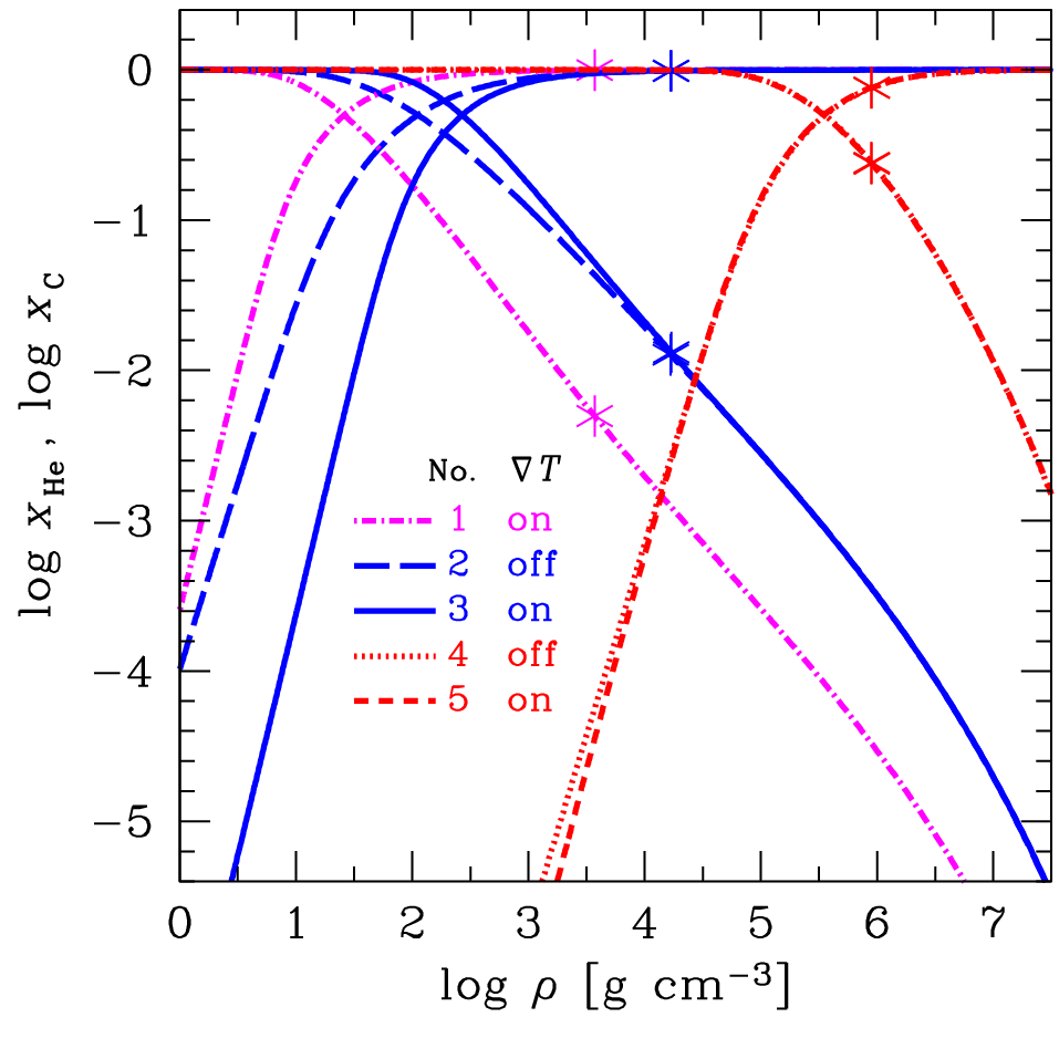
Fig. 16 demonstrates the effect of the terms containing in Eqs. (6.1) or (7.2) on the properties of He – C envelopes. The figure shows the fractions of helium, , and carbon, , calculated in five cases (curves 1 – 5) for one and the same surface temperature MK. The left part of this figure (at ) should be taken with caution, because the matter at these densities is non-degenerate (according to Eq. (4.13), g cm-3), so that the involved assumptions (such as the linear mixing rule), which are applicable for strongly degenerate plasmas, are no longer valid there. Curves 1, 3 and 5 are computed including the contribution of terms, whereas curves 2 and 4 neglect this contribution (which is equivalent to the approximation made in Section 6 and in the paper by Chang et al. 2010). Curves 2 and 3 are computed for one value of g cm-3, whereas curve 1 assumes the same fraction of carbon at the radiative surface (from which one integrates the equations), as curve 2, . This boundary condition leads to a different value of the accumulated mass of helium, and therefore to a different g cm-3. Nevertheless, the difference between curves 1, 2 and 3 has almost no effect on the relation. The values of for these relations differ by less than 1% because the corresponding values of lie out of the sensitivity strip. In contrast, curves 4 and 5 have g cm-3 inside the sensitivity strip. However, in this case the effects of are weak owing to stronger electron degeneracy (as already mentioned in Section 6.2, in the approximations of linear mixing, strongly non-ideal ion plasma, and strongly degenerate electrons, all the terms disappear). That is why curves 4 and 5 are close to each other and the terms, again, do not affect the relation.
As seen from curves 1, 2 and 3, the contribution of the term depends, among other things, on the statement of the problem. It is important which quantity is fixed as a boundary condition – the accumulated mass or the fraction of ions at the surface. According to calculations, the terms have the strongest effect on the ion fraction profiles if the transition region coincides with the region of moderate coupling of ions. This situation occurs at sufficiently high in the outer regions of the envelopes ( g cm-3) which consist of light elements (such as hydrogen, helium, carbon). However even in these cases the effect of on the relations, profiles of pressure, temperature and density is weak.
7.4 Envelopes out of diffusive equilibrium
In addition to diffusively equilibrated heat blanketing envelopes, Beznogov et al. 2016b considered the envelopes out of diffusive equilibrium. Since ion diffusion is relatively slow (see below), a non-equilibrium state can exist for a long time without violating a global hydrostatic equilibrium. By way of illustration, let us study a fixed ion distribution, , ignoring the equations of diffusive equilibrium. The structure of the envelope can be calculated by integrating Eqs. (7.3).
The results are presented in Fig. 17. The left panel shows three envelope models for H – He mixtures. The right panel presents three models for He – C mixtures. The figures demonstrate the helium number fraction as a function of mass density for the canonical neutron star model with surface temperature K. All three models for the H – He mixtures have the same amount of hydrogen (), while all three models for the He – C mixture have the same amount of helium (). The helium fraction increases with on the left panel, because helium is heavier than hydrogen, but it decreases on the right panel since helium is lighter than carbon. The solid lines refer to diffusion-equilibrated configurations, while the dashed lines refer to non-equilibrated configurations with wider (long dashes) and narrower (short dashes) transition regions, than in the equilibrated case.


All three models give nearly the same values of . For instance, for the He – C mixture, one gets the temperature K at g cm-3. For the H – He mixture at g cm-3 one has K for the equilibrium and “narrow” profiles and K for the “wide” profile. Therefore, the resulting relations are weakly sensitive to a heat blanket configuration. The main parameter which regulates the relation is the accumulated mass of light elements divided by (or, equivalently, or ). This is true at least as long as the ion distributions are not too wide, as seen for the H – He mixture, for which the “wide” profile gives a slightly different value of . On the other hand, strong deviations from an equilibrium configuration cannot exist for a long time (see below).
The insensitivity of the relations to the distribution of ion fractions is helpful for understanding the importance of thermal diffusion effects. Although thermal diffusion may change ion fractions, these changes will not affect the resulting relations. However, thermal diffusion can be important for the processes that are sensitive to the distribution of the ion fractions (e.g., diffusive nuclear burning). Beznogov et al. 2016b demonstrated this by making several estimates, assuming a constant thermal diffusion ratio in Eq. (6.12), which is the conservative upper limit obtained in calculations with the effective potential method. For the H – He mixture with , the thermal diffusion rate does not exceed 3% of the ordinary diffusion rate, and for the He – C mixture () it does not exceed 6%.
Using Eq. (6.20), one can calculate the diffusion velocity of ions for diffusively non-equilibrium configurations considered in Fig. 17. Then, introducing a typical width of the diffusively non-equilibrium layer and taking characteristic diffusive velocities , one can estimate typical diffusion-equilibration time for these configurations. For the H – He envelopes, the estimate gives about a few meters, the diffusive velocity cm s-1 and the diffusion-equilibration time of a few days or weeks. For the He – C envelopes, is also about a few meters but the diffusion velocity is much slower, cm s-1. Accordingly, yr. The equilibration in the He – C mixture lasts much longer as a result of the slow Coulomb separation of ions. Therefore, the diffusive equilibration takes from a few days to a century, depending on the chemical composition of heat blankets.
7.5 Diffusive and the onion-like heat blanketing envelopes
Let us compare the main properties of the diffusive (Section 7) and onion-like (PCY97, Section 5) blanketing envelopes. For illustration, we consider a canonical neutron star with the effective surface temperature MK. Then the redshifted surface temperature is MK. This choice corresponds to the magnetic hydrogen atmosphere plus power-law fits to the Vela pulsar spectrum from Chandra observations by Pavlov et al. 2001 and from observations by Manzali et al. 2007. Recently Ofengeim and Zyuzin 2018 obtained a similar value MK for Chandra observations. It is remarkable that the attempts to improve the estimate using wide ranges of and give almost the same in all these ranges (e.g., Ofengeim and Zyuzin 2018). Using a relation, one can determine the non-redshifted temperature at the envelope bottom and the redshifted internal temperature of isothermal stellar interiors . In reality, the Vela pulsar possesses the surface magnetic field G. Therefore, the distribution over its surface is non-uniform (see Section 8.3.4), which was ignored in the above-mentioned spectral models.

Fig. 18 shows the dependence of the internal stellar temperature on the accumulated mass of lighter elements in the blanketing envelope for different envelope models. The short-dashed curve corresponds to the envelope composed of He – C mixture with g cm-3. It demonstrates the dependence of on the total mass of helium, . The long-dashed line shows the same but for C – Fe envelopes, with being the total mass of carbon. The dash-dot line refers to H – He envelopes, being the total mas of hydrogen; in this case g cm-3, , because hydrogen cannot survive at higher densities (cf. Section 3.3.2). The solid line is calculated for the PCY97 model with g cm-3, and is the total mass of H and He.
This figure is analogous to Fig. 15 in Section 7.3. It also shows the “anomalous” behavior for the H – He mixture. For other envelope models, the thermal conductivity and internal temperature increase with the growth of at a fixed surface temperature (see Section 7.3 for details). According to Fig. 18, if the chemical composition of the envelope is unknown, theoretical uncertainties of due to unknown are really large and hamper an accurate determination of . The largest variation by a factor of is achieved for the PCY97 model. This has been anticipated, because the PCY97 model assumes the presence of larger spectrum of chemical elements. For binary mixtures, especially, for the H – He and He – C envelopes, the variations of are smaller. This is also natural, because the difference of charge numbers of ions in the binary mixtures is smaller, hence variations of heat conduction are weaker.
Since different curves in Fig. 18 are plotted for of different nature, a plain comparison of the curves may be misleading. However, in some cases such a comparison is possible. For instance, the PCY97 and He–C curves at correspond to the blankets which are mostly composed of He; these curves are in very good agreement with each other. Equally, the PCY and C–Fe curves at low correspond to the blankets almost fully composed of Fe; they are also in good agreement.
Fig. 19 shows thermal states of the same star as in Fig.18 but at different (when the star is warmer or colder) for different models of the heat blanketing envelopes. The thermal states are characterized by the dependences of on which, in their essence, are analogous to the dependences of on (Fig. 14). The vertical dotted line marks K (as in Fig. 18). The curves can be viewed as “evolutionary tracks” of the star. The left panel is devoted to He–Fe and He–C envelopes; the thick curves refer to one-component envelopes (the thick dashed curve is for pure Fe, the solid curve for pure C, and the dot-dashed curve for pure He). Thin curves of different styles correspond to binary mixtures with different masses of lighter ions (, , , and ). The lowest value of corresponds to a thin surface layer of a lighter element, while the highest value to a thin layer of a heavier element at the bottom of the heat blanket. The relations vary in response to the variations of the envelope’s composition.


The right panel of Fig. 19 demonstrates the same as the left panel but for the PCY97 model. As before, the thick dashed line corresponds to the envelope of pure iron. The thick solid line (denoted as “Acc”) is for the envelope with the maximum amount of H+He. Thin dashed lines of different styles refer to different masses of H+He. As expected, this model gives the widest variations of , which is clear from comparison of the right and left panels of Fig. 19. Notice that difference in the values of for a partially accreted and non-accreted envelopes is smaller in warmer stars and larger in colder stars, which is explained by the shift of the sensitivity strip to lower densities as the star cools down.
The most important result is that the relations for the diffusive envelopes are nearly independent of the structure of the transition layer (on its width, distributions of ion fractions, presence or absence of diffusive equilibrium). These relations depend only of (or ). In particular, these results confirm the validity of the PCY97 models (Section 5), where the envelopes were approximated by the sequence of shells of ions of one species (that is of H, He, C or Fe), with sharp boundaries between the shells (the “onion-like” structure).
To summarize our comparison of the diffusive models of heat blankets with the PCY97 models we would like to stress the following:
- 1.
Binary-mixture diffusive and PCY97 models are based on almost the same microphysics. They are not diverse but complementary.
- 2.
One can use the PCY97 model if the composition of a given blanketing envelope is formed via the quasi-stationary evolution of accreted hydrogen-helium matter (with the layers of H, He, C, and Fe from top to bottom). At the heat blanket will be fully accreted (H, He, C). The position of the upper boundary of the Fe layer can be shifted upwards by decreasing . While using the PCY97 fits presented in Section 5.5, one should bear in mind that the positions of the interfaces between different elements are fixed. If these positions are different, a heat blanket model should be recalculated.
- 3.
PCY97 stated that replacing hydrogen with helium and carbon with iron would have almost no effect on relations. Here we have paid more attention to the effect of such replacement and confirmed that the effect is small, compared with a replacement of light ions (H or He) by heavier ones (C or Fe).
Nuclear reactions in the blanketing envelope can noticeably change and the relation in the course of a neutron star evolution. All the calculations in this section have neglected the possibility of convection in the envelope. As discussed in Section 5.3 (see Fig. 2), the convection can occur in some parts of the envelopes, but it has almost no effect on the relations.
The calculated relations for diffusively equilibrated envelopes have been approximated by analytic expressions (Appendix B), which are convenient for simulating thermal evolution of neutron stars and related phenomena.
The presented models of heat blankets are greatly simplified; real envelopes may contain ions of many species. For example, Fantina et al. 2020 studied the cooling and the equilibrium composition of the outer layers of a non-accreting neutron star down to crystallization and showed that the sharp changes in composition obtained in the one-component plasma approximation are smoothed out when a full nuclear distribution is allowed. In the liquid part of the envelope, however, stratification of ions will prevent the appearance of regions containing many ion species at once. Realistic envelopes have most probably shell structures with one type of ions in each shell and narrow diffusive transition layers of binary mixtures between the shells. For calculating relations, it would be sufficient to neglect diffusive broadening of the shell boundaries. However, the “onion-like” approximation could be insufficient for tracing the evolution of nuclear composition within the blanketing envelopes, for example, with allowance for the diffusive nuclear burning (Chang and Bildsten 2003; Chang and Bildsten 2004; Chang et al. 2010; Wijngaarden et al. 2019).
8 Magnetic blanketing envelopes
8.1 Statement of the problem
8.1.1 Microphysics of matter in magnetic envelopes
Microphysical properties of the matter in magnetic heat-blanketing envelopes have been described in many publications (see, e.g., Yakovlev and Kaminker 1994; Potekhin and Chabrier 2013; Potekhin et al. 2015b, and references therein). In this section we briefly outline some important results.
Magnetic fields in the heat blankets affect the properties of electrons and ions. As a rule, the effects on the properties of electrons are most pronounced. These effects can be roughly separated in two types. First, there are classical effects associated with electron rotation about -lines. Secondly, there are quantum-mechanical effects produced by quantization of electron motion across and resulted in the appearance of the electron Landau (or Rabi-Landau88 8 The magnetic quantization was first studied by Rabi 1928.) energy levels. The quantum effects are usually pronounced at much higher magnetic fields than the classical ones. The classical effects change mainly the electron transport properties but leave the thermodynamic properties (e.g., the electron pressure) unchanged. The quantum effects can modify the transport and thermodynamic properties. The effects of both types can be different in non-degenerate and degenerate electron plasmas.
Classical effects
The most important classical effect is that electron conduction becomes anisotropic. The effect occurs at any electron degeneracy and is controlled by the electron magnetization parameter
| (8.1) |
where is the effective electron thermal-conduction relaxation time, is the characteristic gyrofrequency of rotation of a conduction electron about the magnetic field lines, is the electron cyclotron frequency, and is the characteristic Lorentz factor of the conduction electrons. In the degenerate matter, , with being determined by Eq. (3.13). In this case, where G.
The electron heat conduction in a magnetic field is determined by the three thermal conductivity coefficients, specifically, by the thermal conductivities and along and across , and by the Hall thermal conductivity which describes the heat flux component perpendicular to and to the temperature gradient . If the quantum effects are small, the conductivity appears to be almost independent of . In the regime of weak electron magnetization (, many collisions during one gyro-rotation) the electron conduction is only slightly anisotropic, with and . In the opposite case of strongly magnetized electrons (, many rotations between successive collisions), and , so that thermal conduction across -lines becomes greatly suppressed. Therefore, the magnetic field can significantly affect the electron heat transport at .
Quantum effects
In non-degenerate layers of neutron-star envelopes, the electrons are usually non-relativistic; electron thermal conduction is relatively unimportant because radiative thermal conduction is sufficiently high (resembling the non-magnetic case; e.g., Section 4). The magnetic field is called strongly quantizing for the electrons, if it forces the majority of the electrons to occupy the ground Landau level. In a non-degenerate matter, this occurs at , where
| (8.2) |
However, in the non-degenerate case the electron pressure still remains unaffected by , being equal to , although some other thermodynamic functions are affected (for instance, the electron heat capacity is reduced by a factor of 3). As for the radiative thermal conductivity, it becomes anisotropic. It is described by the two radiative thermal conductivity coefficients, along and across , which are enhanced, as compared to the non-magnetic case, proportionally to .
In the deeper layers of the heat blanket the electrons become strongly degenerate (and possibly relativistic); the anisotropy of electron thermal conduction is most important. It operates in the classical and quantum regimes. In the quantum regime, the magnetic field modifies also the electron gas thermodynamics, particularly, .
The quantum effects of magnetic field are different in the two domains of and (for details see, e.g., Haensel et al. 2007, Chapter 4). The first is the domain of strongly quantizing magnetic field, which forces almost all the electrons to occupy the ground Landau level. It occurs at relatively low and low , where
| (8.3) |
In this case all thermodynamic and kinetic properties of the electron plasma can be strongly affected by the magnetic field. The second is the domain of weakly quantizing field, where and . In this domain the electrons can populate many Landau levels but the thermal energy is smaller than the distance between neighboring Landau levels. Then the presence of the Landau levels can still affect thermodynamic and kinetic properties of the electron plasma. The bulk properties like the electron pressure, internal energy, or chemical potential are affected only slightly. If very high accuracy is not required, they can be replaced by corresponding non-magnetic quantities. However, those quantities that are determined by the electrons with energies near the Fermi energy (for instance, electron specific heat or transport coefficients) can be affected much stronger. Such quantities oscillate with increasing density due to population of new Landau levels by strongly degenerate electrons.
At the quantizing magnetic field strongly reduces the degeneracy temperature,
| (8.4) |
where is given by Eq. (3.14), and is the Fermi momentum of degenerate electrons in the strongly quantizing limit in units of .
In summary, the strongest effects of a magnetic field on the microphysics of plasma in heat blanketing envelopes are expected at sufficiently low densities and temperatures, and . For instance, at G, one has K and g cm-3. If is more or less the same within the envelope and we increase or beyond or , the magnetic effects will weaken. In a weakly quantizing field, the quantum effects make the thermodynamic functions to oscillate around their classical values with changing or (Potekhin and Chabrier 2013, see).
8.1.2 Magnetic heat blankets for 1D and 2D thermal evolution codes
High magnetic fields make thermal conduction in the outer layers of neutron stars strongly anisotropic. This affects thermal flows near the stellar surface and the surface map of the effective temperature . In addition, the magnetic forces and quantum effects of the -field on the pressure can change the hydrostatic structure of neutron star layers. The problem of neutron star thermal evolution ceases to be one-dimensional (1D) and becomes more complicated (2D or even 3D).
It seems reasonably to assume that the blanketing envelope remains thin and can be artificially divided into small domains in such a way that is nearly constant in each domain (varying parametrically from one domain to another). Let us assume further that typical length-scales of these domains along the surface are much larger than the heat blanket width. Then one can approximate any domain by a piece of plane-parallel layer (like in Section 3.2), solve the corresponding heat transport problem and find a local relation. Here, and are, respectively, the local surface and internal temperatures for a given domain. Generally, both temperatures depend on the magnetic field in the given domain.
The solution of the above problem for all domains can be used as a boundary condition to model (Section 3) the thermal and magnetic evolution in neutron star interiors ().
Naturally, the magnetic field penetrates into the entire star or into its essential part, the crust and the core. Then the magnetic effects, particularly, anisotropic heat conduction, have to be included into the equations which describe the thermal and magnetic evolution of the interiors. In this connection, one can employ the two heat-blanket descriptions which are good either for 2(3)D or for 1D thermal evolution codes.
Heat blankets for 2D or 3D codes
These 1D heat-blanket models based on the heat transport solutions for separate domains can serve as boundary conditions at appropriate internal domains in 2D or 3D codes to follow the thermal evolution of magnetic neutron stars.
Heat blankets for 1D codes
The 1D heat-blanket models provide natural boundary conditions for the 1D evolutionary codes. Their use can be based on the assumption that neutron star interiors are isothermal; see Eq. (2.16) and the discussion in Section 3.2. The isothermality can be provided by high conductivity of the stellar interior, if the thermal evolution time-scale is sufficiently long. The weaker assumption that depends only on , but not on the angles in the spherical coordinate system, is also sufficient. This weaker assumption can be fulfilled, if the heat conduction at is isotropic and the thermal relaxation time of the non-isothermal zone is small compared to the thermal evolution time-scale. There may be several causes for this isotropy: the decrease of the Hall parameter with increasing density, a small-scale (compared to ) configuration of the magnetic field, or predominant conduction by neutrons if reaches the neutron-drip density (as in Potekhin et al. 2003).
Then is the same in all the domains of the envelope at a given moment of time. Therefore, one can integrate over all the domains and obtain the total photon surface thermal luminosity as a function of . The relation, derived in this way, plays the same role as the relation for non-magnetic stars. In this case, it is convenient to define the mean effective surface temperature by
| (8.5) |
and use the relation to study the thermal evolution of the star with a 1D computer code. The heat blanket remains essentially 2D, but the anisotropic temperature distribution in the heat blanket is totally included in the appropriate relation, making the internal thermal evolution problem one-dimensional.
Now the surface distribution of the effective temperature can be noticeably non-uniform and the observable radiation flux can depend on observation direction. However, we will see (Section 8.3.6) that the effect is almost smoothed out due to light bending in General Relativity, at least for a dipole surface magnetic field and isotropic local surface emission model. A distant observer will detect nearly the same bolometric thermal flux observing the star at any angle.
1D versus multi-D
Since 2D or 3D codes are more complicated, they are used less often. A review of such computations is given by Pons and Viganò 2019. For example, a 2D code has been realized by Aguilera et al. 2008 and elaborated by Viganò et al. 2013.
1D codes are simpler; they have been employed in the majority of studies of cooling magnetized neutron stars. Their validity is restricted by the requirement that is independent of angles at , as discussed above. This requirement does not necessarily imply that the effects of magnetic field in the interiors are washed out (for instance, the heat transport is isotropic or the generation of Joule heat due to the electric current dissipation is spherically symmetric). The isothermality can be provided by the high thermal conductivity even for anisotropic heat transport, sources, or sinks. Then the main places of anisotropic temperature distribution are the heat insulating envelopes. In these envelopes, the magnetic effects can be especially strong and the heat conduction is not too fast to smear out the anisotropy.
It would be difficult to formulate strict conditions for the validity of 1D codes. These conditions depend on specific problem, particularly, on magnetic field strength and geometry. We expect that 1D codes are especially accurate if the magnetic field in the neutron star crust is G.
In what follows we mainly discuss the heat blankets for 1D codes.
Constructing magnetic heat blankets
At the first step one needs to solve a heat blanket problem in a small local part of the insulating envelope. If we assume a locally constant within this part, we will have no magnetic force there and the hydrostatic equilibrium will be described by our familiar Eq. (3.2), although the pressure can depend on due to the quantum effects outlined in Section 8.1.1.
As we discussed above, the heat transport in the magnetic heat blanket is generally described by the three thermal conductivity coefficients: , , and . Nevertheless, one can show that, in our approximation of a local thin plane-parallel blanket with a locally fixed , Eq. (3.4) remains valid, if means the effective radial thermal conductivity, given by
| (8.6) |
where is the angle between and the normal to the surface. Therefore, the problem for a local domain reduces to solving the same two equations (3.2) and (3.4), which have been used for non-magnetic heat blankets, but with more complicated physics involved.
The magnetic field affects the thermal structure of the blanketing envelope in several ways (Section 8.1.1). First, it makes the thermal conductivity anisotropic. Here, the effects are twofold.
(i) Classical effects of electron rotation about field lines can strongly reduce but they do not affect . They are especially important near the magnetic equator [, in Eq. (8.6)]. Such equatorial regions become poor heat conductors, which lowers the local effective temperature for a given .
(ii) Quantization of electron motion into Landau levels can strongly modify both and . If the heat is mostly transported by degenerate electrons and the magnetic field is strongly quantizing, then the quantum effects enhance . These effects are most pronounced near the magnetic poles, where and . Then the quantum effects increase the local for a given .
In the domains of strongly quantizing magnetic field, the classical and quantum effects on thermal conduction act in opposite directions. They are mainly important in different parts of the neutron star surface. In addition, one needs much stronger -fields to make the quantum effects pronounced. Note that the quantum effects modify also the plasma pressure, and hence the profiles.
The approximations of the model
Evidently, the formulated heat blanket model is not perfect. First of all, the approximation of locally constant (force-free) magnetic fields can be too crude. Indeed, the field in the outer neutron star layer is likely to be nearly force-free, but even relatively small corrections may produce magnetic forces which could affect the structure of the outer layers.
Second, the formulated model deals actually with radial heat fluxes. Within the same model, there are also tangential fluxes. Such fluxes may be insignificant at one domain of the surface, but combining the domains we will obtain heat fluxes circulating under the surface. They can be locally constant along their circulation lines. However, globally, tangential heat circulations may redistribute some amount of heat from one domain of the heat blanket to others and affect thus . For example, in the dipole field model, the heat is transported along the field lines from hotter polar regions to cooler equatorial domains, so that the equator temperature becomes higher than predicted by the plane-parallel approximation. This becomes important in superstrong magnetic fields G (e.g., Potekhin et al. 2015b). However, this can hardly affect the observed luminosity, because, in strong magnetic fields, the equatorial region is cold and gives negligible contribution to the total flux anyway. One can also anticipate that the temperature gradients along the surface may render some parts of the envelope baroclinically unstable, although a strong magnetic field may partly stabilize it.
Such effects have been almost not considered in the literature and will be ignored below. They could be good subjects for future projects.
8.2 Analytic model
The main effects of strong magnetic fields on the heat blankets can be understood using a simplified fully analytic model, analogous to that considered in Section 4 for the non-magnetic case. For a strongly quantizing magnetic field, such a model was constructed by Ventura and Potekhin 2001; it is outlined below. Many results are useful for understanding the main features of the heat blankets for 2D codes. More elaborated numerical models are discussed in Section 8.3, mostly for the heat blankets designed for 1D codes.
8.2.1 Equation of state
As in the non-magnetic case, we consider the envelope composed of a fully ionized electron-ion plasma. The equation of state of such a plasma has been discussed in Potekhin and Chabrier 2013.99 9 See footnote 2 on page 2. Under typical conditions in the heat blanketing envelopes, the Landau quantization of ion motion can be neglected, whereas the electrons can be quantized.
First consider the case of low temperatures, where the electrons are degenerate. As mentioned in Section 8.1.1, in the regime of weak quantization, the electron pressure oscillates around its non-magnetic values with increasing density. Replacing the accurate EoS by its non-magnetic counterpart will not noticeably affect the structure of the envelope.
In the strongly quantizing limit ( and ) the pressure of degenerate electrons becomes much lower than at . As a result, the electrons remain non-degenerate along the radiation-dominated part of the envelope. Since the pressure of the non-degenerate gas is independent of the magnetic field, we can use the classical non-degenerate EoS in this part of the envelope.
8.2.2 Radiative opacities
The radiative thermal conductivity in a magnetized plasma was described, e.g., by Potekhin and Chabrier 2018. The radiative conductivity becomes anisotropic (Section 8.1.1), but the difference between its longitudinal () and transverse () components is not too large, so that we can neglect the difference for a qualitative analysis. If the radiative opacities are mediated by free-free transitions, then in a strongly quantizing magnetic field they tend to
| (8.7) |
where is given by Eq. (4.3), is given by Eq. (8.4), and is expressed in g cm-3. This estimate may be used if only and . We will use it in Section 8.2.4. According to Eqs. (3.11) and (8.7), the strong magnetic fields, , push the radiative surface to higher densities, .
| 1 | 2 | 3 | 4 | 5 | 6 | |
|---|---|---|---|---|---|---|
| 0.0949 | 0.1619 | 0.2587 | 0.3418 | 0.4760 | 0.2533 | |
| 0.0610 | 0.1400 | 0.1941 | 0.0415 | 0.3115 | 0.1547 | |
| 0.090 | 0.0993 | 0.0533 | 2.15 | 0.2377 | 0.231 |
Another approximation, which takes both free-free transitions and Thomson scattering into account, has been developed by Potekhin and Yakovlev 2001 following numerical calculations of Silant’ev and Yakovlev 1980. At fixed and , it reads
| (8.8) |
where
Here, mass density is measured in g cm-3, and are the Rosseland opacities in a strongly quantizing magnetic field for propagation of photons along and across , respectively, which are related by Eq. (3.8) to and in Eq. (8.6); is the Thomson scattering opacity at (determined by the Thomson scattering cross section ), , where eV is the Rydberg energy; is the free-free opacity at . The fit parameters , and given in Table 1 ensure an average fit error of 5.5% with the maximum error of 11% to the numerical results of Silant’ev and Yakovlev 1980. The factor , which effectively eliminates the radiative transport at large densities, has been introduced by Potekhin et al. 2003; it mimics the suppression of radiative transport at photon frequencies below the electron plasma frequency.
The scattering opacities are modified by the electron degeneracy at high and by the Compton effect at K. An accurate analytic description of both these effects is given by Poutanen 2017. The free-free opacities are suppressed by electron degeneracy. In the absence of the Landau quantization, the free-free opacities at arbitrary degeneracy have been fitted by Schatz et al. 1999, based on numerical calculations of Itoh et al. 1991. The fit of Schatz et al. 1999 is inapplicable in the case of quantizing magnetic fields. On the other hand, the fit (8.8) is only applicable for non-degenerate non-relativistic plasmas. A smooth interpolation between the different regimes has been suggested by Potekhin and Chabrier 2018.
Caution is necessary however while using these fit expressions. A strong magnetic field shifts the ionization equilibrium toward a lower ionization degree by increasing the electron binding energies. Therefore, even if the plasma is fully ionized at some and in the absence of the magnetic field, it can be only partially ionized at the same and for high . This increases the contribution of bound-bound and bound-free transitions and can increase the radiative opacity well above the values given by Eq. (8.7) (Potekhin et al. 2015a, see).
8.2.3 Electron thermal conductivities

Unified expressions for the electron thermal conductivities in a fully ionized degenerate plasma with arbitrary magnetic field are discussed, e.g., in Potekhin et al. 2015b. As we already mentioned in Section 8.1.1, these conductivities undergo quantum oscillations at . At G, the electron transport across the field is typically suppressed by orders of magnitude. This allows one to neglect , which is a good approximation everywhere except in the domains where . In this approximation, Eq. (8.6) reduces to
| (8.9) |
This formula holds not only in the degenerate but also in the non-degenerate electron gas. In the simplest approximation, in which the effective electron relaxation time is calculated for fully degenerate matter, the conductivity decreases and increases towards lower densities at , as is shown in Fig. 20. However, averaging over the finite thermal width of the Fermi level terminates the growth of and moderates the decrease of , before they become comparable.
In order to construct a temperature profile, we can calculate in the classical (non-magnetic) approximation (4.16) at high densities, where the magnetic field is weakly quantizing. At lower densities, the quantizing nature of the field must be taken into account. At , as long as the electrons are strongly degenerate and the ions form a strongly coupled Coulomb liquid, one obtains the order-of-magnitude estimate (Ventura and Potekhin 2001, see)
| (8.10) |
where is magnetic field strength in relativistic units, is the non-magnetic conductivity given by Eq. (4.16), and is the non-magnetic Coulomb logarithm. This estimate gives the values of not much different from numerical results, provided that and .
As noted above, very strong fields push the onset of electron degeneracy to higher . Therefore, the turnover from radiative to electron thermal conductivity may occur in the non-degenerate regime. In that case, can be evaluated from Eq. (4.15).
8.2.4 Temperature profile
In Section 8.1.1, we have defined several regimes regulating the EoS and opacities in strong magnetic fields. To construct an approximate analytic temperature profile, it is sufficient to use the non-magnetic radiative and longitudinal electron thermal conductivity unless the field is strongly quantizing. Magnetic oscillations around the classical thermal conductivities will be smoothed out by integration while obtaining the temperature profile from Eq. (3.4).
In the domain of strongly quantizing magnetic field, the opacities are appreciably modified. However, in the liquid degenerate part of the heat blanket, which is of our primary interest here, the analytic expressions for can be again approximated by a power law, Eqs. (8.10) and (4.15). As follows from Eq. (8.7), the same is true for the radiative opacity in the extreme quantizing limit (provided that the free-free opacity dominates). In the non-degenerate regime, the magnetic field does not affect the EoS. In this case, we recover the solution given by Eq. (4.6) with the new values of and ,
| (8.11) |
where is given by Eq. (4.11). Thus the temperature is reduced (its profile becomes less steep) with increasing as long as the field is strongly quantizing ( and ).
Interestingly, the value of the constant conductivity along the thermal track, Eq. (4.7), is independent of the magnetic field, while its numerical value is only slightly lowered as a result of changing the parameter .
8.2.5 Sensitivity strip
As in the non-magnetic case, the sensitivity strip is placed near the point, where , and the radiative conduction is overpowered by the electron one. In a strongly quantizing field, using Eqs. (8.7) and (8.10), we have
| (8.12) |
instead of Eq. (4.17). With the temperature profile (8.11), we now obtain
| (8.13) |
If, however, the electrons are non-degenerate along the turning line, then is given by Eq. (4.15) instead of Eq. (8.10), and we obtain the turning point at
| (8.14) |
Combining with Eq. (8.11), we get
| (8.15) |
Thus, in the cases of degenerate and non-degenerate electrons we obtain quite similar expressions for and . Comparing them with Eq. (4.18) we see that in the non-magnetic case has the same order of magnitude as in the magnetic field at . However increases with increasing in the magnetized envelope. Notice that in a strongly quantized magnetic field is independent of the field strength, while grows linearly with . One can see that lies in the region of strong magnetic quantization. Assuming that is not close to and neglecting the factors about unity, we see that for , which corresponds to the high-field pulsars and magnetars (Section 10.2).
Let us also estimate the point at which the electrons become degenerate. For simplicity, we assume that the electrons are non-relativistic. Note that the condition in the strongly quantizing magnetic field is equivalent to g cm-3. Then from Eq. (8.11) we obtain
| (8.16) |
Thus, in analogy to the non-magnetic case, turning from radiative to electron thermal conduction occurs not far from the degeneracy onset, . Depending on , it occurs either in the non-degenerate (at ) or in the degenerate (at ) electron gas.
The integration of the temperature profile beyond the turning point (for obtaining ) can be done in the same way as in the non-magnetic case. However, the integration path should be divided in two parts: (i) , where Eq. (8.10) for the thermal conductivity can be used, and (ii) , where Eq. (4.19) can be used with the right-hand side divided by . The result is similar to Eq. (4.20), but contains a profound dependence on the inclination angle: the thermal gradient grows rapidly as approaches .
8.3 Numerical results
We will mainly outline the models for heat blankets made of iron (Potekhin and Yakovlev 2001) and of partly accreted (PCY97-like) matter (Potekhin et al. 2003). Since the isothermality in high- fields may be reached at larger , the bottom density in these models is shifted to g cm-3. The analytic fits for magnetic models are constructed in such a way to reproduce the fits derived (Section 5.5) for at g cm-3. The models are designed for 1D codes. The results for G are illustrative (may be improved with 2D or 3D codes, as discussed above; it was demonstrated, for instance, by Potekhin et al. 2015b).
8.3.1 Equation of state and opacities
In the deep layers of the blanketing envelope, where the plasma is fully ionized, the pressure is mostly determined by free electrons with small corrections due to ions (Chapter 4 of Haensel et al. 2007). The transport properties of such a plasma have been reviewed by Potekhin et al. 2015b.
A considerable complication at lower densities is introduced by bound species. As discussed in Chapter 4 by Haensel et al. 2007, different approaches to the EoS yield appreciably different models of atmospheric layers. We will mainly use the models of iron (non-accreted) blanketing envelopes based on the Thomas-Fermi EoS derived by Thorolfsson et al. 1998.

8.3.2 Temperature profiles
Fig. 21 shows the calculated temperature profiles in the envelopes of neutron stars at three surface magnetic fields, G, G, and G, two effective surface temperatures, MK and 2 MK, and five angles between the field and the normal to the surface, from 0 to 90∘. The curves start at the radiative surface, where . These results confirm the qualitative conclusions of Section 8.2. Strong dependence on the magnetic field inclination, , starts to be pronounced near turning points. In accordance with our estimates (Section 8.2), they are shifted to higher densities with increasing . The linear dependence of the radiative-surface density, , obtained analytically, is seen to be realized for G.
The higher the temperature, the wider is the density region, where and do not differ strongly from the scalar thermal conductivity at . Therefore the dependence of the profiles on the magnetic field is less pronounced at higher showing convergence to the case.
The temperature profiles, which are calculated with allowance for neutrino emission (solid and dashed lines), are compared with the results of calculations assuming (dotted lines). In the domains where the difference between these results is noticeable, the thermal flux is not constant through the envelope, so that Eq. (3.6) is not applicable.
It should be noted that the profiles in Fig. 21 have been calculated assuming a neutron-star photosphere without phase transitions. However, some theoretical results hint that the strong magnetic field may cause the so-called magnetic condensation, which implies formation of a physical solid or liquid surface instead of imaginary radiative surface inside an extended atmosphere (see Medin and Lai 2007 and references therein). Potekhin et al. 2007 compared thermal profiles with and without the magnetic condensation and demonstrated that the effect of the condensation on the relation is small (see their Fig. 7). Nevertheless, this effect can be visible on the neutron star cooling curves (Potekhin and Chabrier 2018).
8.3.3 Surface temperature at the magnetic pole and equator
The relation between the internal and surface temperatures, considered for non-magnetic envelopes in Section 5.5, is strongly affected by the magnetic fields (Fig. 21). To study these effects we introduce the ratios of the surface temperature at a given field to the value at for the same .
| Iron envelope | Accreted envelope | |||
|---|---|---|---|---|
| 1 | 159 | 172 | ||
| 2 | 0.038 | 270 | 0.055 | 155 |
| 3 | 1.5 | 172 | 2.0 | 383 |
| 4 | 0.0132 | 110 | 0.0595 | 94 |
| 5 | 0.620 | 0.363 | 0.328 | 0.383 |
| 6 | 0.318 | 0.181 | 0.237 | 0.367 |
| 7 | 0.50 | 2.28 | ||
| 8 | 3 | 0.619 | 2 | 1.690 |
| 9 | 0.160 | 0.113 | ||
| 10 | 21 | 163 | ||
| 11 | ||||
Let us start with the two most important cases of the magnetic field which is either normal or tangential to the surface (i.e., at the magnetic pole or equator, respectively). In the first case the heat is transported through the heat-blanketing surface by the longitudinal thermal conductivity along the magnetic field lines, ; we will call this case the parallel conduction case. In the second case the heat is transported by the transverse thermal conductivity across the field lines, , which will be referred to as the transverse conduction case. Extensive calculations of the temperature profiles for both cases have been performed by Potekhin and Yakovlev 2001 in the case of iron envelope and by Potekhin et al. 2003 for partially and fully accreted envelopes. These authors produced the following analytic fits:
| (8.17) | |||||
| (8.18) |
with the parameters and given in Table 2. Here, as before, . These fits were checked against calculations for input parameters restricted by the conditions , , and , where and are expressed in K and is G. The numerical values of are reproduced with residuals up to 5–10%. The authors emphasized that these results are uncertain at superstrong fields ( G).

The effect of the magnetic field on the local effective temperature is illustrated in Fig. 22. The figure shows the distribution of the redshifted temperature over the surface of the canonical neutron star with the dipole magnetic field versus the magnetic field strength at the pole. The upper and lower curves of the same style present at the magnetic pole and equator, respectively. The electron-quantization effects amplify the longitudinal thermal conductivity, which is fully responsible for the heat transport near the pole. These effects make the polar regions of the heat-blanketing envelope more heat-transparent, increasing for a given . On the contrary, the classical Larmor-rotation effects strongly reduce the transverse conductivity which is most important near the equator. The equatorial regions become less heat transparent, which lowers the local effective temperature. These results are in qualitative agreement with the earlier results of Van Riper 1988, Schaaf 1990, and Heyl and Hernquist 2001, although there are quantitative differences discussed by Potekhin and Yakovlev 2001.
8.3.4 Variation of temperature over the stellar surface
The dependence of on the angle is most easily described by the model of Greenstein and Hartke 1983 which implies a superposition of “longitudinal” and “transverse” heat fluxes:
| (8.19) |
This approximation has been used, e.g., by Page 1995, Shibanov and Yakovlev 1996, and Heyl and Hernquist 1998. Numerical calculations of Potekhin and Yakovlev 2001 confirmed that it accurately (within %) reproduces the dependence of on . However, a replacement of the power-law index 4 with according to
| (8.20) |
yields better accuracy (see Potekhin et al. 2003).
According to Eq. (8.20), the flux density for any angle is expressed through the solutions for the cases of parallel and transverse conduction. Using Eqs. (8.17) and (8.18), one can thus find the flux densities at arbitrary and for the iron () and fully accreted envelope (). For a partially accreted envelope, one can use the interpolation (5.10), which remains reasonably accurate for strong magnetic fields. With this solution, one can easily calculate the distribution of the flux density and the effective temperature [Eq. (5.12)] over the neutron star surface for any strength and geometry of the surface magnetic field.
Consider, for instance, a dipole surface magnetic field (Ginzburg and Ozernoy 1964),
| (8.21) |
where is the polar angle of a local element on the surface measured from the magnetic axis, is the field strength at the pole, and is a factor due to General Relativity,
| (8.22) |
where
| (8.23) |
One has in the flat-space geometry ().
The distribution of over the surface of the star with a dipole magnetic field can be deduced from Fig. 22 (for K). This distribution drastically depends on the magnetic field strength. The fields G weakly affect the thermal conductivity and, hence, the surface temperature distribution. The fields G influence the transverse thermal conductivity much stronger than the longitudinal one due to the classical effects of electron Larmor rotation (Section 8.1.1). A wide equatorial region of the star becomes much colder than at while a smaller polar region becomes slightly warmer. For the higher fields, G, the situation is inverted: the increase of the longitudinal thermal conductivity by the quantizing magnetic field becomes more important. A large region of the surface with the center at the magnetic pole becomes hotter than at , but a narrow strip near the equator stays much colder than at . In this strip, the approximation of plane-parallel layer used for calculating the temperature profiles may become inaccurate. Large tangential heat flows may smear the temperature gradients in this equatorial “valley of the cold” which hopefully does not affect an overall surface temperature distribution.
Note that the anisotropy of the temperature distribution depends on the internal temperature . With increasing the anisotropy becomes smaller, as a result of the convergence to the case (Section 8.3.2).
8.3.5 Total photon luminosity
A relation is basic and extremely useful for non-magnetic neutron stars; is a reliable observable, and the relation allows one to infer . In a magnetic star, varies over the surface and is not a robust observable any more. Instead, it is more instructive to use the total surface luminosity of the star, , which seems to be really robust (see Section 8.3.6 below). The mean surface temperature can be conveniently defined by Eq. (8.5). In this way the relation in non-magnetic stars is replaced by the (or, equivalently, ) relation for magnetic stars.
The total photon luminosity is obtained by integrating the local radiated flux, , over the entire stellar surface. Potekhin and Yakovlev 2001 numerically calculated for iron blanketing envelopes with the dipole magnetic field and isotropic surface emission model and fitted the result as
| (8.24) |
where
and relates to the magnetic pole. The maximum fit error is 6.1% (i.e., 1.5% for the mean effective temperature ). Note that the fit expressions used by the authors for calculating were less accurate by themselves. This lowered the real accuracy of the presented fits. Nevertheless this accuracy seems sufficient for cooling simulations.

Fig. 23 displays the photon luminosity versus for two values of and four values of , mass of accreted matter in the blanketing envelope. The magnetic field affects the photon luminosity at G. In the range of G, the equatorial decrease of the heat transport dominates, and the luminosity is lower than at . For G, the polar increase of the heat transport becomes more important, and the magnetic field enhances the photon luminosity.
The joint effect of the accreted envelope and the magnetic field is demonstrated by the dot-dashed, dotted, and dashed lines. As in the non-magnetic case, the accreted material makes the envelope more heat-transparent, increasing the luminosity at given . Therefore, at – G, the magnetic field and the accreted envelope affect the thermal insulation in the opposite directions. At higher , both effects increase the luminosity. However, as evident from Fig. 23, the dependence of this increase on and is complicated. In particular, at G, the effect of the accreted envelope is weaker than in the non-magnetic case.
Note one important feature: the effect of the magnetic field on becomes weaker with growing . It is explained by the convergence to the solution discussed in Section 8.3.2. Accordingly, the luminosity of a hot neutron star cannot be strongly affected even by very high magnetic fields.
8.3.6 Gravitational lensing and observed flux
Since the temperature distribution over the surface of a magnetized neutron star is non-uniform, the flux of radiation detected from the star depends on observation direction. Calculating the flux, it is important to take into account gravitational bending of light rays propagating from the stellar surface to a distant observer. We will illustrate this effect of General Relativity for a spherically symmetric neutron star (with the Schwarzschild space-time geometry outside the star) using the results of Pechenick et al. 1983 and Zavlin et al. 1995b, and employing the heat-blanket model designed for 1D cooling code. The most important consequence of light bending is that an observer will collect radiation from a larger part of the stellar surface. The maximum colatitude of the surface element (with respect to line of sight) visible at infinity, , is determined by the compactness parameter ,
| (8.25) |
One has evidently and the visible fraction of the stellar surface for a flat space, . One has and for a neutron star with mass and radius km (); and and for the canonical neutron star (). The observer would see the entire surface () at . With increasing , the photons emitted from certain places of the surface nearly tangentially to it should move along more tightly curved spirals to reach the observer. At , the tangentially emitted photons would travel along closed circular orbits (). For a canonical neutron star, the cases of and would realize at and km, respectively. The propagation of light rays emitted from rapidly rotating neutron stars was considered in many publications (e.g., Braje et al. 2000; Cadeau et al. 2007; Bauböck et al. 2015; Nättilä and Pihajoki 2018; Poutanen 2020; Suleimanov et al. 2020, and references therein).

The gravitational bending effect is illustrated in Fig. 24 for the canonical neutron star. For comparison, by the dot-dashed line we show the flux from the star where the magnetic field is radial everywhere on the surface; the surface temperature distribution is then isotropic (although depends on ), the detected flux (radiated from a visible part of the surface) is evidently independent of observation direction. All other lines in the figure show the fluxes for the dipole magnetic field. The dash-and-dot lines refer to the fluxes detected either along the magnetic pole or along the equator (assuming the magnetic axis coincides with the rotational one). These lines demonstrate the largest difference of the fluxes detected under different angles. They are obtained taking proper account of bending of light rays. For comparison, we present also the fluxes calculated neglecting the gravitational ray-bending effect (as if space-time were flat outside the star). In the absence of light bending, the difference of the fluxes observed under different angles would be quite noticeable. For instance, at G the difference would be about 57%. The light bending reduces it to 4%, making it almost negligible. The observer detects the flux from a large fraction of the surface, that is close to the flux averaged over observation directions.
Therefore, the light bending for neutron stars is usually strong and crucial. It allows one to neglect weak dependence of the observed fluxes on the detection direction and use the average fluxes and the mean effective temperatures in the theories of neutron-star thermal evolution. Although the local surface temperature of a strongly magnetized neutron star largely varies over the surface, General Relativity disguises these variations: the flux of thermal radiation, as detected by a distant observer, is mostly determined by the total luminosity of the star. Therefore, if phase-resolved observations of some neutron star demonstrate noticeable variations of the bolometric flux, they cannot be attributed to the blackbody (isotropic) thermal radiation emergent from the star with a dipole magnetic field and isothermal interior.
Nevertheless, the bolometric flux showing large variations with rotation phase still can be attributed to the thermal radiation emergent from the star with a dipole magnetic field and isothermal interiors, provided that radiative transfer in the strongly magnetized neutron star photosphere is treated accurately. In contrast with the isotropic blackbody radiation, discussed above, radiation of a magnetic photosphere consists of a narrow () pencil beam along the magnetic field and a broad fan beam with typical angles (Zavlin et al. 1995a). For example, Storch et al. 2014 have demonstrated that the large X-ray pulse fraction of PSR B0943+10 can be explained by including the beaming effect of a magnetic atmosphere, while remaining consistent with the dipole field geometry constrained by radio observations.
9 Heat blanketing envelopes and cooling of isolated neutron stars
In the final sections we outline the applications of heat blanket models for numerical simulations of observational manifestations of neutron stars. In this section, we consider the most familiar application to cooling isolated middle-aged neutron stars neglecting the effects of magnetic fields. We do not pretend to give a detailed description of the neutron star cooling theory and observations. The neutron-star cooling theory was described in a number of detailed reviews (Yakovlev and Pethick 2004; Page 2009; Tsuruta 2009; Potekhin et al. 2015b; Geppert 2017), and an up-to-date survey of the observations of thermally emitting cooling neutron stars with references to original works can be found in Potekhin et al. 2020.1010 10 An updated list of the basic properties of the thermally emitting neutron stars, extracted from observations, is available at http://www.ioffe.ru/astro/NSG/thermal/.
9.1 Cooling simulations
Evidently, the interpretation of observations of neutron stars is greatly complicated by uncertainties in the chemical composition of heat blankets. Here, following Beznogov et al. 2016a, we illustrate the effects of these uncertainties on thermal evolution of isolated neutron stars.
The main objects of study will be not very young (age yr) cooling isolated neutron stars. These stars have already passed the early stage of internal relaxation (e.g., Gnedin et al. 2001; Yakovlev and Pethick 2004 and references therein). Their internal regions are already isothermal, with large temperature gradients remaining only in the heat-insulating blankets.
Aside of the envelopes consisting of binary ion mixtures (Section 7), it is important to study the PCY97 envelope model (Section 5) containing sequences of spherical shells of pure H, He, C, and Fe. The corresponding relation is governed by , the accumulated mass of H and He.
The PCY97 model was elaborated further by Potekhin et al. 2003 by including the effects of the magnetic fields (Section 8) and the effect of temperature growth to g cm-3 (Section 5.5). Beznogov et al. 2016a compared the diffusive-equilibrium models with the widely used PCY97 model and employed the neutron star models with the BSk21 EoS (Goriely et al. 2010; Pearson et al. 2012; Potekhin et al. 2013) in their interiors (at ). In this case, the maximum mass for stable neutron star models is (with km and the central density g cm-3). The most powerful direct Urca process of neutrino emission (Lattimer et al. 1991; Haensel 1995) in the cores of such stars is allowed at ( g cm-3). Furthermore, we fixed star (with km) at which the direct Urca process is forbidden, and we neglect the effects of superfluidity of nucleons in the core and the crust, focusing on the effects of heat blankets. The main neutrino cooling process for such a star would be the modified Urca process from the core, which is treated following Yakovlev et al. 2001. Note that the efficiency of this process can be enhanced by in-medium effects (e.g., Shternin et al. 2018). This enhancement is not included into our illustrative calculations here.
Fig. 25 presents some computed cooling curves. Each panel of this figure refers to one model of the blanketing envelope. The upper left panel shows the envelopes made of H – He mixtures, the upper right panel is for He – C mixtures, the bottom left panel for C – Fe mixtures and the bottom right panel is for the PCY97 model. A shaded strip in each panel is composed of possible cooling curves for a given heat blanket (only varies whereas other parameters are fixed). These strips fill the areas between thick lines showing the cooling of neutron stars with nearly pure hydrogen and helium, helium and carbon, carbon and iron, iron and the PCY97 envelopes with the highest amount of light elements (labeled as “Acc”). The dashed lines are calculated for some intermediate values of . They demonstrate that the strips are really filled with the cooling curves. Because of the reasons discussed in Section 7.2, different envelope models are taken for different values of . That is why the cooling curve for pure He in the upper left panel is slightly different from the analogous curve in the upper right panel.


The strips shown in Fig. 25 can be viewed as some cooling curves, “broadened” due to unknown . Clearly, the strip widths depend on the envelope type. For the envelopes made of H – He and He – C mixtures, the broadening is rather weak; for the C – Fe envelopes it is wider; the largest broadening is naturally provided by the PCY97 envelope.
9.2 Blanket composition and internal structure of neutron stars
The larger the broadening, the higher the uncertainty of the internal temperature of a neutron star inferred from observations using heat-blanket models. This uncertainty leads even to higher uncertainties in the neutrino cooling function,
| (9.1) |
that is the ratio of the total neutrino luminosity to the total heat capacity of the star. Both, and , are mostly determined by neutron star cores. From observations of cooling middle-aged neutron stars one can estimate . Then, using the cooling theory, one can estimate (constrain) the cooling functions which contain the most important information on microphysical properties of superdense matter in neutron star cores.
The attempts to evaluate for some cooling neutron stars have been done in numerous publications, particularly by Beznogov et al. 2016a. The uncertainties of inferring from observable due to unknown chemical composition of heat blankets can reach a factor of 2.5 (see Section 7.5). This leads to uncertainties of inferring by a factor of because of a strong temperature dependence of . Since, theoretically, can vary within 10 orders of magnitude (e.g., Beznogov et al. 2016a), depending on composition and superfluid properties of neutron stars cores, the uncertainties by a factor of should not be treated as “too enormous to be meaningless”, but the problem to reduce them via understanding the composition of heat blankets looks very important.
9.3 Cooling neutron stars with different envelopes
Another characteristic feature of cooling curves seen from Fig. 25 is their inversion: at a certain age a strip of any curve becomes narrow but then widens again; the cooling curves intersect and interchange. For instance, for the C – Fe mixture before the inversion the curve for pure C heat blanketing envelope goes higher than for pure Fe envelope, while after the inversion it becomes lower. The inversions occur at yr for the envelopes containing H – He and He – C mixtures, and at yr for the C – Fe and PCY97 envelopes. Notice that for the envelopes composed of binary ionic mixtures, all cooling curves intersect at almost one and the same , while for the PCY97 envelopes they intersect in a small area in the plane.
Such inversions are well known in the literature (e.g., Yakovlev and Pethick 2004). They manifest the transition of the star from the neutrino cooling stage to the photon cooling stage. The transition time is relatively short. At the neutrino cooling stage, the star is mainly cooling via neutrino emission from the entire stellar interior; it has lower surface temperature if its heat blanket consists of heavy elements with low thermal conduction. At the photon cooling stage, the star is mostly cooling via thermal photon emission from the surface; the neutrino emission stops to affect the cooling which is now regulated by the heat capacity of the core and the thermal conductivity of the heat blanket. The lower the thermal conductivity, the higher .

| no. | Object | Age | Reference numbers | ||
| (kyr) | ( erg s-1) | (eV) | |||
| Weakly magnetized thermally emitting neutron stars | |||||
| 1 | RX J0822.04300 (in Puppis A) | 1(a), 2(s) | |||
| 2 | CXOU J085201.4461753 (“Vela Jr.”) | 2.1 – 5.4 | 3(a), 4(s) | ||
| 3 | 2XMM J104608.7594306 | 11 – 30 | 0.77 – 6.2 | 40 – 70 | 5(a,s) |
| 4 | 1E 1207.45209 (in G296.5+10.0) | 90 – 250 | 6(a), 7(s) | ||
| 5 | CXOU J160103.1513353 | 8(a), 9(s) | |||
| 6 | 1WGA J1713.43949 (in G347.30.5) | 1.608 | 10(a), 11(s) | ||
| 7 | XMMU J172054.5372652 | 12(a), 11(s) | |||
| 8 | XMMU J173203.3344518 | 2 – 6 | 13(a), 14(s) | ||
| 9 | CXOU J181852.0150213 | 15(a), 16(s) | |||
| 10 | PSR J1852+0040 (in Kes 79) | 17(a), 18(s) | |||
| 11 | CXOU J232327.8+584842 (in Cas A) | 0.320 – 0.338 | 61 – 94 | 123 – 185 | 19(a), 20 – 20(s) |
| Middle-aged pulsars | |||||
| 12 | PSR J0205+6449 (in 3C 58) | 0.819 | 23,24(a), 11(s) | ||
| 13 | PSR J0357+3205 (“Morla”) | 200 – 1300 | 25(a,s) | ||
| 14 | PSR J0538+2817 (in Sim 147) | 26(a), 27(a,s) | |||
| 15 | CXOU J061705.3+222127 (in IC 443) | 28(a), 29(s) | |||
| 16 | PSR B083345 (Vela pulsar) | 17 – 23 | 30(a), 31(s) | ||
| 17 | PSR J11196127 (in G292.20.5) | 4.2 – 7.1 | – 210 | 32(a), 33(s) | |
| 18 | PSR B1951+32 (in CTB 80) | 34(a), 35(s) | |||
| 19 | PSR B2334+61 (in G114.3+0.3) | 36(a), 37(s) | |||
| Strongly magnetized X-ray emitting isolated neutron stars (XINSs) | |||||
| 20 | RX J0720.43125 | 90 – 100 | 38(a), 39,40(s) | ||
| 21 | RX J1308.6+2127 | – 90 | 41(a), 42(a,s) | ||
| 22 | RX J1605.3+3249 | 0.07 – 5 | 35 – 120 | 43(a), 44,45(s) | |
| 23 | RX J1856.53754 | 0.5 – 0.8 | 36 – 63 | 46(a), 47 –49(s) | |
| Useful upper limits | |||||
| 24 | PSR J0007+7303 (in CTA 1) | 50(a), 51(s) | |||
| 25 | PSR B0531+21 (Crab pulsar) | 0.954 | 52(a), 53(s) | ||
| 26 | PSR B172747 (in RCW 114) | 54(a), 11(s) | |||
| References: 1. Becker et al. 2012; 2. De Luca et al. 2012; 3. Allen et al. 2015; 4. Danilenko, A. A., et al. 2015; 5. Pires et al. 2015; 6. Roger et al. 1988; 7. Mereghetti et al. 2002; 8. Borkowski et al. 2018; 9. Doroshenko et al. 2018; 10. Cassam-Chenaï et al. 2004; 11. Potekhin et al. 2020; 12. Lovchinsky et al. 2011; 13. Cui et al. 2016; 14. Klochkov et al. 2015; 15. Sasaki et al. 2018; 16. Klochkov et al. 2016; 17. Sun et al. 2004; 18. Bogdanov 2014; 19. Ashworth 1980; 20. Heinke and Ho 2010; 21. Posselt and Pavlov 2018; 22. Wijngaarden et al. 2019; 23. Stephenson 1971; 24. Kothes 2013; 25. Kirichenko et al. 2014; 26. Kramer et al. 2003; 27. Ng et al. 2007; 28. Chevalier 1999; 29. Swartz et al. 2015; 30. Aschenbach 2002; 31. Ofengeim and Zyuzin 2018; 32. Kumar et al. 2012; 33. Ng et al. 2012; 34. Migliazzo et al. 2002; 35. Li et al. 2005; 36. Yar-Uyaniker et al. 2004; 37. McGowan et al. 2006; 38. Tetzlaff et al. 2011; 39. Hohle et al. 2012; 40. Hambaryan et al. 2017; 41. Motch et al. 2009; 42. Hambaryan et al. 2011; 43. Tetzlaff et al. 2012; 44. Pires et al. 2019; 45. Malacaria et al. 2019; 46. Mignani et al. 2013; 47. Ho et al. 2007; 48. Sartore et al. 2012; 49. Yoneyama et al. 2017; 50. Martín et al. 2016; 51. Caraveo et al. 2010; 52. Stephenson and Green 2003; 53. Weisskopf et al. 2011; 54. Shternin et al. 2019. | |||||
Fig. 26 presents some selected cooling curves from Fig. 25. The long-dashed curve refers to the blanketing envelope of pure iron; the solid curve is for the pure carbon; the gray short-dashed line (“PCY97 acc”) is for the PCY97 envelope with the maximum amount of light elements. The shaded region between the Fe and C curves is filled by the cooling curves calculated assuming the C – Fe heat blanket with different . The region between the C and He cooling curves is filled by cooling curves for the He – C envelope. The region between the He and “PCY97 acc” lines is filled by those cooling curves for the PCY97 envelope, which avoided other filled regions. To simplify the figure we do not show the cooling curves for the blanketing envelopes composed of H – He mixtures. In addition, in Fig. 26 we plot some observational data on isolated neutron stars whose thermal emission has been detected or upper limits have been obtained (see footnote 10 on page 10). We have chosen to plot the estimated luminosities, rather than temperatures, for the reasons discussed in Potekhin et al. 2020 (also see Viganò et al. 2013). Here, we show only the objects with available “kinematic ages”, estimated independently of pulsar timing, and we adopt them as the observational estimates of the true ages. Such estimate can be based on proper motion of the star, on physical properties of the associated SNR or surrounding nebula, or, in a few cases, on historical supernova dates. For convenience of the reader, we list the estimated ages, luminosities, and temperatures of these neutron stars in Table 3 (details and discussion are given in Potekhin et al. 2020). All the quantities in Table 3 and Fig. 26 are shown as measured by a distant observer (i.e., “redshifted”). Errorbars in the figure correspond to the measured values with uncertainties at the confidence level), and downward arrows mark upper limits (at the confidence level). The last column of the table indicates the references for the given estimates, the reference numbers being supplemented by a letter “a” for the kinematic age and “s” for the results of spectral analysis.
Let us start with the stars which are currently at the neutrino cooling stage. The long-dashed cooling curve is for the iron blanketing envelope. Calculations show (e.g., Yakovlev et al. 2001; Potekhin and Chabrier 2018) that this curve is almost independent of neutron star mass as long as the direct Urca process in the stellar core is forbidden. As seen from the Fig. 26, variations of chemical composition in the blanketing envelope allow one to explain much more objects, but not all of them. In order to explain other objects, the effects of nucleon superfluidity in the stellar core are required (see Page et al. 2014 for a review of these effects). For instance, the neutron stars XMMU J172054.5372652, XMMU J173203.3344518, and CXOU J185238.6+004020 (objects 7, 8, and 10) are significantly hotter than they should be at their ages according to the model of a cooling neutron star with iron heat blanket, but the allowance for accreted blankets, composed of light elements, brings the theory to agreement with the observations. On the other hand, the coldest stars at the neutrino cooling stage, such as the Vela pulsar (object 16 in the figure), PSR J0205+6449 (object 12), or PSR B172747 (object 26) are much colder than they should be according to the iron heat blanket model. Their low thermal luminosities can actually be explained by the direct Urca reactions, if these neutron stars are sufficiently massive (Lattimer et al. 1991; Haensel 1995; see Section 9.1; the possibility of this explanation for the listed objects is demonstrated in Potekhin et al. 2020).
Now let us focus on the objects which are at the photon cooling stage. According to Fig. 26, all of them are more or less compatible with the modified Urca neutrino cooling in non-superfluid stars. Generally, they can be explained by variations of chemical composition in heat blanketing envelopes. For instance, warmer objects at this cooling stage, such as RX J0720.4–3125 (object 20), should have predominantly iron blanketing envelopes, while colder objects may have heat blankets made of light elements.
The evolution of neutron stars at the photon cooling stage does not depend directly on their neutrino emission. However, one can state that the objects observed at the photon cooling stage could not have neutrino emission strongly enhanced at the previous neutrino cooling stage (with respect to the modified Urca emission of non-superfluid stars). Otherwise, at the neutrino cooling stage they should have been cooling fast and they would transit to the photon cooling stage earlier. By yr their surface luminosity would be too week to be observed. Therefore, all the objects observed at the photon cooling stage may have strongly suppressed neutrino emission; the hottest of them should have blanketing envelopes made of iron.
10 Other models of heat blankets and their applications
Here we outline some other applications of heat-blanket models in neutron star physics.
10.1 Ordinary magnetic neutron stars with isothermal interiors
Let us consider a passively cooling ordinary isolated neutron star with not too strong magnetic field ( G) provided its interiors are isothermal after the internal thermal relaxation. As discussed in Section 8, the internal thermal evolution of such stars can be simulated with 1D cooling codes; the main effects of the magnetic field there consist in redistributing the heat flow emerging through the heat blanket to the surface. These effects are incorporated into the models of heat blankets.
The effects can be formally quite substantial making the magnetic poles much warmer than the equatorial surface belts. However, they do not greatly affect the total thermal surface luminosity for a given temperature at the heat blanket bottom (Section 8.3.6), at least for a dipolar surface magnetic field configuration.
Cooling of neutron stars in this approximation has been studied in many publications (relevant reviews have been listed above). It is the simplest way to include the effects of magnetic fields into the cooling theory of neutron stars but one should bear in mind that the approach is restricted by not too strong -fields. Cooling of these stars is mostly regulated by the nuclear composition of their cores (which opens or forbids enhanced neutrino emission like direct Urca process) and by baryon superfluidity of the core that greatly affects the neutrino luminosity and heat capacity of the stars.
10.2 Neutron stars with very strong magnetic fields; magnetars
Cooling of neutron stars with superstrong magnetic fields is different. As argued in Section 8, their internal regions () can be essentially non-isothermal mainly because of strong anisotropic thermal conduction there. Anisotropic internal temperature distributions, , have to be determined by the internal thermal evolution equations with 2D (or 3D) cooling codes using local differential heat-blanket models as boundary conditions. These calculations are complicated. The results appreciably depend on magnetic field strength and geometry throughout the star. The thermal and magnetic field evolution may become strongly coupled so that one should study the united thermomagnetic evolution of strongly magnetized neutron stars (see, e.g., Pons and Viganò 2019, for review). This science may be needed to explore the evolution of the high- pulsars and X-ray (“dim”) isolated neutron stars (XINSs) and especially the evolution of soft gamma repeaters (SGRs) and anomalous X-ray pulsars (AXPs; see, e.g., Mereghetti 2013; Kaspi and Beloborodov 2017 and references therein).
There is no clear difference between SGRs and AXPs (Gavriil et al. 2002). Their most popular models assume G (see Kaspi and Beloborodov 2017, for review and references). The stars with such strong magnetic fields are called magnetars (Duncan and Thompson 1992). Although estimates of dipole magnetic fields for a few of them are not so high, they may possess superstrong small-scale fields near the surface (Mereghetti et al. 2015, e.g.,). An alternative interpretation of the properties of the SGRs/AXPs (e.g., Zezas et al. 2015; Bisnovatyi-Kogan and Ikhsanov 2015, and references therein) is based on the assumption that they are neutron stars with “normal” magnetic fields G, slowly accreting matter from a residual disk (left after a supernova explosion or after a high-mass X-ray binary evolutionary stage). However, an observational argument against the latter scenario has recently been given by Doroshenko et al. 2020, based on the absence of aperiodic spectral variability in the SGRs/AXPs, unlike in known accreting sources.
The SGRs/AXPs appear overall much hotter than ordinary cooling neutron stars and spontaneously show violent bursting activity. In frames of the magnetar paradigm, these features are usually associated with the persistent and explosive processes of internal energy release powered somehow by magnetic fields. In this scenario, the SGRs/AXPs are usually thought to be relatively young, yr (Kaspi and Beloborodov 2017, see). Observations show that some SGRs/AXPs intermittently behave as high- pulsars and vice versa. One also observes bursting activity in some “ordinary” neutron stars.
The history of the development of 2D codes to follow the evolution of strongly magnetized neutron stars is nicely reviewed by Pons and Viganò 2019, who also describe the most relevant numerical methods and main results of such simulations. It seems that the use of 2D codes becomes especially important for surface magnetic fields G (as we have already mentioned above).
Note that in some cases one needs to consider magnetized neutron stars which are so hot that the neutrino emission in their heat blankets becomes important along with the heat conduction. If so, the assumption of thermal flux conservation, Eq. (3.4), used in the standard heat-blanketing models, is violated and one should account for the neutrino energy losses within the blanket (as already mentioned in Section 4).
For instance, according to Kaminker et al. 2012, this happens when the temperature at the bottom of the blanket exceeds about K, which may occur in magnetars. The appropriate heat-blanket models have been constructed and used in a number of publications as reviewed by Potekhin et al. 2015b.
The heat transport through such envelopes can be essentially reduced owing to the neutrino emission. This may affect numerical solution of the thermal evolution problem within the neutron star interior (). In addition to the relations, which are sufficient for ordinary cooling codes, it may be profitable to have the tables of the heat flux density at and impose the condition of flux continuity at the bottom of the heat blanket.
10.3 Hot neutron stars: newly born and old merging
Strong neutrino emission may affect the structure of the heat blankets not only in magnetars but also in other neutron stars with hot surface layers.
First of all, they are neo-neutron stars – newly born neutron stars which descended from the protoneutron-star stage (either after a core-collapse supernova or accretion-induced collapse of a white dwarf) but have not yet reached the stage of internal thermal relaxation (e.g., Lattimer et al. 1994; Gnedin et al. 2001). This evolutionary stage is called the neo-neutron star phase and it lasts for s until the outer crust “forgets” its initial conditions. Thermal evolution at this stage has to be followed using the elaborated heat blanket models, which take into account neutrino emission, contributions of photons and electron-positron pairs into the pressure as well as the contraction of the outer layers (see Beznogov et al. 2020 for details). Such stars have not been observed so far, although they could be observed in the future in a lucky chance of nearby core-collapsed supernova explosion.
Another example of neo-neutron stars can be provided by merging neutron stars in compact double neutron star binaries. One such merging event GW170817 has been detected by the LIGO/Virgo collaboration of gravitational observatories (Abbott, B. P., et al., LIGO Scientific Collaboration and Virgo Collaboration 2017) and in electromagnetic waves (Palmese et al. 2017). One expects to observe many such events. Observational prospects of detecting neo-neutron star in mergers are discussed in Beznogov et al. 2020. Before two neutron stars merge, they can be heated up by strong tidal forces and become efficient neutrino emitters (e.g., Rosswog and Davies 2002; Rosswog and Liebendörfer 2003; Alford and Harris 2018).
10.4 Accreting neutron stars
Constructing heat blanketing envelopes of accreting neutron stars is a complicated task. A neutron star may accrete interstellar matter or a matter from a companion star in a binary system. The infalling matter, composed usually of light elements (hydrogen and helium), affects chemical composition of surface layers and produces energy release there due to the transformation of the infall energy into the heat. If accretion is a (quasi) persistent process, the freshly accreted material becomes eventually buried under the weight of newly accreted matter. This can be viewed as if the accreted matter sinks into the deeper layers of the star. The sinking can be accompanied by gravitational separation, diffusion of ions and nuclear burning. Depending on the parameters, the burning can be stable or explosive. If explosive, it creates bursting activity of neutron stars by triggering X-ray bursts and superbursts.
As a rule, all these processes occur in heat blanketing envelopes of accreting neutron stars. They have been studied for many years in numerous publications. Usually such studies have not been focused on the heat insulating problem but have been mostly devoted to bursting activity of neutron stars (see, e.g., Galloway and Keek 2021, in ’t Zand 2017, and references therein).
Heat blanketing envelopes ( relations) of accreting neutron stars can be essentially time-dependent; their chemical composition, and hence heat-insulating properties, can be variable. The assumption of stationary thermal flux conservation, Eq. (3.4), may break down because of the thermonuclear energy generation within the heat blankets and strong associated neutrino emission. For instance, according to Brown et al. 2002, thermal luminosities of accreting neutron stars in different quiescent epochs (between accretion episodes) can vary by a factor of because of variable chemical composition in the blanketing layer for a constant internal temperature of the star. While considering thermonuclear burning of hydrogen and helium in the envelope, it may be important to include diffusive nuclear burning of protons and He nuclei. They diffuse into the deeper and hotter layers, where their burning is essentially intensified (Chang and Bildsten 2003; Chang and Bildsten 2004; Chang et al. 2010; Wijngaarden et al. 2019).
The models for heat blankets containing light (accreted) elements described in Sections 5 and 7 can also be applied to some scenarios of evolution of accreting neutron stars.
The models of heat blankets for neutron stars which accrete either from interstellar matter or from companion stars and change chemical composition due to diffusive nuclear burning of H, He or C have been developed by Wijngaarden et al. 2019.
A special case of the accreting neutron stars, for which the heat blanketing envelopes can be most useful, are soft X-ray transients (SXTs) with intermittent active and quiescent periods of accretion. During high-state accretion episodes, compression of the crust under the weight of newly accreted matter results in deep crustal heating, driven by exothermic nuclear transformations (Haensel and Zdunik 1990; Haensel and Zdunik 2008; Fantina et al. 2018; Gusakov and Chugunov 2020). There is a close correspondence between the theory of thermal states of transiently accreting neutron stars and the theory of neutron star cooling (Yakovlev et al. 2003). Comparing the heating curves with a measured equilibrium thermal luminosity, one can constrain parameters of dense matter (Yakovlev et al. 2004; Ho 2011; Potekhin et al. 2019, e.g.); see Wijnands et al. 2013, who discussed prospects of application of such an analysis to various classes of X-ray transients. A survey of neutron stars in SXTs with evaluated average accretion rates and thermal luminosities in quiescence has been presented by Potekhin et al. 2019. For such SXTs, the models of heat blanketing envelopes can be most useful.
10.5 Rotating neutron stars
All neutron stars rotate, and their rotation may affect the structure of their heat blankets. A rotating star becomes oblate with respect to the spin axis, which produces non-uniform effective temperature distribution over the surface. To be specific, we consider rigid rotation.
The general technique for solving the problem of rotating envelopes is somewhat in line with that for magnetic envelopes (Section 8.1). One can divide the heat blanket into small domains and apply the approach of a locally flat, plane-parallel layer with some properly determined effective surface gravity in each domain. The total luminosity of the star is the sum of the surface emissivities of all the domains. Global space-time metric is no longer spherically symmetric, being deviated from the spherically symmetric metric (2.1) due to rotation. The common and most reasonable approximation is to assume that a solution in each domain is the same as in a virtual non-rotating star which has the same effective surface gravity as in the local domain. Then the solution can be found using self-similarity relations (Section 3.2) discussed throughout this paper many times. While calculating the stellar luminosity for a distant observer, one should take into account gravitational light bending outside the star (like in Section 8.3.6).
The first, simplified models of heat blankets for spinning neutron stars were constructed by de Niem et al. 1985 and Geppert and Wiebicke 1986; Geppert and Wiebicke 1988 who were inspired by the discovery of millisecond pulsars. The general solution was constructed by Miralles et al. 1993 in the Hartle approximation, that is by treating the rotation as sufficiently slow. This approximation seems sufficient for all observable neutron stars. The local effective surface temperature at the equator of a spinning neutron star with isothermal interiors appears slightly lower than at the pole. The effect seems so weak that it modifies neutron star cooling only slightly and is commonly ignored in cooling simulations.
Note that the above procedure to construct the heat blankets neglects meridional circulation of heat flows in stars deformed by rotation (e.g., Schwarzschild 1958; Kippenhahn et al. 2012). Such circulations in neutron stars are typically weak (Pavlov and Yakovlev 1978).
10.6 Old and cold neutron stars
At late cooling ages Myr, isolated neutron stars become really cold if they are not strongly reheated, for instance, by accretion or by internal exothermal non-equilibrium processes. According to estimates by Yakovlev and Pethick 2004, a non-superfluid passively cooling neutron star of age Myr would have the surface temperature K. The presence of superfluidity in the core would lower even more, by a factor of several. This seems to be the lowest temperature limit for an old neutron star, which is certainly purely academic.
Observations of thermal emission of old neutron stars (with characteristic ages 1 Gyr) with the Hubble Space Telescope (HST) and large ground-based telescopes in the ultraviolet and optical bands substantially supplement the results obtained with the XMM-Newton and Chandra orbital observatories in the X-rays. Most of the results are rather uncertain. The thermal radiation of the nearest millisecond pulsar J04374715 has been observed and analyzed by many authors, in particular by Kargaltsev et al. 2004; Durant et al. 2012; González-Caniulef et al. 2019. The characteristic (spindown) age of this pulsar is 6.64 Gyr. Modeling the cool thermal component of its spectrum yields km and K (González-Caniulef et al. 2019), which indicates that the pulsar has been reheated during its evolution. The effective surface temperature K and bolometric thermal luminosity erg s-1, obtained by Pavlov et al. 2017 for the ordinary radio pulsar B0950+08 with characteristic age Myr, should also be caused by reheating. On the other hand, Guillot et al. 2019 derived the estimate K from the non-detection of PSR J21443933 with characteristic age 0.3 Gyr in deep HST observations. This result may be related to slow rotation of the PSR J21443933, whose spin period of 8.5 s is the longest among known radio pulsars.
Possible reheating mechanisms have been discussed in a number of publications and summarized by Gonzalez and Reisenegger 2010, who showed that the rotochemical heating and superfluid vortex creep are preferable. Comparison of the reheating theory with observations was performed, e.g., by González-Jiménez et al. 2015; Yanagi et al. 2020. More exotic hypothetical heating mechanisms include, for example, annihilation of dark matter particles inside a neutron star (Hamaguchi et al. 2019, e.g.,).
Even these, really cold neutron stars cannot be absolutely isothermal, from the surface to the center. Nevertheless, it is quite reasonable to assume that their internal regions are highly isothermal and heat blankets are very thin. The ions in these blankets may be in the gaseous, liquid, solid or amorphous state. Their effects of partial ionization and strong Coulomb coupling can be dominant. In contrast to many cases considered above, the electrons may not constitute an almost incompressible (uniform) background. The electron system can be rather compressible, because the densities of these cold heat blankets are relatively low. Both, bound and unbound, electrons may coexist like in a terrestrial condensed matter but the presence of huge, non-terrestrial magnetic fields can make the properties of such a matter very peculiar.
11 Conclusions and outlook
The models for heat blanketing envelopes are most important for numerical simulations of thermal evolution of neutron stars of many types. These are ordinary cooling isolated middle-aged neutron stars, accreting neutron stars, magnetic and non-magnetic neutron stars (particularly, magnetars and high- pulsars), very young neutron stars which are recently born in supernova explosions, and old merging neutron stars in compact binaries. The heat blanket models are also required to interpret observations of old and cold currently isolated neutron stars as well as merging neutron stars which are expected to become hot due to intensified tidal interactions.
These blanket models can be of different types and flexible, for instance, for solving a specific problem. For example, one can distinguish the models for spherically symmetric neutron stars with isotropic temperature distribution from the differential models for strongly magnetized stars (that provide boundary conditions for computing the thermal evolution problem in a star with very strong magnetic fields and highly anisotropic thermal conduction in its interiors).
We have presented heat-blanketing envelope models composed of binary ion mixtures in diffusive equilibrium and compared them with the traditional models where the ion species are assumed to be strictly separated. The diffusive equilibrium for non-isothermal envelopes has been treated in thermodynamically consistent manner, which is an advance compared with early works where the diffusive equilibrium was evaluated neglecting temperature gradients. This is a step towards the physically consistent treatment of thermal states of neutron stars.
Nevertheless, current models for heat blanketing envelopes are not perfect and can be improved. For instance, one can include thermal diffusion, which is currently neglected. Besides, it may be important to include the magnetic force into the hydrostatic balance in magnetic envelopes. It would also be interesting to consider nucleosynthesis and associated energy generation in the blankets for accreting stars. More refined heat-blanket models are desirable, containing ion mixtures of more than two species in and out of diffusive equilibrium.
Even a perfect knowledge of the heat-blanket model for an assumed chemical composition of neutron star surface layers would not allow one to unambiguously interpret the observations. If the effective surface temperature is accurately measured, the uncertainties due to the unknown chemical composition within the envelope can translate into a factor of 2–3 uncertainties in our theoretical predictions of the internal temperature of the star , and in a factor of uncertainties in our predictions of the neutrino luminosity of the star. Besides, the neutron stars with strong magnetic fields have strongly non-uniform surface temperature distribution. The theoretical relations cannot be directly used to interpret observations of such stars. Instead, they should be only used to calculate the total photon luminosity, with the result depending on a largely unknown temperature pattern on the surface.
To move further, it would be perfect to combine the modeling of the neutron star thermal structure and evolution with the modeling of chemical evolution of the heat blanket. This program is difficult to realize, especially if the network of nuclear reactions within the envelope has to be solved. Its realization would be equivalent to solving all the necessary equations together, which will render the artificial separation of heat-blanketing envelopes unnecessary. Some steps towards realization of this program have been made (Wijngaarden et al. 2019, e.g.,), but its fulfillment will obviously take a long time, during which the heat blanket models will stay as an indispensable ingredient in the theory of neutron-star thermal evolution.
Acknowledgements
The authors are grateful to Pawel Haensel who participated at the very initial state of this project. M.V.B. acknowledges financial support by the Mexican Consejo Nacional de Ciencia y Tecnología with a CB-2014-1 grant #240512. M.V.B. also acknowledges support from a postdoctoral fellowship from UNAM-DGAPA. The work of A.Y.P. was partially supported by the Ministry of Science and Higher Education of the Russian Federation (Agreement with Joint Institute for High Temperatures RAS No. 075-15-2020-785) and by the Russian Foundation for Basic Research (RFBR) jointly with Deutsche Forschungsgemeinschaft (DFG) according to the research project 19-52-12013. The work of D.G.Y. was partially supported by the grant 14.W03.31.0021 of the Ministry of Science and Higher Education of the Russian Federation.
Appendix Appendix A Analytic approximations for Coulomb logarithm
In order to approximate the Coulomb logarithm , which determines the diffusion coefficient [Eq. (6.49)], we use the expression
| (A.1) |
containing five parameters . These parameters are listed in Table A.1. Table A.2. gives the root mean squared (rms) relative deviation and the maximum relative error .
For each mixture, all fit parameters have been determined from the values of computed on some grid points . The target function to minimize has been . The grid of points has been chosen as ; the grid of points has been different for each binary mixture. It is presented in Table A.3. For each binary mixture, these grid points have been divided into three intervals of , denoted in Table A.3 as I, II, and III. These ranges refer to the weak, intermediate, and strong Coulomb coupling of ions, respectively. Note that the real measure of the Coulomb coupling is (not ). In interval I, the grid points are distributed uniformly (each next point is larger than the previous one by ). In intervals II and III, logarithmic scale has been used (each next point is larger than the previous one by a factor of ).
| Mixture | |||||
|---|---|---|---|---|---|
| 1H – 4He | |||||
| 1H – 12C | |||||
| 4He – 12C | |||||
| 12C – 16O | |||||
| 16O – 79Se |
| Mixture | |||
|---|---|---|---|
| 1H – 4He | |||
| 1H – 12C | |||
| 4He – 12C | |||
| 12C – 16O | |||
| 16O – 79Se |
| Group | in group I | in group II | in group III |
|---|---|---|---|
| 1H – 4He | |||
| 1H – 12C | |||
| 4He – 12C | |||
| 12C – 16O | |||
| 16O – 79Se |
Appendix Appendix B Analytic approximations of relations
For convenience of using the relations in applications, all these relations (Section 7) have been approximated by analytic expressions of the form
| (B.1) |
where the functions are different for any binary mixture, and . The expression for allows one to rescale the values of for any value of the surface gravity (see, e.g., Gudmundsson et al. 1983); cm s-2 is the surface gravity for the canonical neutron star model; has meaning of the surface temperature (expressed in MK) for a star with .
For H–He envelopes,
| (B.2) | ||||
For He – C envelopes,
| (B.3) | ||||
For C – Fe envelopes,
| (B.4) |
For each binary mixture the fit parameters have been calculated from the values of computed on a grid of points. The target function to minimize has been the rms relative deviation. The range of the data has been as follows. For all binary mixtures, the parameter has been varied from 0.32 to with a uniform step in logarithmic scale, with 24 grid points. The range of has been different for different mixtures. For the H – He mixture, has been varied from g cm-3 to g cm-3 with non-uniform steps; 41 grid points in total. For He – C mixtures, has been varied from g cm-3 to g cm-3 (the largest span). Since helium cannot exist at g cm-3, all values g cm-3 have been excluded. Therefore, for different one has different number of grid points . For C – Fe mixtures, has been varied from g cm-3 to g cm-3; 40 grid points in total.
Note that for all binary mixtures the grid points do not fill a rectangular region in the plane. This region has the shape of a quadrilateral with two parallel sides (along axis). The ranges of mentioned above form boundaries of the regions (for each specific the range is smaller and depends on ). However, this does not restrict the applicability of the approximations. Because of their form (B.1), which describes a smooth temperature transition from to , they can be safely extrapolated along outside the initial region. The extrapolation along should be done with care.
| H – He mixtures, | He – C mixtures, | C – Fe mixtures, | |||||
|---|---|---|---|---|---|---|---|
| Eq. (B.2) | Eq. (B.3) | Eq. (B.4) | |||||
| 3.150 | 5.161 | 5.296 | 5.386 | 0.2420 | 0.1929 | 0.1686 | |
| 1.546 | 0.03319 | 0.07402 | 0.1027 | 0.4844 | 0.4239 | 0.3967 | |
| 0.3225 | 1.654 | 1.691 | 1.719 | 38.35 | 48.72 | 55.94 | |
| 1.132 | 3.614 | 3.774 | 3.872 | 0.8680 | 1.423 | 1.992 | |
| 1.621 | 0.02933 | 0.08210 | 0.1344 | 5.184 | 5.218 | 5.208 | |
| 1.083 | 1.652 | 1.712 | 1.759 | 1.651 | 1.652 | 1.651 | |
| 7.734 | 0.001037 | 0.03235 | |||||
| 1.894 | 1.646 | 1.915 | 1.881 | 0.001929 | 0.004236 | 0.005417 | |
| 3.707 | 3.679 | 3.680 | |||||
| 7.071 | 4.011 | 3.878 | 3.857 | 2.728 | 2.119 | 1.691 | |
| 5.202 | 1.153 | 1.110 | 1.102 | 4.120 | 4.014 | 3.930 | |
| 10.01 | — | — | — | 2.161 | 1.943 | 2.021 | |
| 2.007 | — | — | — | 2.065 | 1.788 | 1.848 | |
| 0.4703 | — | — | — | 0.008442 | 0.01758 | 0.02567 | |
| Mixture | ||||
|---|---|---|---|---|
| H – He | 8.0 | 0.0031 | 0.015 | |
| He – C | 8.0 | 0.0036 | 0.011 | |
| He – C | 9.0 | 0.0036 | 0.011 | |
| He – C | 10.0 | 0.0035 | 0.010 | |
| C – Fe | 8.0 | 0.0051 | 0.017 | |
| C – Fe | 9.0 | 0.0048 | 0.015 | |
| C – Fe | 10.0 | 0.0047 | 0.014 |
References
- Abbott, B. P., et al., LIGO Scientific Collaboration and Virgo Collaboration (2017) Abbott, B. P., et al., LIGO Scientific Collaboration and Virgo Collaboration, 2017. GW170817: Observation of Gravitational Waves from a Binary Neutron Star Inspiral. Phys. Rev. Lett. 119, 161101. arXiv:1710.05832.
- Aguilera et al. (2008) Aguilera, D.N., Pons, J.A., Miralles, J.A., 2008. 2D Cooling of magnetized neutron stars. Astron. Astrophys. 486, 255–271. arXiv:0710.0854.
- Akmal et al. (1998) Akmal, A., Pandharipande, V.R., Ravenhall, D.G., 1998. Equation of state of nucleon matter and neutron star structure. Phys. Rev. C 58, 1804–1828. arXiv:nucl-th/9804027.
- Alcock and Illarionov (1980) Alcock, C., Illarionov, A., 1980. The surface chemistry of stars. I - Diffusion of heavy ions in white dwarf envelopes. II - Fractionated accretion of interstellar matter. Astrophys. J. 235, 534–553.
- Alford and Harris (2018) Alford, M.G., Harris, S.P., 2018. equilibrium in neutron-star mergers. Phys. Rev. C 98, 065806. arXiv:1803.00662.
- Allen et al. (2015) Allen, G.E., Chow, K., DeLaney, T., Filipović, M.D., Houck, J.C., Pannuti, T.G., Stage, M.D., 2015. On the Expansion Rate, Age, and Distance of the Supernova Remnant G266.2-1.2 (Vela Jr.). Astrophys. J. 798, 82. arXiv:1410.7435.
- Althaus et al. (2010) Althaus, L.G., Córsico, A.H., Isern, J., García-Berro, E., 2010. Evolutionary and pulsational properties of white dwarf stars. Astron. Astrophys. Rev. 18, 471–566. arXiv:1007.2659.
- Aschenbach (2002) Aschenbach, B., 2002. X-rays from Supernova Remnants, in: Becker, W., Lesch, H., Trümper, J. (Eds.), Proceedings of the 270. WE-Heraeus Seminar on Neutron Stars, Pulsars, and Supernova Remnants, pp. 13–25. arXiv:astro-ph/0208492.
- Ashworth (1980) Ashworth, W. B., J., 1980. A Probable Flamsteed Observation of the Cassiopeia A Supernova. Journal for the History of Astronomy 11, 1.
- Baalrud and Daligault (2013) Baalrud, S.D., Daligault, J., 2013. Effective Potential Theory for Transport Coefficients across Coupling Regimes. Phys. Rev. Lett. 110, 235001. arXiv:1303.3202.
- Baalrud and Daligault (2015) Baalrud, S.D., Daligault, J., 2015. Modified Enskog kinetic theory for strongly coupled plasmas. Phys. Rev. E 91, 063107. arXiv:1506.03112.
- Baalrud and Daligault (2019) Baalrud, S.D., Daligault, J., 2019. Mean force kinetic theory: A convergent kinetic theory for weakly and strongly coupled plasmas. Physics of Plasmas 26, 082106. arXiv:1904.09208.
- Baiko and Yakovlev (2019) Baiko, D.A., Yakovlev, D.G., 2019. Quantum ion thermodynamics in liquid interiors of white dwarfs. Mon. Not. R. Astron. Soc. 490, 5839–5847. arXiv:1910.06771.
- Bauböck et al. (2015) Bauböck, M., Özel, F., Psaltis, D., Morsink, S.M., 2015. Rotational Corrections to Neutron-star Radius Measurements from Thermal Spectra. Astrophys. J. 799, 22. arXiv:1407.3277.
- Baus and Hansen (1980) Baus, M., Hansen, J.P., 1980. Statistical mechanics of simple Coulomb systems. Phys. Rep. 59, 1–94.
- Becker et al. (2012) Becker, W., Prinz, T., Winkler, P.F., Petre, R., 2012. The Proper Motion of the Central Compact Object RX J0822-4300 in the Supernova Remnant Puppis A. Astrophys. J. 755, 141. arXiv:1204.3510.
- Bernu (1981) Bernu, B., 1981. One-component plasma in a strong uniform magnetic field. J. Physique Lett. 42, 253 – 255.
- Beznogov and Yakovlev (2013) Beznogov, M.V., Yakovlev, D.G., 2013. Diffusion and Coulomb Separation of Ions in Dense Matter. Phys. Rev. Lett. 111, 161101. arXiv:1307.6060.
- Beznogov and Yakovlev (2014a) Beznogov, M.V., Yakovlev, D.G., 2014a. Diffusive currents and Coulomb separation of ions in dense matter. Journal of Physics Conference Series 572, 012001.
- Beznogov and Yakovlev (2014b) Beznogov, M.V., Yakovlev, D.G., 2014b. Effective potential and interdiffusion in binary ionic mixtures. Phys. Rev. E 90, 033102. arXiv:1409.1407.
- Beznogov et al. (2016a) Beznogov, M.V., Fortin, M., Haensel, P., Yakovlev, D.G., Zdunik, J.L., 2016a. Cooling of neutron stars with diffusive envelopes. Mon. Not. R. Astron. Soc. 463, 1307–1313. arXiv:1608.08091.
- Beznogov et al. (2016b) Beznogov, M.V., Potekhin, A.Y., Yakovlev, D.G., 2016b. Diffusive heat blanketing envelopes of neutron stars. Mon. Not. R. Astron. Soc. 459, 1569–1579. arXiv:1604.00538.
- Beznogov et al. (2020) Beznogov, M.V., Page, D., Ramirez-Ruiz, E., 2020. Thermal evolution of neo-neutron stars. I: Envelopes, Eddington luminosity phase and implications for GW170817. Astrophys. J. 888, 97. arXiv:1908.04888.
- Bisnovatyi-Kogan and Ikhsanov (2015) Bisnovatyi-Kogan, G.S., Ikhsanov, N.R., 2015. Period clustering of anomalous X-ray pulsars. Astronomy Reports 59, 503–509. arXiv:1407.6733.
- Blaes et al. (1992) Blaes, O.M., Blandford, R.D., Madau, P., Yan, L., 1992. On the evolution of slowly accreting neutron stars. Astrophys. J. 399, 634–645.
- Boercker and Pollock (1987) Boercker, D.B., Pollock, E.L., 1987. Interdiffusion in binary ionic mixtures. Phys. Rev. A 36, 1779–1785.
- Bogdanov (2014) Bogdanov, S., 2014. Modeling the X-Rays from the Central Compact Object PSR J1852+0040 in Kesteven 79: Evidence for a Strongly Magnetized Neutron Star. Astrophys. J. 790, 94. arXiv:1406.0515.
- Borkowski et al. (2018) Borkowski, K.J., Reynolds, S.P., Williams, B.J., Petre, R., 2018. Expansion and Age of the X-Ray Synchrotron-dominated Supernova Remnant G330.2+1.0. Astrophys. J. 868, L21. arXiv:1811.01998.
- Braginskii (1958) Braginskii, S.I., 1958. Transport Phenomena in a Completely Ionized Two-Temperature Plasma. Sov. Phys. JETP 6, 358–368.
- Braje et al. (2000) Braje, T.M., Romani, R.W., Rauch, K.P., 2000. Light Curves of Rapidly Rotating Neutron Stars. Astrophys. J. 531, 447–452. arXiv:astro-ph/0004411.
- Brown and Cumming (2009) Brown, E.F., Cumming, A., 2009. Mapping Crustal Heating with the Cooling Light Curves of Quasi-Persistent Transients. Astrophys. J. 698, 1020–1032. arXiv:0901.3115.
- Brown et al. (1998) Brown, E.F., Bildsten, L., Rutledge, R.E., 1998. Crustal Heating and Quiescent Emission from Transiently Accreting Neutron Stars. Astrophys. J. 504, L95–L98. arXiv:astro-ph/9807179.
- Brown et al. (2002) Brown, E.F., Bildsten, L., Chang, P., 2002. Variability in the Thermal Emission from Accreting Neutron Star Transients. Astrophys. J. 574, 920–929. arXiv:astro-ph/0204102.
- Cadeau et al. (2007) Cadeau, C., Morsink, S.M., Leahy, D., Campbell, S.S., 2007. Light Curves for Rapidly Rotating Neutron Stars. Astrophys. J. 654, 458–469. arXiv:astro-ph/0609325.
- Caraveo et al. (2010) Caraveo, P.A., De Luca, A., Marelli, M., Bignami, G.F., Ray, P.S., Saz Parkinson, P.M., Kanbach, G., 2010. X-ray Pulsations from the Radio-quiet Gamma-ray Pulsar in CTA 1. Astrophys. J. 725, L6–L10. arXiv:1010.4167.
- Cassam-Chenaï et al. (2004) Cassam-Chenaï, G., Decourchelle, A., Ballet, J., Sauvageot, J.L., Dubner, G., Giacani, E., 2004. XMM-Newton observations of the supernova remnant RX J1713.7-3946 and its central source. Astron. Astrophys. 427, 199–216. arXiv:astro-ph/0407333.
- Chabrier (1993) Chabrier, G., 1993. Quantum Effects in Dense Coulombic Matter: Application to the Cooling of White Dwarfs. Astrophys. J. 414, 695.
- Chabrier et al. (1997) Chabrier, G., Potekhin, A.Y., Yakovlev, D.G., 1997. Cooling Neutron Stars with Accreted Envelopes. Astrophys. J. 477, L99–L102.
- Chang and Bildsten (2003) Chang, P., Bildsten, L., 2003. Diffusive Nuclear Burning in Neutron Star Envelopes. Astrophys. J. 585, 464–474. arXiv:astro-ph/0210218.
- Chang and Bildsten (2004) Chang, P., Bildsten, L., 2004. Evolution of Young Neutron Star Envelopes. Astrophys. J. 605, 830–839. arXiv:astro-ph/0312589.
- Chang et al. (2010) Chang, P., Bildsten, L., Arras, P., 2010. Diffusive Nuclear Burning of Helium on Neutron Stars. Astrophys. J. 723, 719–728. arXiv:1008.1993.
- Chapman and Cowling (1952) Chapman, S., Cowling, T.G., 1952. The Mathematical Theory of Non-Uniform Gases. Cambridge Univ. Press, Cambridge.
- Chevalier (1999) Chevalier, R.A., 1999. Supernova Remnants in Molecular Clouds. Astrophys. J. 511, 798–811. arXiv:astro-ph/9805315.
- Chiu and Salpeter (1964) Chiu, H.Y., Salpeter, E.E., 1964. Surface X-Ray Emission from Neutron Stars. Phys. Rev. Lett. 12, 413–415.
- Croxton (1974) Croxton, C.A., 1974. Liquid State Physics–A Statistical Mechanical Introduction. Cambridge Monographs on Physics, Cambridge Univ. Press, Cambridge.
- Cui et al. (2016) Cui, Y., Pühlhofer, G., Santangelo, A., 2016. A young supernova remnant illuminating nearby molecular clouds with cosmic rays. Astron. Astrophys. 591, A68. arXiv:1605.00483.
- Daligault (2006) Daligault, J., 2006. Liquid-State Properties of a One-Component Plasma. Phys. Rev. Lett. 96, 065003; erratum: 2009, Phys. Rev. Lett. 103, 029901.
- Daligault (2012) Daligault, J., 2012. Diffusion in Ionic Mixtures across Coupling Regimes. Phys. Rev. Lett. 108, 225004.
- Daligault and Murillo (2005) Daligault, J., Murillo, M.S., 2005. Semiclassical model for the ionic self-diffusion coefficient in white dwarfs. Phys. Rev. E 71, 036408.
- Danilenko, A. A., et al. (2015) Danilenko, A. A., et al. 2015, One more neutron star with carbon atmosphere, Report at the conference “High energy astrophysics today and tomorrow – HEA-15” (Moscow, Russia, 21–24 Dec. 2015)
- De Blasio (2000) De Blasio, F.V., 2000. A dense two-component plasma in a strong gravity field and thermal conductivity of neutron stars. Astron. Astrophys. 353, 1129–1133.
- De Blasio and Lazzari (1996) De Blasio, F.V., Lazzari, G., 1996. Is the Crust of a Neutron Star an Impurity-free Crystal? Astrophys. J. 468, 346.
- De Luca et al. (2012) De Luca, A., Salvetti, D., Sartori, A., et al., 2012. A time-variable, phase-dependent emission line in the X-ray spectrum of the isolated neutron star RX J0822-4300. Mon. Not. R. Astron. Soc. 421, L72–L76. arXiv:1112.4602.
- de Niem et al. (1985) de Niem, D., Geppert, U., Wiebicke, H.J., 1985. Envelopes of rapidly rotating neutron stars. Astrophys. Space Sci. 110, 331–336.
- Doroshenko et al. (2018) Doroshenko, V., Suleimanov, V., Santangelo, A., 2018. CXOU J160103.1-513353: another central compact object with a carbon atmosphere? Astron. Astrophys. 618, A76. arXiv:1806.09946.
- Doroshenko et al. (2020) Doroshenko, V., Santangelo, A., Suleimanov, V.F., Tsygankov, S.S., 2020. An observational argument against accretion in magnetars. Astron. Astrophys. 643, A173. arXiv:2009.14064.
- Duncan and Thompson (1992) Duncan, R.C., Thompson, C., 1992. Formation of Very Strongly Magnetized Neutron Stars: Implications for Gamma-Ray Bursts. Astrophys. J. 392, L9–L13.
- Durant et al. (2012) Durant, M., Kargaltsev, O., Pavlov, G.G., Kowalski, P.M., Posselt, B., van Kerkwijk, M.H., Kaplan, D.L., 2012. The Spectrum of the Recycled PSR J0437-4715 and Its White Dwarf Companion. Astrophys. J. 746, 6. arXiv:1111.2346.
- Ergma (1986) Ergma, E.V., 1986. Thermonuclear processes in accreting white dwarfs (Novae, symbiotic stars, and type I supernovae). Itogi Nauki i Tekhniki Seriia Astronomiia 31, 228–267.
- Evans and Morriss (2007) Evans, D.J., Morriss, G.P., 2007. Statistical Mechanics of Nonequilibrium Liquids. The Australian National Univ. Press, Canberra.
- Fantina et al. (2018) Fantina, A.F., Zdunik, J.L., Chamel, N., Pearson, J.M., Haensel, P., Goriely, S., 2018. Crustal heating in accreting neutron stars from the nuclear energy-density functional theory. I. Proton shell effects and neutron-matter constraint. Astron. Astrophys. 620, A105. arXiv:1806.03861.
- Fantina et al. (2020) Fantina, A.F., De Ridder, S., Chamel, N., Gulminelli, F., 2020. Crystallization of the outer crust of a non-accreting neutron star. Astron. Astrophys. 633, A149. arXiv:1912.02849.
- Fontaine and Michaud (1979) Fontaine, G., Michaud, G., 1979. Diffusion coefficients in dense plasmas, in: Van Horn, H.M., Weidemann, V. (Eds.), IAU Colloq. 53: White Dwarfs and Variable Degenerate Stars, pp. 192–196.
- Galloway and Keek (2021) Galloway, D.K., Keek, L., 2021. Thermonuclear X-ray Bursts, in: Belloni, T., Mendez, M. (Eds.), Timing Neutron Stars: Pulsations, Oscillations and Explosions, Astrophys. Space Sci. Library 461, pp. 209–262. arXiv:1712.06227.
- Gavriil et al. (2002) Gavriil, F.P., Kaspi, V.M., Woods, P.M., 2002. Magnetar-like X-ray bursts from an anomalous X-ray pulsar. Nature 419, 142–144. arXiv:astro-ph/0209202.
- Geppert and Wiebicke (1986) Geppert, U., Wiebicke, H.J., 1986. Thermal structure of the envelopes of rapidly rotating neutron stars. Astrophys. Space Sci. 128, 281–287.
- Geppert and Wiebicke (1988) Geppert, U., Wiebicke, H.J., 1988. On the structure of envelopes of rapidly rotating neutron stars. Advances in Space Research 8, 711–714.
- Geppert (2017) Geppert, U.R.M.E., 2017. Thermal Evolution of Neutron Stars, in: Alsabti, A.W., Murdin, P. (Eds.), Handbook of Supernovae, pp. 1353–1374.
- Ginzburg and Ozernoy (1964) Ginzburg, V.L., Ozernoy, L.M., 1964. On gravitational collapse of magnetic stars. Zh. Eksper. Teor. Fiz. 47, 1030–1040.
- Gnedin et al. (2001) Gnedin, O.Y., Yakovlev, D.G., Potekhin, A.Y., 2001. Thermal relaxation in young neutron stars. Mon. Not. R. Astron. Soc. 324, 725–736. arXiv:astro-ph/0012306.
- Gonzalez and Reisenegger (2010) Gonzalez, D., Reisenegger, A., 2010. Internal heating of old neutron stars: contrasting different mechanisms. Astron. Astrophys. 522, A16. arXiv:1005.5699.
- González-Caniulef et al. (2019) González-Caniulef, D., Guillot, S., Reisenegger, A., 2019. Neutron star radius measurement from the ultraviolet and soft X-ray thermal emission of PSR J0437-4715. Mon. Not. R. Astron. Soc. 490, 5848–5859. arXiv:1904.12114.
- González-Jiménez et al. (2015) González-Jiménez, N., Petrovich, C., Reisenegger, A., 2015. Rotochemical heating of millisecond and classical pulsars with anisotropic and density-dependent superfluid gap models. Mon. Not. R. Astron. Soc. 447, 2073–2084. arXiv:1411.6500.
- Goriely et al. (2010) Goriely, S., Chamel, N., Pearson, J.M., 2010. Further explorations of Skyrme-Hartree-Fock-Bogoliubov mass formulas. XII. Stiffness and stability of neutron-star matter. Phys. Rev. C 82, 035804. arXiv:1009.3840.
- Greenstein and Hartke (1983) Greenstein, G., Hartke, G.J., 1983. Pulselike character of blackbody radiation from neutron stars. Astrophys. J. 271, 283–293.
- Gudmundsson et al. (1983) Gudmundsson, E.H., Pethick, C.J., Epstein, R.I., 1983. Structure of neutron star envelopes. Astrophys. J. 272, 286–300.
- Guillot et al. (2019) Guillot, S., Pavlov, G.G., Reyes, C., Reisenegger, A., Rodriguez, L.E., Rangelov, B., Kargaltsev, O., 2019. Hubble Space Telescope Non-detection of PSR J2144-3933: The Coldest Known Neutron Star. Astrophys. J. 874, 175. arXiv:1901.07998.
- Gusakov and Chugunov (2020) Gusakov, M.E., Chugunov, A.I., 2020. Heat release in accreting neutron stars. arXiv e-prints, arXiv:2011.09354.
- Haase (1990) Haase, R., 1990. Thermodynamics of irreversible processes. Dover, New York.
- Haensel (1995) Haensel, P., 1995. URCA Processes in Dense Matter and Neutron Star Cooling. Space Sci. Rev. 74, 427–436.
- Haensel and Zdunik (1990) Haensel, P., Zdunik, J.L., 1990. Non-equilibrium processes in the crust of an accreting neutron star. Astron. Astrophys. 227, 431–436.
- Haensel and Zdunik (2008) Haensel, P., Zdunik, J.L., 2008. Models of crustal heating in accreting neutron stars. Astron. Astrophys. 480, 459–464. arXiv:0708.3996.
- Haensel et al. (2007) Haensel, P., Potekhin, A.Y., Yakovlev, D.G., 2007. Neutron Stars. 1. Equation of State and Structure. Astrophys. Space Sci. Library 326. Springer, New York.
- Hamaguchi et al. (2019) Hamaguchi, K., Nagata, N., Yanagi, K., 2019. Dark matter heating vs. rotochemical heating in old neutron stars. Physics Letters B 795, 484–489. arXiv:1905.02991.
- Hambaryan et al. (2017) Hambaryan, V., Suleimanov, V., Haberl, F., Schwope, A.D., Neuhäuser, R., Hohle, M., Werner, K., 2017. The compactness of the isolated neutron star RX J0720.4-3125. Astron. Astrophys. 601, A108. arXiv:1702.07635.
- Hambaryan et al. (2011) Hambaryan, V., Suleimanov, V., Schwope, A.D., Neuhäuser, R., Werner, K., Potekhin, A.Y., 2011. Phase-resolved spectroscopic study of the isolated neutron star RBS 1223 (1RXS J130848.6+212708). Astron. Astrophys. 534, A74.
- Hameury et al. (1983) Hameury, J.M., Heyvaerts, J., Bonazzola, S., 1983. Gravitational settling in layers accreted on neutron stars and its relations to gamma ray bursts. Astron. Astrophys. 121, 259–264.
- Hansen et al. (1975) Hansen, J.P., McDonald, I.R., Pollock, E.L., 1975. Statistical mechanics of dense ionized matter. III. Dynamical properties of the classical one-component plasma. Phys. Rev. A 11, 1025–1039.
- Hansen et al. (1977) Hansen, J.P., Torrie, G.M., Vieillefosse, P., 1977. Statistical mechanics of dense ionized matter. VII. Equation of state and phase separation of ionic mixtures in a uniform background. Phys. Rev. A 16, 2153–2168.
- Hansen et al. (1985) Hansen, J.P., Joly, F., McDonald, I.R., 1985. Self-diffusion, interdiffusion and long wavelength plasma oscillations in binary ionic mixtures. Physica A 132, 472–488.
- Hebbar et al. (2020) Hebbar, P.R., Heinke, C.O., Ho, W.C.G., 2020. X-ray spectral analysis of the neutron star in SNR 1E 0102.2-7219. Mon. Not. R. Astron. Soc. 491, 1585–1599. arXiv:1909.04744.
- Heinke and Ho (2010) Heinke, C.O., Ho, W.C.G., 2010. Direct Observation of the Cooling of the Cassiopeia A Neutron Star. Astrophys. J. 719, L167–L171. arXiv:1007.4719.
- Henyey and L’Ecuyer (1969) Henyey, L., L’Ecuyer, J., 1969. Studies in Stellar Evolution. VIII. The Time Scale for the Diffusion of Energy in the Stellar Interior. Astrophys. J. 156, 549.
- Hernquist and Applegate (1984) Hernquist, L., Applegate, J.H., 1984. Analytical models of neutron star envelopes. Astrophys. J. 287, 244–254.
- Heyl and Hernquist (1998) Heyl, J.S., Hernquist, L., 1998. Almost analytic models of ultramagnetized neutron star envelopes. Mon. Not. R. Astron. Soc. 300, 599–615. arXiv:astro-ph/9805175.
- Heyl and Hernquist (2001) Heyl, J.S., Hernquist, L., 2001. Multidimensional thermal structure of magnetized neutron star envelopes. Mon. Not. R. Astron. Soc. 324, 292–304. arXiv:astro-ph/9808126.
- Hirano et al. (1997) Hirano, S., Shibazaki, N., Umeda, H., Nomoto, K., 1997. Thermal Response of a Neutron Star to a Glitch. Astrophys. J. 491, 286–295.
- Hirschfelder et al. (1954) Hirschfelder, J.O., Curtiss, C.F., Bird, R.B., 1954. Molecular Theory of Gases and Liquids. Wiley, New York.
- Ho (2011) Ho, W.C.G., 2011. Superfluid effects on gauging core temperatures of neutron stars in low-mass X-ray binaries. Mon. Not. R. Astron. Soc. 418, L99–L103. arXiv:1109.0018.
- Ho and Heinke (2009) Ho, W.C.G., Heinke, C.O., 2009. A neutron star with a carbon atmosphere in the Cassiopeia A supernova remnant. Nature 462, 71–73. arXiv:0911.0672.
- Ho et al. (2007) Ho, W.C.G., Kaplan, D.L., Chang, P., van Adelsberg, M., Potekhin, A.Y., 2007. Magnetic hydrogen atmosphere models and the neutron star RX J1856.5-3754. Mon. Not. R. Astron. Soc. 375, 821–830. arXiv:astro-ph/0612145.
- Hohle et al. (2012) Hohle, M.M., Haberl, F., Vink, J., de Vries, C.P., Neuhäuser, R., 2012. Narrow absorption features in the co-added XMM-Newton RGS spectra of isolated neutron stars. Mon. Not. R. Astron. Soc. 419, 1525–1536. arXiv:1109.2506.
- Hubbard and Lampe (1969) Hubbard, W.B., Lampe, M., 1969. Thermal Conduction by Electrons in Stellar Matter. Astrophys. J. Suppl. Ser. 18, 297.
- Hughto et al. (2011) Hughto, J., Schneider, A.S., Horowitz, C.J., Berry, D.K., 2011. Diffusion in Coulomb crystals. Phys. Rev. E 84, 016401.
- Iben (1974) Iben, Jr., I., 1974. Post main sequence evolution of single stars. Annual Rev. Astron. Astrophys. 12, 215–256.
- Iben and MacDonald (1985) Iben, Jr., I., MacDonald, J., 1985. The effects of diffusion due to gravity and due to composition gradients on the rate of hydrogen burning in a cooling degenerate dwarf. I - The case of a thick helium buffer layer. Astrophys. J. 296, 540–553.
- in ’t Zand (2017) in ’t Zand, J., 2017. Understanding superbursts, in: Serino, M., Shidatsu, M., Iwakiri, W., Mihara, T. (Eds.), 7 years of MAXI: monitoring X-ray Transients, pp. 121–127. arXiv:1702.04899.
- Itoh et al. (1991) Itoh, N., Kuwashima, F., Ichihashi, K., Mutoh, H., 1991. The Rosseland Mean Free-Free Gaunt Factor of the Dense High-Temperature Stellar Plasma. Astrophys. J. 382, 636.
- Iyetomi and Ichimaru (1983) Iyetomi, H., Ichimaru, S., 1983. Density-functional theory of correlations in dense plasmas: Improvement on the hypernetted-chain scheme. Phys. Rev. A 27, 3241–3250.
- Jones and Ceperley (1996) Jones, M.D., Ceperley, D.M., 1996. Crystallization of the One-Component Plasma at Finite Temperature. Phys. Rev. Lett. 76, 4572–4575.
- Kagan et al. (2017) Kagan, G., Baalrud, S.D., Daligault, J., 2017. Influence of coupling on thermal forces and dynamic friction in plasmas with multiple ion species. Phys. Plasmas 24, 072705.
- Kaminker et al. (2012) Kaminker, A.D., Kaurov, A.A., Potekhin, A.Y., Yakovlev, D.G., 2012. Heating Magnetar Surface from the Crust, in: Lewandowski, W., Maron, O., Kijak, J. (Eds.), Electromagnetic Radiation from Pulsars and Magnetars,, ASP Conf. Ser. 466, pp. 237–240.
- Kargaltsev et al. (2004) Kargaltsev, O., Pavlov, G.G., Romani, R.W., 2004. Ultraviolet Emission from the Millisecond Pulsar J0437-4715. Astrophys. J. 602, 327–335. arXiv:astro-ph/0310854.
- Kaspi and Beloborodov (2017) Kaspi, V.M., Beloborodov, A.M., 2017. Magnetars. Annu. Rev. Astron. Astrophys. 55, 261–301. arXiv:1703.00068.
- Khrapak (2013) Khrapak, S.A., 2013. Effective Coulomb logarithm for one component plasma. Phys. Plasmas 20, 054501. arXiv:1304.7134.
- Kippenhahn et al. (2012) Kippenhahn, R., Weigert, A., Weiss, A., 2012. Stellar Structure and Evolution. Springer, Berlin–Heidelberg.
- Kirichenko et al. (2014) Kirichenko, A., Danilenko, A., Shibanov, Y., Shternin, P., Zharikov, S., Zyuzin, D., 2014. Deep optical observations of the -ray pulsar J0357+3205. Astron. Astrophys. 564, A81. arXiv:1402.2246.
- Klochkov et al. (2013) Klochkov, D., Pühlhofer, G., Suleimanov, V., Simon, S., Werner, K., Santangelo, A., 2013. A non-pulsating neutron star in the supernova remnant HESS J1731-347/G353.6-0.7 with a carbon atmosphere. Astron. Astrophys. 556, A41. arXiv:1307.1230.
- Klochkov et al. (2015) Klochkov, D., Suleimanov, V., Pühlhofer, G., Yakovlev, D.G., Santangelo, A., Werner, K., 2015. The neutron star in HESS J1731-347: Central compact objects as laboratories to study the equation of state of superdense matter. Astron. Astrophys. 573, A53. arXiv:1410.1055.
- Klochkov et al. (2016) Klochkov, D., Suleimanov, V., Sasaki, M., Santangelo, A., 2016. Study of a new central compact object: The neutron star in the supernova remnant G15.9+0.2. Astron. Astrophys. 592, L12. arXiv:1607.08021.
- Koester and Chanmugam (1992) Koester, D., Chanmugam, G., 1992. Physics of white dwarf stars, in: Tayler, R.J. (Ed.), Stellar Astrophysics. Institute of Physics, Bristol–Philadelphia. Graduate Series in Astronomy, pp. 77–156.
- Koester et al. (2020) Koester, D., Kepler, S.O., Irwin, A.W., 2020. New white dwarf envelope models and diffusion. Application to DQ white dwarfs. Astron. Astrophys. 635, A103. arXiv:2002.10170.
- Kothes (2013) Kothes, R., 2013. Distance and age of the pulsar wind nebula 3C 58. Astron. Astrophys. 560, A18. arXiv:1307.8384.
- Kramer et al. (2003) Kramer, M., Lyne, A.G., Hobbs, G., Löhmer, O., Carr, P., Jordan, C., Wolszczan, A., 2003. The Proper Motion, Age, and Initial Spin Period of PSR J0538+2817 in S147. Astrophys. J. 593, L31–L34. arXiv:astro-ph/0306628.
- Kumar et al. (2012) Kumar, H.S., Safi-Harb, S., Gonzalez, M.E., 2012. Chandra and XMM-Newton Studies of the Supernova Remnant G292.2-0.5 Associated with the Pulsar J1119-6127. Astrophys. J. 754, 96. arXiv:1205.5766.
- Landau and Lifshitz (1987) Landau, L.D., Lifshitz, E.M., 1987. Fluid Mechanics. Butterworth-Heinemann, Oxford.
- Landau and Lifshitz (1993) Landau, L.D., Lifshitz, E.M., 1993. Statistical Physics, Part 1. Pergamon, Oxford.
- Lattimer and Prakash (2016) Lattimer, J.M., Prakash, M., 2016. The equation of state of hot, dense matter and neutron stars. Phys. Rep. 621, 127–164. arXiv:1512.07820.
- Lattimer et al. (1991) Lattimer, J.M., Pethick, C.J., Prakash, M., Haensel, P., 1991. Direct URCA process in neutron stars. Phys. Rev. Lett. 66, 2701–2704.
- Lattimer et al. (1994) Lattimer, J.M., Van Riper, K.A., Prakash, M., Prakash, M., 1994. Rapid cooling and the structure of neutron stars. Astrophys. J. 425, 802–813.
- Li et al. (2005) Li, X.H., Lu, F.J., Li, T.P., 2005. X-Ray Spectroscopy of PSR B1951+32 and Its Pulsar Wind Nebula. Astrophys. J. 628, 931–937. arXiv:astro-ph/0504293.
- Lifshitz and Pitaevskiĭ (1981) Lifshitz, E.M., Pitaevskiĭ, L.P., 1981. Physical Kinetics. Pergamon, Oxford.
- Lovchinsky et al. (2011) Lovchinsky, I., Slane, P., Gaensler, B.M., Hughes, J.P., Ng, C.Y., Lazendic, J.S., Gelfand , J.D., Brogan, C.L., 2011. A Chandra Observation of Supernova Remnant G350.1-0.3 and Its Central Compact Object. Astrophys. J. 731, 70. arXiv:1102.5333.
- Machleidt and Entem (2011) Machleidt, R., Entem, D.R., 2011. Chiral effective field theory and nuclear forces. Phys. Rep. 503, 1–75. arXiv:1105.2919.
- Malacaria et al. (2019) Malacaria, C., Bogdanov, S., Ho, W.C.G., et al., o.b.o.t. NICER Magnetar & Magnetospheres Team, 2019. A Joint NICER and XMM-Newton View of the “Magnificent” Thermally Emitting X-Ray Isolated Neutron Star RX J1605.3+3249. Astrophys. J. 880, 74. arXiv:1906.02806.
- Manzali et al. (2007) Manzali, A., De Luca, A., Caraveo, P.A., 2007. Phase-resolved Spectroscopy of the Vela Pulsar with XMM-Newton. Astrophys. J. 669, 570–578. arXiv:0706.3194.
- Martín et al. (2016) Martín, J., Torres, D.F., Pedaletti, G., 2016. Molecular environment, reverberation, and radiation from the pulsar wind nebula in CTA 1. Mon. Not. R. Astron. Soc. 459, 3868–3879. arXiv:1603.09328.
- McGowan et al. (2006) McGowan, K.E., Zane, S., Cropper, M., Vestrand, W.T., Ho, C., 2006. Evidence for Surface Cooling Emission in the XMM-Newton Spectrum of the X-Ray Pulsar PSR B2334+61. Astrophys. J. 639, 377–381. arXiv:astro-ph/0508439.
- Medin and Lai (2007) Medin, Z., Lai, D., 2007. Condensed surfaces of magnetic neutron stars, thermal surface emission, and particle acceleration above pulsar polar caps. Mon. Not. R. Astron. Soc. 382, 1833–1852.
- Meisel et al. (2018) Meisel, Z., Deibel, A., Keek, L., Shternin, P., Elfritz, J., 2018. Nuclear physics of the outer layers of accreting neutron stars. J. Phys. G: Nucl. Phys. 45, 093001. arXiv:1807.01150.
- Mendoza et al. (2007) Mendoza, C., Seaton, M.J., Buerger, P., et al., 2007. OPserver: interactive online computations of opacities and radiative accelerations. Mon. Not. R. Astron. Soc. 378, 1031–1035. arXiv:0704.1583.
- Mereghetti (2013) Mereghetti, S., 2013. Pulsars and Magnetars. Brazilian Journal of Physics 43, 356–368. arXiv:1304.4825.
- Mereghetti et al. (2002) Mereghetti, S., De Luca, A., Caraveo, P.A., Becker, W., Mignani, R., Bignami, G.F., 2002. Pulse Phase Variations of the X-Ray Spectral Features in the Radio-quiet Neutron Star 1E 1207-5209. Astrophys. J. 581, 1280–1285. arXiv:astro-ph/0207296.
- Mereghetti et al. (2015) Mereghetti, S., Pons, J.A., Melatos, A., 2015. Magnetars: Properties, Origin and Evolution. Space Sci. Rev. 191, 315–338. arXiv:1503.06313.
- Mestel (1952) Mestel, L., 1952. On the theory of white dwarf stars. I. The energy sources of white dwarfs. Mon. Not. R. Astron. Soc. 112, 583.
- Migliazzo et al. (2002) Migliazzo, J.M., Gaensler, B.M., Backer, D.C., Stappers, B.W., van der Swaluw, E., Strom, R.G., 2002. Proper-Motion Measurements of Pulsar B1951+32 in the Supernova Remnant CTB 80. Astrophys. J. 567, L141–L144. arXiv:astro-ph/0202063.
- Mignani et al. (2013) Mignani, R.P., Vande Putte, D., Cropper, M., Turolla, R., Zane, S., Pellizza, L.J., Bignone, L.A., Sartore, N., Treves, A., 2013. The birthplace and age of the isolated neutron star RX J1856.5-3754. Mon. Not. R. Astron. Soc. 429, 3517–3521. arXiv:1212.3141.
- Mihalas (1978) Mihalas, D., 1978. Stellar Atmospheres. W. H. Freeman & Co., San Francisco.
- Miralda-Escudé et al. (1990) Miralda-Escudé, J., Paczyński, B., Haensel, P., 1990. Thermal structure of accreting neutron stars and strange stars. Astrophys. J. 362, 572–583.
- Miralles et al. (1993) Miralles, J.A., Van Riper, K.A., Lattimer, J.M., 1993. The Boltzmann equation in general relativistic rotating systems - Cooling of rotating neutron stars. Astrophys. J. 407, 687–698.
- Mondal et al. (2016) Mondal, C., Agrawal, B.K., Centelles, M., Colò, G., Roca-Maza, X., Paar, N., Viñas, X., Singh, S.K., Patra, S.K., 2016. Model dependence of the neutron-skin thickness on the symmetry energy. Phys. Rev. C 93, 064303. arXiv:1605.05048.
- Motch et al. (2009) Motch, C., Pires, A.M., Haberl, F., Schwope, A., Zavlin, V.E., 2009. Proper motions of thermally emitting isolated neutron stars measured with Chandra. Astron. Astrophys. 497, 423–435. arXiv:0901.1006.
- Nättilä and Pihajoki (2018) Nättilä, J., Pihajoki, P., 2018. Radiation from rapidly rotating oblate neutron stars. Astron. Astrophys. 615, A50. arXiv:1709.07292.
- Ng et al. (2012) Ng, C.Y., Kaspi, V.M., Ho, W.C.G., Weltevrede, P., Bogdanov, S., Shannon, R., Gonzalez, M.E., 2012. Deep X-Ray Observations of the Young High-magnetic-field Radio Pulsar J1119-6127 and Supernova Remnant G292.2-0.5. Astrophys. J. 761, 65. arXiv:1211.2761.
- Ng (1974) Ng, K.C., 1974. Hypernetted chain solutions for the classical one-component plasma up to Gamma equals 7000. J. Chem. Phys. 61, 2680–2689.
- Ng et al. (2007) Ng, C.Y., Romani, R.W., Brisken, W.F., Chatterjee, S., Kramer, M., 2007. The Origin and Motion of PSR J0538+2817 in S147. Astrophys. J. 654, 487–493. arXiv:astro-ph/0611068.
- Oertel et al. (2017) Oertel, M., Hempel, M., Klähn, T., Typel, S., 2017. Equations of state for supernovae and compact stars. Reviews of Modern Physics 89, 015007. arXiv:1610.03361.
- Ofengeim and Zyuzin (2018) Ofengeim, D.D., Zyuzin, D.A., 2018. Thermal Spectrum and Neutrino Cooling Rate of the Vela Pulsar. Particles 1, 194–202.
- Ohta and Hamaguchi (2000) Ohta, H., Hamaguchi, S., 2000. Molecular dynamics evaluation of self-diffusion in Yukawa systems. Phys. Plasmas 7, 4506–4514.
- Oppenheimer and Volkoff (1939) Oppenheimer, J.R., Volkoff, G.M., 1939. On Massive Neutron Cores. Phys. Rev. 55, 374–381.
- Paczyński (1983) Paczyński, B., 1983. A one-zone model for shell flashes on accreting compact stars. Astrophys. J. 264, 282–295.
- Page (1995) Page, D., 1995. Surface temperature of a magnetized neutron star and interpretation of the ROSAT data. 1: Dipole fields. Astrophys. J. 442, 273–285.
- Page (2009) Page, D., 2009. Neutron Star Cooling: I, in: Becker, W. (Ed.), Neutron Stars and Pulsars, Astrophys. Space Sci. Library 357, pp. 247–288.
- Page and Reddy (2013) Page, D., Reddy, S., 2013. Forecasting Neutron Star Temperatures: Predictability and Variability. Phys. Rev. Lett. 111, 241102.
- Page et al. (2014) Page, D., Lattimer, J.M., Prakash, M., Steiner, A.W., 2014. Stellar Superfluid, in: Bennemann, K.H., Ketterson, J.B. (Eds.), Novel Superfluids, International Series of Monographs on Physics 2, pp. 505–579. arXiv:1302.6626.
- Palmese et al. (2017) Palmese, A., Hartley, W., Tarsitano, F., et al., 2017. Evidence for Dynamically Driven Formation of the GW170817 Neutron Star Binary in NGC 4993. Astrophys. J. 849, L34. arXiv:1710.06748.
- Paquette et al. (1986) Paquette, C., Pelletier, C., Fontaine, G., Michaud, G., 1986. Diffusion coefficients for stellar plasmas. Astrophys. J. Suppl. Ser. 61, 177–195.
- Pavlov and Yakovlev (1978) Pavlov, G.G., Yakovlev, D.G., 1978. Meridional circulation caused by stellar rotation. Sov. Astron. 22, 595–602.
- Pavlov et al. (2001) Pavlov, G.G., Zavlin, V.E., Sanwal, D., Burwitz, V., Garmire, G.P., 2001. The X-Ray Spectrum of the Vela Pulsar Resolved with the Chandra X-Ray Observatory. Astrophys. J. 552, L129–L133. arXiv:astro-ph/0103171.
- Pavlov et al. (2017) Pavlov, G.G., Rangelov, B., Kargaltsev, O., Reisenegger, A., Guillot, S., Reyes, C., 2017. Old but Still Warm: Far-UV Detection of PSR B0950+08. Astrophys. J. 850, 79. arXiv:1710.06448.
- Paxton et al. (2019) Paxton, B., Marchant, P., Schwab, J., et al., 2019. Modules for Experiments in Stellar Astrophysics (MESA): Pulsating Variable Stars, Rotation, Convective Boundaries, and Energy Conservation. Astrophys. J. Suppl. Ser. 243, 10. arXiv:1903.01426.
- Pearson et al. (2012) Pearson, J.M., Chamel, N., Goriely, S., Ducoin, C., 2012. Inner crust of neutron stars with mass-fitted Skyrme functionals. Phys. Rev. C 85, 065803. arXiv:1206.0205.
- Pearson et al. (2018) Pearson, J.M., Chamel, N., Potekhin, A.Y., Fantina, A.F., Ducoin, C., Dutta, A.K., Goriely, S., 2018. Unified equations of state for cold non-accreting neutron stars with Brussels-Montreal functionals - I. Role of symmetry energy. Mon. Not. R. Astron. Soc. 481, 2994–3026. arXiv:1903.04981.
- Pechenick et al. (1983) Pechenick, K.R., Ftaclas, C., Cohen, J.M., 1983. Hot spots on neutron stars - The near-field gravitational lens. Astrophys. J. 274, 846–857.
- Piersanti et al. (2014) Piersanti, L., Tornambé, A., Yungelson, L.R., 2014. He-accreting white dwarfs: accretion regimes and final outcomes. Mon. Not. R. Astron. Soc. 445, 3239–3262. arXiv:1409.3589.
- Pires et al. (2015) Pires, A.M., Motch, C., Turolla, R., Popov, S.B., Schwope, A.D., Treves, A., 2015. New XMM-Newton observation of the thermally emitting isolated neutron star 2XMM J104608.7-594306. Astron. Astrophys. 583, A117. arXiv:1508.05246.
- Pires et al. (2019) Pires, A.M., Schwope, A.D., Haberl, F., Zavlin, V.E., Motch, C., Zane, S., 2019. A deep XMM-Newton look on the thermally emitting isolated neutron star RX J1605.3+3249. Astron. Astrophys. 623, A73. arXiv:1901.08533.
- Pons et al. (1999) Pons, J.A., Reddy, S., Prakash, M., Lattimer, J.M., Miralles, J.A., 1999. Evolution of Proto-Neutron Stars. Astrophys. J. 513, 780–804. arXiv:astro-ph/9807040.
- Pons and Viganò (2019) Pons, J.A., Viganò, D., 2019. Magnetic, thermal and rotational evolution of isolated neutron stars. Living Reviews in Computational Astrophysics 5, 3. arXiv:1911.03095.
- Posselt and Pavlov (2018) Posselt, B., Pavlov, G.G., 2018. Upper Limits on the Rapid Cooling of the Central Compact Object in Cas A. Astrophys. J. 864, 135. arXiv:1808.00531.
- Potekhin and Chabrier (2000) Potekhin, A.Y., Chabrier, G., 2000. Equation of state of fully ionized electron-ion plasmas. II. Extension to relativistic densities and to the solid phase. Phys. Rev. E 62, 8554–8563. arXiv:astro-ph/0009261.
- Potekhin and Chabrier (2010) Potekhin, A.Y., Chabrier, G., 2010. Thermodynamic Functions of Dense Plasmas: Analytical Approximations for Astrophysical Applications. Contrib. Plasma Phys. 50, 82–87. arXiv:1001.0690.
- Potekhin and Chabrier (2012) Potekhin, A.Y., Chabrier, G., 2012. Thermonuclear fusion in dense stars. Electron screening, conductive cooling, and magnetic field effects. Astron. Astrophys. 538, A115. arXiv:1201.2133.
- Potekhin and Chabrier (2013) Potekhin, A.Y., Chabrier, G., 2013. Equation of state for magnetized Coulomb plasmas. Astron. Astrophys. 550, A43. arXiv:1212.3405.
- Potekhin and Chabrier (2018) Potekhin, A.Y., Chabrier, G., 2018. Magnetic neutron star cooling and microphysics. Astronomy and Astrophysics 609, A74. arXiv:1711.07662.
- Potekhin and Yakovlev (1996) Potekhin, A.Y., Yakovlev, D.G., 1996. Electron conduction along quantizing magnetic fields in neutron star crusts. II. Practical formulae. Astron. Astrophys. 314, 341–352. arXiv:astro-ph/9604130.
- Potekhin and Yakovlev (2001) Potekhin, A.Y., Yakovlev, D.G., 2001. Thermal structure and cooling of neutron stars with magnetized envelopes. Astron. Astrophys. 374, 213–226. arXiv:astro-ph/0105261.
- Potekhin et al. (1997) Potekhin, A.Y., Chabrier, G., Yakovlev, D.G., 1997. Internal temperatures and cooling of neutron stars with accreted envelopes. Astron. Astrophys. 323, 415–428. arXiv:astro-ph/9706148.
- Potekhin et al. (1999) Potekhin, A.Y., Baiko, D.A., Haensel, P., Yakovlev, D.G., 1999. Transport properties of degenerate electrons in neutron star envelopes and white dwarf cores. Astron. Astrophys. 346, 345–353. arXiv:astro-ph/9903127.
- Potekhin et al. (2003) Potekhin, A.Y., Yakovlev, D.G., Chabrier, G., Gnedin, O.Y., 2003. Thermal Structure and Cooling of Superfluid Neutron Stars with Accreted Magnetized Envelopes. Astrophys. J. 594, 404–418. arXiv:astro-ph/0305256.
- Potekhin et al. (2007) Potekhin, A.Y., Chabrier, G., Yakovlev, D.G., 2007. Heat blanketing envelopes and thermal radiation of strongly magnetized neutron stars. Astrophys. Space Sci. 308, 353–361. arXiv:astro-ph/0611014.
- Potekhin et al. (2013) Potekhin, A.Y., Fantina, A.F., Chamel, N., Pearson, J.M., Goriely, S., 2013. Analytical representations of unified equations of state for neutron-star matter. Astron. Astrophys. 560, A48. arXiv:1310.0049.
- Potekhin et al. (2015a) Potekhin, A.Y., De Luca, A., Pons, J.A., 2015a. Neutron Stars — Thermal Emitters. Space Sci. Rev. 191, 171–206. arXiv:1409.7666.
- Potekhin et al. (2015b) Potekhin, A.Y., Pons, J.A., Page, D., 2015b. Neutron stars — cooling and transport. Space Sci. Rev. 191, 239–291. arXiv:1507.06186.
- Potekhin et al. (2019) Potekhin, A.Y., Chugunov, A.I., Chabrier, G., 2019. Thermal evolution and quiescent emission of transiently accreting neutron stars. Astron. Astrophys. 629, A88. arXiv:1907.08299.
- Potekhin et al. (2020) Potekhin, A.Y., Zyuzin, D.A., Yakovlev, D.G., Beznogov, M.V., Shibanov, Y.A., 2020. Thermal luminosities of cooling neutron stars. Mon. Not. R. Astron. Soc. 496, 5052–5071. arXiv:2006.15004.
- Poutanen (2017) Poutanen, J., 2017. Rosseland and Flux Mean Opacities for Compton Scattering. Astrophys. J. 835, 119. arXiv:1606.09466.
- Poutanen (2020) Poutanen, J., 2020. Relativistic rotating vector model for X-ray millisecond pulsars. Astron. Astrophys. 641, A166. arXiv:2006.10448.
- Rabi (1928) Rabi, I.I., 1928. Das freie Elektron im homogenen Magnetfeld nach der Diracschen Theorie. Z. Phys. 49, 507–511.
- Ranganathan et al. (2003) Ranganathan, S., Johnson, R.E., Woodward, C.E., 2003. Diffusion of One-Component Plasma in a Magnetic Field - Molecular Dynamics Study. Phys. Chem. Liq. 41, 123–132.
- Redmer et al. (2011) Redmer, R., Mattsson, T.R., Nettelmann, N., French, M., 2011. The phase diagram of water and the magnetic fields of Uranus and Neptune. Icarus 211, 798–803.
- Richardson et al. (1982) Richardson, M.B., Van Horn, H.M., Ratcliff, K.F., Malone, R.C., 1982. Neutron star evolutionary sequences. Astrophys. J. 255, 624–653.
- Robbins et al. (1988) Robbins, M.O., Kremer, K., Grest, G.S., 1988. Phase diagram and dynamics of Yukawa systems. J. Chem. Phys. 88, 3286–3312.
- Roger et al. (1988) Roger, R.S., Milne, D.K., Kesteven, M.J., Wellington, K.J., Haynes, R.F., 1988. Symmetry of the Radio Emission from Two High-Latitude Supernova Remnants, G296.5+10.0 and G324.7+14.6 (SN 1006). Astrophys. J. 332, 940.
- Rogers et al. (1996) Rogers, F.J., Swenson, F.J., Iglesias, C.A., 1996. OPAL Equation-of-State Tables for Astrophysical Applications. Astrophys. J. 456, 902.
- Rosen (1968) Rosen, L.C., 1968. Hydrogen and Helium Abundances in Neutron-Star Atmospheres. Astrophys. Space Sci. 1, 372–387.
- Rosenfeld et al. (1995) Rosenfeld, Y., Nardi, E., Zinamon, Z., 1995. Corresponding States Hard-Sphere Model for the Diffusion Coefficients of Binary Dense-Plasma Mixtures. Phys. Rev. Lett. 75, 2490–2493.
- Rosswog and Davies (2002) Rosswog, S., Davies, M.B., 2002. High-resolution calculations of merging neutron stars - I. Model description and hydrodynamic evolution. Mon. Not. R. Astron. Soc. 334, 481–497. arXiv:astro-ph/0110180.
- Rosswog and Liebendörfer (2003) Rosswog, S., Liebendörfer, M., 2003. High-resolution calculations of merging neutron stars - II. Neutrino emission. Mon. Not. R. Astron. Soc. 342, 673–689. arXiv:astro-ph/0302301.
- Rutledge et al. (2000) Rutledge, R.E., Bildsten, L., Brown, E.F., Pavlov, G.G., Zavlin, V.E., 2000. A Method for Distinguishing between Transiently Accreting Neutron Stars and Black Holes, in Quiescence. Astrophys. J. 529, 985–996. arXiv:astro-ph/9909319.
- Sartore et al. (2012) Sartore, N., Tiengo, A., Mereghetti, S., De Luca, A., Turolla, R., Haberl, F., 2012. Spectral monitoring of RX J1856.5-3754 with XMM-Newton. Analysis of EPIC-pn data. Astron. Astrophys. 541, A66. arXiv:1202.2121.
- Sasaki et al. (2018) Sasaki, M., Mäkelä, M.M., Klochkov, D., Santangelo, A., Suleimanov, V., 2018. Infrared and X-ray study of the Galactic SNR G15.9+0.2. Mon. Not. R. Astron. Soc. 479, 3033–3041. arXiv:1806.11365.
- Saumon et al. (1995) Saumon, D., Chabrier, G., Van Horn, H.M., 1995. An Equation of State for Low-Mass Stars and Giant Planets. Astrophys. J. Suppl. Ser. 99, 713.
- Schaaf (1990) Schaaf, M.E., 1990. Surface-to-core temperature variation of homogeneously magnetized neutron stars. Astron. Astrophys. 227, 61–70.
- Schatz et al. (1999) Schatz, H., Bildsten, L., Cumming, A., Wiescher, M., 1999. The Rapid Proton Process Ashes from Stable Nuclear Burning on an Accreting Neutron Star. Astrophys. J. 524, 1014–1029. arXiv:astro-ph/9905274.
- Schiff (1968) Schiff, L.I., 1968. Quantum Mechanics. 3rd ed., McGraw-Hill, New York.
- Schramm et al. (1992) Schramm, S., Langanke, K., Koonin, S.E., 1992. Pycnonuclear triple-alpha fusion rates. Astrophys. J. 397, 579–583.
- Schwarzschild (1958) Schwarzschild, M., 1958. Structure and Evolution of the Stars. Cambridge Univ. Press, Cambridge.
- Shaffer et al. (2017) Shaffer, N.R., Baalrud, S.D., Daligault, J., 2017. Effective potential theory for diffusion in binary ionic mixtures. Phys. Rev. E 95, 013206.
- Shapiro and Teukolsky (1983) Shapiro, S.L., Teukolsky, S.A., 1983. Black holes, white dwarfs, and neutron stars: The physics of compact objects. Wiley-Interscience, New York.
- Shibanov and Yakovlev (1996) Shibanov, Y.A., Yakovlev, D.G., 1996. On cooling of magnetized neutron stars. Astron. Astrophys. 309, 171–178. arXiv:astro-ph/9604115.
- Shibanov et al. (1998) Shibanov, Y.A., Potekhin, A.Y., Yakovlev, D.G., Zavlin, V.E., 1998. Evolution of Thermal Structure and Radiation Spectrum of Cooling Neutron Stars, in: Buccheri, R., van Paradijs, J., Alpar, A. (Eds.), The Many Faces of Neutron Stars,, NATO ASI Ser. C 515, pp. 553–558.
- Shternin and Yakovlev (2006) Shternin, P.S., Yakovlev, D.G., 2006. Electron thermal conductivity owing to collisions between degenerate electrons. Phys. Rev. D 74, 043004. arXiv:astro-ph/0608371.
- Shternin et al. (2018) Shternin, P.S., Baldo, M., Haensel, P., 2018. In-medium enhancement of the modified Urca neutrino reaction rates. Physics Letters B 786, 28–34. arXiv:1807.06569.
- Shternin et al. (2019) Shternin, P., Kirichenko, A., Zyuzin, D., Yu, M., Danilenko, A., Voronkov, M., Shibanov, Y., 2019. Tracking the Footprints of the Radio Pulsar B1727-47: Proper Motion, Host Supernova Remnant, and the Glitches. Astrophys. J. 877, 78. arXiv:1904.06368.
- Silant’ev and Yakovlev (1980) Silant’ev, N.A., Yakovlev, D.G., 1980. Radiative Heat Transfer in Surface Layers of Neutron Stars with a Magnetic Field. Astrophys. Space Sci. 71, 45–50.
- Simon et al. (1998) Simon, J.M., Dysthe, D.K., Fuchs, A.H., Rousseau, B., 1998. Thermal diffusion in alkaline binary mixtures: A molecular dynamics approach. Fluid Phase Equil. 150-151, 151–159.
- Spitzer (1965) Spitzer, L., 1965. Physics of fully ionized gases. 2 ed., Interscience Publ., New York.
- Springer et al. (1973) Springer, J.F., Pokrant, M.A., Stevens, F.A., 1973. Integral equation solutions for the classical electron gas. J. Chem. Phys. 58, 4863–4867.
- Stephenson (1971) Stephenson, F.R., 1971. Suspected Supernova in A.D. 1181. Quarterly J. R. Astron. Soc. 12, 10.
- Stephenson and Green (2003) Stephenson, F.R., Green, D.A., 2003. Was the supernova of AD 1054 reported in European history? Journal of Astronomical History and Heritage 6, 46–52.
- Storch et al. (2014) Storch, N.I., Ho, W.C.G., Lai, D., Bogdanov, S., Heinke, C.O., 2014. The Light Curve and Internal Magnetic Field of the Mode-switching Pulsar PSR B0943+10. Astrophys. J. 789, L27. arXiv:1405.1475.
- Sun et al. (2004) Sun, M., Seward, F.D., Smith, R.K., Slane, P.O., 2004. Chandra View of Kesteven 79: A Nearly Isothermal Supernova Remnant with Rich Spatial Structure. Astrophys. J. 605, 742–750. arXiv:astro-ph/0401165.
- Suleimanov et al. (2020) Suleimanov, V.F., Poutanen, J., Werner, K., 2020. Observational appearance of rapidly rotating neutron stars. X-ray bursts, cooling tail method, and radius determination. Astron. Astrophys. 639, A33. arXiv:2005.09759.
- Swartz et al. (2015) Swartz, D.A., Pavlov, G.G., Clarke, T., Castelletti, G., Zavlin, V.E., Bucciantini, N., Karovska, M., van der Horst, A.J., Yukita, M., Weisskopf, M.C., 2015. High Spatial Resolution X-Ray Spectroscopy of the IC 443 Pulsar Wind Nebula and Environs. Astrophys. J. 808, 84. arXiv:1506.05507.
- Tetzlaff et al. (2011) Tetzlaff, N., Eisenbeiss, T., Neuhäuser, R., Hohle, M.M., 2011. The origin of RX J1856.5-3754 and RX J0720.4-3125 - updated using new parallax measurements. Mon. Not. R. Astron. Soc. 417, 617–626. arXiv:1107.1673.
- Tetzlaff et al. (2012) Tetzlaff, N., Schmidt, J.G., Hohle, M.M., Neuhäuser, R., 2012. Neutron Stars From Young Nearby Associations: The Origin of RX J1605.3+3249. Publ. Astron. Soc. Australia 29, 98–108. arXiv:1202.1388.
- Thorne (1966) Thorne, K.S., 1966. Validity in General Relativity of the Schwarzschild Criterion for Convection. Astrophys. J. 144, 201.
- Thorne (1977) Thorne, K.S., 1977. The relativistic equations of stellar structure and evolution. Astrophys. J. 212, 825–831.
- Thorolfsson et al. (1998) Thorolfsson, A., Rögnvaldsson, Ö.E., Yngvason, J., Gudmundsson, E.H., 1998. Thomas-Fermi Calculations of Atoms and Matter in Magnetic Neutron Stars. II. Finite Temperature Effects. Astrophys. J. 502, 847–857. arXiv:astro-ph/9711091.
- Tolman (1939) Tolman, R.C., 1939. Static Solutions of Einstein’s Field Equations for Spheres of Fluid. Phys. Rev. 55, 364–373.
- Tsuruta (2009) Tsuruta, S., 2009. Neutron Star Cooling: II, in: Becker, W. (Ed.), Neutron Stars and Pulsars, Astrophys. Space Sci. Library 357, pp. 289–318.
- Urpin and Yakovlev (1979) Urpin, V.A., Yakovlev, D.G., 1979. On temperature growth inside neutron stars. Astrophysica 15, 429.
- Urpin and Yakovlev (1980) Urpin, V.A., Yakovlev, D.G., 1980. Thermal Conductivity due to Collisions Between Electrons in a Degenerate Relativistic Electron Gas. Sov. Astron. 24, 126.
- Ushomirsky and Rutledge (2001) Ushomirsky, G., Rutledge, R.E., 2001. Time-variable emission from transiently accreting neutron stars in quiescence due to deep crustal heating. Mon. Not. R. Astron. Soc. 325, 1157–1166. arXiv:astro-ph/0101141.
- Van Horn (1971) Van Horn, H.M., 1971. Cooling of White Dwarfs, in: Luyten, W.J. (Ed.), White Dwarfs, IAU Symp. 42, pp. 97–115.
- Van Riper (1988) Van Riper, K.A., 1988. Magnetic neutron star atmospheres. Astrophys. J. 329, 339–375.
- Ventura and Potekhin (2001) Ventura, J., Potekhin, A., 2001. Neutron Star Envelopes and Thermal Radiation from the Magnetic Surface, in: Kouveliotou, C., Ventura, J., van den Heuvel, E. (Eds.), The Neutron Star - Black Hole Connection, NATO Science Ser. C: Mathematical and Physical Sciences 567, pp. 393–414. arXiv:astro-ph/0104003.
- Viganò et al. (2013) Viganò, D., Rea, N., Pons, J.A., Perna, R., Aguilera, D.N., Miralles, J.A., 2013. Unifying the observational diversity of isolated neutron stars via magneto-thermal evolution models. Mon. Not. R. Astron. Soc. 434, 123–141. arXiv:1306.2156.
- Weisskopf et al. (2011) Weisskopf, M.C., Tennant, A.F., Yakovlev, D.G., Harding, A., Zavlin, V.E., O’Dell, S.L., Elsner, R.F., Becker, W., 2011. Chandra Phase-resolved X-Ray Spectroscopy of the Crab Pulsar. Astrophys. J. 743, 139. arXiv:1106.3270.
- Wijnands et al. (2013) Wijnands, R., Degenaar, N., Page, D., 2013. Testing the deep-crustal heating model using quiescent neutron-star very-faint X-ray transients and the possibility of partially accreted crusts in accreting neutron stars. Mon. Not. R. Astron. Soc. 432, 2366–2377. arXiv:1208.4273.
- Wijngaarden et al. (2019) Wijngaarden, M.J.P., Ho, W.C.G., Chang, P., Heinke, C.O., Page, D., Beznogov, M., Patnaude, D.J., 2019. Diffusive nuclear burning in cooling simulations and application to new temperature data of the Cassiopeia A neutron star. Mon. Not. R. Astron. Soc. 484, 974–988. arXiv:1901.01012.
- Yakovlev (1994) Yakovlev, D.G., 1994. Nuclear reactions in dense stellar matter. Acta Physica Polonica 25B, 401–412.
- Yakovlev and Kaminker (1994) Yakovlev, D.G., Kaminker, A.D., 1994. Neutron star crusts with magnetic fields, in: Chabrier, G., Schatzman, E. (Eds.), The Equation of State in Astrophysics, IAU Colloq. 147, pp. 214–238.
- Yakovlev and Pethick (2004) Yakovlev, D.G., Pethick, C.J., 2004. Neutron Star Cooling. Annu. Rev. Astron. Astrophys. 42, 169–210. arXiv:astro-ph/0402143.
- Yakovlev and Urpin (1980) Yakovlev, D.G., Urpin, V.A., 1980. Thermal and Electrical Conductivity in White Dwarfs and Neutron Stars. Sov. Astron. 24, 303–310.
- Yakovlev et al. (2001) Yakovlev, D.G., Kaminker, A.D., Gnedin, O.Y., Haensel, P., 2001. Neutrino emission from neutron stars. Phys. Rep. 354, 1–155. arXiv:astro-ph/0012122.
- Yakovlev et al. (2002) Yakovlev, D.G., Gnedin, O.Y., Kaminker, A.D., Potekhin, A.Y., 2002. Cooling of Superfluid Neutron Stars, in: Becker, W., Lesch, H., Trümper, J. (Eds.), Neutron Stars, Pulsars, and Supernova Remnants, pp. 287–299. arXiv:astro-ph/0204226.
- Yakovlev et al. (2003) Yakovlev, D.G., Levenfish, K.P., Haensel, P., 2003. Thermal state of transiently accreting neutron stars. Astron. Astrophys. 407, 265–271. arXiv:astro-ph/0209027.
- Yakovlev et al. (2004) Yakovlev, D.G., Levenfish, K.P., Potekhin, A.Y., Gnedin, O.Y., Chabrier, G., 2004. Thermal states of coldest and hottest neutron stars in soft X-ray transients. Astron. Astrophys. 417, 169–179. arXiv:astro-ph/0310259.
- Yakovlev et al. (2021) Yakovlev, D.G., Kaminker, A.D., Potekhin, A.Y., Haensel, P., 2021. Model of heat diffusion in the outer crust of bursting neutron stars. Mon. Not. R. Astron. Soc. 500, 4491–4505. arXiv:2011.06826.
- Yanagi et al. (2020) Yanagi, K., Nagata, N., Hamaguchi, K., 2020. Cooling Theory Faced with Old Warm Neutron Stars: Role of Non-Equilibrium Processes with Proton and Neutron Gaps. Mon. Not. R. Astron. Soc. , 77arXiv:1904.04667.
- Yar-Uyaniker et al. (2004) Yar-Uyaniker, A., Uyaniker, B., Kothes, R., 2004. Distance of Three Supernova Remnants from H I Line Observations in a Complex Region: G114.3+0.3, G116.5+1.1, and CTB 1 (G116.9+0.2). Astrophys. J. 616, 247–256. arXiv:astro-ph/0408386.
- Yoneyama et al. (2017) Yoneyama, T., Hayashida, K., Nakajima, H., Inoue, S., Tsunemi, H., 2017. Discovery of a keV-X-ray excess in RX J1856.5-3754. Publ. Astron. Soc. Japan 69, 50. arXiv:1703.05995.
- Zavlin et al. (1995a) Zavlin, V.E., Pavlov, G.G., Shibanov, Y.A., Ventura, J., 1995a. Thermal radiation from rotating neutron star: effect of the magnetic field and surface temperature distribution. Astron. Astrophys. 297, 441.
- Zavlin et al. (1995b) Zavlin, V.E., Shibanov, Y.A., Pavlov, G.G., 1995b. Effects of the gravitational field of a neutron star on the emission from hot polar spots on the surface of radio pulsars. Astronomy Lett. 21, 149–158.
- Zavlin et al. (1996) Zavlin, V.E., Pavlov, G.G., Shibanov, Y.A., Rogers, F.J., Iglesias, C.A., 1996. X-ray spectra from convective photospheres of neutron stars., in: Zimmermann, H.U., Trümper, J., Yorke, H. (Eds.), Röntgenstrahlung from the Universe, pp. 209–210.
- Zezas et al. (2015) Zezas, A., Trümper, J.E., Kylafis, N.D., 2015. Broad-band X-ray spectra of anomalous X-ray pulsars and soft -ray repeaters: pulsars in a weak-accretion regime? Mon. Not. R. Astron. Soc. 454, 3366–3375. arXiv:1508.04527.