RISC-NN: Use RISC, NOT CISC as
Neural Network Hardware Infrastructure
Abstract
Neural Networks (NN) have been proven to be powerful tools to analyze Big Data. However, traditional CPUs cannot achieve the desired performance and/or energy efficiency for NN applications. Therefore, numerous NN accelerators have been used or designed to meet these goals. These accelerators all fall into three categories: GPGPUs, ASIC NN Accelerators and CISC NN Accelerators. GPGPUs achieve general purpose and high computing throughput, but cannot provide desired energy efficiency because their stream architecture cannot achieve efficient data reuse required by NN applications. ASIC NN Accelerators achieve best performance or energy efficiency through advanced data reuse optimization, however, they only support limited NN use cases. CISC NN Accelerators aim to achieve both general purpose and high energy efficiency by decomposing NN applications into multiple relatively simple matrix or vector CISC instructions. Though CISC NN Accelerators can achieve considerable smaller memory footprint than GPGPU thus improve energy efficiency; they still fail to provide same level of data reuse optimization achieved by ASIC NN Accelerators because of the inherited poor pragrammability of their CISC architecture.
We argue that, for NN Accelerators, RISC is a better design choice than CISC, as is the case with general purpose processors. We propose RISC-NN, a novel many-core RISC-based NN accelerator that achieves high expressiveness and high parallelism and features strong programmability and low control-hardware costs. We show that, RISC-NN can implement all the necessary instructions of state-of-the-art CISC NN Accelerators; in the meantime, RISC-NN manages to achieve advanced optimization such as multiple-level data reuse and support for Sparse NN applications which previously only existed in ASIC NN Accelerators. Experiment results show that, RISC-NN achieves on average 11.88 performance efficiency compared with state-of-the-art Nvidia TITAN Xp GPGPU for various NN applications. RISC-NN also achieves on average 1.29, 8.37 and 21.71 performance efficiency over CISC-based TPU in CNN, MLP and LSTM applications, respectively. Finally, RISC-NN can achieve additional 26.05% performance improvement and 33.13% energy reduction after applying pruning for Sparse NN applications.
Key Words: RISC, Neural Networks Accelerators, CISC, Many-Core
E-mail: taoran.xtr@gmail.com {anshuqian, yexiaochun, zhangmingzhe, liuyanhuan, yanmingyu, wangda, zhanghao, liwenming, sunninghui, fandr}@ict.ac.cn 33footnotetext: Lunkai Zhang contributed to this project when he was a postdoctoral researcher at the University of Chicago. He is now working at Intel.
E-mail: lunkai.zhang.1984@gmail.com44footnotetext: Dongrui Fan is with School of Computer and Control Engineering, University of Chinese Academy of Sciences, Beijing 100190, China.
1 Introduction
The world now has entered the Big Data Era with millions of terabytes of data generated each day. Such a huge amount of data, together with the computing power enabled by advanced processing technologies, has spurred a wave of powerful neural network (NN) applications that play major roles in visual recognition [30], voice recognition [26], autonomous vehicle [11] and smart advertisement campaign [7]. Unfortunately, traditional CPU/GPGPU platforms cannot achieve the desired performance and/or energy efficiency when running neural network applications [14]. Therefore, it is a natural evolution to create specialized NN accelerators. As a matter of fact, NN applications are ideal for implementing in accelerators because most of the NN applications are composed of multiple relatively simple matrix or vector operations [33][28] that can be efficiently implemented in hardware.
A straightforward solution in this respect is to design a CISC (Complex Instruction Set Computers) NN accelerator with specialized ISAs for vector and/or matrix operations. This is exactly the design solution of prior arts used in two state-of-the-art NN accelerators, TPU [28] and Cambricon [33]. Both accelerators use a simple centralized control logic to decode the CISC instructions and then drive large arithmetic logic arrays. This design solution largely reduces the area and/or energy used by control logics—for example, the control logic of TPU takes about 2% of the total chip area. As a result, these accelerators can (1) achieve higher performance by implementing more arithmetic logics in the spare area and (2) achieve higher energy efficiency by decreasing the portion of energy used by control logics.
We argue, however, that, though well-motivated, these CISC NN accelerators inherit some shortcomings of CISC, specifically a lack of instruction-level parallelism, and poor programmability. The former shortcoming causes underutilization of execution units, which in turn lowers the performance and energy efficiency of CISC NN accelerators. The latter shortcoming results in performance penalties and energy inefficiency in CISC NN accelerators when executing important NN applications like CNN and Sparse NN. Since these shortcomings are intrinsic, they cannot be easily solved within the CISC architecture.
In this paper, we aim to overcome the aforementioned problems using RISC-NN, a novel many-core NN accelerator that combines the merits of RISC (Reduced Instruction Set Computers) and dataflow architecture. We show that, compared with CISC NN accelerators, RISC-NN has the following merits:
- •
- •
High Parallelism. As will be shown in Section 3, RISC-NN maximizes performance by exploiting parallelism at the task, ExeBlock and instruction levels.
- •
Strong Programmability. As will be shown in Sections 5.2&5.4, for applications such as CNN and Sparse NN, RISC-NN manages to implement state-of-the-art optimizations which previously were only available in ASIC NN Accelerators [16, 50]. This fact proves that RISC-NN offers unprecedentedly strong programmability among all the NN accelerators.
- •
Low Control Hardware Cost. As will be shown in Section 5.5, we can minimize the control hardware cost by carefully choosing features such as Very-RISC ISA, SIMD and decoupling data movement and computation.
In summary, we believe that using RISC instead of CISC as the hardware infrastructure for NN applications is the right way to go.
The rest of the paper is organized as follows. Section 2 discusses the shortcomings of state-of-the-art NN accelerators and proposes design principles of RISC-NN. Section 3 presents the design of RISC-NN. Sections 4&5 present the experiment methodology and results. Section 6 discusses some additional topics. Section 7 concludes the paper.
2 Motivation
In this section, we first summarize state-of-the-art NN accelerators, and then presents the conclusion which motivates our proposed RISC-NN architecture.
2.1 Shortcomings of State-of-the-Art NN Accelerators
Many architectures have been proposed in order to accelerate NN applications. Yet, they all fall into three categories: GPGPUs, Special Purpose NN Accelerators and CISC General Purpose NN Accelerators.
2.1.1 GPGPUs.
GPGPUs [9] are the most widely used NN accelerators, due to their strong parallelism in processing of vector and matrix. Also, additional support has been provided to make GPGPUs more capable to accelerate NN applications—take Nvidia GPGPUs for example: on software side, cuDNN, a special deep NN library has been introduced; on hardware side, mixed precision calculation unit has been introduced to reduce the calculation overhead of NN applications. On the other hand, however, being a stream accelerator, GPGPU cannot provide fine-grained data sharing among its computing cores. As a result, data reuse can only happen in shared cache and global memory, and this introduces non-trivial excessive energy consumption.
2.1.2 ASIC NN Accelerators.
ASIC NN Accelerators [19, 44, 39, 40, 42, 48, 34, 32, 45, 13, 37, 35, 41, 18, 25, 17, 10, 22] are special-purpose accelerators tailored for one or few NN applications, and they achieve high performance and/or energy efficiency by utilizing the intrinsic characterizations of the target NN applications. For example:
- •
- •
2.1.3 CISC NN Accelerators.
Designers also come up with more general NN Accelerators which support various NN applications and achieve better performance and/or higher energy efficiency than GPGPUs. Interestingly, the field of these general NN Accelerators is dominated by CISC architectures. Two state-of-the-art commercial ones (TPU [28] and Cambricon [33]) are both CISC. Such a design choice is motivated by the fact that most NN applications can be factorized into multiple simple matrix and/or vector operations. As a result, it is a straightforward task to implement these operations in CISC instructions. Since the instructions of CISC NN accelerators are relatively few and simple (compared to those in CISC general-purpose processors), their control hardware is in fact quite lightweight: in TPU, the control logic only takes up just 2% of the chip area. However, these CISC NN accelerators still inherit the other two drawbacks of CISC architecture:
- •
Poor Instruction-Level Parallelism. The designers of CISC NN accelerators have striven to improve their instruction-level parallelism. For example, both TPU and Cambricon enable instruction pipelining, and Cambricon even achieves out-of-order execution. However, to our best knowledge, all CISC NN accelerators fall short in another fundamental aspect: the ability to share execution units among multiple instructions. That is, for TPU and Cambricon, a single instruction occupies a whole execution unit (e.g., the Matrix Multiply Unit of TPU and the Vector/Matrix Func. Units of Cambricon). This incurs considerable underuse of execution units when executed instructions cannot fully use the execution unit. For example, more than half of the MACs of TPU are unused in CNN1 applications [28]. Finally, such a drawback causes a nontrivial performance and energy efficiency overhead for CISC NN accelerators.
- •
Poor Programmability. It is hard, if not impossible, for CISC NN accelerators to achieve the same advanced optimization achieved in ASIC NN Accelerators. We take CNN and Sparse NN applications as examples:
- –
CNN. CISC NN accelerators cannot fulfill all these data reuse techniques in ASIC NN accelerators because the reused data are usually across multiple CISC instructions, and it is hard to specify complex data reuse among different CISC instructions.
- –
Sparse NN. In order to efficiently decompose NN applications into simple and regular CISC instructions, CISC NN Accelerators require these applications to be regular. This is not the case for Sparse NN. As a result, CISC NN Accelerators could only treat Sparse NN applications as regular dense ones and thus are incapable of benefiting from the computation and memory traffic benefits of Sparse NN.
- –
2.1.4 RISC-Based NN Accelerators
Several researches [21, 20] study the possibility of using existing RISC cores to accelerate NN applications. The main focus of these researches is for embedded systems which has a tight power budget. The RISC cores used (e.g., PULP) are usually light-weighted and tightly-coupled (e.g., shared instruction and/or data cache [21]). Such an approach works well in small scale system but also has scalability issues. On the other hand, many schemes of RISC-NN (e.g., Distributed Control, Dataflow and Data Stationary) are proposed to enhance the scalability of the accelerator. We believe these core RISC-NN ideas are the keys to scale up future RISC-based accelerators.
2.2 Our Proposal: RISC-NN
We can see that the drawbacks of CISC NN Accelerators mentioned in Section 2.1 are fundamental and cannot be easily overcame within CISC architecture. Here we propose RISC-NN, a many-core RISC accelerator that overcomes these drawbacks without sacrificing performance and energy efficiency. Before we describe RISC-NN architecture in detail, we first introduce the techniques used in RISC-NN and the reasons of using them:
- •
Distributed Control (Section 3.3). Unlike CISC NN accelerators that use a centralized control scheme, RISC-NN uses a distributed control scheme in which each PE has its own control unit and can make most of the control decisions independently. With this capability, we can enable fine-grained control and data reuse, which are important to achieving desired programmability.
- •
Very-RISC ISA (Section 3.2). We acknowledge that having a independent control unit for every PE may considerably increase the control overhead for the chip area and energy efficiency. To counteract such control overhead, we use a very simple RISC ISA in every PE, one with only 11 instructions and two different addressing modes. Yet, this ISA is flexible enough to represent and optimize state-of-the-art NN applications.
- •
Decoupling Execution and Data Transmission (Section 3.4). In RISC-NN, the data transmission (e.g., memory load and storage) is completely decoupled from execution (i.e., calculation). That is, all the data needed are preloaded into the PE’s local memory prior to the execution; therefore, the execution will not be suspended by memory accesses. Such a design boosts the utilization of execution components (i.e., MACs) and simplifies the control hardware.
- •
SIMD (Section 3.8). Most NN applications will be executed with identical instructions for multiple times. In order to take advantage of such an application feature, each PE uses a SIMD (single instruction multiple data) architecture to reduce the control energy overhead per operation and thus improve energy efficiency.
- •
- •
Replacing Large RFs with SRAMs (Sections 3.5). It is well-known that a large RF (register file) takes a considerable amount of power and energy [16]. Here we replace the large RF with a number of SRAMs and use hardware and software mechanisms to guarantee that this SRAM-based approach can achieve performance similar to that of the RF-based approach.
- •
Dataflow (Section 3.1). To reduce off-chip memory data transmission, we use an exeBlock-level dataflow technique to enable inter-PE data reuse across exeBlocks.
- •
3 RISC-NN Architecture
In this section, we introduce in detail the architecture of RISC-NN with an emphasis on how we improve the accelerator’s performance, efficiency and flexibility.
3.1 Overview


Figure 2 shows the overall architecture of RISC-NN. To reduce hardware complexity and achieve good scalability, RISC-NN adopts a simple tiled architecture that consists of many homogeneous PEs, several memory controllers with caches and In-DRAM Table Loader modules (see Section 3.9) in their front end. RISC-NN talks to the host in two ways: control messages, which uploads the control information to PEs through a simple Control Interface; and memory DMA, which transfers large amount of data (e.g., input data and instructions, output data) between host and DRAMs of RISC-NN. Three sets of NoCs connect the components: (1) the Memory NoC, a MESH network that transfers data and instructions between the off-chip DRAM and the PEs; (2) the Inter-PE NoC, a MESH network that transfers data among different PEs; and (3) the Control NoC, a tree-like network that connects the PEs with the Control Interface.
Before introducing the detailed PE architecture, we first introduce the execution model of RISC-NN. As is shown in Figure 2, multiple applications can run on RISC-NN at the same time. Each application consists of a sequence of consective tasks, and each task consists of multiple execution blocks (i.e., ExeBlocks) that are organized in a DataFlow manner. ExeBlocks are then mapped into the PE arrays, with each PE containing multiple ExeBlocks. The code for each ExeBlocks consists of up to four consective Execution Stages, which we describe below:
- •
LD (Load) Stage. This stage loads data from the off-chip DRAM memory to the in-PE Operand RAM Module. Once the associated task is enabled, an ExeBlock can execute its LD Stage.
- •
CAL (Calculation) Stage. This stage does all the calculation. An ExeBlock can execute its CAL Stage only when the following two conditions are met: first, its LD Stage (if it exists) has already finished; second, it has received all the necessary data from its predecessor ExeBlocks (i.e., finishing actication step, see Section 3.4).
- •
FLOW (Flow) Stage. This stage transfers data from the current ExeBlock to its successor.
- •
ST (Store) Stage. This stage transfers data from the in-PE Operand RAM Module to the off-chip DRAM memory. As will be discussed in Section 3.9, in order to support complex activation/classifier functions, this stage can also do memory-side table lookup.
In the beginning of an application, the host first uploads the instructions and data onto the DRAM through DMA. It then sends control messages to initialize the corresponding ExeBlocks on the PEs. After that, as will be discussed in detail in section 3.4, the PEs will automatically finish rest of the application execution such as instruction loading, task enabling, execution, etc., and store the final results in the DRAM for host to read back through DMA.
3.2 Very-RISC ISA
| OP | Main Function |
| LD Stage | |
| LD | OPM[F0]=DRAM[LD_Base+{F1,F2}] |
| CAL Stage | |
| ADD | OPM[F2]=OPM[F0]+OPM[F1] |
| SUB | OPM[F2]=OPM[F0]-OPM[F1] |
| MUL | OPM[F2]=OPM[F0]*OPM[F1] |
| MAX | OPM[F2]=MAX(OPM[F0],OPM[F1]) |
| MIN | OPM[F2]=MIN(OPM[F0],OPM[F1]) |
| MADD | OPM[F2]=(OPM[F0]*OPM[F1])+OPM[F2] |
| PREREAD0 | OP0-PreRead Data Reg = OPM[F0] |
| PREREAD1 | OP1-PreRead Data Reg = OPM[F1] |
| FLOW Stage | |
| COPY | PE[F2].OPM[F1]=OPM[F0] |
| ST Stage | |
| ST | DRAM[ST_Base+{F1,F2}]=OPM[F0] |
As discussed in Section 2.2, the ISA of RISC-NN should be expressive enough to represent and optimize state-of-the-art NN applications but also simple enough to incur minimal area and power/energy overhead. We have designed a Very-RISC ISA to achieve such a goal.
Table 1 summarizes RISC-NN ISA, which includes just 11 fixed-length instructions. All instructions have the same format: [OP F0, F1, F2, CTRL], in which OP is 4-bit instruction type field, F0—F2 are three 16-bit operand fields and CTRL is a 12-bit control field with a 8-bit Sparse PC Inc sub-field to support Sparse NN applications (see Section 5.4) and a 4-bit In-DRAM Lookup Type sub-field to support complex activation/classifier functions (see Section 3.9). Each instruction only belongs to one Execution Stage. The ISA contains only two addressing modes:
- •
Direct PE Addressing Mode. For all the in-PE data, we use a simple direct addressing mode: one 16-bit field representing the data’s absolute address inside the Operand RAM Module of the PE. If the instruction has a remote PE address (i.e., COPY instruction), then another 16-bit field represents the remote PE number.
- •
Base-Plus-Offset DRAM Addressing Mode. To access data in the off-chip DRAM, we use a base-plus-offset addressing mode in which the DRAM address of a piece of data is the sum of the following two components: (1) a pre-stored 32-bit base address of the corresponding task and (2) a 32-bit offset address represented by two 16-bit fields of the instruction (i.e., F1&F2).
Here we describe in detail the individual instructions:
- •
LD and ST Instructions. These two instructions are in charge of transferring data between the DRAM and the PE’s local Operand Memory. They adopt the Direct PE Addressing and Base-Plus-Offset DRAM Addressing Modes. Note that LD and SD instructions use different pre-stored base addresses (i.e., LD_Base and ST_Base). As discussed in Section 3.11, we can use ST and LD instructions to conveniently share data between different tasks or applications. Section 3.9 also shows that, with non-zero In-DRAM Lookup Type bits in CTRL field, ST supports complex activation/classifier functions.
- •
CAL Instructions. There are eight CAL instructions. All of them use the Direct PE Addressing Mode since they can only visit the data in the PE’s local Operand Memory. Six out of eight instructions (i.e., ADD, SUB, MUL, MAX, MIN, MADD) are calculation-style instructions. The rest, the PREREADs, are used to avoid Operand RAM Module access conflicts (see Section 3.7).
- •
FLOW Instruction. The COPY instruction transfers data between the Operand RAM Modules of source and destinatoin PEs. It enables data sharing among ExeBlocks of the PEs in a dataflow style.
3.3 Overall Architecture of PE

We carefully designed the PE architecture of RISC-NN based on its execution model. As shown in Figure 3, RISC-NN PE consists of the following modules:
- •
Control Unit. This is the central control logic of the PE. It receives and records the control information of the corresponding ExeBlocks and tasks and manages the operations of Execution Units and the Instruction Loader.
- •
Execution Units (LD/CAL/FLOW/ST Units). Each ExeBlock stage has its own Execution Unit. As shown in Section 3.4, such a decoupling method is the key to improving the component’s utilization.
- •
Instruction Loader. This unit loads the instructions of ExeBlocks from the off-chip memory to the in-PE Instruction Memory. It updates Sparse PC Inc bits in control field when running Sparse NN applications.
- •
Operand and Instruction RAM Modules. These in-PE RAM modules store operands (i.e., data) and instructions of the corresponding ExeBlocks, respectively. Both modules consist of multiple uniformly addressed RAMs. Section 3.5 will discuss their architecture details.
- •
Routers. Three routers connect the PE to the Memory, Inter-PE and Control NoCs, respectively.
3.4 Management of ExeBlocks
The instructions on a PE are managed by the Control Unit at the granularity of ExeBlock. As shown in Figure 3, an ExeBlock Info Recorder in the Control Unit records all the necessary information of its ExeBlocks. An ExeBlock is then managed in a multi-step/stage manner. Figure 4 summarizes the order of steps and stages of an ExeBlock. Here we introduce in detail the steps and stages:
- •
Initialization Step. This step initializes a new ExeBlock. It specifies the following information of the ExeBlock:
- –
Priority, which records its scheduling priority.
- –
Task ID, which records the corresponding Task ID of the corresponding task.
- –
#Predecessor, which records the number of predecessor ExeBlocks.
- –
Stage Starting PCs, each of which records the starting PC of the corresponding ExeBlock Stage.
- –
Stage Ending PCs, each of which records the ending PC of corresponding ExeBlock Stage. If the Starting and Ending PCs of an ExeBlock Stage are the same, it means the ExeBlock does not have this stage.
- –
Inst DRAM Address, which records the starting DRAM address of ExeBlock instructions.
- –
Successor ExeBlocks, which points to all the succesor ExeBlocks of current ExeBlock. In our current implementation, each ExeBlock has up to 3 successors.
- –
Sparse Execution, this bit indicates if this ExeBlock is used for a Sparse NN application or not.
- –
- •
Instruction Loading Step. When Instruction Loader is not busy, it finds the ExeBlock with the highest priority among the ones whose instructions have not been loaded yet and then loads the instructions from the corresponding Inst DRAM Address into the corresponding location of the Instruction RAM Module. Note that, we store all the instructions of an ExeBlock consecutively in the Instruction RAM Module. As a result we can load them at once in a DMA manner.
- •
Sparse PC Inc Update Step. Only ExeBlocks with Sparse Execution have this step. At the beginning of each Sparse NN task, the Control Interface sends a sparse vector to each ExeBlocks. For each ExeBlock, the bits of its sparse vector is the same with its instruction count, with each bit indicating if the instruction should be executed in the upcoming task. Instruction Loader takes the sparse vector and translates it into Sparse PC Inc of each individual instruction, which is the PC increment to the next valid instruction, and write such information to the Inst RAM Module.
- •
Task-Enabling Step. Control Interface enables the task by broadcasting a task-enabling message to all the PEs. An ExeBlock must have its corresponding task enabled to start its Execution Step.
- •
Activation Step. At the end of the FLOW Stage of an Execution Step, an ExeBlock sends activation requests to all its successor ExeBlocks, indicating that all the necessary data have been transferred. The Activation Step finishes only when the ExeBlock successfully collects activation requests from all its predecessors.
- •
Execution Step. This is the main step, which executes the instructions of the ExeBlock. As mentioned in Section 3.1, this step contains four consecutive stages: LD, CAL, FLOW and ST. Note the following:
- –
An ExeBlock can start Execution Step only when Instruction Loading and Task-Enabling Steps have finished.
- –
A stage of Execution Step can start only when all its previous stages were executed or do not exist.
- –
In order to collect all the necessary data, the CAL stage of Execution Step can start only when the Activation Step has finished.
- –
- •
Reset Step. After the Execution Step, the Control Unit resets the status of the ExeBlock before its termination. Such an operation is necessary for the reuse of an ExeBlock (see Section 3.11).
As shown in Figure 5, such a multi-step/stage management method overlaps the steps and stages of different ExeBlocks. This in turn helps maximize the utilization of the PE execution units, especially CAL Units. This is important because improving the utilization of CAL Units is the key to improving the performance and energy efficiency of the whole RISC-NN.
3.5 Instruction and Operand RAM Modules


This section discusses the hardware structures used to store instructions and operands (i.e., data) in RISC-NN. These are the Operand and Instruction RAM Modules, respectively.
Instruction RAM Module. As shown in Figure 6 (c), the Instruction RAM Module consists of multiple (8 in our experiment) single-port SRAM banks. Each bank can only be occupied by a single Execution Unit at any time.
Operand RAM Module. One important reason for why general-purpose architectures (e.g., GPU and CPU) are not energy efficient enough is that they extensively use large, power-hungry RFs. To improve energy efficiency, we replace the RF with a low-cost Operand RAM Module, which can be conceptually viewed as a large multi-write-multi-read SRAM. The Operand RAM Module consists of multiple (16 in our experiment) 1-write-1-read SRAM banks, each of which can serve at most one write and one read at the same time. As shown in Figure 6 (a), three out of five read ports (Ports 0–2) are used by the CAL Unit. These three ports have the highest priority and must be served at the same time. The ports of ST and Flow Units have a lower priority. As a result, CAL Instructions can always be served without stalling (i.e., ack always be 1’b1), but ST and Flow Instructions may have to wait because of the bank conflicts. To avoid the conflict of CAL Unit read ports, we map input operands of a CAL instruction to be distributed in different banks during compilation. As we discuss in Section 3.7, if there are conflicts remain in a CAL Instruction, we use two pre-read instructions (i.e., PREREAD0/1) to resolve them.
3.6 Four-Stage CAL Unit Pipeline


When compared to a conventional five stage RISC pipeline, the pipeline of the CAL Unit has several differences:
- •
There is no need to have one separate Instruction Decode stage because the ISA is ultra simple and thus decoding takes a very short time.
- •
the Memory Access stage can also be omitted since there is no memory access in the CAL Unit.
- •
One extra Operand RAM Read (READ) stage is needed to get access to the data in Operand RAM Module.
Therefore, as shown in Figure 7, the CAL Unit uses a short four-stage (FETCH, READ, EXE and Writeback) pipeline.
As is mentioned in Section 3.4, all the instructions are stored consecutively in Instruction RAM Module. Therefore, for regular (non-sparse) NN applications, the pipeline just increases its current PC by 1 to fetch the next instruction. For sparse NN applications, the pipeline uses the value of Sparse PC Inc (see Sections 3.2 & 3.4) in control field of current instruction to get the next instruction.
3.7 Resolving Data Hazard and Operand Conflicts

| #PEs | 64 |
|---|---|
| Memory | 1 DDR4 2400MHz Controller with 1MB write-back policy front-end cache, which is distributed into 8 slices. |
| Subsystem | Each cache slice has 4 ways and 64-byte block size, and is connected to an edge memory NoC router. |
| PE | SIMD-8, 16-bit MAC Unit; 8-bank Instruction RAM Module, with each bank using a single 64bit*512 single port RAM; |
| 16-bank Operand RAM Module, with each bank using a single 128bit*128 1W1R RAM; | |
| 85-bit width Control NoC Router; 128-bit data width Memory & Inter-PE NoC Routers. | |
| Host Access | PCIE3.1[4]; 5mW/Gb/lane |
| Frequency | 1.887GHz, which results in a peak performance of 1.932TOPS (, a MAC unit delivers 2OPs per cycle) |
Though we omit memory accesses and jump instructions, there are still two more situations in the CAL Unit needing special attention: (1) Operand RAM Conflict, in which two or more operands of an instruction come from the same Operand RAM bank so they cannot be read at the same time and (2) Read-After-Write Data Hazard, in which an instruction uses the result of the instruction right before it.
Resolving Operand RAM Conflict. As is shown in Table 1 and Figure 7, we have two pre-read instructions (i.e., PREREAD0/1) which read the data from Operand RAM into OP0/1-PreRead Data Reg and store the corresponding Operand RAM addresses in OP0/1-PreRead Addr Reg. If the compiler detects Operand RAM Conflict in one instruction, it injects pre-read instruction(s) up front. At READ stage, if CAL Unit detects that the address of an OP (i.e., OP0) is the same with its pre-read address register (i.e., OP0-PreRead Addr Reg), it will bypass reading Operand RAM and use pre-read data (i.e., from OP0-PreRead Data Reg) instead. Note that, data in pre-read address & data registers are one-time only—once used, they will be invalidated.
Resolving Read-After-Write Data Hazard. As is shown in Figure 7, at EXE stage, CAL Unit compares the address of each operand (i.e., OP0/1/2 Addr Reg) with the address of result in previous cycle (i.e., Result Addr Reg). If any of them match, CAL Unit then uses the result of previous cycle, which is stored in Result Data Reg.
3.8 SIMD
Most NN applications are static and need to be executed multiple times (this feature is sometimes referred as a Single-Graph Multiple Flow [49]). Therefore they are a perfect match for SIMD [6] execution. As a result, our RISC-NN also adopts SIMD (SIMD-8 in our experiment) to improve performance and reduce control overhead.
3.9 Supporting Complex Activation & Classifier Functions
For design complexity and hard-ware cost considerations, we choose to keep the ISA of RISC-NN simple, which does not support complex activation/classifier functions. Instead, we rely on table lookup [14] to implement these complex functions. We also have the following two observations:
- •
For 16-bit accuracy (i.e., accuracy of RISC-NN), we need a table of entries to achieve full accuracy lookup. This corresponds to 128KB of memory space, which might be too large for on-chip SRAM but is trivial for off-chip memory.
- •
These functions are usually used at the very end of the layer computation and comprise a very small fraction of the overall computation.
Based on the above observations, we choose to store the lookup tables of complex functions in the DRAM with each table taking only 128KB of DRAM space. As is discussed in Section 3.2, each ST instruction has 4-bit In-DRAM Lookup Type in its CTRL field. Non-zero value of this type means there is a complex function lookup associated with the stored value. In that case, the memory controller first uses In-DRAM Table Loader (See Figure 2) to look up the function value in corresponding in-DRAM table and then store this value into DRAM/cache instead.
3.10 Cache Architecture
Although RISC-NN strives to reduce memory access by utilizing intra-PE and inter-PE data reuse, sometimes there are still considerable amount of memory accesses to large shared global data structures (such as feature map in CNN). To enhance the performance and energy efficiency of these memory accesses, we introduce a cache module as the front-end of memory controller. This is a write-back cache which accommodates all the LD and ST requests, but bypasses all the instruction loading requests.
3.11 Data Reuse and Sharing
As shown in Figure 8, RISC-NN supports various data reuse and sharing mechanisms that are important to improving its performance and energy efficiency. We describe these mechanisms below:
- •
ExeBlock Reuse. Tasks A1 and A2 share the same ExeBlocks. As a result, the instructions of the ExeBlocks only need to be loaded once at the beginning of Task A1.
- •
Inter-ExeBlock Data Reuse. ExeBlock-0 and ExeBlock-2 of Task A1 can get access to the same operand in index 0x07 of PE0’s Operand RAM Module.
- •
Inter-Task Data Reuse. Both ExeBlock-2 of Task A1 and ExeBlock-0 of Task A2 can get access to the operand in index 0x11 of PE0’s Operand RAM Module.
- •
Inter-PE Data Sharing. During FLOW Stage, ExeBlock-0 copies the operand in index 0x11 of PE0’s Operand RAM Module to index 0x15 of PE1’s Operand RAM Module. Since ExeBlock-0 is a predecessor of ExeBlock-3, it has to send a network message to activate ExeBlock-3 at the end of its FLOW Stage.
- •
In-Memory/Cache Data Sharing. Though it is best to share data through Inter-ExeBlock Data Reuse and Inter-Task Data Reuse, sometimes the amount of data that needs to be shared exceeds the capacity of the Operand RAM Module. In this case, we need to share data through the main memory/cache. As shown in the figure, by assigning a different LD Base Addr and ST Base Addr, Tasks A1 and A2 manage to share data by storing to and loading from the same memory address 0x20008000.
3.12 Programming Model
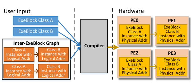
Figure 9 shows the programming model for RISC-NN:
- •
User Inputs, which includes:
- –
Definition of ExeBlock Classes. As will be discussed in Section 5.2, a typical RISC-NN task comprises of multiple ExeBlocks with only few identical styles. A programmer needs to first provide the definition of the different ExeBlocks styles (a.k.a., ExeBlock Classes) which, just like ExeBlocks, are composed of RISC-NN instructions. Yet, their operation fields are address parameters instead of hardware physical addresses.
- –
Execution Graph. It consists of the instances of ExeBlocks Classes and the graph defining the relationship of the ExeBlock Instances. In ExeBlock Instances, the address parameters are replaced by logical (hardware irrelevant) addresses. The programmer also needs to assign a logical PE id to each ExeBlock Instance.
Note that, the data sharing is defined in Execution Graph. For example, if the instructions of two ExeBlock Instances will access the same operand data (e.g., 0x07 in ExeBlocks-0&1 of Figure 8), the programmer needs to first assign the same logical PE id to both ExeBlock Instances to make sure the compiler will map them to the same physical PE. Then for the data-sharing instructions, the logical addresses of corresponding operands should be the same.
- –
- •
Translator Responsibility. We use a simple C++-based translator to handle the user inputs and maps them to the RISC-NN hardware. Its responsibility includes:
- –
Mapping ExeBlocks to physical PEs. The compiler optimizes the load-balancing among PE by considering the available resources of different PEs (i.e., current ExeBlock count, available entries in Instruction/Operand RAM Modules, etc.).
- –
Mapping logical in-PE addresses to physical entries in Operand RAM Module. Here the compiler also balances the occupancy among the banks of each Operand RAM Module to reduce the chance of Operand RAM conflict (Section 3.7).
- –
Mapping logical DRAM addresses to physical DRAM addresses.
- –
4 Experiment Methodology
| Layers/ | Batch | Type | Compress |
|---|---|---|---|
| Operators | Size | Rate | |
| GoogLeNet_CONV1 [46] | 128 | CNN | N/A |
| GoogLeNet_CONV5a_5 [46] | 128 | CNN | N/A |
| VGG16_CONV4 [43] | 64 | CNN | 36% [23] |
| VGG16_CONV9 [43] | 64 | CNN | 27% [23] |
| VGG16_CONV11 [43] | 64 | CNN | 35% [23] |
| AlexNet_CONV2 [31] | 256 | CNN | 38% [23] |
| AlexNet_CONV3 [31] | 256 | CNN | 35% [23] |
| ResNet_CONV2_2 [24] | 64 | CNN | N/A |
| ResNet_CONV3_1 [24] | 64 | CNN | N/A |
| ResNet_CONV4_3 [24] | 64 | CNN | N/A |
| Transformer_ATT [47] | 128 | Attention | N/A |
| Transformer_MMM1 [47] | 128 | MMM | N/A |
| Transformer_MMM2 [47] | 128 | MMM | N/A |
| Transformer_FC1 [47] | 128 | MLP | N/A |
| Transformer_FC2 [47] | 128 | MLP | N/A |
| Sentiment_CNN1 [27] | 500 | 1D CNN | N/A |
| Sentiment_CNN2 [27] | 500 | 1D CNN | N/A |
| Seq2seq_LSTM [12] | 32 | LSTM | N/A |
Table 2 summarizes the parameters of a default RISC-NN system. To evaluate the effectiveness of RISC-NN, we use an in-house cycle-accurate simulator with Ramulator [29] as its memory subsystem. We also implement the design in Verilog and synthesize it using Synopsys Design Compiler with TSMC 12nm GP standard VT library. We then do circuit-level simulations of the atomic operations of RISC-NN using Synopsys VCS and calculate energy consumption using PrimeTime PX. For host data transaction, we use the power consumption of PCIE 3.1[4]. Finally, we feed these energy data back into the simulator to estimate the overall energy consumption of the applications.
As is shown in Table 3, we measure the performance of RISC-NN using layers/operators of multiple NN inference applications, including classical CNN models (GoogLeNet[46], AlexNet[31] and VGG16[43]) and other NN models (ResNet50[24], Transformer[47], a sentiment analysis model based CNN[27]) and seq2Seq[12] from MLPerf [1]. Table 3 shows the detail of these NN benchmarks. Table 3 also shows the compress rates of AlexNet and VGG16 layers [23], as we will use these layers as examples to show effectiveness of RISC-NN for Sparse NN applications.
We compare energy consumption of RISC-NN with state-of-the-art NVIDIA Titan Xp GPGPU [3]. To get accurate energy consumption of each NN layer/operator, we use Caffe2 time [8] or Tensorflow timeline [5] to get execution time, and measure power consumption using Nvidia-smi [2]. Finally, GPGPU energy consumption is product of the measured execution time and power consumption.
5 Experiment Results
5.1 Implementing ISAs of CISC NN Accelerators in RISC-NN
| TPU [28] | Cambricon [33] | |
| Implementable | Read_Host_Memory, | VLOAD, VSTORE, MLOAD |
| Read_Weights, | MSTORE, MMV, VMM | |
| MatrixMultiply, | MMC, OP, MAM, MSM, | |
| Convolve, | VAV, VAS, VMV, VSV, | |
| Activate (simple), | VGTM, VGT, VE, VAND, | |
| VOR, VNOT, SC, SL | ||
| Unnecessary | Activate (complex) | jump, cond. branch, |
| VEXP, VDV, VLOG, RV |
| Size | LD | CAL | COPY | ST | Exe- | OP | |
| Insts | Insts | Insts | Insts | Blocks | RAM | ||
| Entries | |||||||
| MMM | 64x64 | 192 | 4096 | 4928 | 4096 | 255 | 5120 |
| MMV | 64x64 | 4160 | 4096 | 525 | 64 | 255 | 8256 |
| MMS | 64x64 | 4160 | 4096 | 0 | 4096 | 64 | 8256 |
| MAM | 64x64 | 8192 | 4096 | 0 | 4096 | 64 | 12288 |
| OP | 64x64 | 128 | 4096 | 896 | 4096 | 127 | 5120 |
| VGTM | 1024 | 2048 | 1024 | 0 | 1024 | 64 | 3072 |
| VMV | 1024 | 2048 | 1024 | 0 | 1024 | 64 | 3072 |
| LD | CAL | COPY | ST | Exe- | OP | Max | |
| Insts | Insts | Insts | Insts | Blocks | RAM | Inst- | |
| Entries | ances | ||||||
| No | 13056 | 6400 | 0 | 256 | 64 | 13056 | 8 |
| Reuse | |||||||
| Conv | 2976 | 6400 | 15200 | 256 | 256 | 13056 | 8 |
| Reuse | |||||||
| Filter | 6681 | 6400 | 1575 | 256 | 120 | 8256 | 8 |
| Reuse | |||||||
| Ifmap | 6681 | 6400 | 1575 | 256 | 120 | 8256 | 8 |
| Reuse | |||||||
| All | 1136 | 6400 | 8400 | 256 | 254 | 8256 | 8 |
| Reuse |
| Layers | No | Conv | Filter | Ifmap | All |
| Reuse | Reuse | Reuse | Reuse | Reuse | |
| GoogLeNet_CONV1 | 3 | 4 | 7 | 6 | 6 |
| GoogLeNet_CONV- | 4 | 4 | 7 | 8 | 8 |
| -5a_5 | |||||
| VGG16_CONV4 | 1 | 2 | 1 | 3 | 8 |
| VGG16_CONV9 | 3 | 7 | 3 | 8 | 8 |
| VGG16_CONV11 | 1 | 8 | 1 | 8 | 8 |
| AlexNet_CONV2 | 3 | 6 | 4 | 8 | 8 |
| AlexNet_CONV3 | 4 | 6 | 5 | 8 | 8 |
| ResNet_CONV2_2 | 1 | 3 | 2 | 6 | 8 |
| Average | 2.5 | 5 | 3.75 | 6.88 | 7.75 |
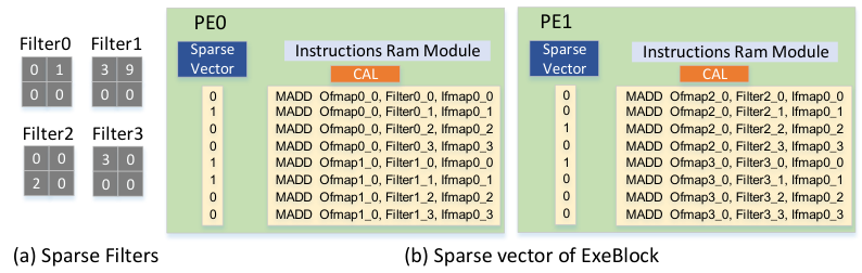


Table 4 summarizes the implementability of all the CISC instructions of TPU [28] and Cambricon [33] on RISC-NN. We can see the following:
- •
RISC-NN can implement most of these instructions.
- •
RISC-NN can achieve the same behavior of two control instructions (i.e., jump and conditional branch) through inter-task management (either through host or control interface). Therefore these two instructions are not necessary for RISC-NN.
- •
Five CISC instructions (complex activate, VEXP, VDV, VLOG and RV), which are mainly used for complex activation functions and classifiers, are unimplementable with RISC-NN ISAs. Instead, as is discussed in Section 3.9, RISC-NN uses an alternate solution which implements these functions as In-DRAM lookup tables.
Table 5 shows the implementation details of several Cambricon [33] CISC instructions on RISC-NN. We can see that, all these implementations have quite a high ratio of memory instructions (LD and ST) to CAL instructions. As we will show in Section 5.2, this phenomenon indicates that these instructions have poor data reuse within the PE array and thus are not well optimized.
We acknowledge RISC-NN has a higher code size overhead than CISC accelerators [38, 36, 28, 33]. However, as will be shown in the rest of the section, the benefits of RISC clearly outweigh its code size overhead. Additionally, such overhead can be largely offset by two countermeasures: (1) When RISC-NN executes the same application for multiple times (common case for cloud-based NN accelerators [28]), the instructions need to be loaded only once and reused thereafter; (2) Using SIMD also effectively offsets the overhead by sharing a single instruction on multiple data points.
5.2 Optimizing CNN in RISC-NN
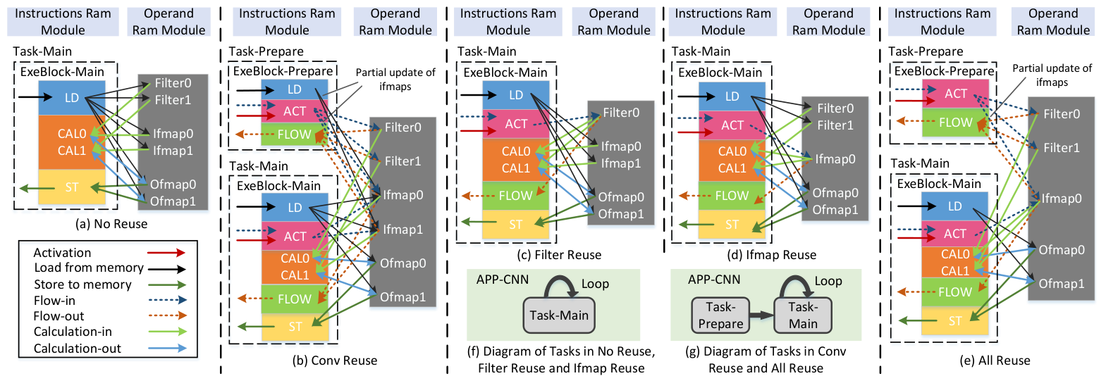
To show the flexibility and programmability of RISC-NN, we analyze in detail of some typical CNN 2D convolution layers (see Table 3). As is shown in Figure 10, following the category mechanism proposed by Chen et al. [16], we evaluate five CNN implementations with different data reuse mechanisms on RISC-NN. No Reuse is the baseline scheme that has no data reuse, while Filter Reuse and Ifmap Reuse reuse the whole filters and input feature map chunks (both at the granularity of 2D filter size), respectively. These three implementations have only one task (i.e., Task-Main), which loops itself multiple times. Meanwhile, Conv Reuse introduces more complex partial inter-PE data sharing of the filters and input feature maps to further reduce off-chip memory traffic. To fulfill such data sharing, Conv Reuse needs the assistance of a single-run preprocess task (i.e., Task-Prepare). All Reuse combines all the aforementioned reuse techniques together. Note that, Conv Reuse and All Reuse, which were implemented in a recent ASIC CNN accelerator [16], cannot be achieved in CISC-NN accelerators [33][28]. This fact indicates that RISC-NN achieves higher programmability than CISC-NN accelerators.
5.2.1 Static Analysis of CNN Implementations.
Table 6 shows the static program statistics of all the CNN implementations of AlexNet_CONV2:
- •
All implementations have the same number of CAL instructions.
- •
No Reuse has the highest number of LD instructions because of its lack of data reuse. Conv Reuse, Filter Reuse and Ifmap Reuse all substantially reduce the number of LD instructions. All Reuse, as the combination of all the reuse schemes, achieves the fewest LD instructions and thus the lightest memory read traffic.
- •
The implementations with reuse mechanisms all use COPY instructions to reuse on-chip data among the ExeBlocks (either intra-PE or inter-PE).
- •
Filter Reuse, Ifmap Reuse and All Reuse also reduce the number of Operand RAM entries used by each task.
As is shown in Table 6, RISC-NN has enough Instruction and Operand RAM Module capacity to incorporate multiple instances of all the CNN implementation (8 in all five CNN implementations of AlexNet_CONV2). Running multiple instances can increase ExeBlock-level parallelism and thus improve the performance. We evaluation the performance impact of running multiple instances in Section 5.2.2.
5.2.2 Performance of CNN Implementations.
Figure 12 shows the performance of RISC-NN in terms of MAC utilization under different CNN implementations with single instance—All Reuse achieves an average MAC unit utilization of 22.91%, remarkably surpassing the results of others (2.12%, 5.21%, 2.30% and 7.96% respectively for No Reuse, Conv Reuse, Filter Reuse and Ifmap Reuse).
Due to conflicts of shared resources, such as NOCs and offchip-Memory, having more instances does not necessarily lead to higher performance. Table 6 shows the instances number of the best MAC unit utilization for five different CNN implementations. The performance of All Reuse keeps increasing as its number of instances increases to about 8; however, this is not the case for other implementations—No Reuse, Conv Reuse, Filter Reuse and Ifmap Reuse achieve their peak performance with an instance number of on average 2.5, 5, 3.75 and 6.88, respectively, and adopting more instances beyond these sweet spots hurts the performance. As is shown in Figure 12, for the multi-instance situation, the best MAC unit utilization of All Reuse (on average 74.43%) is at least more than 2 times higher than the other implementations.
5.2.3 Memory and NoC Traffic of CNN Implementations.
Figures 13 and 14 present the memory and NoC traffic of different CNN implementations with single instance. We can see that, as expected, All Reuse has the least memory traffic—only on average , , and of No Reuse, Conv Reuse, Filter Reuse and Ifmap Reuse, respectively. Note that, Filter Reuse has considerably more memory accesses than Ifmap Reuse because the filters of a CNN application usually have a smaller memory footprint than its input feature maps. This is also the reason why DaDianNao [15] and TPU [28] use large on-chip memories to make input feature maps stay on-chip. Conv Reuse has less memory traffic than Filter Reuse because it also partially reduces the access to off-chip feature maps.
On the NoC traffic side, Memory NoC traffic is proportional to the Off-Chip Memory traffic shown in Figure 13, and the Control NoC traffic takes a quite small portion of all NoC traffic (less than 8% for all implementations). While No Reuse has no Inter-PE NoC traffic since it has no inter-PE data sharing, all the other implementations have a significant amount of Inter-PE traffic to realize their unique inter-PE data-sharing pattern using COPY instructions. An interesting phenomenon is that there is a mismatch of off-chip memory traffic and memory NoC traffic in Ifmap Reuse—compared to All Reuse, Ifmap Reuse has nearly on average 9.39 more Memory NoC traffic but only on average 5.82 more off-chip memory traffic. This happens because the memory request of Ifmap Reuse, the majority of which is input feature map information, achieves a high hit rate (at least 91.92%) in the front-end cache of the memory controller.
5.2.4 Energy Efficiency of CNN Implementations.
Figure 15 shows the normalized energy consumption of all the CNN implementations. We can see that, consistent with NoC and off-chip memory traffic statistics, No Reuse consumes the highest energy while All Reuse consumes the lowest energy.
5.3 Performance Efficiency Over State-of-the-Art GPGPU and CISC NN Accelerator
We compare performance efficiency (in terms of TOPS/W) of RISC-NN with state-of-the-art Nvidia Titan Xp GPGPU and TPU [28].
RISC-NN VS. GPGPU. Since Titan uses 32-bit accuracy instead of 16-bit (the accuracy of RISC-NN implementation), to ensure fair comparison, we also provide extrapolated performance efficiency results of the GPGPU with 16-bit accuracy. As a stream processor, the major part of GPGPU energy is consumed during data movement and such energy is proportional to the number of data moved, therefore we extrapolate that 16-bit accuracy GPGPU has roughly half the energy consumption of its 32-bit counterpart. We can see that, RISC-NN achieves on average 11.88 and 5.94 higher energy performance efficiency over Nvidia Titan Xp with 32-bit and 16-bit accuracy, respectively.
RISC-NN VS. TPU. There were limited performance/power details provided in CISC-NN processors (i.e., Cambricon and TPU). As the best efforts, we compare the average reported MAC unit utilization and performance efficiency of different types of NN applications (i.e., CNN and MLP) in RISC-NN and TPU [28]. As is shown in Figure 17(a), RISC-NN manages to achieve 72.62%, 69.44% and 26.66% MAC unit utilization for CNN, MLP and LSTM; while TPU achieves respectively 54.40% (with high variability), 11.96% and only 3.53% for CNN, MLP and LSTM. This indicates that, compared with CISC NN accelerators, RISC-NN manages to better utilize its hardware resources. As a result of better hardware utilization, RISC-NN also achieves better performance efficiency than TPU with the same 16-bit accuracy—as is shown in Figure 17(b), RISC-NN achieves on average 1.29, 8.37 and 21.71 performance efficiency over TPU for CNN, MLP and LSTM, respectively.
5.4 Sparse NN Optimization
Here we use five Sparse CNN layers [23] as an example to show how RISC-NN takes advantage of the sparsity. As is shown in Figure 19, the compiler first identifies ineffective weights of filters and generates corresponding sparse vector to record the unnecessary instructions in next task. Then, as is discussed in Section 3.4, Instruction Loader takes the sparse vector and translates it into Sparse PC Inc in Instruction RAM. Finally, CAL Unit skips unnecessary instructions according to information of Sparse PC Inc in each instruction.
As is shown in Figure 19, this approach boosts the performance by on average 26.06%, as a result of skipping unnecessary instructions. It also reduces energy consumption by on average 33.13% because of reduction in calculation and accesses to Instruction and Operand RAMs.
5.5 Area Overhead of RISC-NN
The total area of RISC-NN is 14.42, and a single RISC-NN PE takes 0.15. Figure 21 and 21 show the area breakdowns of the whole RISC-NN and a single PE, respectively. We can see that, PE array consumes the majority (67%) of the whole chip area while cache takes only 16%; in the meantime, the area of a single PE is dominated by Operand RAM Module. Such an architecture with small shared cache and large in-PE memory is in line with our design principle of maximizing the data sharing within PEs and reducing transmission overhead of accessing remote data (see Section 3.11).
5.6 Impact of SIMD on Energy Efficiency
Using a high SIMD count in RISC-NN not only reduces the area overhead of the control hardware, but also increase energy efficiency. Figure 22 shows the normalized energy efficiency (in terms of nJ/op) of the All Reuse implementation of AlexNet_CONV2 under different SIMD counts. We can conclude that, the energy overhead of the control hardware diminishes as the SIMD count increases. With SIMD-64, the control energy only takes 0.8% of the total energy consumption. Overall, we can achieve a reasonable control energy overall with SIMD-8.
5.7 Energy Efficiency Scalability
As the number of PE increases in RISC-NN, the energy efficiency of its components should stay largely the same, except for the NOC which on average requires more hops to finish a single request. Without loss of generality, we assume the number of hops and energy consumption per NOC request increase as the square root of PE counts. We then project the energy efficiency of RISC-NN at different scales. As is shown in Figure 23, when running All Reuse applications, the energy efficiency of RISC-NN scales well—even with the extreme scale of 4096 PEs, it energy efficiency is still just 23.1% higher than that of the default 64-PE version, thanks to the optimizations of All Reuse which keeps the data movement minimal.
6 Discussion
| PE Units | RISC-NN | IoT RISC-NN | ||
| config | area () | config | area () | |
| Control Unit | 32 Exeblocks; Unit-Level Concurrency | 3 Exeblocks; No Unit-Level Concurrency | ||
| Calculation Unit | SIMD-8 | SIMD-8 | ||
| Load Unit | default config | default config | ||
| Store Unit | default config | default config | ||
| Flow Unit | default config | default config | ||
| Instruction RAM Module | 8 Banks; Unit-Level Concurrency | 1 Bank; No Unit-Level Concurrency | ||
| Operand RAM Module | 16 Banks; Unit-Level Concurrency | 3 Banks; No Unit-Level Concurrency | ||
| NoC Routers | 128-bit Wide Buffers for Data Routers | 32-bit Wide Buffers for Data Routers | ||
| Total PE Size | ||||
6.1 Use Scenarios for RISC-NN
Currently RISC-NN can be used either as a library-based NN accelerator or as an energy-efficient alternative to FPGA-based NN accelerator, but our ultimate goal is to make it an automatic end platform for high-level NN frameworks:
- •
As a Library-Based NN Accelerator. As is discussed in Section 3.12, the current version of RISC-NN uses a semi-automatic programming model which still needs some effort from programmers to generate performance and energy efficient implementations. Though not ideal, this is an acceptable overhead given the fact that only a few NN applications will be used by a certain customer and applications themselves are not changed frequently. As a result, RISC-NN service providers can develop libraries of typical NN applications for end users to use. Such library-based use scenarios are widely adopted in NN accelerators [28, 20, 21] and proven to be successful.
- •
As an Energy Efficient Alternative to FPGA-based NN Accelerators. In previous sections, we proves that RISC-NN has achieved high flexibility in NN optimization implementation, similar to FPGA-based approaches. Meanwhile, RISC-NN can achieve significantly better energy efficiency, making it an energy efficient alternative to FPGA-based approaches.
- •
As an Automatic End Platform for High-Level NN Framework. Our future work is to develop a compiler to automatically translate the codes of high-level NN frameworks (e.g., PyTorch and Tensorflow) into optimized instructions for RISC-NN. Given the static nature of NN applications and the rich prior research of RISC compiler optimizations, we believe such a goal is achievable.
6.2 Hardware Design Space Exploration
Though RISC-NN is mainly designed to support cloud-based NN acceleration which has a strict performance and energy efficiency requirement, we believe it can also fit into other markets with some design adaptions.
Without loss of generality, we discuss how to adapt RISC-NN to fit the requirements of IoT (Internet-of-Things) NN applications, which have a strict power/area budget to meet the target performance. Table 8 shows the details of such an adaption (i.e., IoT RISC-NN). Compared with RISC-NN, IoT RISC-NN manages to achieve similar energy efficiency but reduce 78.6% of the PE area by slashing the number of RAM banks, router buffer depth and concurrency. This comes at a cost of reduction in available performance–IoT RISC-NN only achieves 7% of MAC Unit Utilization with AlexNet_CONV2 compared with 81% in RISC-NN. Yet, IoT RISC-NN still achieves a performance of 135.2GOPS which is well above the performance requirements of typical IoT NN applications.
7 Conclusions
We believe RISC is a better design choice for NN accelerators over CISC. To prove our concept, we propose a many-core RISC NN accelerator (i.e., RISC-NN) with a 11-instruction Very-RISC ISA and other carefully selected design solutions such as distributed control, dataflow and SIMD.
We show that RISC-NN can realize all the necessary instructions of state-of-the-art CISC NN Accelerators [33, 28]. As proof of its superior programmability, our experiments show that RISC-NN can realize the advanced CNN optimizations and optimization for Sparse NN, both of which previously were only available in ASIC NN Accelerators [16][50]. For a variety of NN applications, RISC-NN achieves on average 11.88 performance efficiency over state-of-the-art Nvidia Titan Xp GPGPU. It also achieves on average 1.29, 8.37 and 21.71 performance efficiency over CISC-based TPU in CNN, MLP and LSTM applications. Finally, by applying pruning optimization, RISC-NN achieves additional on average 26.06% performance improvement and 33.13% energy reduction for Sparse NN applications.
References
- [1] mlperf. https://mlperf.org.
- [2] Nvidia-smi. https://developer.nvidia.com/nvidia-system-management-interface.
- [3] NVIDIA Titan Xp. https://www.nvidia.com/en-us/titan/titan-xp/.
- [4] Power gating: Reducing pci express power consumption to mobile levels.
- [5] TensorFlow. https://www.tensorflow.org/.
- [6] Connection autonomy in simd computers: A vlsi implementation. Journal of Parallel and Distributed Computing, 7(2):302 – 320, 1989.
- [7] Measuring advertisement effectiveness—a neural network approach. Expert Systems with Applications, 31(1):159 – 163, 2006.
- [8] Caffe: Convolutional Architecture for Fast Feature Embedding. In Proceedings of the 22Nd ACM International Conference on Multimedia, MM ’14, New York, NY, USA, 2014.
- [9] General-purpose computing on graphics processing units. Wikipedia, Feb. 2018. Page Version ID: 824446103.
- [10] J. Albericio, P. Judd, T. Hetherington, T. Aamodt, N. E. Jerger, and A. Moshovos. Cnvlutin: ineffectual-neuron-free deep neural network computing. In Computer Architecture (ISCA), 2016 ACM/IEEE 43rd Annual International Symposium on, pages 1–13. IEEE, 2016.
- [11] M. Bojarski, D. D. Testa, D. Dworakowski, B. Firner, B. Flepp, P. Goyal, L. D. Jackel, M. Monfort, U. Muller, J. Zhang, X. Zhang, J. Zhao, and K. Zieba. End to end learning for self-driving cars. CoRR, abs/1604.07316, 2016.
- [12] D. Britz, A. Goldie, T. Luong, and Q. Le. Massive Exploration of Neural Machine Translation Architectures. ArXiv e-prints, Mar. 2017.
- [13] R. Cai, A. Ren, N. Liu, C. Ding, L. Wang, X. Qian, M. Pedram, and Y. Wang. Vibnn: Hardware acceleration of bayesian neural networks. In Proceedings of the Twenty-Third International Conference on Architectural Support for Programming Languages and Operating Systems, ASPLOS ’18, pages 476–488, 2018.
- [14] T. Chen, Z. Du, N. Sun, J. Wang, C. Wu, Y. Chen, and O. Temam. Diannao: A small-footprint high-throughput accelerator for ubiquitous machine-learning. In ACM Sigplan Notices, pages 269–284. ACM, 2014.
- [15] Y. Chen, T. Luo, S. Liu, S. Zhang, L. He, J. Wang, L. Li, T. Chen, Z. Xu, N. Sun, and O. Temam. Dadiannao: A machine-learning supercomputer. In Proceedings of the 47th Annual IEEE/ACM International Symposium on Microarchitecture, MICRO-47, pages 609–622, 2014.
- [16] Y.-H. Chen, J. Emer, and V. Sze. Eyeriss: A spatial architecture for energy-efficient dataflow for convolutional neural networks. In ACM SIGARCH Computer Architecture News, volume 44, pages 367–379. IEEE Press, 2016.
- [17] C. Deng, S. Liao, Y. Xie, K. K. Parhi, X. Qian, and B. Yuan. Permdnn: Efficient compressed dnn architecture with permuted diagonal matrices. In 2018 51st Annual IEEE/ACM International Symposium on Microarchitecture (MICRO), pages 189–202, 2018.
- [18] C. Deng, F. Sun, X. Qian, J. Lin, Z. Wang, and B. Yuan. Tie: Energy-efficient tensor train-based inference engine for deep neural network. In Proceedings of the 46th International Symposium on Computer Architecture, pages 264–278, 2019.
- [19] C. Farabet, B. Martini, B. Corda, P. Akselrod, E. Culurciello, and Y. LeCun. NeuFlow: A runtime reconfigurable dataflow processor for vision. In CVPR 2011 WORKSHOPS, pages 109–116, 2011.
- [20] E. Flamand, D. Rossi, F. Conti, I. Loi, A. Pullini, F. Rotenberg, and L. Benini. Gap-8: A risc-v soc for ai at the edge of the iot. In 2018 IEEE 29th International Conference on Application-specific Systems, Architectures and Processors (ASAP), pages 1–4, 2018.
- [21] A. Garofalo, M. Rusci, F. Conti, D. Rossi, and L. Benini. Pulp-nn: A computing library for quantized neural network inference at the edge on risc-v based parallel ultra low power clusters. In 2019 26th IEEE International Conference on Electronics, Circuits and Systems (ICECS), pages 33–36, 2019.
- [22] S. Han, X. Liu, H. Mao, J. Pu, A. Pedram, M. A. Horowitz, and W. J. Dally. Eie: efficient inference engine on compressed deep neural network. In Proceedings of the 43rd International Symposium on Computer Architecture, pages 243–254, 2016.
- [23] S. Han, H. Mao, and W. J. Dally. Deep Compression: Compressing Deep Neural Networks with Pruning, Trained Quantization and Huffman Coding. arXiv e-prints, Oct. 2015.
- [24] K. He, X. Zhang, S. Ren, and J. Sun. Delving deep into rectifiers: Surpassing human-level performance on imagenet classification. In 2015 IEEE International Conference on Computer Vision (ICCV), pages 1026–1034, Dec 2015.
- [25] K. Hegde, J. Yu, R. Agrawal, M. Yan, M. Pellauer, and C. Fletcher. Ucnn: Exploiting computational reuse in deep neural networks via weight repetition. In 2018 ACM/IEEE 45th Annual International Symposium on Computer Architecture (ISCA), pages 674–687, 2018.
- [26] G. Hinton, L. Deng, D. Yu, G. E. Dahl, A. r. Mohamed, N. Jaitly, A. Senior, V. Vanhoucke, P. Nguyen, T. N. Sainath, and B. Kingsbury. Deep neural networks for acoustic modeling in speech recognition: The shared views of four research groups. IEEE Signal Processing Magazine, 29(6):82–97, Nov 2012.
- [27] R. Johnson and T. Zhang. Effective use of word order for text categorization with convolutional neural networks. CoRR, abs/1412.1058, 2014.
- [28] N. P. Jouppi, C. Young, N. Patil, D. Patterson, G. Agrawal, R. Bajwa, S. Bates, S. Bhatia, N. Boden, A. Borchers, R. Boyle, P.-l. Cantin, C. Chao, C. Clark, J. Coriell, M. Daley, M. Dau, J. Dean, B. Gelb, T. V. Ghaemmaghami, R. Gottipati, W. Gulland, R. Hagmann, C. R. Ho, D. Hogberg, J. Hu, R. Hundt, D. Hurt, J. Ibarz, A. Jaffey, A. Jaworski, A. Kaplan, H. Khaitan, D. Killebrew, A. Koch, N. Kumar, S. Lacy, J. Laudon, J. Law, D. Le, C. Leary, Z. Liu, K. Lucke, A. Lundin, G. MacKean, A. Maggiore, M. Mahony, K. Miller, R. Nagarajan, R. Narayanaswami, R. Ni, K. Nix, T. Norrie, M. Omernick, N. Penukonda, A. Phelps, J. Ross, M. Ross, A. Salek, E. Samadiani, C. Severn, G. Sizikov, M. Snelham, J. Souter, D. Steinberg, A. Swing, M. Tan, G. Thorson, B. Tian, H. Toma, E. Tuttle, V. Vasudevan, R. Walter, W. Wang, E. Wilcox, and D. H. Yoon. In-datacenter performance analysis of a tensor processing unit. In Proceedings of the 44th Annual International Symposium on Computer Architecture, ISCA ’17, pages 1–12, 2017.
- [29] Y. Kim, W. Yang, and O. Mutlu. Ramulator: A fast and extensible dram simulator. IEEE Computer Architecture Letters, 15(1):45–49, Jan 2016.
- [30] A. Krizhevsky, I. Sutskever, and G. E. Hinton. Imagenet classification with deep convolutional neural networks. In F. Pereira, C. J. C. Burges, L. Bottou, and K. Q. Weinberger, editors, Advances in Neural Information Processing Systems 25, pages 1097–1105. 2012.
- [31] A. Krizhevsky, I. Sutskever, and G. E. Hinton. ImageNet Classification with Deep Convolutional Neural Networks. In F. Pereira, C. J. C. Burges, L. Bottou, and K. Q. Weinberger, editors, Advances in Neural Information Processing Systems 25, pages 1097–1105. Curran Associates, Inc., 2012.
- [32] H. Kwon, A. Samajdar, and T. Krishna. Maeri: Enabling flexible dataflow mapping over dnn accelerators via reconfigurable interconnects. In Proceedings of the Twenty-Third International Conference on Architectural Support for Programming Languages and Operating Systems, ASPLOS ’18, pages 461–475, 2018.
- [33] S. Liu, Z. Du, J. Tao, D. Han, T. Luo, Y. Xie, Y. Chen, and T. Chen. Cambricon: An Instruction Set Architecture for Neural Networks. In 2016 ACM/IEEE 43rd Annual International Symposium on Computer Architecture (ISCA), pages 393–405, 2016.
- [34] W. Lu, G. Yan, J. Li, S. Gong, Y. Han, and X. Li. FlexFlow: A Flexible Dataflow Accelerator Architecture for Convolutional Neural Networks. In 2017 IEEE International Symposium on High Performance Computer Architecture (HPCA), pages 553–564, 2017.
- [35] M. Mahmoud, K. Siu, and A. Moshovos. Diffy: a déjà vu-free differential deep neural network accelerator. In 2018 51st Annual IEEE/ACM International Symposium on Microarchitecture (MICRO), pages 134–147, 2018.
- [36] T. Nowatzki, V. Gangadhar, N. Ardalani, and K. Sankaralingam. Stream-dataflow acceleration. In 2017 ACM/IEEE 44th Annual International Symposium on Computer Architecture (ISCA), pages 416–429, 2017.
- [37] E. Park, D. Kim, and S. Yoo. Energy-efficient neural network accelerator based on outlier-aware low-precision computation. In 2018 ACM/IEEE 45th Annual International Symposium on Computer Architecture (ISCA), pages 688–698, 2018.
- [38] R. Prabhakar, Y. Zhang, D. Koeplinger, M. Feldman, T. Zhao, S. Hadjis, A. Pedram, C. Kozyrakis, and K. Olukotun. Plasticine: A reconfigurable architecture for parallel patterns. In 2017 ACM/IEEE 44th Annual International Symposium on Computer Architecture (ISCA), pages 389–402, 2017.
- [39] B. Reagen, P. Whatmough, R. Adolf, S. Rama, H. Lee, S. K. Lee, J. M. Hernández-Lobato, G.-Y. Wei, and D. Brooks. Minerva: Enabling low-power, highly-accurate deep neural network accelerators. In Proceedings of the 43rd International Symposium on Computer Architecture, pages 267–278. IEEE Press, 2016.
- [40] A. Shafiee, A. Nag, N. Muralimanohar, R. Balasubramonian, J. P. Strachan, M. Hu, R. S. Williams, and V. Srikumar. Isaac: A convolutional neural network accelerator with in-situ analog arithmetic in crossbars. In Proc. ISCA, 2016.
- [41] S. Sharify, A. D. Lascorz, M. Mahmoud, M. Nikolic, K. Siu, D. M. Stuart, Z. Poulos, and A. Moshovos. Laconic deep learning inference acceleration. In Proceedings of the 46th International Symposium on Computer Architecture, pages 304–317, 2019.
- [42] Y. Shen, M. Ferdman, and M. Peter. Maximizing cnn accelerator efficiency through resource partitioning. In Proceedings of the 44th Annual International Symposium on Computer Architecture, pages 535–547. ACM, 2017.
- [43] K. Simonyan and A. Zisserman. Very deep convolutional networks for large-scale image recognition. Computer Science, 2014.
- [44] L. Song, Y. Wang, Y. Han, X. Zhao, B. Liu, and X. Li. C-brain: A deep learning accelerator that tames the diversity of cnns through adaptive data-level parallelization. In 2016 53nd ACM/EDAC/IEEE Design Automation Conference (DAC), pages 1–6, 2016.
- [45] M. Song, J. Zhang, H. Chen, and T. Li. Towards efficient microarchitectural design for accelerating unsupervised gan-based deep learning. In 2018 IEEE International Symposium on High Performance Computer Architecture (HPCA), pages 66–77, 2018.
- [46] C. Szegedy, Wei Liu, Yangqing Jia, P. Sermanet, S. Reed, D. Anguelov, D. Erhan, V. Vanhoucke, and A. Rabinovich. Going deeper with convolutions. In 2015 IEEE Conference on Computer Vision and Pattern Recognition (CVPR), pages 1–9, June 2015.
- [47] A. Vaswani, N. Shazeer, N. Parmar, J. Uszkoreit, L. Jones, A. N. Gomez, L. Kaiser, and I. Polosukhin. Attention is all you need. CoRR, abs/1706.03762, 2017.
- [48] S. Venkataramani, A. Ranjan, S. Banerjee, D. Das, S. Avancha, A. Jagannathan, A. Durg, D. Nagaraj, B. Kaul, P. Dubey, and A. Raghunathan. Scaledeep: A scalable compute architecture for learning and evaluating deep networks. In Proceedings of the 44th Annual International Symposium on Computer Architecture, pages 13–26. ACM, 2017.
- [49] D. Voitsechov and Y. Etsion. Single-graph multiple flows: Energy efficient design alternative for gpgpus. In Proceeding of the 41st Annual International Symposium on Computer Architecuture, ISCA ’14, pages 205–216, 2014.
- [50] S. Zhang, Z. Du, L. Zhang, H. Lan, S. Liu, L. Li, Q. Guo, T. Chen, and Y. Chen. Cambricon-X: An accelerator for sparse neural networks. In 2016 49th Annual IEEE/ACM International Symposium on Microarchitecture (MICRO), pages 1–12, 2016.