跳到论文正文
W Papers独立论文阅读器 arXiv:2103.12392 论文正文 计算阅读时间 · 0%
引用这篇论文根据当前论文元数据生成,正式投稿前建议核对。


License: CC BY-SA 4.0
arXiv:2103.12392v2 [math.AP] 14 Dec 2022

A mathematical analysis of the Kakinuma model
for interfacial gravity waves.
Part I: Structures and well-posedness

Vincent Duchêne and Tatsuo Iguchi

Abstract

We consider a model, which we named the Kakinuma model, for interfacial gravity waves. As is well-known, the full model for interfacial gravity waves has a variational structure whose Lagrangian is an extension of Luke’s Lagrangian for surface gravity waves, that is, water waves. The Kakinuma model is a system of Euler–Lagrange equations for approximate Lagrangians, which are obtained by approximating the velocity potentials in the Lagrangian for the full model. In this paper, we first analyze the linear dispersion relation for the Kakinuma model and show that the dispersion curves highly fit that of the full model in the shallow water regime. We then analyze the linearized equations around constant states and derive a stability condition, which is satisfied for small initial data when the denser water is below the lighter water. We show that the initial value problem is in fact well-posed locally in time in Sobolev spaces under the stability condition, the non-cavitation assumption and intrinsic compatibility conditions in spite of the fact that the initial value problem for the full model does not have any stability domain so that its initial value problem is ill-posed in Sobolev spaces. Moreover, it is shown that the Kakinuma model enjoys a Hamiltonian structure and has conservative quantities: mass, total energy, and in the case of the flat bottom, momentum.

1 Introduction

We are concerned with the motion of interfacial gravity waves at the interface between two layers of immiscible waters in a domain of the (n+1)(n+1)-dimensional Euclidean space in the rigid-lid case. Let tt be the time, 𝒙=(x1,…,xn)\bm{x}=(x_{1},\ldots,x_{n}) the horizontal spatial coordinates, and zz the vertical spatial coordinate. We assume that the interface, the rigid-lid of the upper layer, and the bottom of the lower layer are represented as z=ζ⁡(𝒙,t)z=\zeta(\bm{x},t), z=h1z=h_{1}, and z=−h2+b⁡(𝒙)z=-h_{2}+b(\bm{x}), respectively, where ζ⁡(𝒙,t)\zeta(\bm{x},t) is the elevation of the interface, h1h_{1} and h2h_{2} are mean thicknesses of the upper and lower layers, and b⁡(𝒙)b(\bm{x}) represents the bottom topography. The only external force applied to the system is the constant and vertical gravity, and interfacial tension is neglected. Moreover, we assume that the waters in the upper and the lower layers are both incompressible and inviscid fluids with constant densities ρ1\rho_{1} and ρ2\rho_{2}, respectively, and that the flows are both irrotational. See Figure 1.1.
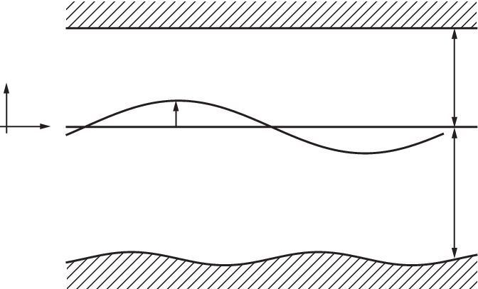
Refer to caption
Figure 1.1: Interfacial gravity waves

Then, the motion of the waters is described by the velocity potentials Φ1\Phi_{1} and Φ2\Phi_{2} and the pressures P1P_{1} and P2P_{2} in the upper and the lower layers, respectively, satisfying the basic equations in the theory of fluid dynamics, which will be referred as the full model for interfacial gravity waves throughout in this paper. As shown by J. C. Luke [23], the basic equations for the surface gravity waves, that is, the water wave problem has a variational structure, whose Lagrangian is written in terms of the surface elevation of the water and the velocity potential, and the Lagrangian density is given by the vertical integral of the pressure in the water region. The full model for interfacial gravity waves has also a variational structure and the Lagrangian density ℒ⁡(Φ1,Φ2,ζ)\mathscr{L}(\Phi_{1},\Phi_{2},\zeta) is again given by the vertical integral of the pressure in both water regions. T. Kakinuma [17, 18, 19] proposed a model for interfacial gravity waves and applied his model to simulate numerically the waves. To derive the model, he approximated the velocity potentials Φ1\Phi_{1} and Φ2\Phi_{2} by

(1.1) Φkapp​(𝒙,z,t)=∑i=0NZk,i​(z,h~k​(𝒙))​ϕk,i​(𝒙,t)\Phi_{k}^{\rm app}(\bm{x},z,t)=\sum_{i=0}^{N}Z_{k,i}(z;\tilde{h}_{k}(\bm{x}))\phi_{k,i}(\bm{x},t)

for k=1,2k=1,2, where {Z1,i}\{Z_{1,i}\} and {Z2,i}\{Z_{2,i}\} are appropriate function systems in the vertical coordinate zz and may depend on h~1​(𝒙)\tilde{h}_{1}(\bm{x}) and h~2​(𝒙)\tilde{h}_{2}(\bm{x}), respectively, which are thickness of the upper and the lower layers in the rest state, whereas ϕk=(ϕk,0,ϕk,1,…,ϕk,N)T\bm{\phi}_{k}=(\phi_{k,0},\phi_{k,1},\ldots,\phi_{k,N})^{\rm T}, k=1,2k=1,2, are unknown variables. Then, he derived an approximate Lagrangian density ℒapp​(ϕ1,ϕ2,ζ)=ℒ⁡(Φ1app,Φ2app,ζ)\mathscr{L}^{\rm app}(\bm{\phi}_{1},\bm{\phi}_{2},\zeta)=\mathscr{L}(\Phi_{1}^{\rm app},\Phi_{2}^{\rm app},\zeta) for unknowns (ϕ1,ϕ2,ζ)(\bm{\phi}_{1},\bm{\phi}_{2},\zeta). The Kakinuma model is a corresponding system of Euler–Lagrange equations for the approximated Lagrangian density ℒapp​(ϕ1,ϕ2,ζ)\mathscr{L}^{\rm app}(\bm{\phi}_{1},\bm{\phi}_{2},\zeta). Different choices of the function systems {Z1,i}\{Z_{1,i}\} and {Z2,i}\{Z_{2,i}\} give different Kakinuma models and we have to carefully choose the function systems for the Kakinuma model to provide good approximations for interfacial gravity waves.

The Kakinuma model is an extension to interfacial gravity waves of the so-called Isobe–Kakinuma model for the surface gravity waves, that is, the water waves. In the case of the surface gravity waves, the basic equations are known to have a variational structure with Luke’s Lagrangian density ℒLuke​(Φ,ζ)\mathscr{L}_{\rm Luke}(\Phi,\zeta), where ζ\zeta is the surface elevation and Φ\Phi is the velocity potential of the water. The Isobe–Kakinuma model is a system of Euler–Lagrange equations for the approximated Lagrangian density ℒapp​(ϕ,ζ)=ℒLuke​(Φapp,ζ)\mathscr{L}^{\rm app}(\bm{\phi},\zeta)=\mathscr{L}_{\rm Luke}(\Phi^{\rm app},\zeta), where Φapp\Phi^{\rm app} is an approximate velocity potential

(1.2) Φapp​(𝒙,z,t)=∑i=0NZi​(z,b⁡(𝒙))​ϕi​(𝒙,t)\Phi^{\rm app}(\bm{x},z,t)=\sum_{i=0}^{N}Z_{i}(z;b(\bm{x}))\phi_{i}(\bm{x},t)

and ϕ=(ϕ0,ϕ1,…,ϕN)T\bm{\phi}=(\phi_{0},\phi_{1},\ldots,\phi_{N})^{\rm T} are unknown variables. The model was first proposed by M. Isobe [15, 16] and then applied by T. Kakinuma to simulate numerically the water waves. We note that a similar model was derived by G. Klopman, B. van Groesen, and M. W. Dingemans [21], and used to simulate the water waves. See also Ch. E. Papoutsellis and G. A. Athanassoulis [29]. Recently, this model was analyzed from mathematical point of view. One possible choice of the function system {Zi}\{Z_{i}\} is a set of polynomials in zz, for example, Zi​(z,b⁡(𝒙))=(z+h−b⁡(𝒙))piZ_{i}(z;b(\bm{x}))=(z+h-b(\bm{x}))^{p_{i}} with integers pip_{i} satisfying 0=p0<p1<⋯<pN0=p_{0}<p_{1}<\cdots<p_{N}. Under this choice of the function system {Zi}\{Z_{i}\}, the initial value problem to the Isobe–Kakinuma model was analyzed by Y. Murakami and T. Iguchi [27] in a special case and by R. Nemoto and T. Iguchi [28] in the general case. The hypersurface t=0t=0 in the space-time 𝐑n×𝐑\mathbf{R}^{n}\times\mathbf{R} is characteristic for the Isobe–Kakinuma model, so that one needs to impose some compatibility conditions on the initial data for the existence of the solution. Under these compatibility conditions and a sign condition −∂zPapp≥c0>0-\partial_{z}P^{\rm app}\geq c_{0}>0 on the water surface, they showed the well-posedness of the initial value problem locally in time, where PappP^{\rm app} is an approximate pressure in the Isobe–Kakinuma model calculated from Bernoulli’s equation. Moreover, T. Iguchi [12, 13] showed that under the choice of the function system

(1.3) Zi​(z,b⁡(𝒙))={(z+h)2​iin the case of the flat bottom,(z+h−b⁡(𝒙))iin the case of a variable bottom,Z_{i}(z;b(\bm{x}))=\begin{cases}(z+h)^{2i}&\mbox{in the case of the flat bottom},\\ (z+h-b(\bm{x}))^{i}&\mbox{in the case of a variable bottom},\end{cases}

the Isobe–Kakinuma model is a higher order shallow water approximation for the water wave problem in the strongly nonlinear regime. Furthermore, V. Duchêne and T. Iguchi [8] showed that the Isobe–Kakinuma model also enjoys a Hamiltonian structure analogous to the one exhibited by V. E. Zakharov [32] on the full water wave problem. Our aim in the present paper is to extend these results on the surface gravity waves to interfacial gravity waves.

In view of these results on the Isobe–Kakinuma model, in the present paper we consider the Kakinuma model under the choice of the approximate velocity potentials in (1.1) as

(1.4) {Φ1app​(𝒙,z,t)=∑i=0N(−z+h1)2​i​ϕ1,i​(𝒙,t),Φ2app​(𝒙,z,t)=∑i=0N∗(z+h2−b⁡(𝒙))pi​ϕ2,i​(𝒙,t),\begin{cases}\displaystyle\Phi_{1}^{\rm app}(\bm{x},z,t)=\sum_{i=0}^{N}(-z+h_{1})^{2i}\phi_{1,i}(\bm{x},t),\\[10.76385pt] \displaystyle\Phi_{2}^{\rm app}(\bm{x},z,t)=\sum_{i=0}^{N^{*}}(z+h_{2}-b(\bm{x}))^{p_{i}}\phi_{2,i}(\bm{x},t),\end{cases}

where N,N∗N,N^{*} and p0,p1,…,pN∗p_{0},p_{1},\ldots,p_{N^{*}} are nonnegative integers satisfying 0=p0<p1<⋯<pN∗0=p_{0}<p_{1}<\cdots<p_{N^{*}}. In applications of the Kakinuma model, it would be better to choose N∗=NN^{*}=N and pi=2​ip_{i}=2i in the case of the flat bottom, and N∗=2​NN^{*}=2N and pi=ip_{i}=i in the case of a variable bottom. In the case N=N∗=0N=N^{*}=0, that is, if we choose the approximation Φkapp​(𝒙,z,t)=ϕk​(𝒙,t)\Phi_{k}^{\rm app}(\bm{x},z,t)=\phi_{k}(\bm{x},t) for k=1,2k=1,2 the functions independent of the vertical coordinate zz, then the corresponding Kakinuma model is reduced to the shallow water equations. In the case N+N∗>0N+N^{*}>0, the Kakinuma model is classified into a system of nonlinear dispersive equations.

It is well-known that in the case of the flat bottom b=0b=0, the dispersion relation of the linearized equations to the full model around the flow (ζ,Φ1,Φ2)=(0,𝒖1⋅𝒙,𝒖2⋅𝒙)(\zeta,\Phi_{1},\Phi_{2})=(0,\bm{u}_{1}\cdot\bm{x},\bm{u}_{2}\cdot\bm{x}) with constant horizontal velocities 𝒖1\bm{u}_{1} and 𝒖2\bm{u}_{2} is given by

(ρ1​coth⁡(h1​|𝝃|)+ρ2​coth⁡(h2​|𝝃|))​ω2\displaystyle(\rho_{1}\coth(h_{1}|\bm{\xi}|)+\rho_{2}\coth(h_{2}|\bm{\xi}|))\omega^{2}
+2​(ρ1​𝝃⋅𝒖1​coth⁡(h1​|𝝃|)+ρ2​𝝃⋅𝒖2​coth⁡(h2​|𝝃|))​ω\displaystyle+2(\rho_{1}\bm{\xi}\cdot\bm{u}_{1}\coth(h_{1}|\bm{\xi}|)+\rho_{2}\bm{\xi}\cdot\bm{u}_{2}\coth(h_{2}|\bm{\xi}|))\omega
+ρ1​(𝝃⋅𝒖1)2​coth⁡(h1​|𝝃|)+ρ2​(𝝃⋅𝒖2)2​coth⁡(h2​|𝝃|)−(ρ2−ρ1)​g​|𝝃|=0,\displaystyle+\rho_{1}(\bm{\xi}\cdot\bm{u}_{1})^{2}\coth(h_{1}|\bm{\xi}|)+\rho_{2}(\bm{\xi}\cdot\bm{u}_{2})^{2}\coth(h_{2}|\bm{\xi}|)-(\rho_{2}-\rho_{1})g|\bm{\xi}|=0,

where 𝝃∈𝐑n\bm{\xi}\in\mathbf{R}^{n} is the wave vector, ω∈𝐂\omega\in\mathbf{C} the angular frequency, and gg the gravitational constant. It is easy to see that the roots ω\omega of the above equation are always real for any wave vector 𝝃∈𝐑n\bm{\xi}\in\mathbf{R}^{n} if and only if 𝒖1=𝒖2\bm{u}_{1}=\bm{u}_{2} and ρ2≥ρ1\rho_{2}\geq\rho_{1}. Otherwise, the roots of the above equation have the form ω=ωr​(|𝝃|)±i​ωi​(|𝝃|)\omega=\omega_{r}(|\bm{\xi}|)\pm\mathrm{i}\omega_{i}(|\bm{\xi}|) satisfying ωi​(|𝝃|)→+∞\omega_{i}(|\bm{\xi}|)\to+\infty as |𝝃|→+∞|\bm{\xi}|\to+\infty, which leads to an instability of the interface. The instabilities in the case ρ2>ρ1\rho_{2}>\rho_{1} and 𝒖1≠𝒖2\bm{u}_{1}\neq\bm{u}_{2} and in the case ρ2<ρ1\rho_{2}<\rho_{1} and 𝒖1=𝒖2\bm{u}_{1}=\bm{u}_{2} are known as the Kelvin–Helmholtz and the Rayleigh–Taylor instabilities, respectively. For more details, see for example P. G. Drazin and W. H. Reid [7]. In the following of this paper, we are interested in the situation where

(ρ2−ρ1)​g>0,(\rho_{2}-\rho_{1})g>0,

that is, the denser water is below the lighter water. In the case 𝒖1=𝒖2=𝟎\bm{u}_{1}=\bm{u}_{2}=\bm{0}, the linear dispersion relation is written simply as

ω2=(ρ2−ρ1)​g​|𝝃|ρ1​coth⁡(h1​|𝝃|)+ρ2​coth⁡(h2​|𝝃|).\omega^{2}=\frac{(\rho_{2}-\rho_{1})g|\bm{\xi}|}{\rho_{1}\coth(h_{1}|\bm{\xi}|)+\rho_{2}\coth(h_{2}|\bm{\xi}|)}.

We denote the right-hand side by ωIW​(𝝃)2\omega_{\mbox{\rm\tiny IW}}(\bm{\xi})^{2}. Then, the phase speed cIW​(𝝃)c_{\mbox{\rm\tiny IW}}(\bm{\xi}) of the plane wave solution related to the wave vector 𝝃\bm{\xi} is given by

(1.5) cIW​(𝝃)=ωIW​(𝝃)|𝝃|=±(ρ2−ρ1)​gρ1​|𝝃|​coth⁡(h1​|𝝃|)+ρ2​|𝝃|​coth⁡(h2​|𝝃|).c_{\mbox{\rm\tiny IW}}(\bm{\xi})=\frac{\omega_{\mbox{\rm\tiny IW}}(\bm{\xi})}{|\bm{\xi}|}=\pm\sqrt{\frac{(\rho_{2}-\rho_{1})g}{\rho_{1}|\bm{\xi}|\coth(h_{1}|\bm{\xi}|)+\rho_{2}|\bm{\xi}|\coth(h_{2}|\bm{\xi}|)}}.

As a shallow water limit h1​|𝝃|,h2​|𝝃|→0h_{1}|\bm{\xi}|,h_{2}|\bm{\xi}|\to 0, we have

(1.6) cIW​(𝝃)≃cSW=±(ρ2−ρ1)​g​h1​h2ρ1​h2+ρ2​h1,c_{\mbox{\rm\tiny IW}}(\bm{\xi})\simeq c_{\mbox{\rm\tiny SW}}=\pm\sqrt{\frac{(\rho_{2}-\rho_{1})gh_{1}h_{2}}{\rho_{1}h_{2}+\rho_{2}h_{1}}},

where cSWc_{\mbox{\rm\tiny SW}} is the phase speed of infinitely long and small interfacial gravity waves. In Section 3, we will analyze the linear dispersion relation of the Kakinuma model and calculate the phase speed cK​(𝝃)c_{\mbox{\rm\tiny K}}(\bm{\xi}) of the plane wave solution related to the wave vector 𝝃\bm{\xi}. Under the choice N∗=NN^{*}=N and pi=2​ip_{i}=2i, or N∗=2​NN^{*}=2N and pi=ip_{i}=i in the approximation (1.4) of the velocity potentials, it turns out that

(1.7) |cIW​(𝝃)2−cK​(𝝃)2|≲(h1​|𝝃|+h2​|𝝃|)4​N+2,|c_{\mbox{\rm\tiny IW}}(\bm{\xi})^{2}-c_{\mbox{\rm\tiny K}}(\bm{\xi})^{2}|\lesssim(h_{1}|\bm{\xi}|+h_{2}|\bm{\xi}|)^{4N+2},

which indicates that the Kakinuma model may be a good approximation of the full model for interfacial gravity waves in the shallow water regime h1​|𝝃|,h2​|𝝃|≪1h_{1}|\bm{\xi}|,h_{2}|\bm{\xi}|\ll 1. We note that Miyata–Choi–Camassa model derived by M. Miyata [26] and W. Choi and R. Camassa [4] is a model for interfacial gravity waves in the strongly nonlinear regime and can be regarded as a generalization of the Green–Naghdi equations for water waves into a two-layer system. Let cMCC​(𝝃)c_{\mbox{\rm\tiny MCC}}(\bm{\xi}) be the phase speed of the plane wave solution related to the wave vector 𝝃\bm{\xi} for the linearized equations of the Miyata–Choi–Camassa model around the rest state. Then, we have

|cIW​(𝝃)2−cMCC​(𝝃)2|≲(h1​|𝝃|+h2​|𝝃|)4,|c_{\mbox{\rm\tiny IW}}(\bm{\xi})^{2}-c_{\mbox{\rm\tiny MCC}}(\bm{\xi})^{2}|\lesssim(h_{1}|\bm{\xi}|+h_{2}|\bm{\xi}|)^{4},

so that the Kakinuma model gives a better approximation of the full model than the Miyata–Choi–Camassa model in the shallow water regime, at least, at the linear level. A rigorous analysis for the consistency of the Kakinuma model in the shallow water regime will be analyzed in the subsequent paper V. Duchêne and T. Iguchi [9]. On the other hand, in the deep water limit we have

limh1​|𝝃|,h2​|𝝃|→∞cK​(𝝃)2>0,\lim_{h_{1}|\bm{\xi}|,h_{2}|\bm{\xi}|\to\infty}c_{\mbox{\rm\tiny K}}(\bm{\xi})^{2}>0,

which is not consistent with the limit of the full model

limh1​|𝝃|,h2​|𝝃|→∞cIW​(𝝃)2=0.\lim_{h_{1}|\bm{\xi}|,h_{2}|\bm{\xi}|\to\infty}c_{\mbox{\rm\tiny IW}}(\bm{\xi})^{2}=0.

We notice that the Miyata–Choi–Camassa model is only apparently consistent with the full model in this deep water limit since

limh1​|𝝃|,h2​|𝝃|→∞cMCC​(𝝃)2=0,\lim_{h_{1}|\bm{\xi}|,h_{2}|\bm{\xi}|\to\infty}c_{\mbox{\rm\tiny MCC}}(\bm{\xi})^{2}=0,

but we note also that

limh1​|𝝃|,h2​|𝝃|→∞cIW​(𝝃)2cMCC​(𝝃)2=∞.\lim_{h_{1}|\bm{\xi}|,h_{2}|\bm{\xi}|\to\infty}\frac{c_{\mbox{\rm\tiny IW}}(\bm{\xi})^{2}}{c_{\mbox{\rm\tiny MCC}}(\bm{\xi})^{2}}=\infty.

We refer to V. Duchêne, S. Israwi, and R. Talhouk [10] for further discussion and the derivation of modified Miyata–Choi–Camassa models having either the same dispersion relation as the full model, or the same behavior as the Kakinuma model in the deep water limit. As we discuss below, thanks to the high-frequency behavior of the linearized equations, and contrarily to both the full model and the Miyata–Choi–Camassa model, the Kakinuma model has a non-trivial stability domain and, as a result, the initial value problem to the Kakinuma model is well-posed locally in time in Sobolev spaces under appropriate assumptions on the initial data.

As we have already seen, the roots ω∈𝐂\omega\in\mathbf{C} of the dispersion relation of the linearized equations of the full model around the rest state are always real, so that the corresponding initial value problem is well-posed. However, as for the nonlinear problem, even if the initial velocity is continuous on the interface, a discontinuity of the velocity in the tangential direction on the interface would be created instantaneously in general, so that the Kelvin–Helmholtz instability appears locally in space. As a result, the initial value problem for the full model turns out to be ill-posed. For more details, we refer to T. Iguchi, N. Tanaka, and A. Tani [14]. See also V. Kamotski and G. Lebeau [20] and D. Lannes [22]. In Section 4 we consider the linearized equations of the Kakinuma model around an arbitrary flow. After freezing the coefficients and neglecting lower order terms of the linearized equations, we calculate the linear dispersion relation and derive a stability condition, which is equivalent to

(1.8) −∂z(P2app−P1app)−ρ1​ρ2ρ1​H2​α2+ρ2​H1​α1|∇Φ2app−∇Φ1app|2≥c0>0-\partial_{z}(P_{2}^{\rm app}-P_{1}^{\rm app})-\frac{\rho_{1}\rho_{2}}{\rho_{1}H_{2}\alpha_{2}+\rho_{2}H_{1}\alpha_{1}}|\nabla\Phi_{2}^{\rm app}-\nabla\Phi_{1}^{\rm app}|^{2}\geq c_{0}>0

on the interface, where P1appP_{1}^{\rm app} and P2appP_{2}^{\rm app} are approximate pressures of the waters in the upper and the lower layers in the Kakinuma model calculated from Bernoulli’s equations, H1H_{1} and H2H_{2} are thickness of the upper and the lower layers, respectively, α1\alpha_{1} is a constant depending only on NN, α2\alpha_{2} is a constant determined from {p0,p1,…,pN∗}\{p_{0},p_{1},\ldots,p_{N^{*}}\}, and ∇=(∂x1,…,∂xn)T\nabla=(\partial_{x_{1}},\ldots,\partial_{x_{n}})^{\rm T} is the nabla with respect to the horizontal spatial coordinates 𝒙=(x1,…,xn)\bm{x}=(x_{1},\ldots,x_{n}). If ρ1=0\rho_{1}=0, then (1.8) coincides with the stability condition for the Isobe–Kakinuma model for water waves derived by R. Nemoto and T. Iguchi [28].

As in the case of the Isobe–Kakinuma model, the hypersurface t=0t=0 in the space-time 𝐑n×𝐑\mathbf{R}^{n}\times\mathbf{R} is characteristic for the Kakinuma model, so that one needs to impose some compatibility conditions on the initial data for the existence of the solution. Under these compatibility conditions, the non-cavitation assumption H1≥c0>0H_{1}\geq c_{0}>0 and H2≥c0>0H_{2}\geq c_{0}>0, and the stability condition (1.8), we will show in this paper that the initial value problem to the Kakinuma model is well-posed locally in time in Sobolev spaces. Here, we note that the coefficients α1\alpha_{1} and α2\alpha_{2} in the stability condition (1.8) converge to 00 as N,N∗→∞N,N^{*}\to\infty, so that the domain of stability diminishes as NN and N∗N^{*} grow. This fact is consistent with the aforementioned properties of the full model.

Let us further comment on the significance of approximating an ill-posed system with well-posed systems. Firstly, while the initial value problem for the full model is ill-posed in Sobolev spaces, analytic solutions do exist, as shown by C. Sulem, P.-L. Sulem, C. Bardos, and U. Frisch [31] and C. Sulem and P.-L. Sulem [30] in the case where upper and lower boundaries are absent, and we expect that the corresponding solutions to the Kakinuma model provide valid approximations. Secondly, it should be recalled that the full model itself is a simplified model that discards effects that would stabilize the flow, especially vertical mixing across the pycnocline. In [22], D. Lannes considered another stabilizing effect, namely interfacial tension, and showed the existence and uniqueness of solutions with finite regularity to the corresponding initial value problem over a long time in the shallow water regime. The key physical mechanism at stake is that the Kelvin–Helmholtz instability which is responsible for ill-posedness issues occurs at sufficiently small spatial scale, so that it is possible to regularize the equations while being almost transparent to the behavior of the flow at large spatial scale, which is of practical interest for applications. Our results demonstrate that the Kakinuma model inherently incorporates such a stabilizing effect whose strength diminishes as NN and N∗N^{*} grow, consistently with the expectation that the accuracy with respect to the full model increases.

As is well-known that the full model for interfacial gravity waves has a conserved energy

(1.9) ℰ\displaystyle\mathscr{E} =∫∫Ω1​(t)12​ρ1​(|∇Φ1​(𝒙,z,t)|2+(∂zΦ1​(𝒙,z,t))2)​𝑑𝒙​𝑑z\displaystyle=\int\!\!\!\int_{\Omega_{1}(t)}\frac{1}{2}\rho_{1}\bigl(|\nabla\Phi_{1}(\bm{x},z,t)|^{2}+(\partial_{z}\Phi_{1}(\bm{x},z,t))^{2}\bigr){\rm d}\bm{x}{\rm d}z
+∫∫Ω2​(t)12ρ2(|∇Φ2(𝒙,z,t)|2+(∂zΦ2(𝒙,z,t))2)d𝒙dz\displaystyle\quad\;+\int\!\!\!\int_{\Omega_{2}(t)}\frac{1}{2}\rho_{2}\bigl(|\nabla\Phi_{2}(\bm{x},z,t)|^{2}+(\partial_{z}\Phi_{2}(\bm{x},z,t))^{2}\bigr){\rm d}\bm{x}{\rm d}z
+∫𝐑n12(ρ2−ρ1)gζ(𝒙,t)2d𝒙,\displaystyle\quad\;+\int_{\mathbf{R}^{n}}\frac{1}{2}(\rho_{2}-\rho_{1})g\zeta(\bm{x},t)^{2}{\rm d}\bm{x},

where Ω1​(t)\Omega_{1}(t) and Ω2​(t)\Omega_{2}(t) are the upper and the lower layers, respectively. This is the total energy, that is, the sum of the kinetic energies of the waters in the upper and the lower layers and the potential energy due to the gravity. Moreover, T. B. Benjamin and T. J. Bridges [1] found that the full model can be written in Hamilton’s canonical form

∂tζ=δ​ℋδ​ϕ,∂tϕ=−δ​ℋδ​ζ,\partial_{t}\zeta=\frac{\delta\mathscr{H}}{\delta\phi},\quad\partial_{t}\phi=-\frac{\delta\mathscr{H}}{\delta\zeta},

where the canonical variable ϕ\phi is defined by

(1.10) ϕ⁡(𝒙,t)=ρ2​Φ2​(𝒙,ζ⁡(𝒙,t),t)−ρ1​Φ1​(𝒙,ζ⁡(𝒙,t),t)\phi(\bm{x},t)=\rho_{2}\Phi_{2}(\bm{x},\zeta(\bm{x},t),t)-\rho_{1}\Phi_{1}(\bm{x},\zeta(\bm{x},t),t)

and the Hamiltonian ℋ\mathscr{H} is the total energy ℰ\mathscr{E} written in terms of the canonical variables (ζ,ϕ)(\zeta,\phi). Their result can be viewed as a generalization into interfacial gravity waves of Zakharov’s Hamiltonian [32] for water waves. For mathematical treatments of the Hamiltonian for interfacial gravity waves, we refer to W. Craig and M. D. Groves [5] and W. Craig, P. Guyenne, and H. Kalisch [6]. The Kakinuma model has also a conserved energy ℰK\mathscr{E}^{\rm K}, which is the total energy given by (1.9) with Φ1\Phi_{1} and Φ2\Phi_{2} replaced by Φ1app\Phi_{1}^{\rm app} and Φ2app\Phi_{2}^{\rm app}. Moreover, we will show that the Kakinuma model enjoys a Hamiltonian structure with a Hamiltonian ℋK\mathscr{H}^{\rm K} the total energy in terms of canonical variables ζ\zeta and ϕ\phi, where ϕ\phi is defined by (1.10) with Φ1\Phi_{1} and Φ2\Phi_{2} replaced by Φ1app\Phi_{1}^{\rm app} and Φ2app\Phi_{2}^{\rm app}. This fact can be viewed as a generalization to the Kakinuma model for interfacial gravity waves of a Hamiltonian structure of the Isobe–Kakinuma model for water waves given by V. Duchêne and T. Iguchi [8].

The contents of this paper are as follows. In Section 2 we begin with reviewing the full model for interfacial gravity waves and derive the Kakinuma model. Then, we state one of the main results of this paper, that is, Theorem 2.1 about the well-posedness of the initial value problem to the Kakinuma model locally in time. In Section 3 we analyze the linear dispersion relation of the linearized equations of the Kakinuma model around the rest state in the case of the flat bottom and show (1.7). In Section 4 we derive the stability condition (1.8) by analyzing the linearized equations of the Kakinuma model around an arbitrary flow. In Section 5 we derive an energy estimate for the linearized equations with frozen coefficients and then transform the equations into a standard positive symmetric system by introducing an appropriate symmetrizer. In Section 6 we introduce several differential operators related to the Kakinuma model and derive elliptic estimates for these operators. In Section 7 we prove one of our main result, Theorem 2.1, by using the method of parabolic regularization of the equations. In Section 8 we prove another main result Theorem 8.4, which ensures that the Kakinuma model enjoys a Hamiltonian structure. Finally, in Section 9 we derive conservation laws of mass, momentum, and energy to the Kakinuma model together with the corresponding flux functions.

Notation. We denote by Wm,p​(𝐑n)W^{m,p}(\mathbf{R}^{n}) the LpL^{p} Sobolev space of order mm on 𝐑n\mathbf{R}^{n} and Hm=Wm,2​(𝐑n)H^{m}=W^{m,2}(\mathbf{R}^{n}). The norm of a Banach space BB is denoted by ∥⋅∥B\|\cdot\|_{B}. The L2L^{2}-inner product is denoted by (⋅,⋅)L2(\cdot,\cdot)_{L^{2}}. We put ∂t=∂∂t\partial_{t}=\frac{\partial}{\partial t}, ∂j=∂xj=∂∂xj\partial_{j}=\partial_{x_{j}}=\frac{\partial}{\partial x_{j}}, and ∂z=∂∂z\partial_{z}=\frac{\partial}{\partial z}. [P,Q]=P​Q−Q​P[P,Q]=PQ-QP denotes the commutator and [P;𝒖,𝒗]=P⁡(𝒖⋅𝒗)−(P​𝒖)⋅𝒗−𝒖⋅(P​𝒗)[P;\bm{u},\bm{v}]=P(\bm{u}\cdot\bm{v})-(P\bm{u})\cdot\bm{v}-\bm{u}\cdot(P\bm{v}) denotes the symmetric commutator. For a matrix AA we denote by ATA^{\rm T} the transpose of AA. For a vector ϕ=(ϕ0,ϕ1,…,ϕN)T\mbox{\boldmath$\phi$}=(\phi_{0},\phi_{1},\ldots,\phi_{N})^{\rm T} we denote the last NN components by ϕ′=(ϕ1,…,ϕN)T\mbox{\boldmath$\phi$}^{\prime}=(\phi_{1},\ldots,\phi_{N})^{\rm T}. We use the notational convention 00=0\frac{0}{0}=0. We denote by C⁡(a1,a2,…)C(a_{1},a_{2},\ldots) a positive constant depending on a1,a2,…a_{1},a_{2},\ldots. f≲gf\lesssim g means that there exists a non-essential positive constant CC such that f≤C​gf\leq Cg holds. f≃gf\simeq g means that f≲gf\lesssim g and g≲fg\lesssim f hold.

Acknowledgement
T. I. was partially supported by JSPS KAKENHI Grant Number JP17K18742, JP17H02856, and JP22H01133. V. D. thanks the Centre Henri Lebesgue ANR-11-LABX-0020-01 for creating an attractive mathematical environment.

2 Kakinuma model and well-posedness

We begin with formulating mathematically the full model for interfacial gravity waves. In what follows, the upper layer, the lower layer, the interface, the rigid-lid of the upper layer, and the bottom of the lower layer, at time tt, are denoted by Ω1​(t)\Omega_{1}(t), Ω2​(t)\Omega_{2}(t), Γ⁡(t)\Gamma(t), Σt\Sigma_{t}, and Σb\Sigma_{b}, respectively. Then, the motion of the waters is described by the velocity potentials Φ1\Phi_{1} and Φ2\Phi_{2} and the pressures P1P_{1} and P2P_{2} in the upper and the lower layers satisfying the equations of continuity

(2.1) Δ​Φ1+∂z2Φ1=0inΩ1​(t),\displaystyle\Delta\Phi_{1}+\partial_{z}^{2}\Phi_{1}=0\quad\mbox{in}\quad\Omega_{1}(t),
(2.2) Δ​Φ2+∂z2Φ2=0inΩ2​(t),\displaystyle\Delta\Phi_{2}+\partial_{z}^{2}\Phi_{2}=0\quad\mbox{in}\quad\Omega_{2}(t),

where Δ=∂12+⋯+∂n2\Delta=\partial_{1}^{2}+\cdots+\partial_{n}^{2} is the Laplacian with respect to the horizontal spatial coordinates 𝒙=(x1,…,xn)\bm{x}=(x_{1},\ldots,x_{n}), and Bernoulli’s equations

(2.3) ρ1​(∂tΦ1+12​(|∇Φ1|2+(∂zΦ1)2)+g​z)+P1=0inΩ1​(t),\displaystyle\rho_{1}\left(\partial_{t}\Phi_{1}+\frac{1}{2}(|\nabla\Phi_{1}|^{2}+(\partial_{z}\Phi_{1})^{2})+gz\right)+P_{1}=0\quad\mbox{in}\quad\Omega_{1}(t),
(2.4) ρ2​(∂tΦ2+12​(|∇Φ2|2+(∂zΦ2)2)+g​z)+P2=0inΩ2​(t).\displaystyle\rho_{2}\left(\partial_{t}\Phi_{2}+\frac{1}{2}(|\nabla\Phi_{2}|^{2}+(\partial_{z}\Phi_{2})^{2})+gz\right)+P_{2}=0\quad\mbox{in}\quad\Omega_{2}(t).

The dynamical boundary condition on the interface is given by

(2.5) P1=P2onΓ⁡(t).P_{1}=P_{2}\quad\mbox{on}\quad\Gamma(t).

The kinematic boundary conditions on the interface, the rigid-lid, and the bottom are given by

(2.6) ∂tζ+∇Φ1⋅∇ζ−∂zΦ1=0onΓ⁡(t),\displaystyle\partial_{t}\zeta+\nabla\Phi_{1}\cdot\nabla\zeta-\partial_{z}\Phi_{1}=0\quad\mbox{on}\quad\Gamma(t),
(2.7) ∂tζ+∇Φ2⋅∇ζ−∂zΦ2=0onΓ⁡(t),\displaystyle\partial_{t}\zeta+\nabla\Phi_{2}\cdot\nabla\zeta-\partial_{z}\Phi_{2}=0\quad\mbox{on}\quad\Gamma(t),
(2.8) ∂zΦ1=0​onΣt,\displaystyle\partial_{z}\Phi_{1}=0\makebox[78.79143pt]{}\quad\mbox{on}\quad\Sigma_{t},
(2.9) ∇Φ2⋅∇b−∂zΦ2=0​onΣb.\displaystyle\nabla\Phi_{2}\cdot\nabla b-\partial_{z}\Phi_{2}=0\makebox[27.12492pt]{}\quad\mbox{on}\quad\Sigma_{b}.

These are the basic equations for interfacial gravity waves. We can remove the pressures P1P_{1} and P2P_{2} from these basic equations. In fact, it follows from Bernoulli’s equations (2.3)–(2.4) and the dynamical boundary condition (2.5) that

(2.10) ρ1​(∂tΦ1+12​(|∇Φ1|2+(∂zΦ1)2)+g​z)\displaystyle\rho_{1}\left(\partial_{t}\Phi_{1}+\frac{1}{2}(|\nabla\Phi_{1}|^{2}+(\partial_{z}\Phi_{1})^{2})+gz\right)
−ρ2​(∂tΦ2+12​(|∇Φ2|2+(∂zΦ2)2)+g​z)=0onΓ⁡(t).\displaystyle-\rho_{2}\left(\partial_{t}\Phi_{2}+\frac{1}{2}(|\nabla\Phi_{2}|^{2}+(\partial_{z}\Phi_{2})^{2})+gz\right)=0\quad\mbox{on}\quad\Gamma(t).

Then, the basic equations consist of (2.1)–(2.2) and (2.6)–(2.10), and we can regard Bernoulli’s equations (2.3)–(2.4) as the definition of the pressures P1P_{1} and P2P_{2}.

In the case of surface gravity waves, as shown by J. C. Luke [23], the basic equations have a variational structure and Luke’s Lagrangian density is given by the vertical integral of the pressure P−PatmP-P_{\rm atm} in the water region, where PatmP_{\rm atm} is a constant atmospheric pressure. Therefore, it is natural to expect that even in the case of interfacial gravity waves the vertical integral of the pressure in the water regions would give a Lagrangian density ℒ\mathscr{L}, so that we first define ℒpre\mathscr{L}^{\rm pre} by

(2.11) ℒpre=∫ζ⁡(𝒙,t)h1P1​(𝒙,z,t)​𝑑z+∫−h2+b⁡(𝒙)ζ⁡(𝒙,t)P2​(𝒙,z,t)​𝑑z.\mathscr{L}^{\rm pre}=\int_{\zeta(\bm{x},t)}^{h_{1}}P_{1}(\bm{x},z,t){\rm d}z+\int_{-h_{2}+b(\bm{x})}^{\zeta(\bm{x},t)}P_{2}(\bm{x},z,t){\rm d}z.

By Bernoulli’s equations (2.3)–(2.4), this can be written in terms of the velocity potentials Φ1\Phi_{1}, Φ2\Phi_{2}, and the elevation of the interface ζ\zeta as

ℒpre\displaystyle\mathscr{L}^{\rm pre} =−ρ1∫ζh1(∂tΦ1+12(|∇Φ1|2+(∂zΦ1)2))dz\displaystyle=-\rho_{1}\int_{\zeta}^{h_{1}}\left(\partial_{t}\Phi_{1}+\frac{1}{2}(|\nabla\Phi_{1}|^{2}+(\partial_{z}\Phi_{1})^{2})\right){\rm d}z
−ρ2∫−h2+bζ(∂tΦ2+12(|∇Φ2|2+(∂zΦ2)2))dz\displaystyle\quad\;-\rho_{2}\int_{-h_{2}+b}^{\zeta}\left(\partial_{t}\Phi_{2}+\frac{1}{2}(|\nabla\Phi_{2}|^{2}+(\partial_{z}\Phi_{2})^{2})\right){\rm d}z
−12​(ρ2−ρ1)​g​ζ2−12​ρ1​g​h12+12​ρ2​g​(−h2+b)2.\displaystyle\quad\;-\frac{1}{2}(\rho_{2}-\rho_{1})g\zeta^{2}-\frac{1}{2}\rho_{1}gh_{1}^{2}+\frac{1}{2}\rho_{2}g(-h_{2}+b)^{2}.

The last two terms do not contribute to the calculus of variations of this Lagrangian, so that we define the Lagrangian density ℒ⁡(Φ1,Φ2,ζ)\mathscr{L}(\Phi_{1},\Phi_{2},\zeta) by

(2.12) ℒ⁡(Φ1,Φ2,ζ)\displaystyle\mathscr{L}(\Phi_{1},\Phi_{2},\zeta) =−ρ1∫ζh1(∂tΦ1+12(|∇Φ1|2+(∂zΦ1)2))dz\displaystyle=-\rho_{1}\int_{\zeta}^{h_{1}}\left(\partial_{t}\Phi_{1}+\frac{1}{2}(|\nabla\Phi_{1}|^{2}+(\partial_{z}\Phi_{1})^{2})\right){\rm d}z
−ρ2∫−h2+bζ(∂tΦ2+12(|∇Φ2|2+(∂zΦ2)2))dz−12(ρ2−ρ1)gζ2\displaystyle\quad\;-\rho_{2}\int_{-h_{2}+b}^{\zeta}\left(\partial_{t}\Phi_{2}+\frac{1}{2}(|\nabla\Phi_{2}|^{2}+(\partial_{z}\Phi_{2})^{2})\right){\rm d}z-\frac{1}{2}(\rho_{2}-\rho_{1})g\zeta^{2}

and the action function 𝒥⁡(Φ1,Φ2,ζ)\mathscr{J}(\Phi_{1},\Phi_{2},\zeta) by

𝒥⁡(Φ1,Φ2,ζ)=∫t0t1∫𝐑nℒ⁡(Φ1,Φ2,ζ)​𝑑𝒙​𝑑t.\mathscr{J}(\Phi_{1},\Phi_{2},\zeta)=\int_{t_{0}}^{t_{1}}\!\!\!\int_{\mathbf{R}^{n}}\mathscr{L}(\Phi_{1},\Phi_{2},\zeta){\rm d}\bm{x}{\rm d}t.

It is not difficult to check that the corresponding system of Euler–Lagrange equations is exactly the same as the basic equations (2.1)–(2.2) and (2.6)–(2.10) for interfacial gravity waves.

We proceed to derive the Kakinuma model for interfacial gravity waves. Let Φ1app\Phi_{1}^{\rm app} and Φ2app\Phi_{2}^{\rm app} be approximate velocity potentials defined by (1.4) and define an approximate Lagrangian density ℒapp​(ϕ1,ϕ2,ζ)\mathscr{L}^{\rm app}(\bm{\phi}_{1},\bm{\phi}_{2},\zeta) for ϕ1=(ϕ1,0,ϕ1,1,…,ϕ1,N)T\bm{\phi}_{1}=(\phi_{1,0},\phi_{1,1},\ldots,\phi_{1,N})^{\rm T}, ϕ2=(ϕ2,0,ϕ2,1,…,ϕ2,N∗)T\bm{\phi}_{2}=(\phi_{2,0},\phi_{2,1},\ldots,\phi_{2,N^{*}})^{\rm T}, and ζ\zeta by

(2.13) ℒapp​(ϕ1,ϕ2,ζ)=ℒ⁡(Φ1app,Φ2app,ζ),\mathscr{L}^{\rm app}(\bm{\phi}_{1},\bm{\phi}_{2},\zeta)=\mathscr{L}(\Phi_{1}^{\rm app},\Phi_{2}^{\rm app},\zeta),

which can be written explicitly as

ℒapp\displaystyle\mathscr{L}^{\rm app} =ρ1{∑i=0N12​i+1H12​i+1∂tϕ1,i\displaystyle=\rho_{1}\left\{\sum_{i=0}^{N}\frac{1}{2i+1}H_{1}^{2i+1}\partial_{t}\phi_{1,i}\right.
+12∑i,j=0N(12​(i+j)+1H12​(i+j)+1∇ϕ1,i⋅∇ϕ1,j+4​i​j2​(i+j)−1H12​(i+j)−1ϕ1,iϕ1,j)}\displaystyle\qquad\left.+\frac{1}{2}\sum_{i,j=0}^{N}\left(\frac{1}{2(i+j)+1}H_{1}^{2(i+j)+1}\nabla\phi_{1,i}\cdot\nabla\phi_{1,j}+\frac{4ij}{2(i+j)-1}H_{1}^{2(i+j)-1}\phi_{1,i}\phi_{1,j}\right)\right\}
−ρ2{∑i=0N∗1pi+1H2pi+1∂tϕ2,i\displaystyle\quad-\rho_{2}\left\{\sum_{i=0}^{N^{*}}\frac{1}{p_{i}+1}H_{2}^{p_{i}+1}\partial_{t}\phi_{2,i}\right.
+12∑i,j=0N∗(1pi+pj+1H2pi+pj+1∇ϕ2,i⋅∇ϕ2,j−2​pipi+pjH2pi+pjϕ2,i∇b⋅∇ϕ2,j\displaystyle\qquad\quad+\frac{1}{2}\sum_{i,j=0}^{N^{*}}\left(\frac{1}{p_{i}+p_{j}+1}H_{2}^{p_{i}+p_{j}+1}\nabla\phi_{2,i}\cdot\nabla\phi_{2,j}-\frac{2p_{i}}{p_{i}+p_{j}}H_{2}^{p_{i}+p_{j}}\phi_{2,i}\nabla b\cdot\nabla\phi_{2,j}\right.
+pi​pjpi+pj−1H2pi+pj−1(1+|∇b|2)ϕ2,iϕ2,j)}\displaystyle\left.\phantom{\qquad\quad+\frac{1}{2}\sum_{i,j=0}^{N^{*}}\biggl(}\left.+\frac{p_{i}p_{j}}{p_{i}+p_{j}-1}H_{2}^{p_{i}+p_{j}-1}(1+|\nabla b|^{2})\phi_{2,i}\phi_{2,j}\right)\right\}
−12​(ρ2−ρ1)​g​ζ2,\displaystyle\quad-\frac{1}{2}(\rho_{2}-\rho_{1})g\zeta^{2},

where H1H_{1} and H2H_{2} are thicknesses of the upper and the lower layers, that is,

H1​(𝒙,t)=h1−ζ⁡(𝒙,t),H2​(𝒙,t)=h2+ζ⁡(𝒙,t)−b⁡(𝒙).H_{1}(\bm{x},t)=h_{1}-\zeta(\bm{x},t),\qquad H_{2}(\bm{x},t)=h_{2}+\zeta(\bm{x},t)-b(\bm{x}).

The corresponding system of Euler–Lagrange equations is the Kakinuma model, which consists of the equations

(2.14) H12​i∂tζ−∑j=0N{∇⋅(12​(i+j)+1H12​(i+j)+1∇ϕ1,j)−4​i​j2​(i+j)−1H12​(i+j)−1ϕ1,j}=0H_{1}^{2i}\partial_{t}\zeta-\sum_{j=0}^{N}\left\{\nabla\cdot\left(\frac{1}{2(i+j)+1}H_{1}^{2(i+j)+1}\nabla\phi_{1,j}\right)-\frac{4ij}{2(i+j)-1}H_{1}^{2(i+j)-1}\phi_{1,j}\right\}=0

for i=0,1,…,Ni=0,1,\ldots,N,

(2.15) H2pi∂tζ+∑j=0N∗{∇⋅(1pi+pj+1H2pi+pj+1∇ϕ2,j−pjpi+pjH2pi+pjϕ2,j∇b)\displaystyle H_{2}^{p_{i}}\partial_{t}\zeta+\sum_{j=0}^{N^{*}}\left\{\nabla\cdot\left(\frac{1}{p_{i}+p_{j}+1}H_{2}^{p_{i}+p_{j}+1}\nabla\phi_{2,j}-\frac{p_{j}}{p_{i}+p_{j}}H_{2}^{p_{i}+p_{j}}\phi_{2,j}\nabla b\right)\right.
+pipi+pjH2pi+pj∇b⋅∇ϕ2,j−pi​pjpi+pj−1H2pi+pj−1(1+|∇b|2)ϕ2,j}=0\displaystyle\phantom{H_{2}^{p_{i}}\partial_{t}\zeta+\sum_{j=0}^{N^{*}}}\left.+\frac{p_{i}}{p_{i}+p_{j}}H_{2}^{p_{i}+p_{j}}\nabla b\cdot\nabla\phi_{2,j}-\frac{p_{i}p_{j}}{p_{i}+p_{j}-1}H_{2}^{p_{i}+p_{j}-1}(1+|\nabla b|^{2})\phi_{2,j}\right\}=0

for i=0,1,…,N∗i=0,1,\ldots,N^{*}, and

(2.16) ρ1{∑j=0NH12​j∂tϕ1,j+gζ+12(|∑j=0NH12​j∇ϕ1,j|2+(∑j=0N2jH12​j−1ϕ1,j)2)}\displaystyle\rho_{1}\left\{\sum_{j=0}^{N}H_{1}^{2j}\partial_{t}\phi_{1,j}+g\zeta+\frac{1}{2}\left(\left|\sum_{j=0}^{N}H_{1}^{2j}\nabla\phi_{1,j}\right|^{2}+\left(\sum_{j=0}^{N}2jH_{1}^{2j-1}\phi_{1,j}\right)^{2}\right)\right\}
−ρ2{∑j=0N∗H2pj∂tϕ2,j+gζ\displaystyle\quad-\rho_{2}\left\{\sum_{j=0}^{N^{*}}H_{2}^{p_{j}}\partial_{t}\phi_{2,j}+g\zeta\right.
+12(|∑j=0N∗(H2pj∇ϕ2,j−pjH2pj−1ϕ2,j∇b)|2+(∑j=0N∗pjH2pj−1ϕ2,j)2)}=0.\displaystyle\qquad\quad\left.+\frac{1}{2}\left(\left|\sum_{j=0}^{N^{*}}(H_{2}^{p_{j}}\nabla\phi_{2,j}-p_{j}H_{2}^{p_{j}-1}\phi_{2,j}\nabla b)\right|^{2}+\left(\sum_{j=0}^{N^{*}}p_{j}H_{2}^{p_{j}-1}\phi_{2,j}\right)^{2}\right)\right\}=0.

Here and in what follows we use the notational convention 00=0\frac{0}{0}=0. This system of equations is the Kakinuma model that we are going to consider in this paper. We consider the initial value problem to the Kakinuma model (2.14)–(2.16) under the initial condition

(2.17) (ζ,ϕ1,ϕ2)=(ζ(0),ϕ1​(0),ϕ2​(0))​at​t=0.(\zeta,\bm{\phi}_{1},\bm{\phi}_{2})=(\zeta_{(0)},\bm{\phi}_{1(0)},\bm{\phi}_{2(0)})\makebox[30.00005pt]{at}t=0.

For notational convenience, we decompose ϕk\bm{\phi}_{k} as ϕk=(ϕk,0,ϕk′)T\bm{\phi}_{k}=(\phi_{k,0},\bm{\phi}_{k}^{\prime})^{\rm T} for k=1,2k=1,2 with ϕ1′=(ϕ1,1,…,ϕ1,N)\bm{\phi}_{1}^{\prime}=(\phi_{1,1},\ldots,\phi_{1,N}) and ϕ2′=(ϕ2,1,…,ϕ2,N∗)\bm{\phi}_{2}^{\prime}=(\phi_{2,1},\ldots,\phi_{2,N^{*}}). Accordingly, we decompose the initial data ϕk⁡(0)\bm{\phi}_{k(0)} as ϕk⁡(0)=(ϕk,0​(0),ϕk⁡(0)′)T\bm{\phi}_{k(0)}=(\phi_{k,0(0)},\bm{\phi}_{k(0)}^{\prime})^{\rm T} for k=1,2k=1,2.

The hypersurface t=0t=0 in the space-time 𝐑n×𝐑\mathbf{R}^{n}\times\mathbf{R} is characteristic for the Kakinuma model (2.14)–(2.16), so that the initial value problem (2.14)–(2.17) is not solvable in general. In fact, by eliminating the time derivative ∂tζ\partial_{t}\zeta from the equations, we see that if the problem has a solution (ζ,ϕ1,ϕ2)(\zeta,\bm{\phi}_{1},\bm{\phi}_{2}), then the solution has to satisfy the N+N∗+1N+N^{*}+1 relations

(2.18) H12​i∑j=0N∇⋅(12​j+1H12​j+1∇ϕ1,j)\displaystyle H_{1}^{2i}\sum_{j=0}^{N}\nabla\cdot\left(\frac{1}{2j+1}H_{1}^{2j+1}\nabla\phi_{1,j}\right)
−∑j=0N{∇⋅(12​(i+j)+1H12​(i+j)+1∇ϕ1,j)−4​i​j2​(i+j)−1H12​(i+j)−1ϕ1,j}=0\displaystyle\quad-\sum_{j=0}^{N}\left\{\nabla\cdot\left(\frac{1}{2(i+j)+1}H_{1}^{2(i+j)+1}\nabla\phi_{1,j}\right)-\frac{4ij}{2(i+j)-1}H_{1}^{2(i+j)-1}\phi_{1,j}\right\}=0

for i=1,2,…,Ni=1,2,\ldots,N,

(2.19) H2pi∑j=0N∗∇⋅(1pj+1H2pj+1∇ϕ2,j−pjpjH2pjϕ2,j∇b)\displaystyle H_{2}^{p_{i}}\sum_{j=0}^{N^{*}}\nabla\cdot\left(\frac{1}{p_{j}+1}H_{2}^{p_{j}+1}\nabla\phi_{2,j}-\frac{p_{j}}{p_{j}}H_{2}^{p_{j}}\phi_{2,j}\nabla b\right)
−∑j=0N∗{∇⋅(1pi+pj+1H2pi+pj+1∇ϕ2,j−pjpi+pjH2pi+pjϕ2,j∇b)\displaystyle\quad-\sum_{j=0}^{N^{*}}\left\{\nabla\cdot\left(\frac{1}{p_{i}+p_{j}+1}H_{2}^{p_{i}+p_{j}+1}\nabla\phi_{2,j}-\frac{p_{j}}{p_{i}+p_{j}}H_{2}^{p_{i}+p_{j}}\phi_{2,j}\nabla b\right)\right.
+pipi+pjH2pi+pj∇b⋅∇ϕ2,j−pi​pjpi+pj−1H2pi+pj−1(1+|∇b|2)ϕ2,j}=0\displaystyle\phantom{\quad+\sum_{j=0}^{N^{*}}\bigg\{}\left.+\frac{p_{i}}{p_{i}+p_{j}}H_{2}^{p_{i}+p_{j}}\nabla b\cdot\nabla\phi_{2,j}-\frac{p_{i}p_{j}}{p_{i}+p_{j}-1}H_{2}^{p_{i}+p_{j}-1}(1+|\nabla b|^{2})\phi_{2,j}\right\}=0

for i=1,2,…,N∗i=1,2,\ldots,N^{*}, and

(2.20) ∑j=0N∇⋅(12​j+1H12​j+1∇ϕ1,j)+∑j=0N∗∇⋅(1pj+1H2pj+1∇ϕ2,j−pjpjH2pjϕ2,j∇b)=0.\displaystyle\sum_{j=0}^{N}\nabla\cdot\left(\frac{1}{2j+1}H_{1}^{2j+1}\nabla\phi_{1,j}\right)+\sum_{j=0}^{N^{*}}\nabla\cdot\left(\frac{1}{p_{j}+1}H_{2}^{p_{j}+1}\nabla\phi_{2,j}-\frac{p_{j}}{p_{j}}H_{2}^{p_{j}}\phi_{2,j}\nabla b\right)=0.

Therefore, as a necessary condition the initial date (ζ(0),ϕ1​(0),ϕ2​(0))(\zeta_{(0)},\bm{\phi}_{1(0)},\bm{\phi}_{2(0)}) and the bottom topography bb have to satisfy the relation (2.18)–(2.20) for the existence of the solution. These necessary conditions will be referred as the compatibility conditions.

The following theorem is one of our main results in this paper, which guarantees the well-posedness of the initial value problem to the Kakinuma model (2.14)–(2.17) locally in time.

Theorem 2.1.

Let g,ρ1,ρ2,h1,h2,c0,M0g,\rho_{1},\rho_{2},h_{1},h_{2},c_{0},M_{0} be positive constants and mm an integer such that m>n2+1m>\frac{n}{2}+1. There exists a time T>0T>0 such that for any initial data (ζ(0),ϕ1​(0),ϕ2​(0))(\zeta_{(0)},\bm{\phi}_{1(0)},\bm{\phi}_{2(0)}) and bottom topography bb satisfying the compatibility conditions (2.18)–(2.20), the stability condition (1.8), and

(2.21) {‖(ζ(0),∇ϕ1,0​(0),∇ϕ2,0​(0))‖Hm+‖(ϕ1​(0)′,ϕ2​(0)′)‖Hm+1+‖b‖Wm+2,∞≤M0,h1−ζ(0)(𝒙)≥c0,h2+ζ(0)(𝒙)−b(𝒙)≥c0for𝒙∈𝐑n,\begin{cases}\|(\zeta_{(0)},\nabla\phi_{1,0(0)},\nabla\phi_{2,0(0)})\|_{H^{m}}+\|(\bm{\phi}_{1(0)}^{\prime},\bm{\phi}_{2(0)}^{\prime})\|_{H^{m+1}}+\|b\|_{W^{m+2,\infty}}\leq M_{0},\\ h_{1}-\zeta_{(0)}(\bm{x})\geq c_{0},\quad h_{2}+\zeta_{(0)}(\bm{x})-b(\bm{x})\geq c_{0}\makebox[30.6665pt]{for}\bm{x}\in\mathbf{R}^{n},\end{cases}

the initial value problem (2.14)–(2.17) has a unique solution (ζ,ϕ1,ϕ2)(\zeta,\bm{\phi}_{1},\bm{\phi}_{2}) satisfying

{ζ,∇ϕ1,0,∇ϕ2,0∈C⁡([0,T],Hm)∩C1​([0,T],Hm−1),ϕ1′,ϕ2′∈C⁡([0,T],Hm+1)∩C1​([0,T],Hm).\begin{cases}\zeta,\nabla\phi_{1,0},\nabla\phi_{2,0}\in C([0,T];H^{m})\cap C^{1}([0,T];H^{m-1}),\\ \bm{\phi}_{1}^{\prime},\bm{\phi}_{2}^{\prime}\in C([0,T];H^{m+1})\cap C^{1}([0,T];H^{m}).\end{cases}
Remark 2.2.

The term (∂z(P2app−P1app))|z=ζ\left(\partial_{z}(P_{2}^{\rm app}-P_{1}^{\rm app})\right)|_{z=\zeta} in the stability condition (1.8) is explicitly given in (4.4). It includes the terms ∂tϕk​(𝒙,0)\partial_{t}\bm{\phi}_{k}(\bm{x},0) for k=1,2k=1,2. Although the hypersurface t=0t=0 is characteristic for the Kakinuma model, we can uniquely determine them in terms of the initial data and bb. For details, we refer to Remark 7.1. Under the condition (ρ2−ρ1)​g>0(\rho_{2}-\rho_{1})g>0 and if the initial data and the bottom topography are suitably small, the stability condition (1.8) is automatically satisfied at t=0t=0.

Remark 2.3.

In the case N=N∗=0N=N^{*}=0, that is, if we approximate the velocity potentials in the Lagrangian by functions independent of the vertical spatial variable zz as Φkapp​(𝒙,z,t)=ϕk​(𝒙,t)\Phi_{k}^{\rm app}(\bm{x},z,t)=\phi_{k}(\bm{x},t) for k=1,2k=1,2, then the Kakinuma model (2.14)–(2.16) is reduced to the nonlinear shallow water equations

(2.22) {∂tζ−∇⋅((h1−ζ)∇ϕ1)=0,∂tζ+∇⋅((h2+ζ−b)∇ϕ2)=0,ρ1​(∂tϕ1+g​ζ+12​|∇ϕ1|2)−ρ2​(∂tϕ2+g​ζ+12​|∇ϕ2|2)=0.\begin{cases}\partial_{t}\zeta-\nabla\cdot((h_{1}-\zeta)\nabla\phi_{1})=0,\\ \partial_{t}\zeta+\nabla\cdot((h_{2}+\zeta-b)\nabla\phi_{2})=0,\\ \displaystyle\rho_{1}\left(\partial_{t}\phi_{1}+g\zeta+\frac{1}{2}|\nabla\phi_{1}|^{2}\right)-\rho_{2}\left(\partial_{t}\phi_{2}+g\zeta+\frac{1}{2}|\nabla\phi_{2}|^{2}\right)=0.\end{cases}

The compatibility conditions (2.18)–(2.20) are reduced to

∇⋅((h1−ζ)∇ϕ1)+∇⋅((h2+ζ−b)∇ϕ2)=0\nabla\cdot((h_{1}-\zeta)\nabla\phi_{1})+\nabla\cdot((h_{2}+\zeta-b)\nabla\phi_{2})=0

and the stability condition (1.8) is reduced to

g⁡(ρ2−ρ1)−ρ1​ρ2ρ1​H2+ρ2​H1​|∇ϕ2−∇ϕ1|2≥c0>0.g(\rho_{2}-\rho_{1})-\frac{\rho_{1}\rho_{2}}{\rho_{1}H_{2}+\rho_{2}H_{1}}|\nabla\phi_{2}-\nabla\phi_{1}|^{2}\geq c_{0}>0.

Therefore, we recover the conditions for the well-posedness in Sobolev spaces of the initial value problem to the nonlinear shallow water equations (2.22) proved by D. Bresch and M. Renardy [3].

Remark 2.4.

By analogy to the canonical variable (1.10) for interfacial gravity waves introduced by T. B. Benjamin and T. J. Bridges [1], we introduce a canonical variable for the Kakinuma model by

(2.23) ϕ=ρ2​∑j=0N∗H2pj​ϕ2,j−ρ1​∑j=0NH12​j​ϕ1,j.\phi=\rho_{2}\sum_{j=0}^{N^{*}}H_{2}^{p_{j}}\phi_{2,j}-\rho_{1}\sum_{j=0}^{N}H_{1}^{2j}\phi_{1,j}.

Given the initial data (ζ(0),ϕ(0))(\zeta_{(0)},\phi_{(0)}) for the canonical variables (ζ,ϕ)(\zeta,\phi) and the bottom topography bb, the compatibility conditions (2.18)–(2.20) and the relation (2.23) determine the initial data (ϕ1​(0),ϕ2​(0))(\bm{\phi}_{1(0)},\bm{\phi}_{2(0)}) for the Kakinuma model, which is unique up to an additive constant of the form (𝒞​ρ2,𝒞​ρ1)(\mathcal{C}\rho_{2},\mathcal{C}\rho_{1}) to (ϕ1,0​(0),ϕ2,0​(0))(\phi_{1,0(0)},\phi_{2,0(0)}). In fact, we have the following proposition, which is a simple corollary of Lemma 6.4 given in Section 6.

Proposition 2.5.

Let ρ1,ρ2,h1,h2,c0,M0\rho_{1},\rho_{2},h_{1},h_{2},c_{0},M_{0} be positive constants and mm an integer such that m>n2+1m>\frac{n}{2}+1. There exists a positive constant CC such that for any initial data (ζ(0),ϕ(0))(\zeta_{(0)},\phi_{(0)}) and bottom topography bb satisfying

{∥ζ(0)∥Hm+∥b∥Wm,∞≤M0,∥∇ϕ(0)∥Hm−1<∞,h1−ζ(0)(𝒙)≥c0,h2+ζ(0)(𝒙)−b(𝒙)≥c0for𝒙∈𝐑n,\begin{cases}\|\zeta_{(0)}\|_{H^{m}}+\|b\|_{W^{m,\infty}}\leq M_{0},\quad\|\nabla\phi_{(0)}\|_{H^{m-1}}<\infty,\\ h_{1}-\zeta_{(0)}(\bm{x})\geq c_{0},\quad h_{2}+\zeta_{(0)}(\bm{x})-b(\bm{x})\geq c_{0}\makebox[30.6665pt]{for}\bm{x}\in\mathbf{R}^{n},\end{cases}

the compatibility conditions (2.18)–(2.20) and the relation (2.23) determine the initial data (ϕ1​(0),ϕ2​(0))(\bm{\phi}_{1(0)},\bm{\phi}_{2(0)}) for the Kakinuma model, uniquely up to an additive constant of the form (𝒞​ρ2,𝒞​ρ1)(\mathcal{C}\rho_{2},\mathcal{C}\rho_{1}) to (ϕ1,0​(0),ϕ2,0​(0))(\phi_{1,0(0)},\phi_{2,0(0)}). Moreover, we have

‖(∇ϕ1,0​(0),∇ϕ2,0​(0))‖Hm−1+‖(ϕ1​(0)′,ϕ2​(0)′)‖Hm≤C​‖∇ϕ(0)‖Hm−1.\|(\nabla\phi_{1,0(0)},\nabla\phi_{2,0(0)})\|_{H^{m-1}}+\|(\bm{\phi}_{1(0)}^{\prime},\bm{\phi}_{2(0)}^{\prime})\|_{H^{m}}\leq C\|\nabla\phi_{(0)}\|_{H^{m-1}}.

Therefore, given the initial data (ζ(0),ϕ(0))(\zeta_{(0)},\phi_{(0)}), we infer initial data for the Kakinuma model, which satisfy the compatibility conditions (2.18)–(2.20).

3 Linear dispersion relation

In this section we consider the linearized equations of the Kakinuma model (2.14)–(2.16) around the flow (ζ,ϕ1,ϕ2)=(0,𝟎,𝟎)(\zeta,\bm{\phi}_{1},\bm{\phi}_{2})=(0,\bm{0},\bm{0}) in the case of the flat bottom. The linearized equations have the form

(3.1) {∂tζ−∑j=0N(h12​j+12​(i+j)+1​Δ​ϕ1,j−4​i​j2​(i+j)−1​h12​j−1​ϕ1,j)=0fori=0,1,…,N,∂tζ+∑j=0N∗(h2pj+1pi+pj+1​Δ​ϕ2,j−pi​pjpi+pj−1​h2pj−1​ϕ2,j)=0fori=0,1,…,N∗,ρ1​(∑j=0Nh12​j​∂tϕ1,j+g​ζ)−ρ2​(∑j=0N∗h2pj​∂tϕ2,j+g​ζ)=0.\begin{cases}\displaystyle\partial_{t}\zeta-\sum_{j=0}^{N}\left(\frac{h_{1}^{2j+1}}{2(i+j)+1}\Delta\phi_{1,j}-\frac{4ij}{2(i+j)-1}h_{1}^{2j-1}\phi_{1,j}\right)=0\quad\mbox{for}\quad i=0,1,\ldots,N,\\ \displaystyle\partial_{t}\zeta+\sum_{j=0}^{N^{*}}\left(\frac{h_{2}^{p_{j}+1}}{p_{i}+p_{j}+1}\Delta\phi_{2,j}-\frac{p_{i}p_{j}}{p_{i}+p_{j}-1}h_{2}^{p_{j}-1}\phi_{2,j}\right)=0\quad\mbox{for}\quad i=0,1,\ldots,N^{*},\\ \displaystyle\rho_{1}\left(\sum_{j=0}^{N}h_{1}^{2j}\partial_{t}\phi_{1,j}+g\zeta\right)-\rho_{2}\left(\sum_{j=0}^{N^{*}}h_{2}^{p_{j}}\partial_{t}\phi_{2,j}+g\zeta\right)=0.\end{cases}

Putting 𝝍1=(ϕ1,0,h12​ϕ1,1,…,h12​N​ϕ1,N)T\bm{\psi}_{1}=(\phi_{1,0},h_{1}^{2}\phi_{1,1},\ldots,h_{1}^{2N}\phi_{1,N})^{\rm T} and 𝝍2=(ϕ2,0,h1p1​ϕ2,1,…,h1pN∗​ϕ2,N∗)T\bm{\psi}_{2}=(\phi_{2,0},h_{1}^{p_{1}}\phi_{2,1},\ldots,h_{1}^{p_{N^{*}}}\phi_{2,N^{*}})^{\rm T}, we can rewrite the above equations as the following simple matrix form

(0−ρ1​𝟏Tρ2​𝟏Th1​𝟏OO−h2​𝟏OO)​∂t(ζ𝝍1𝝍2)\displaystyle\begin{pmatrix}0&-\rho_{1}\bm{1}^{\rm T}&\rho_{2}\bm{1}^{\rm T}\\ h_{1}\bm{1}&O&O\\ -h_{2}\bm{1}&O&O\end{pmatrix}\partial_{t}\begin{pmatrix}\zeta\\ \bm{\psi}_{1}\\ \bm{\psi}_{2}\end{pmatrix}
+((ρ2−ρ1)​g𝟎T𝟎T𝟎−h12​A1,0​Δ+A1,1O𝟎O−h22​A2,0​Δ+A2,1)​(ζ𝝍1𝝍2)=𝟎,\displaystyle\quad+\begin{pmatrix}(\rho_{2}-\rho_{1})g&\bm{0}^{\rm T}&\bm{0}^{\rm T}\\ \bm{0}&-h_{1}^{2}A_{1,0}\Delta+A_{1,1}&O\\ \bm{0}&O&-h_{2}^{2}A_{2,0}\Delta+A_{2,1}\end{pmatrix}\begin{pmatrix}\zeta\\ \bm{\psi}_{1}\\ \bm{\psi}_{2}\end{pmatrix}=\bm{0},

where 𝟏=(1,…,1)T{\bm{1}}=(1,\ldots,1)^{\rm T} and matrices Ak,0A_{k,0} and Ak,1A_{k,1} for k=1,2k=1,2 are given by

A1,0=(12​(i+j)+1)0≤i,j≤N,A1,1=(4​i​j2​(i+j)−1)0≤i,j≤N,\displaystyle A_{1,0}=\biggl(\frac{1}{2(i+j)+1}\biggr)_{0\leq i,j\leq N},\qquad A_{1,1}=\biggl(\frac{4ij}{2(i+j)-1}\biggr)_{0\leq i,j\leq N},
A2,0=(1pi+pj+1)0≤i,j≤N∗,A2,1=(pi​pjpi+pj−1)0≤i,j≤N∗.\displaystyle A_{2,0}=\biggl(\frac{1}{p_{i}+p_{j}+1}\biggr)_{0\leq i,j\leq N^{*}},\qquad A_{2,1}=\biggl(\frac{p_{i}p_{j}}{p_{i}+p_{j}-1}\biggr)_{0\leq i,j\leq N^{*}}.

Therefore, the linear dispersion relation is given by

det((ρ2−ρ1)​gi​ρ1​ω​𝟏T−i​ρ2​ω​𝟏T−i​h1​ω​𝟏𝒜1​(h1​𝝃)Oi​h2​ω​𝟏O𝒜2​(h2​𝝃))=0,\det\begin{pmatrix}(\rho_{2}-\rho_{1})g&\mbox{\rm i}\rho_{1}\omega\bm{1}^{\rm T}&-\mbox{\rm i}\rho_{2}\omega\bm{1}^{\rm T}\\ -\mbox{\rm i}h_{1}\omega\bm{1}&\mathcal{A}_{1}(h_{1}\bm{\xi})&O\\ \mbox{\rm i}h_{2}\omega\bm{1}&O&\mathcal{A}_{2}(h_{2}\bm{\xi})\end{pmatrix}=0,

where 𝝃∈𝐑n\bm{\xi}\in\mathbf{R}^{n} is the wave vector, ω∈𝐂\omega\in\mathbf{C} is the angular frequency, and 𝒜k​(𝝃)=|𝝃|2​Ak,0+Ak,1\mathcal{A}_{k}(\bm{\xi})=|\bm{\xi}|^{2}A_{k,0}+A_{k,1} for k=1,2k=1,2. We can expand this dispersion relation as

(3.2) (ρ1​h1​det𝒜~1​(h1​𝝃)​det𝒜2​(h2​𝝃)+ρ2​h2​det𝒜~2​(h2​𝝃)​det𝒜1​(h1​𝝃))​ω2−(ρ2−ρ1)gdet𝒜1(h1𝝃)det𝒜2(h2𝝃)=0.\left(\rho_{1}h_{1}\det\tilde{\mathcal{A}}_{1}(h_{1}\bm{\xi})\det\mathcal{A}_{2}(h_{2}\bm{\xi})+\rho_{2}h_{2}\det\tilde{\mathcal{A}}_{2}(h_{2}\bm{\xi})\det\mathcal{A}_{1}(h_{1}\bm{\xi})\right)\omega^{2}\\ -(\rho_{2}-\rho_{1})g\det\mathcal{A}_{1}(h_{1}\bm{\xi})\det\mathcal{A}_{2}(h_{2}\bm{\xi})=0.

Here and in what follows, we use the notation

𝒜~=(0𝟏T−𝟏𝒜)\tilde{\mathcal{A}}=\begin{pmatrix}0&{\bm{1}}^{\rm T}\\ -{\bm{1}}&\mathcal{A}\end{pmatrix}

for a matrix 𝒜\mathcal{A}. Concerning the determinants appearing in the above dispersion relation, we have the following proposition, which was proved by R. Nemoto and T. Iguchi [28].

Proposition 3.1.
  1. 1.

    For any 𝝃∈𝐑n∖{𝟎}\bm{\xi}\in\mathbf{R}^{n}\setminus\{{\bm{0}}\}, the symmetric matrices 𝒜1​(𝝃)\mathcal{A}_{1}(\bm{\xi}) and 𝒜2​(𝝃)\mathcal{A}_{2}(\bm{\xi}) are positive.

  2. 2.

    There exists c0>0c_{0}>0 such that for any 𝝃∈𝐑n\bm{\xi}\in\mathbf{R}^{n} we have det𝒜~k​(𝝃)≥c0\det\tilde{\mathcal{A}}_{k}(\bm{\xi})\geq c_{0} for k=1,2k=1,2.

  3. 3.

    |𝝃|−2​det𝒜1​(𝝃)|\bm{\xi}|^{-2}\det\mathcal{A}_{1}(\bm{\xi}) and |𝝃|−2​det𝒜2​(𝝃)|\bm{\xi}|^{-2}\det\mathcal{A}_{2}(\bm{\xi}) are polynomials in |𝝃|2|\bm{\xi}|^{2} of degree NN and N∗N^{*} and their coefficient of |𝝃|2​N|\bm{\xi}|^{2N} and |𝝃|2​N∗|\bm{\xi}|^{2N^{*}} are detA1,0\det A_{1,0} and detA2,0\det A_{2,0}, respectively.

  4. 4.

    det𝒜~1​(𝝃)\det\tilde{\mathcal{A}}_{1}(\bm{\xi}) and det𝒜~2​(𝝃)\det\tilde{\mathcal{A}}_{2}(\bm{\xi}) are polynomials in |𝝃|2|\bm{\xi}|^{2} of degree NN and N∗N^{*} and their coefficient of |𝝃|2​N|\bm{\xi}|^{2N} and |𝝃|2​N∗|\bm{\xi}|^{2N^{*}} are detA~1,0\det\tilde{A}_{1,0} and detA~2,0\det\tilde{A}_{2,0}, respectively.

Thanks of this proposition and the dispersion relation (3.2), the linearized system (3.1) is classified into the dispersive system in the case N+N∗>0N+N^{*}>0, so that the Kakinuma model (2.14)–(2.16) is a nonlinear dispersive system of equations.

Therefore, we can define the phase speed cK​(𝝃)c_{\mbox{\rm\tiny K}}(\bm{\xi}) of the plane wave solution to (3.1) related to the wave vector 𝝃∈𝐑n\bm{\xi}\in\mathbf{R}^{n} by

(3.3) cK​(𝝃)2=(ρ2−ρ1)​g​|𝝃|−2​det𝒜1​(h1​𝝃)​det𝒜2​(h2​𝝃)ρ1​h1​det𝒜~1​(h1​𝝃)​det𝒜2​(h2​𝝃)+ρ2​h2​det𝒜~2​(h2​𝝃)​det𝒜1​(h1​𝝃).c_{\mbox{\rm\tiny K}}(\bm{\xi})^{2}=\frac{(\rho_{2}-\rho_{1})g|\bm{\xi}|^{-2}\det\mathcal{A}_{1}(h_{1}\bm{\xi})\det\mathcal{A}_{2}(h_{2}\bm{\xi})}{\rho_{1}h_{1}\det\tilde{\mathcal{A}}_{1}(h_{1}\bm{\xi})\det\mathcal{A}_{2}(h_{2}\bm{\xi})+\rho_{2}h_{2}\det\tilde{\mathcal{A}}_{2}(h_{2}\bm{\xi})\det\mathcal{A}_{1}(h_{1}\bm{\xi})}.

It follows from Proposition 3.1 that

limh1​|𝝃|,h2​|𝝃|→∞cK​(𝝃)2=(ρ2−ρ1)​g​h1​h2​detA1,0​detA2,0ρ1​h2​detA~1,0​detA2,0+ρ2​h1​detA~2,0​detA1,0>0,\lim_{h_{1}|\bm{\xi}|,h_{2}|\bm{\xi}|\to\infty}c_{\mbox{\rm\tiny K}}(\bm{\xi})^{2}=\frac{(\rho_{2}-\rho_{1})gh_{1}h_{2}\det A_{1,0}\det A_{2,0}}{\rho_{1}h_{2}\det\tilde{A}_{1,0}\det A_{2,0}+\rho_{2}h_{1}\det\tilde{A}_{2,0}\det A_{1,0}}>0,

which is not consistent with the linear interfacial gravity waves

limh1​|𝝃|,h2​|𝝃|→∞cIW​(𝝃)2=0.\lim_{h_{1}|\bm{\xi}|,h_{2}|\bm{\xi}|\to\infty}c_{\mbox{\rm\tiny IW}}(\bm{\xi})^{2}=0.

However, as is shown by the following theorems the Kakinuma model gives a very precise approximation in the shallow water regime h1​|𝝃|,h2​|𝝃|≪1h_{1}|\bm{\xi}|,h_{2}|\bm{\xi}|\ll 1 under an appropriate choice of the indices pip_{i} for i=0,1,…,N∗i=0,1,\ldots,N^{*}.

Theorem 3.2.

If we choose N∗=NN^{*}=N and pi=2​ip_{i}=2i for i=0,1,…,N∗i=0,1,\ldots,N^{*} or N∗=2​NN^{*}=2N and pi=ip_{i}=i for i=0,1,…,N∗i=0,1,\ldots,N^{*}, then for any 𝛏∈𝐑n\bm{\xi}\in\mathbf{R}^{n} and any h1,h2,g>0h_{1},h_{2},g>0 we have

|(cIW​(𝝃)cSW)2−(cK​(𝝃)cSW)2|≤C​(h1​|𝝃|+h2​|𝝃|)4​N+2,\left|\left(\frac{c_{\mbox{\rm\tiny IW}}(\bm{\xi})}{c_{\mbox{\rm\tiny SW}}}\right)^{2}-\left(\frac{c_{\mbox{\rm\tiny K}}(\bm{\xi})}{c_{\mbox{\rm\tiny SW}}}\right)^{2}\right|\leq C(h_{1}|\bm{\xi}|+h_{2}|\bm{\xi}|)^{4N+2},

where CC is a positive constant depending only on NN.

Proof.

The phase speeds cIW​(𝝃)c_{\mbox{\rm\tiny IW}}(\bm{\xi}) and cK​(𝝃)c_{\mbox{\rm\tiny K}}(\bm{\xi}) can be written in the form

(cIW​(𝝃)cSW)2=tanh⁡(h1​|𝝃|)h1​|𝝃|​tanh⁡(h2​|𝝃|)h2​|𝝃|θ​tanh⁡(h1​|𝝃|)h1​|𝝃|+(1−θ)​tanh⁡(h2​|𝝃|)h2​|𝝃|\left(\frac{c_{\mbox{\rm\tiny IW}}(\bm{\xi})}{c_{\mbox{\rm\tiny SW}}}\right)^{2}=\frac{\displaystyle\frac{\tanh(h_{1}|\bm{\xi}|)}{h_{1}|\bm{\xi}|}\frac{\tanh(h_{2}|\bm{\xi}|)}{h_{2}|\bm{\xi}|}}{\displaystyle\theta\frac{\tanh(h_{1}|\bm{\xi}|)}{h_{1}|\bm{\xi}|}+(1-\theta)\frac{\tanh(h_{2}|\bm{\xi}|)}{h_{2}|\bm{\xi}|}}

and

(cK​(𝝃)cSW)2=det𝒜1​(h1​𝝃)(h1​|𝝃|)2​det𝒜~1​(h1​𝝃)​det𝒜2​(h2​𝝃)(h2​|𝝃|)2​det𝒜~2​(h2​𝝃)θ​det𝒜1​(h1​𝝃)(h1​|𝝃|)2​det𝒜~1​(h1​𝝃)+(1−θ)​det𝒜2​(h2​𝝃)(h2​|𝝃|)2​det𝒜~2​(h2​𝝃),\left(\frac{c_{\mbox{\rm\tiny K}}(\bm{\xi})}{c_{\mbox{\rm\tiny SW}}}\right)^{2}=\frac{\displaystyle\frac{\det\mathcal{A}_{1}(h_{1}\bm{\xi})}{(h_{1}|\bm{\xi}|)^{2}\det\tilde{\mathcal{A}}_{1}(h_{1}\bm{\xi})}\frac{\det\mathcal{A}_{2}(h_{2}\bm{\xi})}{(h_{2}|\bm{\xi}|)^{2}\det\tilde{\mathcal{A}}_{2}(h_{2}\bm{\xi})}}{\displaystyle\theta\frac{\det\mathcal{A}_{1}(h_{1}\bm{\xi})}{(h_{1}|\bm{\xi}|)^{2}\det\tilde{\mathcal{A}}_{1}(h_{1}\bm{\xi})}+(1-\theta)\frac{\det\mathcal{A}_{2}(h_{2}\bm{\xi})}{(h_{2}|\bm{\xi}|)^{2}\det\tilde{\mathcal{A}}_{2}(h_{2}\bm{\xi})}},

respectively, where θ=ρ2​h1ρ2​h1+ρ1​h2∈(0,1)\theta=\frac{\rho_{2}h_{1}}{\rho_{2}h_{1}+\rho_{1}h_{2}}\in(0,1). It has been shown by R. Nemoto and T. Iguchi [28] that

|tanh⁡|𝝃||𝝃|−det𝒜k​(𝝃)|𝝃|2​det𝒜~k​(𝝃)|≤C​|𝝃|4​N+2\left|\frac{\tanh|\bm{\xi}|}{|\bm{\xi}|}-\frac{\det\mathcal{A}_{k}(\bm{\xi})}{|\bm{\xi}|^{2}\det\tilde{\mathcal{A}}_{k}(\bm{\xi})}\right|\leq C|\bm{\xi}|^{4N+2}

for k=1,2k=1,2, so that we obtain the desired inequality. ∎

4 Stability condition

In this section, we will derive the stability condition (1.8) by analyzing a system of linearized equations to the Kakinuma model (2.14)–(2.16). We linearize the Kakinuma model around an arbitrary flow (ζ,ϕ1,ϕ2)(\zeta,{\bm{\phi}}_{1},{\bm{\phi}}_{2}) and denote the variation by (ζ˙,ϕ˙1,ϕ˙2)(\dot{\zeta},\dot{{\bm{\phi}}}_{1},\dot{{\bm{\phi}}}_{2}). After neglecting lower order terms, the linearized equations have the form

(4.1) {∂tζ˙+𝒖1⋅∇ζ˙−∑j=0N12​(i+j)+1​H12​j+1​Δ​ϕ˙1,j=0fori=0,1,…,N,∂tζ˙+𝒖2⋅∇ζ˙+∑j=0N∗1pi+pj+1​H2pj+1​Δ​ϕ˙2,j=0fori=0,1,…,N∗,ρ1​∑j=0NH12​j​(∂tϕ˙1,j+𝒖1⋅∇ϕ˙1,j)−ρ2​∑j=0N∗H2pj​(∂tϕ˙2,j+𝒖2⋅∇ϕ˙2,j)−a​ζ˙=0,\begin{cases}\displaystyle\partial_{t}\dot{\zeta}+{\bm{u}}_{1}\cdot\nabla\dot{\zeta}-\sum_{j=0}^{N}\frac{1}{2(i+j)+1}H_{1}^{2j+1}\Delta\dot{\phi}_{1,j}=0\quad\mbox{for}\quad i=0,1,\ldots,N,\\ \displaystyle\partial_{t}\dot{\zeta}+{\bm{u}}_{2}\cdot\nabla\dot{\zeta}+\sum_{j=0}^{N^{*}}\frac{1}{p_{i}+p_{j}+1}H_{2}^{p_{j}+1}\Delta\dot{\phi}_{2,j}=0\quad\mbox{for}\quad i=0,1,\ldots,N^{*},\\ \displaystyle\rho_{1}\sum_{j=0}^{N}H_{1}^{2j}(\partial_{t}\dot{\phi}_{1,j}+{\bm{u}}_{1}\cdot\nabla\dot{\phi}_{1,j})-\rho_{2}\sum_{j=0}^{N^{*}}H_{2}^{p_{j}}(\partial_{t}\dot{\phi}_{2,j}+{\bm{u}}_{2}\cdot\nabla\dot{\phi}_{2,j})-a\dot{\zeta}=0,\end{cases}

where H1=h1−ζH_{1}=h_{1}-\zeta and H2=h2+ζ−bH_{2}=h_{2}+\zeta-b are the thicknesses of the layers,

(4.2) {𝒖1=(∇Φ1app)|z=ζ=∑j=0NH12​j∇ϕ1,j,𝒖2=(∇Φ2app)|z=ζ=∑j=0N∗(H2pj∇ϕ2,j−pjH2pj−1ϕ2,j∇b)\begin{cases}\displaystyle{\bm{u}}_{1}=(\nabla\Phi_{1}^{\rm app})|_{z=\zeta}=\sum_{j=0}^{N}H_{1}^{2j}\nabla\phi_{1,j},\\ \displaystyle{\bm{u}}_{2}=(\nabla\Phi_{2}^{\rm app})|_{z=\zeta}=\sum_{j=0}^{N^{*}}(H_{2}^{p_{j}}\nabla\phi_{2,j}-p_{j}H_{2}^{p_{j}-1}\phi_{2,j}\nabla b)\end{cases}

are approximate horizontal velocities in the upper and the lower layers on the interface,

(4.3) {w1=(∂zΦ1app)|z=ζ=−∑j=0N2jH12​j−1ϕ1,j,w2=(∂zΦ2app)|z=ζ=∑j=0N∗pj​H2pj−1​ϕ2,j\begin{cases}\displaystyle w_{1}=(\partial_{z}\Phi_{1}^{\rm app})|_{z=\zeta}=-\sum_{j=0}^{N}2jH_{1}^{2j-1}\phi_{1,j},\\ \displaystyle w_{2}=(\partial_{z}\Phi_{2}^{\rm app})|_{z=\zeta}=\sum_{j=0}^{N^{*}}p_{j}H_{2}^{p_{j}-1}\phi_{2,j}\end{cases}

are approximate vertical velocities in the upper and the lower layers on the interface, and

(4.4) a\displaystyle a =ρ2​(∑j=0N∗pj​H2pj−1​(∂tϕ2,j+𝒖2⋅∇ϕ2,j)+(w2−𝒖2⋅∇b)​∑j=0N∗pj​(pj−1)​H2pj−2​ϕ2,j+g)\displaystyle=\rho_{2}\left(\sum_{j=0}^{N^{*}}p_{j}H_{2}^{p_{j}-1}(\partial_{t}\phi_{2,j}+{\bm{u}}_{2}\cdot\nabla\phi_{2,j})+(w_{2}-{\bm{u}}_{2}\cdot\nabla b)\sum_{j=0}^{N^{*}}p_{j}(p_{j}-1)H_{2}^{p_{j}-2}\phi_{2,j}+g\right)
+ρ1​(∑j=0N2​j​H12​j−1​(∂tϕ1,j+𝒖1⋅∇ϕ1,j)−w1​∑j=0N2​j​(2​j−1)​H2​(j−1)​ϕ1,j−g)\displaystyle\quad+\rho_{1}\left(\sum_{j=0}^{N}2jH_{1}^{2j-1}(\partial_{t}\phi_{1,j}+{\bm{u}}_{1}\cdot\nabla\phi_{1,j})-w_{1}\sum_{j=0}^{N}2j(2j-1)H^{2(j-1)}\phi_{1,j}-g\right)
=−(∂z(P2app−P1app))|z=ζ.\displaystyle=-\left(\partial_{z}(P_{2}^{\rm app}-P_{1}^{\rm app})\right)|_{z=\zeta}.

Here, P1appP_{1}^{\rm app} and P2appP_{2}^{\rm app} are approximate pressures in the upper and the lower layers calculated from Bernoulli’s equations (2.3)–(2.4), that is,

Pkapp=−ρk​(∂tΦkapp+12​(|∇Φkapp|2+(∂zΦkapp)2)+g​z)P_{k}^{\rm app}=-\rho_{k}\left(\partial_{t}\Phi_{k}^{\rm app}+\frac{1}{2}\left(|\nabla\Phi_{k}^{\rm app}|^{2}+(\partial_{z}\Phi_{k}^{\rm app})^{2}\right)+gz\right)

for k=1,2k=1,2. Now, we freeze the coefficients in the linearized equations (4.1) and put

(4.5) {𝝍˙1=(ϕ˙1,0,H12​ϕ˙1,1,…,H12​N​ϕ˙1,N)T,𝝍˙2=(ϕ˙2,0,H2p1​ϕ˙2,1,…,H2pN∗​ϕ˙2,N∗)T.\begin{cases}\dot{{\bm{\psi}}}_{1}=(\dot{\phi}_{1,0},H_{1}^{2}\dot{\phi}_{1,1},\ldots,H_{1}^{2N}\dot{\phi}_{1,N})^{\rm T},\\ \dot{{\bm{\psi}}}_{2}=(\dot{\phi}_{2,0},H_{2}^{p_{1}}\dot{\phi}_{2,1},\ldots,H_{2}^{p_{N^{*}}}\dot{\phi}_{2,N^{*}})^{\rm T}.\end{cases}

Then, (4.1) can be written in the form

(0−ρ1​𝟏Tρ2​𝟏TH1​𝟏OO−H2​𝟏OO)​∂t(ζ˙𝝍˙1𝝍˙2)\displaystyle\begin{pmatrix}0&-\rho_{1}{\bm{1}}^{\rm T}&\rho_{2}{\bm{1}}^{\rm T}\\ H_{1}{\bm{1}}&O&O\\ -H_{2}{\bm{1}}&O&O\end{pmatrix}\partial_{t}\begin{pmatrix}\dot{\zeta}\\ \dot{\bm{\psi}}_{1}\\ \dot{\bm{\psi}}_{2}\end{pmatrix}
+(a−ρ1𝟏T(𝒖1⋅∇)ρ2𝟏T(𝒖2⋅∇)H1𝟏(𝒖1⋅∇)−H12​A1,0​ΔO−H2𝟏(𝒖2⋅∇)O−H22​A2,0​Δ)​(ζ˙𝝍˙1𝝍˙2)=𝟎.\displaystyle\quad+\begin{pmatrix}a&-\rho_{1}\bm{1}^{\rm T}(\bm{u}_{1}\cdot\nabla)&\rho_{2}\bm{1}^{\rm T}(\bm{u}_{2}\cdot\nabla)\\ H_{1}\bm{1}(\bm{u}_{1}\cdot\nabla)&-H_{1}^{2}A_{1,0}\Delta&O\\ -H_{2}\bm{1}(\bm{u}_{2}\cdot\nabla)&O&-H_{2}^{2}A_{2,0}\Delta\end{pmatrix}\begin{pmatrix}\dot{\zeta}\\ \dot{\bm{\psi}}_{1}\\ \dot{\bm{\psi}}_{2}\end{pmatrix}=\bm{0}.

Therefore, the linear dispersion relation for (4.1) is given by

det(ai​ρ1​(ω−𝒖1⋅𝝃)​𝟏T−i​ρ2​(ω−𝒖2⋅𝝃)​𝟏T−i​H1​(ω−𝒖1⋅𝝃)​𝟏(H1​|𝝃|)2​A1,0Oi​H2​(ω−𝒖2⋅𝝃)​𝟏O(H2​|𝝃|)2​A2,0)=0,\det\begin{pmatrix}a&\mbox{\rm i}\rho_{1}(\omega-\bm{u}_{1}\cdot\bm{\xi})\bm{1}^{\rm T}&-\mbox{\rm i}\rho_{2}(\omega-\bm{u}_{2}\cdot\bm{\xi})\bm{1}^{\rm T}\\ -\mbox{\rm i}H_{1}(\omega-\bm{u}_{1}\cdot\bm{\xi})\bm{1}&(H_{1}|\bm{\xi}|)^{2}A_{1,0}&O\\ \mbox{\rm i}H_{2}(\omega-\bm{u}_{2}\cdot\bm{\xi})\bm{1}&O&(H_{2}|\bm{\xi}|)^{2}A_{2,0}\end{pmatrix}=0,

where 𝝃∈𝐑n\bm{\xi}\in\mathbf{R}^{n} is the wave vector and ω∈𝐂\omega\in\mathbf{C} the angular frequency. The left-hand side can be expanded as

LHS =det(ai​ρ1​(ω−𝒖1⋅𝝃)​𝟏T−i​ρ2​(ω−𝒖2⋅𝝃)​𝟏T𝟎(H1​|𝝃|)2​A1,0O𝟎O(H2​|𝝃|)2​A2,0)\displaystyle=\det\begin{pmatrix}a&\mbox{\rm i}\rho_{1}(\omega-\bm{u}_{1}\cdot\bm{\xi})\bm{1}^{\rm T}&-\mbox{\rm i}\rho_{2}(\omega-\bm{u}_{2}\cdot\bm{\xi})\bm{1}^{\rm T}\\ \bm{0}&(H_{1}|\bm{\xi}|)^{2}A_{1,0}&O\\ \bm{0}&O&(H_{2}|\bm{\xi}|)^{2}A_{2,0}\end{pmatrix}
+det(0i​ρ1​(ω−𝒖1⋅𝝃)​𝟏T−i​ρ2​(ω−𝒖2⋅𝝃)​𝟏T−i​H1​(ω−𝒖1⋅𝝃)​𝟏(H1​|𝝃|)2​A1,0Oi​H2​(ω−𝒖2⋅𝝃)​𝟏O(H2​|𝝃|)2​A2,0)\displaystyle\quad+\det\begin{pmatrix}0&\mbox{\rm i}\rho_{1}(\omega-\bm{u}_{1}\cdot\bm{\xi})\bm{1}^{\rm T}&-\mbox{\rm i}\rho_{2}(\omega-\bm{u}_{2}\cdot\bm{\xi})\bm{1}^{\rm T}\\ -\mbox{\rm i}H_{1}(\omega-\bm{u}_{1}\cdot\bm{\xi})\bm{1}&(H_{1}|\bm{\xi}|)^{2}A_{1,0}&O\\ \mbox{\rm i}H_{2}(\omega-\bm{u}_{2}\cdot\bm{\xi})\bm{1}&O&(H_{2}|\bm{\xi}|)^{2}A_{2,0}\end{pmatrix}
=a​det((H1​|𝝃|)2​A1,0)​det((H2​|𝝃|)2​A2,0)\displaystyle=a\det\left((H_{1}|\bm{\xi}|)^{2}A_{1,0}\right)\det\left((H_{2}|\bm{\xi}|)^{2}A_{2,0}\right)
+det(0i​ρ1​(ω−𝒖1⋅𝝃)​𝟏T−i​H1​(ω−𝒖1⋅𝝃)​𝟏(H1​|𝝃|)2​A1,0)det((H2|𝝃|)2A2,0)\displaystyle\quad+\det\begin{pmatrix}0&\mbox{\rm i}\rho_{1}(\omega-\bm{u}_{1}\cdot\bm{\xi})\bm{1}^{\rm T}\\ -\mbox{\rm i}H_{1}(\omega-\bm{u}_{1}\cdot\bm{\xi})\bm{1}&(H_{1}|\bm{\xi}|)^{2}A_{1,0}\end{pmatrix}\det\left((H_{2}|\bm{\xi}|)^{2}A_{2,0}\right)
+det(0−i​ρ2​(ω−𝒖2⋅ξ)​𝟏Ti​H2​(ω−𝒖2⋅𝝃)​𝟏(H2​|𝝃|)2​A2,0)det((H1|𝝃|)2A1,0)\displaystyle\quad+\det\begin{pmatrix}0&-\mbox{\rm i}\rho_{2}(\omega-\bm{u}_{2}\cdot\xi)\bm{1}^{\rm T}\\ \mbox{\rm i}H_{2}(\omega-\bm{u}_{2}\cdot\bm{\xi})\bm{1}&(H_{2}|\bm{\xi}|)^{2}A_{2,0}\end{pmatrix}\det\left((H_{1}|\bm{\xi}|)^{2}A_{1,0}\right)
=H12​N+1H22​N∗+1|𝝃|2​(N+N∗+1){aH1H2|𝝃|2detA1,0detA2,0\displaystyle=H_{1}^{2N+1}H_{2}^{2N^{*}+1}|\bm{\xi}|^{2(N+N^{*}+1)}\left\{aH_{1}H_{2}|\bm{\xi}|^{2}\det A_{1,0}\det A_{2,0}\right.
−ρ1H2(ω−𝒖1⋅𝝃)2detA~1,0detA2,0−ρ2H1(ω−𝒖2⋅𝝃)2detA~2,0detA1,0},\displaystyle\qquad\left.-\rho_{1}H_{2}(\omega-\bm{u}_{1}\cdot\bm{\xi})^{2}\det\tilde{A}_{1,0}\det A_{2,0}-\rho_{2}H_{1}(\omega-\bm{u}_{2}\cdot\bm{\xi})^{2}\det\tilde{A}_{2,0}\det A_{1,0}\right\},

so that the linear dispersion relation is given simply as

(4.6) ρ1H1​α1​(ω−𝒖1⋅𝝃)2+ρ2H2​α2​(ω−𝒖2⋅𝝃)2−a​|𝝃|2=0,\frac{\rho_{1}}{H_{1}\alpha_{1}}(\omega-\bm{u}_{1}\cdot\bm{\xi})^{2}+\frac{\rho_{2}}{H_{2}\alpha_{2}}(\omega-\bm{u}_{2}\cdot\bm{\xi})^{2}-a|\bm{\xi}|^{2}=0,

where

(4.7) αk=detAk,0detA~k,0,A~k,0=(0𝟏T−𝟏Ak,0)\alpha_{k}=\frac{\det A_{k,0}}{\det\tilde{A}_{k,0}},\qquad\tilde{A}_{k,0}=\begin{pmatrix}0&\bm{1}^{\rm T}\\ -\bm{1}&A_{k,0}\end{pmatrix}

for k=1,2k=1,2. The discriminant of this quadratic equation in ω\omega is

(ρ1H1​α1​𝒖1⋅𝝃+ρ2H2​α2​𝒖2⋅𝝃)2\displaystyle\left(\frac{\rho_{1}}{H_{1}\alpha_{1}}\bm{u}_{1}\cdot\bm{\xi}+\frac{\rho_{2}}{H_{2}\alpha_{2}}\bm{u}_{2}\cdot\bm{\xi}\right)^{2}
−(ρ1H1​α1+ρ2H2​α2)​(ρ1H1​α1​(𝒖1⋅𝝃)2+ρ2H2​α2​(𝒖2⋅𝝃)2−a​|𝝃|2)\displaystyle\quad-\left(\frac{\rho_{1}}{H_{1}\alpha_{1}}+\frac{\rho_{2}}{H_{2}\alpha_{2}}\right)\left(\frac{\rho_{1}}{H_{1}\alpha_{1}}(\bm{u}_{1}\cdot\bm{\xi})^{2}+\frac{\rho_{2}}{H_{2}\alpha_{2}}(\bm{u}_{2}\cdot\bm{\xi})^{2}-a|\bm{\xi}|^{2}\right)
=(ρ1H1​α1+ρ2H2​α2)​(a​|𝝃|2−ρ1​ρ2ρ1​H2​α2+ρ2​H1​α1​((𝒖2−𝒖1)⋅𝝃)2).\displaystyle=\left(\frac{\rho_{1}}{H_{1}\alpha_{1}}+\frac{\rho_{2}}{H_{2}\alpha_{2}}\right)\left(a|\bm{\xi}|^{2}-\frac{\rho_{1}\rho_{2}}{\rho_{1}H_{2}\alpha_{2}+\rho_{2}H_{1}\alpha_{1}}\left((\bm{u}_{2}-\bm{u}_{1})\cdot\bm{\xi}\right)^{2}\right).

Therefore, the solutions ω\omega to the dispersion relation (4.6) are real for any wave vector 𝝃∈𝐑n\bm{\xi}\in\mathbf{R}^{n} if and only if

a−ρ1​ρ2ρ1​H2​α2+ρ2​H1​α1​|𝒖2−𝒖1|2≥0.a-\frac{\rho_{1}\rho_{2}}{\rho_{1}H_{2}\alpha_{2}+\rho_{2}H_{1}\alpha_{1}}|\bm{u}_{2}-\bm{u}_{1}|^{2}\geq 0.

Otherwise, the roots of the linear dispersion relation (4.6) have the form ω=ωr​(𝝃)±i​ωi​(𝝃)\omega=\omega_{r}(\bm{\xi})\pm\mathrm{i}\omega_{i}(\bm{\xi}) satisfying ωi​(𝝃)→+∞\omega_{i}(\bm{\xi})\to+\infty as 𝝃=(𝒖2−𝒖1)​ξ\bm{\xi}=(\bm{u}_{2}-\bm{u}_{1})\xi and ξ→+∞\xi\to+\infty, which leads to an instability of the problem. These consideration leads us to the following stability condition

(4.8) a−ρ1​ρ2ρ1​H2​α2+ρ2​H1​α1​|𝒖2−𝒖1|2≥c0>0,a-\frac{\rho_{1}\rho_{2}}{\rho_{1}H_{2}\alpha_{2}+\rho_{2}H_{1}\alpha_{1}}|\bm{u}_{2}-\bm{u}_{1}|^{2}\geq c_{0}>0,

which is equivalent to

−(∂z(P2app−P1app))|z=ζ−ρ1​ρ2ρ1​H2​α2+ρ2​H1​α1​(|∇Φ2app−∇Φ1app|2)|z=ζ≥c0.-\big(\partial_{z}(P_{2}^{\rm app}-P_{1}^{\rm app})\big)|_{z=\zeta}-\frac{\rho_{1}\rho_{2}}{\rho_{1}H_{2}\alpha_{2}+\rho_{2}H_{1}\alpha_{1}}\big(|\nabla\Phi_{2}^{\rm app}-\nabla\Phi_{1}^{\rm app}|^{2}\big)|_{z=\zeta}\geq c_{0}.

Here, we note that α1\alpha_{1} and α2\alpha_{2} are positive constants depending only on NN and {p0,p1,…,pN∗}\{p_{0},p_{1},\ldots,p_{N^{*}}\} and converge to 00 as N,N∗→∞N,N^{*}\to\infty. Therefore, as NN and N∗N^{*} go to infinity the domain of stability diminishes.

5 Analysis of the linearized system

In this section, we still analyze the system of linearized equations (4.1) with frozen coefficients. We first derive an energy estimate for solutions to the linearized system by defining a suitable energy function, and then transform the linearized system into a standard symmetric form, for which the hypersurface t=0t=0 in the space-time 𝐑n×𝐑\mathbf{R}^{n}\times\mathbf{R} is noncharacteristic. These results motivate the subsequent analysis on the nonlinear equations.

5.1 Energy estimate

With the notation (4.5), the linearized system (4.1) with frozen coefficients can be written in a symmetric form as

(5.1) 𝒜1​∂t𝑼˙+𝒜0​𝑼˙=𝟎,\mathscr{A}_{1}\partial_{t}\dot{\bm{U}}+\mathscr{A}_{0}\dot{\bm{U}}=\bm{0},

where 𝑼˙=(ζ˙,𝝍˙1,𝝍˙2)T\dot{\bm{U}}=(\dot{\zeta},\dot{\bm{\psi}}_{1},\dot{\bm{\psi}}_{2})^{\rm T} and

𝒜1=(0−ρ1​𝟏Tρ2​𝟏Tρ1​𝟏OO−ρ2​𝟏OO),\displaystyle\mathscr{A}_{1}=\begin{pmatrix}0&-\rho_{1}{\bm{1}}^{\rm T}&\rho_{2}{\bm{1}}^{\rm T}\\ \rho_{1}{\bm{1}}&O&O\\ -\rho_{2}{\bm{1}}&O&O\end{pmatrix},
𝒜0=(a−ρ1𝟏T(𝒖1⋅∇)ρ2𝟏T(𝒖2⋅∇)ρ1𝟏(𝒖1⋅∇)−ρ1​H1​A1,0​ΔO−ρ2𝟏(𝒖2⋅∇)O−ρ2​H2​A2,0​Δ).\displaystyle\mathscr{A}_{0}=\begin{pmatrix}a&-\rho_{1}\bm{1}^{\rm T}(\bm{u}_{1}\cdot\nabla)&\rho_{2}\bm{1}^{\rm T}(\bm{u}_{2}\cdot\nabla)\\ \rho_{1}\bm{1}(\bm{u}_{1}\cdot\nabla)&-\rho_{1}H_{1}A_{1,0}\Delta&O\\ -\rho_{2}\bm{1}(\bm{u}_{2}\cdot\nabla)&O&-\rho_{2}H_{2}A_{2,0}\Delta\end{pmatrix}.

We note that 𝒜0\mathscr{A}_{0} is symmetric in L2​(𝐑n)L^{2}(\mathbf{R}^{n}) whereas 𝒜1\mathscr{A}_{1} is skew-symmetric. Therefore, by taking L2L^{2}-inner product of (5.1) with ∂t𝑼˙\partial_{t}\dot{\bm{U}} we have

dd​t​(𝑼˙,𝒜0​𝑼˙)L2=0\frac{\rm d}{{\rm d}t}(\dot{{\bm{U}}},\mathscr{A}_{0}\dot{{\bm{U}}})_{L^{2}}=0

for any regular solution 𝑼˙\dot{\bm{U}} to (5.1), so that (𝑼˙,𝒜0​𝑼˙)L2(\dot{{\bm{U}}},\mathscr{A}_{0}\dot{{\bm{U}}})_{L^{2}} would give a mathematical energy function to the linearized system (5.1) if we show the positivity of the symmetric operator 𝒜0\mathscr{A}_{0} in L2​(𝐑n)L^{2}(\mathbf{R}^{n}). We proceed to check the positivity. For simplicity, we consider first the case N=N∗=0N=N^{*}=0 so that A1,0=A2,0=1A_{1,0}=A_{2,0}=1. Then, we see that

(𝑼˙,𝒜0​𝑼˙)L2=∫𝐑n(ζ˙∇ϕ˙1,0∇ϕ˙2,0)⋅(a−ρ1​𝒖1Tρ2​𝒖2T−ρ1​𝒖1ρ1​H1​IdOρ2​𝒖2Oρ2​H2​Id)​(ζ˙∇ϕ˙1,0∇ϕ˙2,0)​𝑑𝒙.(\dot{\bm{U}},\mathscr{A}_{0}\dot{\bm{U}})_{L^{2}}=\int_{\mathbf{R}^{n}}\begin{pmatrix}\dot{\zeta}\\ \nabla\dot{\phi}_{1,0}\\ \nabla\dot{\phi}_{2,0}\end{pmatrix}\cdot\begin{pmatrix}a&-\rho_{1}\bm{u}_{1}^{\rm T}&\rho_{2}\bm{u}_{2}^{\rm T}\\ -\rho_{1}\bm{u}_{1}&\rho_{1}H_{1}\mbox{\rm Id}&O\\ \rho_{2}\bm{u}_{2}&O&\rho_{2}H_{2}\mbox{\rm Id}\end{pmatrix}\begin{pmatrix}\dot{\zeta}\\ \nabla\dot{\phi}_{1,0}\\ \nabla\dot{\phi}_{2,0}\end{pmatrix}{\rm d}\bm{x}.

Therefore, it is sufficient to analyze the positivity of this (2​n+1)×(2​n+1)(2n+1)\times(2n+1) matrix. The characteristic polynomial of this matrix is given by

0\displaystyle 0 =det(λ−aρ1​𝒖1T−ρ2​𝒖2Tρ1​𝒖1(λ−ρ1​H1)​IdO−ρ2​𝒖2O(λ−ρ2​H2)​Id)\displaystyle=\det\begin{pmatrix}\lambda-a&\rho_{1}\bm{u}_{1}^{\rm T}&-\rho_{2}\bm{u}_{2}^{\rm T}\\ \rho_{1}\bm{u}_{1}&(\lambda-\rho_{1}H_{1})\mbox{\rm Id}&O\\ -\rho_{2}\bm{u}_{2}&O&(\lambda-\rho_{2}H_{2})\mbox{\rm Id}\end{pmatrix}
=(λ−a)​(λ−ρ1​H1)n​(λ−ρ2​H2)n\displaystyle=(\lambda-a)(\lambda-\rho_{1}H_{1})^{n}(\lambda-\rho_{2}H_{2})^{n}
−ρ12​|𝒖1|2​(λ−ρ1​H1)n−1​(λ−ρ2​H2)n−ρ22​|𝒖2|2​(λ−ρ1​H1)n​(λ−ρ2​H2)n−1\displaystyle\quad-\rho_{1}^{2}|\bm{u}_{1}|^{2}(\lambda-\rho_{1}H_{1})^{n-1}(\lambda-\rho_{2}H_{2})^{n}-\rho_{2}^{2}|\bm{u}_{2}|^{2}(\lambda-\rho_{1}H_{1})^{n}(\lambda-\rho_{2}H_{2})^{n-1}
=(λ−ρ1H1)n−1(λ−ρ2H2)n−1{(λ−a)(λ−ρ1H1)(λ−ρ2H2)\displaystyle=(\lambda-\rho_{1}H_{1})^{n-1}(\lambda-\rho_{2}H_{2})^{n-1}\left\{(\lambda-a)(\lambda-\rho_{1}H_{1})(\lambda-\rho_{2}H_{2})\right.
−ρ12|𝒖1|2(λ−ρ2H2)−ρ22|𝒖2|2(λ−ρ1H1)}.\displaystyle\quad\left.-\rho_{1}^{2}|\bm{u}_{1}|^{2}(\lambda-\rho_{2}H_{2})-\rho_{2}^{2}|\bm{u}_{2}|^{2}(\lambda-\rho_{1}H_{1})\right\}.

Therefore, the eigenvalues of the matrix are ρ1​H1\rho_{1}H_{1} and ρ2​H2\rho_{2}H_{2} of multiplicity n−1n-1 and λ1,λ2,λ3\lambda_{1},\lambda_{2},\lambda_{3}, which are the roots of the polynomial

(λ−a)​(λ−ρ1​H1)​(λ−ρ2​H2)−ρ12​|𝒖1|2​(λ−ρ2​H2)−ρ22​|𝒖2|2​(λ−ρ1​H1)=0.(\lambda-a)(\lambda-\rho_{1}H_{1})(\lambda-\rho_{2}H_{2})-\rho_{1}^{2}|\bm{u}_{1}|^{2}(\lambda-\rho_{2}H_{2})-\rho_{2}^{2}|\bm{u}_{2}|^{2}(\lambda-\rho_{1}H_{1})=0.

Here, we see that

λ1​λ2​λ3=ρ1​ρ2​(a​H1​H2−ρ1​H2​|𝒖1|2−ρ2​H1​|𝒖2|2),\lambda_{1}\lambda_{2}\lambda_{3}=\rho_{1}\rho_{2}(aH_{1}H_{2}-\rho_{1}H_{2}|{\bm{u}}_{1}|^{2}-\rho_{2}H_{1}|{\bm{u}}_{2}|^{2}),

which is not necessarily positive even if 𝒖1=𝒖2{\bm{u}}_{1}={\bm{u}}_{2}. Therefore, for the positivity of the symmetric operator 𝒜0\mathscr{A}_{0} we need a smallness of the horizontal velocities 𝒖1{\bm{u}}_{1} and 𝒖2{\bm{u}}_{2}. Such a condition is, of course, stronger restriction than the stability condition (4.8). This means that (𝑼˙,𝒜0​𝑼˙)L2(\dot{{\bm{U}}},\mathscr{A}_{0}\dot{{\bm{U}}})_{L^{2}} is not an optimal energy function and we proceed to find out another one.

We are now considering the linearized system (5.1) with frozen coefficients, that is,

(5.2) {H1​𝟏​(∂tζ˙+𝒖1⋅∇ζ˙)−H12​A1,0​Δ​𝝍˙1=𝟎,H2​𝟏​(∂tζ˙+𝒖2⋅∇ζ˙)+H22​A2,0​Δ​𝝍˙2=𝟎,ρ1𝟏⋅(∂t𝝍˙1+(𝒖1⋅∇)𝝍˙1)−ρ2𝟏⋅(∂t𝝍˙2+(𝒖2⋅∇)𝝍˙2)−aζ˙=0.\begin{cases}H_{1}\bm{1}(\partial_{t}\dot{\zeta}+\bm{u}_{1}\cdot\nabla\dot{\zeta})-H_{1}^{2}A_{1,0}\Delta\dot{\bm{\psi}}_{1}=\bm{0},\\ H_{2}\bm{1}(\partial_{t}\dot{\zeta}+\bm{u}_{2}\cdot\nabla\dot{\zeta})+H_{2}^{2}A_{2,0}\Delta\dot{\bm{\psi}}_{2}=\bm{0},\\ \rho_{1}\bm{1}\cdot\left(\partial_{t}\dot{\bm{\psi}}_{1}+(\bm{u}_{1}\cdot\nabla)\dot{\bm{\psi}}_{1}\right)-\rho_{2}\bm{1}\cdot\left(\partial_{t}\dot{\bm{\psi}}_{2}+(\bm{u}_{2}\cdot\nabla)\dot{\bm{\psi}}_{2}\right)-a\dot{\zeta}=0.\end{cases}

Applying Δ\Delta to the last equation in (5.2) we have

(5.3) ρ1(A1,0)−1𝟏⋅(∂t+𝒖1⋅∇)A1,0Δ𝝍˙1−ρ2(A2,0)−1𝟏⋅(∂t+𝒖2⋅∇)A2,0Δ𝝍˙2−aΔζ˙=0.\rho_{1}(A_{1,0})^{-1}\bm{1}\cdot(\partial_{t}+\bm{u}_{1}\cdot\nabla)A_{1,0}\Delta\dot{\bm{\psi}}_{1}-\rho_{2}(A_{2,0})^{-1}\bm{1}\cdot(\partial_{t}+\bm{u}_{2}\cdot\nabla)A_{2,0}\Delta\dot{\bm{\psi}}_{2}-a\Delta\dot{\zeta}=0.

Plugging the first and the second equations in (5.2) into (5.3) to remove 𝝍˙1\dot{\bm{\psi}}_{1} and 𝝍˙2\dot{\bm{\psi}}_{2}, we obtain

(ρ1​(A1,0)−1​𝟏⋅𝟏H1(∂t+𝒖1⋅∇)2+ρ2​(A2,0)−1​𝟏⋅𝟏H2(∂t+𝒖2⋅∇)2)ζ˙−aΔζ˙=0.\left(\frac{\rho_{1}(A_{1,0})^{-1}\bm{1}\cdot\bm{1}}{H_{1}}(\partial_{t}+\bm{u}_{1}\cdot\nabla)^{2}+\frac{\rho_{2}(A_{2,0})^{-1}\bm{1}\cdot\bm{1}}{H_{2}}(\partial_{t}+{\bm{u}}_{2}\cdot\nabla)^{2}\right)\dot{\zeta}-a\Delta\dot{\zeta}=0.

In view of the relation following from Cramer’s rule

(Ak,0)−1​𝟏⋅𝟏=detA~k,0detAk,0=1αk(A_{k,0})^{-1}\bm{1}\cdot\bm{1}=\frac{\det\tilde{A}_{k,0}}{\det A_{k,0}}=\frac{1}{\alpha_{k}}

for k=1,2k=1,2, the above equation for ζ˙\dot{\zeta} can be written as

(5.4) (ρ1H1​α1+ρ2H2​α2)(∂t+𝒖⋅∇)2ζ˙−(aΔ−ρ1​ρ2ρ1​H2​α2+ρ2​H1​α1((𝒖2−𝒖1)⋅∇)2)ζ˙=0,\left(\frac{\rho_{1}}{H_{1}\alpha_{1}}+\frac{\rho_{2}}{H_{2}\alpha_{2}}\right)(\partial_{t}+\bm{u}\cdot\nabla)^{2}\dot{\zeta}-\left(a\Delta-\frac{\rho_{1}\rho_{2}}{\rho_{1}H_{2}\alpha_{2}+\rho_{2}H_{1}\alpha_{1}}((\bm{u}_{2}-\bm{u}_{1})\cdot\nabla)^{2}\right)\dot{\zeta}=0,

where 𝒖\bm{u} is an averaged horizontal velocity on the interface defined by

(5.5) 𝒖=ρ1​H2​α2ρ1​H2​α2+ρ2​H1​α1​𝒖1+ρ2​H1​α1ρ1​H2​α2+ρ2​H1​α1​𝒖2.\bm{u}=\frac{\rho_{1}H_{2}\alpha_{2}}{\rho_{1}H_{2}\alpha_{2}+\rho_{2}H_{1}\alpha_{1}}\bm{u}_{1}+\frac{\rho_{2}H_{1}\alpha_{1}}{\rho_{1}H_{2}\alpha_{2}+\rho_{2}H_{1}\alpha_{1}}\bm{u}_{2}.

Taking (5.4) into account, we consider the following constant coefficient second order partial differential equation

(5.6) c1(∂t+𝒖⋅∇)2ζ˙−(c2Δ−(𝒗⋅∇)2)ζ˙=0,c_{1}(\partial_{t}+\bm{u}\cdot\nabla)^{2}\dot{\zeta}-\left(c_{2}\Delta-(\bm{v}\cdot\nabla)^{2}\right)\dot{\zeta}=0,

where c1c_{1} and c2c_{2} are positive constants. By taking L2L^{2}-inner product of (5.6) with (∂t+𝒖⋅∇)ζ˙(\partial_{t}+{\bm{u}}\cdot\nabla)\dot{\zeta} and using integration by parts, we see that

dd​t​(c1​‖∂tζ˙+𝒖⋅∇ζ˙‖L22+c2​‖∇ζ˙‖L22−‖𝒗⋅∇ζ˙‖L22)=0\frac{\rm d}{{\rm d}t}\left(c_{1}\|\partial_{t}\dot{\zeta}+{\bm{u}}\cdot\nabla\dot{\zeta}\|_{L^{2}}^{2}+c_{2}\|\nabla\dot{\zeta}\|_{L^{2}}^{2}-\|{\bm{v}}\cdot\nabla\dot{\zeta}\|_{L^{2}}^{2}\right)=0

for any regular solution ζ˙\dot{\zeta} to (5.6). Here, we have

c2∥∇ζ˙∥L22−∥𝒗⋅∇ζ˙∥L22=(∇ζ˙,(c2Id−𝒗⊗𝒗)∇ζ˙)L2.c_{2}\|\nabla\dot{\zeta}\|_{L^{2}}^{2}-\|{\bm{v}}\cdot\nabla\dot{\zeta}\|_{L^{2}}^{2}=(\nabla\dot{\zeta},(c_{2}{\rm Id}-{\bm{v}}\otimes{\bm{v}})\nabla\dot{\zeta})_{L^{2}}.

The matrix c2​Id−𝒗⊗𝒗c_{2}{\rm Id}-{\bm{v}}\otimes{\bm{v}} is positive if and only if c2−|𝒗|2>0c_{2}-|{\bm{v}}|^{2}>0. Under this assumption, we obtain an energy estimate for the solutions to (5.6). Applying this consideration to (5.4), we see that the positivity condition is exactly the same as the stability condition (4.8), under which we can obtain an energy estimate for (5.4).

In [3] (see also [2]), D. Bresch and M. Renardy rewrote the the nonlinear shallow water equations (2.22), corresponding to the case N=N∗=0N=N^{*}=0, as a scalar second order partial differential equation analogous to (5.4), and then used the abstract theory of T. J. R. Hughes, T. Kato, and J. E. Marsden [11] to obtain the local well-posedness of the initial-value problem under sharp hyperbolicity conditions, as mentioned in Remark 2.3. Our strategy is different as we rely on the symmetrization of the system and parabolic regularization to prove Theorem 2.1.

In view of (5.4) and the subsequent observation we rewrite the linearized system (5.1) with frozen coefficients in the form

𝒜1(∂t+𝒖⋅∇)𝑼˙+𝒜0mod𝑼˙=𝟎,\mathscr{A}_{1}(\partial_{t}+\bm{u}\cdot\nabla)\dot{\bm{U}}+\mathscr{A}_{0}^{\rm mod}\dot{\bm{U}}=\bm{0},

where

𝒜0mod\displaystyle\mathscr{A}_{0}^{\rm mod} =𝒜0−𝒜1(𝒖⋅∇)\displaystyle=\mathscr{A}_{0}-\mathscr{A}_{1}({\bm{u}}\cdot\nabla)
=(aρ1​ρ2​H1​α1ρ1​H2​α2+ρ2​H1​α1𝟏T(𝒗⋅∇)ρ1​ρ2​H2​α2ρ1​H2​α2+ρ2​H1​α1𝟏T(𝒗⋅∇)−ρ1​ρ2​H1​α1ρ1​H2​α2+ρ2​H1​α1𝟏(𝒗⋅∇)−ρ1​H1​A1,0​ΔO−ρ1​ρ2​H2​α2ρ1​H2​α2+ρ2​H1​α1𝟏(𝒗⋅∇)O−ρ2​H2​A2,0​Δ)\displaystyle=\begin{pmatrix}a&\frac{\rho_{1}\rho_{2}H_{1}\alpha_{1}}{\rho_{1}H_{2}\alpha_{2}+\rho_{2}H_{1}\alpha_{1}}\bm{1}^{\rm T}(\bm{v}\cdot\nabla)&\frac{\rho_{1}\rho_{2}H_{2}\alpha_{2}}{\rho_{1}H_{2}\alpha_{2}+\rho_{2}H_{1}\alpha_{1}}\bm{1}^{\rm T}(\bm{v}\cdot\nabla)\\[4.30554pt] -\frac{\rho_{1}\rho_{2}H_{1}\alpha_{1}}{\rho_{1}H_{2}\alpha_{2}+\rho_{2}H_{1}\alpha_{1}}\bm{1}(\bm{v}\cdot\nabla)&-\rho_{1}H_{1}A_{1,0}\Delta&O\\[4.30554pt] -\frac{\rho_{1}\rho_{2}H_{2}\alpha_{2}}{\rho_{1}H_{2}\alpha_{2}+\rho_{2}H_{1}\alpha_{1}}\bm{1}(\bm{v}\cdot\nabla)&O&-\rho_{2}H_{2}A_{2,0}\Delta\end{pmatrix}

and 𝒗=𝒖2−𝒖1\bm{v}=\bm{u}_{2}-\bm{u}_{1}. By taking L2L^{2}-inner product of this equation with (∂t+𝒖⋅∇)𝑼˙(\partial_{t}+{\bm{u}}\cdot\nabla)\dot{\bm{U}} and using integration by parts, we see that

dd​t​(𝒜0mod​𝑼˙,𝑼˙)L2=0\frac{\rm d}{{\rm d}t}(\mathscr{A}_{0}^{\rm mod}\dot{\bm{U}},\dot{\bm{U}})_{L^{2}}=0

for any regular solution to (5.1). We proceed to check the positivity of the symmetric operator 𝒜0mod\mathscr{A}_{0}^{\rm mod} in L2​(𝐑n)L^{2}(\mathbf{R}^{n}) under the stability condition (4.8). We see that

(𝒜0mod​𝑼˙,𝑼˙)L2\displaystyle(\mathscr{A}_{0}^{\rm mod}\dot{\bm{U}},\dot{\bm{U}})_{L^{2}} =(a​ζ˙,ζ˙)L2+∑l=1n{(ρ1​H1​A1,0​∂l𝝍˙1,∂l𝝍˙1)L2+(ρ2​H2​A2,0​∂l𝝍˙2,∂l𝝍˙2)L2}\displaystyle=(a\dot{\zeta},\dot{\zeta})_{L^{2}}+\sum_{l=1}^{n}\left\{(\rho_{1}H_{1}A_{1,0}\partial_{l}\dot{\bm{\psi}}_{1},\partial_{l}\dot{\bm{\psi}}_{1})_{L^{2}}+(\rho_{2}H_{2}A_{2,0}\partial_{l}\dot{\bm{\psi}}_{2},\partial_{l}\dot{\bm{\psi}}_{2})_{L^{2}}\right\}
+2(ρ1​ρ2​H1​α1ρ1​H2​α2+ρ2​H1​α1(𝒗⋅∇)(𝟏⋅𝝍˙1),ζ˙)L2\displaystyle\quad+2(\frac{\rho_{1}\rho_{2}H_{1}\alpha_{1}}{\rho_{1}H_{2}\alpha_{2}+\rho_{2}H_{1}\alpha_{1}}(\bm{v}\cdot\nabla)(\bm{1}\cdot\dot{\bm{\psi}}_{1}),\dot{\zeta})_{L^{2}}
+2(ρ1​ρ2​H2​α2ρ1​H2​α2+ρ2​H1​α1(𝒗⋅∇)(𝟏⋅𝝍˙2),ζ˙)L2.\displaystyle\quad+2(\frac{\rho_{1}\rho_{2}H_{2}\alpha_{2}}{\rho_{1}H_{2}\alpha_{2}+\rho_{2}H_{1}\alpha_{1}}(\bm{v}\cdot\nabla)(\bm{1}\cdot\dot{\bm{\psi}}_{2}),\dot{\zeta})_{L^{2}}.

On the other hand, the matrix A~k,0\tilde{A}_{k,0} is nonsingular and its inverse matrix can be written as

(A~k,0)−1=(0𝟏T−𝟏Ak,0)−1=(qk,0(𝒒k,0)T−𝒒k,0Qk,0)(\tilde{A}_{k,0})^{-1}=\begin{pmatrix}0&\bm{1}^{\rm T}\\ -\bm{1}&A_{k,0}\end{pmatrix}^{-1}=\begin{pmatrix}q_{k,0}&(\bm{q}_{k,0})^{\rm T}\\ -\bm{q}_{k,0}&Q_{k,0}\end{pmatrix}

with a symmetric matrix Qk,0Q_{k,0} for k=1,2k=1,2. Moreover, qk,0=detAk,0detA~k,0=αkq_{k,0}=\frac{\det A_{k,0}}{\det\tilde{A}_{k,0}}=\alpha_{k} is positive and Qk,0Q_{k,0} is nonnegative. In fact, for any 𝝍\bm{\psi} putting ζ\zeta and ϕ\bm{\phi} by (ζϕ)=(A~k,0)−1​(0𝝍)\begin{pmatrix}\zeta\\ \bm{\phi}\end{pmatrix}=(\tilde{A}_{k,0})^{-1}\begin{pmatrix}0\\ \bm{\psi}\end{pmatrix} we have

Qk,0​𝝍⋅𝝍=(qk,0(𝒒k,0)T−𝒒k,0Qk,0)​(0𝝍)⋅(0𝝍)=(ζϕ)⋅A~k,0​(ζϕ)=ϕ⋅Ak,0​ϕ≥0.Q_{k,0}\bm{\psi}\cdot\bm{\psi}=\begin{pmatrix}q_{k,0}&(\bm{q}_{k,0})^{\rm T}\\ -\bm{q}_{k,0}&Q_{k,0}\end{pmatrix}\begin{pmatrix}0\\ \bm{\psi}\end{pmatrix}\cdot\begin{pmatrix}0\\ \bm{\psi}\end{pmatrix}=\begin{pmatrix}\zeta\\ \bm{\phi}\end{pmatrix}\cdot\tilde{A}_{k,0}\begin{pmatrix}\zeta\\ \bm{\phi}\end{pmatrix}=\bm{\phi}\cdot A_{k,0}\bm{\phi}\geq 0.

We note that Qk,0Q_{k,0} is not positive because it has a zero eigenvalue with an eigenvector 𝟏\bm{1}. Now, for any ϕ\bm{\phi}, putting η=𝟏⋅ϕ\eta=\bm{1}\cdot\bm{\phi} and 𝝍=Ak,0​ϕ\bm{\psi}=A_{k,0}\bm{\phi}, we have A~k,0​(0ϕ)=(η𝝍)\tilde{A}_{k,0}\begin{pmatrix}0\\ \bm{\phi}\end{pmatrix}=\begin{pmatrix}\eta\\ \bm{\psi}\end{pmatrix} so that

Ak,0​ϕ⋅ϕ=A~k,0​(0ϕ)⋅(0ϕ)=(η𝝍)⋅(A~k,0)−1​(η𝝍)=qk,0​η2+Qk,0​𝝍⋅𝝍,A_{k,0}\bm{\phi}\cdot\bm{\phi}=\tilde{A}_{k,0}\begin{pmatrix}0\\ \bm{\phi}\end{pmatrix}\cdot\begin{pmatrix}0\\ \bm{\phi}\end{pmatrix}=\begin{pmatrix}\eta\\ \bm{\psi}\end{pmatrix}\cdot(\tilde{A}_{k,0})^{-1}\begin{pmatrix}\eta\\ \bm{\psi}\end{pmatrix}=q_{k,0}\eta^{2}+Q_{k,0}\bm{\psi}\cdot\bm{\psi},

from which we deduce the identity

(5.7) Ak,0​ϕ⋅ϕ=αk​(𝟏⋅ϕ)2+Qk,0​Ak,0​ϕ⋅Ak,0​ϕ.A_{k,0}\bm{\phi}\cdot\bm{\phi}=\alpha_{k}(\bm{1}\cdot\bm{\phi})^{2}+Q_{k,0}A_{k,0}\bm{\phi}\cdot A_{k,0}\bm{\phi}.

By using the decomposition (5.7) we see that

(𝒜0mod​𝑼˙,𝑼˙)L2\displaystyle(\mathscr{A}_{0}^{\rm mod}\dot{\bm{U}},\dot{\bm{U}})_{L^{2}}
=∑l=1n{(ρ1​H1​Q1,0​A1,0​∂l𝝍˙1,A1,0​∂l𝝍˙1)L2+(ρ2​H2​Q2,0​A2,0​∂l𝝍˙2,A2,0​∂l𝝍˙2)L2}\displaystyle=\sum_{l=1}^{n}\left\{(\rho_{1}H_{1}Q_{1,0}A_{1,0}\partial_{l}\dot{\bm{\psi}}_{1},A_{1,0}\partial_{l}\dot{\bm{\psi}}_{1})_{L^{2}}+(\rho_{2}H_{2}Q_{2,0}A_{2,0}\partial_{l}\dot{\bm{\psi}}_{2},A_{2,0}\partial_{l}\dot{\bm{\psi}}_{2})_{L^{2}}\right\}
+{(aζ˙,ζ˙)L2+(ρ1H1α1∇(𝟏⋅𝝍˙1),∇(𝟏⋅𝝍˙1))L2+(ρ2H2α2∇(𝟏⋅𝝍˙2),∇(𝟏⋅𝝍˙2))L2\displaystyle\quad+\biggl\{(a\dot{\zeta},\dot{\zeta})_{L^{2}}+(\rho_{1}H_{1}\alpha_{1}\nabla(\bm{1}\cdot\dot{\bm{\psi}}_{1}),\nabla(\bm{1}\cdot\dot{\bm{\psi}}_{1}))_{L^{2}}+(\rho_{2}H_{2}\alpha_{2}\nabla(\bm{1}\cdot\dot{\bm{\psi}}_{2}),\nabla(\bm{1}\cdot\dot{\bm{\psi}}_{2}))_{L^{2}}
+(2​ρ1​ρ2​H1​α1ρ1​H2​α2+ρ2​H1​α1(𝒗⋅∇)(𝟏⋅𝝍˙1),ζ˙)L2+(2​ρ1​ρ2​H2​α2ρ1​H2​α2+ρ2​H1​α1(𝒗⋅∇)(𝟏⋅𝝍˙2),ζ˙)L2}\displaystyle\qquad+(\frac{2\rho_{1}\rho_{2}H_{1}\alpha_{1}}{\rho_{1}H_{2}\alpha_{2}+\rho_{2}H_{1}\alpha_{1}}(\bm{v}\cdot\nabla)(\bm{1}\cdot\dot{\bm{\psi}}_{1}),\dot{\zeta})_{L^{2}}+(\frac{2\rho_{1}\rho_{2}H_{2}\alpha_{2}}{\rho_{1}H_{2}\alpha_{2}+\rho_{2}H_{1}\alpha_{1}}(\bm{v}\cdot\nabla)(\bm{1}\cdot\dot{\bm{\psi}}_{2}),\dot{\zeta})_{L^{2}}\biggr\}
=:I1+I2.\displaystyle=:I_{1}+I_{2}.

Here, I1≥0I_{1}\geq 0 since Q1,0Q_{1,0} and Q2,0Q_{2,0} are nonnegative, and

I2\displaystyle I_{2} ≥∫𝐑n{aζ˙2+ρ1H1α1|∇(𝟏⋅𝝍˙1)|2+ρ2H2α2|∇(𝟏⋅𝝍˙2)|2\displaystyle\geq\int_{\mathbf{R}^{n}}\biggl\{a\dot{\zeta}^{2}+\rho_{1}H_{1}\alpha_{1}|\nabla(\bm{1}\cdot\dot{\bm{\psi}}_{1})|^{2}+\rho_{2}H_{2}\alpha_{2}|\nabla(\bm{1}\cdot\dot{\bm{\psi}}_{2})|^{2}
−2​ρ1​ρ2​|𝒗|ρ1​H2​α2+ρ2​H1​α1(H1α1|∇(𝟏⋅𝝍˙1)|+H2α2|∇(𝟏⋅𝝍˙2)|)|ζ˙|}d𝒙,\displaystyle\makebox[40.00006pt]{}-\frac{2\rho_{1}\rho_{2}|\bm{v}|}{\rho_{1}H_{2}\alpha_{2}+\rho_{2}H_{1}\alpha_{1}}\left(H_{1}\alpha_{1}|\nabla(\bm{1}\cdot\dot{\bm{\psi}}_{1})|+H_{2}\alpha_{2}|\nabla(\bm{1}\cdot\dot{\bm{\psi}}_{2})|\right)|\dot{\zeta}|\biggr\}{\rm d}\bm{x},

so that it is sufficient to show the positivity of the matrix

𝔄0:=(a−ρ1​ρ2​H1​α1ρ1​H2​α2+ρ2​H1​α1​|𝒗|−ρ1​ρ2​H2​α2ρ1​H2​α2+ρ2​H1​α1​|𝒗|−ρ1​ρ2​H1​α1ρ1​H2​α2+ρ2​H1​α1​|𝒗|ρ1​H1​α10−ρ1​ρ2​H2​α2ρ1​H2​α2+ρ2​H1​α1​|𝒗|0ρ2​H2​α2).\mathfrak{A}_{0}:=\begin{pmatrix}a&-\frac{\rho_{1}\rho_{2}H_{1}\alpha_{1}}{\rho_{1}H_{2}\alpha_{2}+\rho_{2}H_{1}\alpha_{1}}|\bm{v}|&-\frac{\rho_{1}\rho_{2}H_{2}\alpha_{2}}{\rho_{1}H_{2}\alpha_{2}+\rho_{2}H_{1}\alpha_{1}}|\bm{v}|\\[4.30554pt] -\frac{\rho_{1}\rho_{2}H_{1}\alpha_{1}}{\rho_{1}H_{2}\alpha_{2}+\rho_{2}H_{1}\alpha_{1}}|\bm{v}|&\rho_{1}H_{1}\alpha_{1}&0\\[4.30554pt] -\frac{\rho_{1}\rho_{2}H_{2}\alpha_{2}}{\rho_{1}H_{2}\alpha_{2}+\rho_{2}H_{1}\alpha_{1}}|\bm{v}|&0&\rho_{2}H_{2}\alpha_{2}\end{pmatrix}.

From Sylvester’s criterion and since ρk​Hk​αk\rho_{k}H_{k}\alpha_{k} is positive for k=1,2k=1,2, the positivity of the matrix 𝔄0\mathfrak{A}_{0} is equivalent to

det𝔄0\displaystyle\det\mathfrak{A}_{0} =a⁡(ρ1​H1​α1)​(ρ2​H2​α2)\displaystyle=a(\rho_{1}H_{1}\alpha_{1})(\rho_{2}H_{2}\alpha_{2})
−ρ1​H1​α1​(ρ1​ρ2​H2​α2ρ1​H2​α2+ρ2​H1​α1​|𝒗|)2−ρ2​H2​α2​(ρ1​ρ2​H1​α1ρ1​H2​α2+ρ2​H1​α1​|𝒗|)2\displaystyle\quad\;-\rho_{1}H_{1}\alpha_{1}\left(\frac{\rho_{1}\rho_{2}H_{2}\alpha_{2}}{\rho_{1}H_{2}\alpha_{2}+\rho_{2}H_{1}\alpha_{1}}|\bm{v}|\right)^{2}-\rho_{2}H_{2}\alpha_{2}\left(\frac{\rho_{1}\rho_{2}H_{1}\alpha_{1}}{\rho_{1}H_{2}\alpha_{2}+\rho_{2}H_{1}\alpha_{1}}|\bm{v}|\right)^{2}
=(ρ1​H1​α1)​(ρ2​H2​α2)​(a−ρ1​ρ2ρ1​H2​α2+ρ2​H1​α1​|𝒗|2)>0.\displaystyle=(\rho_{1}H_{1}\alpha_{1})(\rho_{2}H_{2}\alpha_{2})\left(a-\frac{\rho_{1}\rho_{2}}{\rho_{1}H_{2}\alpha_{2}+\rho_{2}H_{1}\alpha_{1}}|\bm{v}|^{2}\right)>0.

Since 𝒗=𝒖2−𝒖1\bm{v}=\bm{u}_{2}-\bm{u}_{1}, under the stability condition (4.8) we have the positivity of 𝔄0\mathfrak{A}_{0}, so that in view of (5.7) and the positivity of the matrix Ak,0A_{k,0} for k=1,2k=1,2 we finally obtain the equivalence

(𝒜0mod​𝑼˙,𝑼˙)L2≃‖ζ˙‖L22+‖∇ϕ˙1‖L22+‖∇ϕ˙2‖L22.(\mathscr{A}_{0}^{\rm mod}\dot{\bm{U}},\dot{\bm{U}})_{L^{2}}\simeq\|\dot{\zeta}\|_{L^{2}}^{2}+\|\nabla\dot{\bm{\phi}}_{1}\|_{L^{2}}^{2}+\|\nabla\dot{\bm{\phi}}_{2}\|_{L^{2}}^{2}.

Therefore, (𝒜0mod​𝑼˙,𝑼˙)L2(\mathscr{A}_{0}^{\rm mod}\dot{\bm{U}},\dot{\bm{U}})_{L^{2}} would provide a useful mathematical energy function.

5.2 Symmetrization of the linearized equations

We still consider the linearized equations (4.1) with frozen coefficients. However, for later use we define ϕ˙1\dot{\bm{\phi}}_{1} and ϕ˙2\dot{\bm{\phi}}_{2} in place of (4.5) by

{ϕ˙1=(ϕ˙1,0,ϕ˙1,1,…,ϕ˙1,N)T,ϕ˙2=(ϕ˙2,0,ϕ˙2,1,…,ϕ˙2,N∗)T.\begin{cases}\dot{\bm{\phi}}_{1}=(\dot{\phi}_{1,0},\dot{\phi}_{1,1},\ldots,\dot{\phi}_{1,N})^{\rm T},\\ \dot{\bm{\phi}}_{2}=(\dot{\phi}_{2,0},\dot{\phi}_{2,1},\ldots,\dot{\phi}_{2,N^{*}})^{\rm T}.\end{cases}

Then, the linearized equations have the form

(5.8) {𝒍1​(H1)​(∂tζ˙+𝒖1⋅∇ζ˙)−A1​(H1)​Δ​ϕ˙1=𝟎,−𝒍2​(H2)​(∂tζ˙+𝒖2⋅∇ζ˙)−A2​(H2)​Δ​ϕ˙2=𝟎,−ρ1𝒍1(H1)⋅(∂tϕ˙1+(𝒖1⋅∇)ϕ˙1)+ρ2𝒍2(H2)⋅(∂tϕ˙2+(𝒖2⋅∇)ϕ˙2)+aζ˙=0,\begin{cases}\bm{l}_{1}(H_{1})(\partial_{t}\dot{\zeta}+\bm{u}_{1}\cdot\nabla\dot{\zeta})-A_{1}(H_{1})\Delta\dot{\bm{\phi}}_{1}=\bm{0},\\ -\bm{l}_{2}(H_{2})(\partial_{t}\dot{\zeta}+\bm{u}_{2}\cdot\nabla\dot{\zeta})-A_{2}(H_{2})\Delta\dot{\bm{\phi}}_{2}=\bm{0},\\ -\rho_{1}\bm{l}_{1}(H_{1})\cdot(\partial_{t}\dot{\bm{\phi}}_{1}+(\bm{u}_{1}\cdot\nabla)\dot{\bm{\phi}}_{1})+\rho_{2}\bm{l}_{2}(H_{2})\cdot(\partial_{t}\dot{\bm{\phi}}_{2}+(\bm{u}_{2}\cdot\nabla)\dot{\bm{\phi}}_{2})+a\dot{\zeta}=0,\end{cases}

where

(5.9) 𝒍1​(H1)=(1,H12,H14,…,H12​N)T,𝒍2​(H2)=(1,H2p1,H2p2,…,H2pN∗)T,{\bm{l}}_{1}(H_{1})=(1,H_{1}^{2},H_{1}^{4},\ldots,H_{1}^{2N})^{\rm T},\quad{\bm{l}}_{2}(H_{2})=(1,H_{2}^{p_{1}},H_{2}^{p_{2}},\ldots,H_{2}^{p_{N^{*}}})^{\rm T},

and

(5.10) {A1​(H1)=(12​(i+j)+1​H12​(i+j)+1)0≤i,j≤N,A2​(H2)=(1pi+pj+1​H2pi+pj+1)0≤i,j≤N∗.\begin{cases}\displaystyle A_{1}(H_{1})=\biggl(\frac{1}{2(i+j)+1}H_{1}^{2(i+j)+1}\biggr)_{0\leq i,j\leq N},\\ \displaystyle A_{2}(H_{2})=\biggl(\frac{1}{p_{i}+p_{j}+1}H_{2}^{p_{i}+p_{j}+1}\biggr)_{0\leq i,j\leq N^{*}}.\end{cases}

In the following, we abbreviate simply 𝒍k​(Hk){\bm{l}}_{k}(H_{k}) and Ak​(Hk)A_{k}(H_{k}) as 𝒍k{\bm{l}}_{k} and AkA_{k} for k=1,2k=1,2. We are going to show that the system can be transformed into a positive symmetric system of the form

(5.11) 𝒜0mod​∂t𝑼˙+𝒜​𝑼˙=𝟎,\mathscr{A}_{0}^{\rm mod}\partial_{t}\dot{\bm{U}}+\mathscr{A}\dot{\bm{U}}=\bm{0},

where 𝑼˙=(ζ˙,ϕ˙1,ϕ˙2)T\dot{\bm{U}}=(\dot{\zeta},\dot{\bm{\phi}}_{1},\dot{\bm{\phi}}_{2})^{\rm T}, 𝒜0mod\mathscr{A}_{0}^{\rm mod} is the positive operator defined in the previous section with slight modification, and 𝒜\mathscr{A} is a skew-symmetric operator in L2​(𝐑n)L^{2}(\mathbf{R}^{n}). As before, we put 𝒗=𝒖2−𝒖1\bm{v}=\bm{u}_{2}-\bm{u}_{1} and define 𝒖\bm{u} by (5.5). Furthermore, we introduce the notation

(5.12) θ1=ρ2​H1​α1ρ1​H2​α2+ρ2​H1​α1,θ2=ρ1​H2​α2ρ1​H2​α2+ρ2​H1​α1,\theta_{1}=\frac{\rho_{2}H_{1}\alpha_{1}}{\rho_{1}H_{2}\alpha_{2}+\rho_{2}H_{1}\alpha_{1}},\qquad\theta_{2}=\frac{\rho_{1}H_{2}\alpha_{2}}{\rho_{1}H_{2}\alpha_{2}+\rho_{2}H_{1}\alpha_{1}},

where α1\alpha_{1} and α2\alpha_{2} are positive constants defined by (4.7). Then, we have 𝒖=θ2​𝒖1+θ1​𝒖2\bm{u}=\theta_{2}\bm{u}_{1}+\theta_{1}\bm{u}_{2} and θ1+θ2=1\theta_{1}+\theta_{2}=1. We can also express 𝒖1\bm{u}_{1} and 𝒖2\bm{u}_{2} in terms of 𝒖\bm{u} and 𝒗\bm{v} as

𝒖1=𝒖−θ1​𝒗,𝒖2=𝒖+θ2​𝒗.\bm{u}_{1}=\bm{u}-\theta_{1}\bm{v},\qquad\bm{u}_{2}=\bm{u}+\theta_{2}\bm{v}.

Applying Δ\Delta to the third equation in (5.8) and differentiating the first and the second equations with respect to tt, we obtain

(0−ρ1​𝒍1Tρ2​𝒍2T−ρ1​𝒍1ρ1​A1Oρ2​𝒍2Oρ2​A2)​(∂t2ζ˙Δ​∂tϕ˙1Δ​∂tϕ˙2)+(0−ρ1𝒍1(𝒖1⋅∇)ρ2𝒍2(𝒖2⋅∇))​∂tζ˙\displaystyle\begin{pmatrix}0&-\rho_{1}\bm{l}_{1}^{\rm T}&\rho_{2}\bm{l}_{2}^{\rm T}\\ -\rho_{1}\bm{l}_{1}&\rho_{1}A_{1}&O\\ \rho_{2}\bm{l}_{2}&O&\rho_{2}A_{2}\end{pmatrix}\begin{pmatrix}\partial_{t}^{2}\dot{\zeta}\\ \Delta\partial_{t}\dot{\bm{\phi}}_{1}\\ \Delta\partial_{t}\dot{\bm{\phi}}_{2}\end{pmatrix}+\begin{pmatrix}0\\ -\rho_{1}\bm{l}_{1}(\bm{u}_{1}\cdot\nabla)\\ \rho_{2}\bm{l}_{2}(\bm{u}_{2}\cdot\nabla)\end{pmatrix}\partial_{t}\dot{\zeta}
+(a−ρ1𝒍1T(𝒖1⋅∇)ρ2𝒍2T(𝒖2⋅∇)𝟎OO𝟎OO)​Δ​𝑼˙=𝟎.\displaystyle\quad+\begin{pmatrix}a&-\rho_{1}\bm{l}_{1}^{\rm T}(\bm{u}_{1}\cdot\nabla)&\rho_{2}\bm{l}_{2}^{\rm T}(\bm{u}_{2}\cdot\nabla)\\ \bm{0}&O&O\\ \bm{0}&O&O\end{pmatrix}\Delta\dot{\bm{U}}=\bm{0}.

In view of this, we introduce a symmetric matrix as

(5.13) (q0𝒒1T𝒒2T𝒒1Q11Q12𝒒2Q21Q22)=(0−ρ1​𝒍1Tρ2​𝒍2T−ρ1​𝒍1ρ1​A1Oρ2​𝒍2Oρ2​A2)−1,\begin{pmatrix}q_{0}&\bm{q}_{1}^{\rm T}&\bm{q}_{2}^{\rm T}\\ \bm{q}_{1}&Q_{11}&Q_{12}\\ \bm{q}_{2}&Q_{21}&Q_{22}\end{pmatrix}=\begin{pmatrix}0&-\rho_{1}\bm{l}_{1}^{\rm T}&\rho_{2}\bm{l}_{2}^{\rm T}\\ -\rho_{1}\bm{l}_{1}&\rho_{1}A_{1}&O\\ \rho_{2}\bm{l}_{2}&O&\rho_{2}A_{2}\end{pmatrix}^{-1},

where Q11T=Q11Q_{11}^{\rm T}=Q_{11}, Q22T=Q22Q_{22}^{\rm T}=Q_{22}, and Q12T=Q21Q_{12}^{\rm T}=Q_{21}. Moreover, we have

{−ρ1𝒍1⋅𝒒1+ρ2𝒍2⋅𝒒2=1,A1𝒒1=q0𝒍1,A2𝒒2=−q0𝒍2,ρ1A1Q11=Id+ρ1𝒍1𝒒1T,ρ2A2Q22=Id−ρ2𝒍2𝒒2T,A1​Q12=𝒍1​𝒒2T,A2​Q21=−𝒍2​𝒒1T\begin{cases}-\rho_{1}\bm{l}_{1}\cdot\bm{q}_{1}+\rho_{2}\bm{l}_{2}\cdot\bm{q}_{2}=1,\quad A_{1}\bm{q}_{1}=q_{0}\bm{l}_{1},\quad A_{2}\bm{q}_{2}=-q_{0}\bm{l}_{2},\\ \rho_{1}A_{1}Q_{11}=\mbox{\rm Id}+\rho_{1}\bm{l}_{1}\bm{q}_{1}^{\rm T},\quad\rho_{2}A_{2}Q_{22}=\mbox{\rm Id}-\rho_{2}\bm{l}_{2}\bm{q}_{2}^{\rm T},\\ A_{1}Q_{12}=\bm{l}_{1}\bm{q}_{2}^{\rm T},\quad A_{2}Q_{21}=-\bm{l}_{2}\bm{q}_{1}^{\rm T}\end{cases}

and by Cramer’s rule,

q0=−H1​H2​α1​α2ρ1​H2​α2+ρ2​H1​α1,𝒍1⋅𝒒1=−q0H1​α1=−θ2ρ1,𝒍2⋅𝒒2=q0H2​α2=θ1ρ2.q_{0}=-\frac{H_{1}H_{2}\alpha_{1}\alpha_{2}}{\rho_{1}H_{2}\alpha_{2}+\rho_{2}H_{1}\alpha_{1}},\quad\bm{l}_{1}\cdot\bm{q}_{1}=\frac{-q_{0}}{H_{1}\alpha_{1}}=-\frac{\theta_{2}}{\rho_{1}},\quad\bm{l}_{2}\cdot\bm{q}_{2}=\frac{q_{0}}{H_{2}\alpha_{2}}=\frac{\theta_{1}}{\rho_{2}}.

Using these notations, we have

(−ρ1A1Δ∂tϕ˙1−ρ2A2Δ∂tϕ˙2)+(−ρ1​A1OO−ρ2​A2)​(𝒒1Q11Q12𝒒2Q21Q22)​(0−ρ1𝒍1(𝒖1⋅∇)ρ2𝒍2(𝒖2⋅∇))​∂tζ˙\displaystyle\begin{pmatrix}-\rho_{1}A_{1}\Delta\partial_{t}\dot{\bm{\phi}}_{1}\\ -\rho_{2}A_{2}\Delta\partial_{t}\dot{\bm{\phi}}_{2}\end{pmatrix}+\begin{pmatrix}-\rho_{1}A_{1}&O\\ O&-\rho_{2}A_{2}\end{pmatrix}\begin{pmatrix}\bm{q}_{1}&Q_{11}&Q_{12}\\ \bm{q}_{2}&Q_{21}&Q_{22}\end{pmatrix}\begin{pmatrix}0\\ -\rho_{1}\bm{l}_{1}(\bm{u}_{1}\cdot\nabla)\\ \rho_{2}\bm{l}_{2}(\bm{u}_{2}\cdot\nabla)\end{pmatrix}\partial_{t}\dot{\zeta}
+(−ρ1​A1OO−ρ2​A2)​(𝒒1Q11Q12𝒒2Q21Q22)​(a−ρ1𝒍1T(𝒖1⋅∇)ρ2𝒍2T(𝒖2⋅∇)𝟎OO𝟎OO)​Δ​𝑼˙=𝟎.\displaystyle\quad+\begin{pmatrix}-\rho_{1}A_{1}&O\\ O&-\rho_{2}A_{2}\end{pmatrix}\begin{pmatrix}\bm{q}_{1}&Q_{11}&Q_{12}\\ \bm{q}_{2}&Q_{21}&Q_{22}\end{pmatrix}\begin{pmatrix}a&-\rho_{1}\bm{l}_{1}^{\rm T}(\bm{u}_{1}\cdot\nabla)&\rho_{2}\bm{l}_{2}^{\rm T}(\bm{u}_{2}\cdot\nabla)\\ \bm{0}&O&O\\ \bm{0}&O&O\end{pmatrix}\Delta\dot{\bm{U}}=\bm{0}.

Here, we see that

(−ρ1​A1OO−ρ2​A2)(𝒒1Q11Q12𝒒2Q21Q22)(0−ρ1𝒍1(𝒖1⋅∇)ρ2𝒍2(𝒖2⋅∇))=−(θ1​ρ1​𝒍1θ2​ρ2​𝒍2)(𝒗⋅∇),\displaystyle\begin{pmatrix}-\rho_{1}A_{1}&O\\ O&-\rho_{2}A_{2}\end{pmatrix}\begin{pmatrix}\bm{q}_{1}&Q_{11}&Q_{12}\\ \bm{q}_{2}&Q_{21}&Q_{22}\end{pmatrix}\begin{pmatrix}0\\ -\rho_{1}\bm{l}_{1}(\bm{u}_{1}\cdot\nabla)\\ \rho_{2}\bm{l}_{2}(\bm{u}_{2}\cdot\nabla)\end{pmatrix}=-\begin{pmatrix}\theta_{1}\rho_{1}\bm{l}_{1}\\ \theta_{2}\rho_{2}\bm{l}_{2}\end{pmatrix}(\bm{v}\cdot\nabla),
(−ρ1​A1OO−ρ2​A2)​(𝒒1Q11Q12𝒒2Q21Q22)​(a−ρ1𝒍1T(𝒖1⋅∇)ρ2𝒍2T(𝒖2⋅∇)𝟎OO𝟎OO)\displaystyle\begin{pmatrix}-\rho_{1}A_{1}&O\\ O&-\rho_{2}A_{2}\end{pmatrix}\begin{pmatrix}\bm{q}_{1}&Q_{11}&Q_{12}\\ \bm{q}_{2}&Q_{21}&Q_{22}\end{pmatrix}\begin{pmatrix}a&-\rho_{1}\bm{l}_{1}^{\rm T}(\bm{u}_{1}\cdot\nabla)&\rho_{2}\bm{l}_{2}^{\rm T}(\bm{u}_{2}\cdot\nabla)\\ \bm{0}&O&O\\ \bm{0}&O&O\end{pmatrix}
=q0​(−a​ρ1​𝒍1ρ12𝒍1𝒍1T(𝒖1⋅∇)−ρ1ρ2𝒍1𝒍2T(𝒖2⋅∇)a​ρ2​𝒍2−ρ1ρ2𝒍2𝒍1T(𝒖1⋅∇)ρ22𝒍2𝒍2T(𝒖2⋅∇)),\displaystyle\quad=q_{0}\begin{pmatrix}-a\rho_{1}\bm{l}_{1}&\rho_{1}^{2}\bm{l}_{1}\bm{l}_{1}^{\rm T}(\bm{u}_{1}\cdot\nabla)&-\rho_{1}\rho_{2}\bm{l}_{1}\bm{l}_{2}^{\rm T}(\bm{u}_{2}\cdot\nabla)\\ a\rho_{2}\bm{l}_{2}&-\rho_{1}\rho_{2}\bm{l}_{2}\bm{l}_{1}^{\rm T}(\bm{u}_{1}\cdot\nabla)&\rho_{2}^{2}\bm{l}_{2}\bm{l}_{2}^{\rm T}(\bm{u}_{2}\cdot\nabla)\end{pmatrix},

so that

(5.14) (−ρ1A1Δ∂tϕ˙1−θ1ρ1𝒍1(𝒗⋅∇)∂tζ˙−ρ2A2Δ∂tϕ˙2−θ2ρ2𝒍2(𝒗⋅∇)∂tζ˙)\displaystyle\begin{pmatrix}-\rho_{1}A_{1}\Delta\partial_{t}\dot{\bm{\phi}}_{1}-\theta_{1}\rho_{1}\bm{l}_{1}(\bm{v}\cdot\nabla)\partial_{t}\dot{\zeta}\\ -\rho_{2}A_{2}\Delta\partial_{t}\dot{{\bm{\phi}}}_{2}-\theta_{2}\rho_{2}\bm{l}_{2}(\bm{v}\cdot\nabla)\partial_{t}\dot{\zeta}\end{pmatrix}
=q0​a​(ρ1​𝒍1−ρ2​𝒍2)​Δ​ζ˙+q0​(−ρ12𝒍1𝒍1T(𝒖1⋅∇)ρ1ρ2𝒍1𝒍2T(𝒖2⋅∇)ρ1ρ2𝒍2𝒍1T(𝒖1⋅∇)−ρ22𝒍2𝒍2T(𝒖2⋅∇))​Δ​(ϕ˙1ϕ˙2).\displaystyle=q_{0}a\begin{pmatrix}\rho_{1}\bm{l}_{1}\\ -\rho_{2}\bm{l}_{2}\end{pmatrix}\Delta\dot{\zeta}+q_{0}\begin{pmatrix}-\rho_{1}^{2}\bm{l}_{1}\bm{l}_{1}^{\rm T}(\bm{u}_{1}\cdot\nabla)&\rho_{1}\rho_{2}\bm{l}_{1}\bm{l}_{2}^{\rm T}(\bm{u}_{2}\cdot\nabla)\\ \rho_{1}\rho_{2}\bm{l}_{2}\bm{l}_{1}^{\rm T}(\bm{u}_{1}\cdot\nabla)&-\rho_{2}^{2}\bm{l}_{2}\bm{l}_{2}^{\rm T}(\bm{u}_{2}\cdot\nabla)\end{pmatrix}\Delta\begin{pmatrix}\dot{\bm{\phi}}_{1}\\ \dot{\bm{\phi}}_{2}\end{pmatrix}.

On the other hand, taking the Euclidean inner product of the first and the second equations in (5.8) with −ρ1​𝒒1-\rho_{1}\bm{q}_{1} and ρ2​𝒒2\rho_{2}\bm{q}_{2}, respectively, we obtain

{θ2​(∂tζ˙+𝒖1⋅∇ζ˙)+q0​ρ1​𝒍1⋅Δ​ϕ˙1=0,θ1​(∂tζ˙+𝒖2⋅∇ζ˙)−q0​ρ2​𝒍2⋅Δ​ϕ˙2=0,\begin{cases}\theta_{2}(\partial_{t}\dot{\zeta}+\bm{u}_{1}\cdot\nabla\dot{\zeta})+q_{0}\rho_{1}\bm{l}_{1}\cdot\Delta\dot{\bm{\phi}}_{1}=0,\\ \theta_{1}(\partial_{t}\dot{\zeta}+\bm{u}_{2}\cdot\nabla\dot{\zeta})-q_{0}\rho_{2}\bm{l}_{2}\cdot\Delta\dot{{\bm{\phi}}}_{2}=0,\end{cases}

which are equivalent to

(5.15) {∂tζ˙+𝒖⋅∇ζ˙+q0​Δ​(ρ1​𝒍1⋅ϕ˙1−ρ2​𝒍2⋅ϕ˙2)=0,θ1​θ2​𝒗⋅∇ζ˙−q0​Δ​(θ1​ρ1​𝒍1⋅ϕ˙1+θ2​ρ2​𝒍2⋅ϕ˙2)=0.\begin{cases}\partial_{t}\dot{\zeta}+\bm{u}\cdot\nabla\dot{\zeta}+q_{0}\Delta(\rho_{1}\bm{l}_{1}\cdot\dot{\bm{\phi}}_{1}-\rho_{2}\bm{l}_{2}\cdot\dot{\bm{\phi}}_{2})=0,\\ \theta_{1}\theta_{2}\bm{v}\cdot\nabla\dot{\zeta}-q_{0}\Delta(\theta_{1}\rho_{1}\bm{l}_{1}\cdot\dot{\bm{\phi}}_{1}+\theta_{2}\rho_{2}\bm{l}_{2}\cdot\dot{\bm{\phi}}_{2})=0.\end{cases}

It follows from the second equation in (5.15) that

θ1​ρ1​𝒍1⋅∂tϕ˙1+θ2​ρ2​𝒍2⋅∂tϕ˙2\displaystyle\theta_{1}\rho_{1}\bm{l}_{1}\cdot\partial_{t}\dot{\bm{\phi}}_{1}+\theta_{2}\rho_{2}\bm{l}_{2}\cdot\partial_{t}\dot{\bm{\phi}}_{2} =q0−1θ1θ2(𝒗⋅∇)Δ−1∂tζ˙.\displaystyle=q_{0}^{-1}\theta_{1}\theta_{2}(\bm{v}\cdot\nabla)\Delta^{-1}\partial_{t}\dot{\zeta}.

Therefore, we obtain

(5.16) a∂tζ˙+(𝒗⋅∇)(θ1ρ1𝒍1⋅∂tϕ˙1+θ2ρ2𝒍2⋅∂tϕ˙2)\displaystyle a\partial_{t}\dot{\zeta}+(\bm{v}\cdot\nabla)(\theta_{1}\rho_{1}\bm{l}_{1}\cdot\partial_{t}\dot{\bm{\phi}}_{1}+\theta_{2}\rho_{2}\bm{l}_{2}\cdot\partial_{t}\dot{\bm{\phi}}_{2})
=−a((𝒖⋅∇)ζ˙+q0Δ(ρ1𝒍1⋅ϕ˙1−ρ2𝒍2⋅ϕ˙2))\displaystyle=-a\bigl((\bm{u}\cdot\nabla)\dot{\zeta}+q_{0}\Delta(\rho_{1}\bm{l}_{1}\cdot\dot{\bm{\phi}}_{1}-\rho_{2}\bm{l}_{2}\cdot\dot{\bm{\phi}}_{2})\bigr)
−θ1θ2(𝒗⋅∇)2(q0−1(𝒖⋅∇)Δ−1ζ˙+(ρ1𝒍1⋅ϕ˙1−ρ2𝒍2⋅ϕ˙2)).\displaystyle\quad-\theta_{1}\theta_{2}(\bm{v}\cdot\nabla)^{2}\bigl(q_{0}^{-1}(\bm{u}\cdot\nabla)\Delta^{-1}\dot{\zeta}+(\rho_{1}\bm{l}_{1}\cdot\dot{\bm{\phi}}_{1}-\rho_{2}\bm{l}_{2}\cdot\dot{\bm{\phi}}_{2})\bigr).

We proceed to symmetrize the second term in the right-hand side of (5.14).

q0​(−ρ12𝒍1𝒍1T(𝒖1⋅∇)ρ1ρ2𝒍1𝒍2T(𝒖2⋅∇)ρ1ρ2𝒍2𝒍1T(𝒖1⋅∇)−ρ22𝒍2𝒍2T(𝒖2⋅∇))​Δ​(ϕ˙1ϕ˙2)\displaystyle q_{0}\begin{pmatrix}-\rho_{1}^{2}\bm{l}_{1}\bm{l}_{1}^{\rm T}(\bm{u}_{1}\cdot\nabla)&\rho_{1}\rho_{2}\bm{l}_{1}\bm{l}_{2}^{\rm T}(\bm{u}_{2}\cdot\nabla)\\ \rho_{1}\rho_{2}\bm{l}_{2}\bm{l}_{1}^{\rm T}(\bm{u}_{1}\cdot\nabla)&-\rho_{2}^{2}\bm{l}_{2}\bm{l}_{2}^{\rm T}(\bm{u}_{2}\cdot\nabla)\end{pmatrix}\Delta\begin{pmatrix}\dot{\bm{\phi}}_{1}\\ \dot{\bm{\phi}}_{2}\end{pmatrix}
=q0(−ρ12​𝒍1​𝒍1Tρ1​ρ2​𝒍1​𝒍2Tρ1​ρ2​𝒍2​𝒍1T−ρ22​𝒍2​𝒍2T)(𝒖⋅∇)Δ(ϕ˙1ϕ˙2)+q0(θ1​ρ12​𝒍1​𝒍1Tθ2​ρ1​ρ2​𝒍1​𝒍2T−θ1​ρ1​ρ2​𝒍2​𝒍1T−θ2​ρ22​𝒍2​𝒍2T)(𝒗⋅∇)Δ(ϕ˙1ϕ˙2),\displaystyle=q_{0}\begin{pmatrix}-\rho_{1}^{2}\bm{l}_{1}\bm{l}_{1}^{\rm T}&\rho_{1}\rho_{2}\bm{l}_{1}\bm{l}_{2}^{\rm T}\\ \rho_{1}\rho_{2}\bm{l}_{2}\bm{l}_{1}^{\rm T}&-\rho_{2}^{2}\bm{l}_{2}\bm{l}_{2}^{\rm T}\end{pmatrix}(\bm{u}\cdot\nabla)\Delta\begin{pmatrix}\dot{\bm{\phi}}_{1}\\ \dot{\bm{\phi}}_{2}\end{pmatrix}+q_{0}\begin{pmatrix}\theta_{1}\rho_{1}^{2}\bm{l}_{1}\bm{l}_{1}^{\rm T}&\theta_{2}\rho_{1}\rho_{2}\bm{l}_{1}\bm{l}_{2}^{\rm T}\\ -\theta_{1}\rho_{1}\rho_{2}\bm{l}_{2}\bm{l}_{1}^{\rm T}&-\theta_{2}\rho_{2}^{2}\bm{l}_{2}\bm{l}_{2}^{\rm T}\end{pmatrix}(\bm{v}\cdot\nabla)\Delta\begin{pmatrix}\dot{\bm{\phi}}_{1}\\ \dot{\bm{\phi}}_{2}\end{pmatrix},

where

q0​(θ1​ρ12​𝒍1​𝒍1Tθ2​ρ1​ρ2​𝒍1​𝒍2T−θ1​ρ1​ρ2​𝒍2​𝒍1T−θ2​ρ22​𝒍2​𝒍2T)​Δ​(ϕ˙1ϕ˙2)\displaystyle q_{0}\begin{pmatrix}\theta_{1}\rho_{1}^{2}\bm{l}_{1}\bm{l}_{1}^{\rm T}&\theta_{2}\rho_{1}\rho_{2}\bm{l}_{1}\bm{l}_{2}^{\rm T}\\ -\theta_{1}\rho_{1}\rho_{2}\bm{l}_{2}\bm{l}_{1}^{\rm T}&-\theta_{2}\rho_{2}^{2}\bm{l}_{2}\bm{l}_{2}^{\rm T}\end{pmatrix}\Delta\begin{pmatrix}\dot{\bm{\phi}}_{1}\\ \dot{\bm{\phi}}_{2}\end{pmatrix} =(ρ1​𝒍1−ρ2​𝒍2)​q0​Δ​(θ1​ρ1​𝒍1⋅ϕ˙1+θ2​ρ2​𝒍2⋅ϕ˙2)\displaystyle=\begin{pmatrix}\rho_{1}\bm{l}_{1}\\ -\rho_{2}\bm{l}_{2}\end{pmatrix}q_{0}\Delta(\theta_{1}\rho_{1}\bm{l}_{1}\cdot\dot{\bm{\phi}}_{1}+\theta_{2}\rho_{2}\bm{l}_{2}\cdot\dot{\bm{\phi}}_{2})
=θ1θ2(ρ1​𝒍1−ρ2​𝒍2)(𝒗⋅∇)ζ˙.\displaystyle=\theta_{1}\theta_{2}\begin{pmatrix}\rho_{1}\bm{l}_{1}\\ -\rho_{2}\bm{l}_{2}\end{pmatrix}(\bm{v}\cdot\nabla)\dot{\zeta}.

In the above calculation, we used the second equation in (5.15). Therefore,

(−ρ1A1Δ∂tϕ˙1−θ1ρ1𝒍1(𝒗⋅∇)∂tζ˙−ρ2A2Δ∂tϕ˙2−θ2ρ2𝒍2(𝒗⋅∇)∂tζ˙)\displaystyle\begin{pmatrix}-\rho_{1}A_{1}\Delta\partial_{t}\dot{\bm{\phi}}_{1}-\theta_{1}\rho_{1}\bm{l}_{1}(\bm{v}\cdot\nabla)\partial_{t}\dot{\zeta}\\ -\rho_{2}A_{2}\Delta\partial_{t}\dot{\bm{\phi}}_{2}-\theta_{2}\rho_{2}\bm{l}_{2}(\bm{v}\cdot\nabla)\partial_{t}\dot{\zeta}\end{pmatrix} =q0a(ρ1​𝒍1−ρ2​𝒍2)Δζ˙+θ1θ2(ρ1​𝒍1−ρ2​𝒍2)(𝒗⋅∇)2ζ˙\displaystyle=q_{0}a\begin{pmatrix}\rho_{1}\bm{l}_{1}\\ -\rho_{2}\bm{l}_{2}\end{pmatrix}\Delta\dot{\zeta}+\theta_{1}\theta_{2}\begin{pmatrix}\rho_{1}\bm{l}_{1}\\ -\rho_{2}\bm{l}_{2}\end{pmatrix}(\bm{v}\cdot\nabla)^{2}\dot{\zeta}
+q0(−ρ12​𝒍1​𝒍1Tρ1​ρ2​𝒍1​𝒍2Tρ1​ρ2​𝒍2​𝒍1T−ρ22​𝒍2​𝒍2T)(𝒖⋅∇)Δ(ϕ˙1ϕ˙2).\displaystyle\quad+q_{0}\begin{pmatrix}-\rho_{1}^{2}\bm{l}_{1}\bm{l}_{1}^{\rm T}&\rho_{1}\rho_{2}\bm{l}_{1}\bm{l}_{2}^{\rm T}\\ \rho_{1}\rho_{2}\bm{l}_{2}\bm{l}_{1}^{\rm T}&-\rho_{2}^{2}\bm{l}_{2}\bm{l}_{2}^{\rm T}\end{pmatrix}(\bm{u}\cdot\nabla)\Delta\begin{pmatrix}\dot{\bm{\phi}}_{1}\\ \dot{\bm{\phi}}_{2}\end{pmatrix}.

Summarizing the above calculations, if we define the symmetrizer 𝒜0mod\mathscr{A}_{0}^{\rm mod} by

(5.17) 𝒜0mod=(aθ1ρ1𝒍1T(𝒗⋅∇)θ2ρ2𝒍2T(𝒗⋅∇)−θ1ρ1𝒍1(𝒗⋅∇)−ρ1​A1​ΔO−θ2ρ2𝒍2(𝒗⋅∇)O−ρ2​A2​Δ),\mathscr{A}_{0}^{\rm mod}=\begin{pmatrix}a&\theta_{1}\rho_{1}\bm{l}_{1}^{\rm T}(\bm{v}\cdot\nabla)&\theta_{2}\rho_{2}\bm{l}_{2}^{\rm T}(\bm{v}\cdot\nabla)\\ -\theta_{1}\rho_{1}\bm{l}_{1}(\bm{v}\cdot\nabla)&-\rho_{1}A_{1}\Delta&O\\ -\theta_{2}\rho_{2}\bm{l}_{2}(\bm{v}\cdot\nabla)&O&-\rho_{2}A_{2}\Delta\end{pmatrix},

then we obtain

𝒜0mod​∂t𝑼˙\displaystyle\mathscr{A}_{0}^{\rm mod}\partial_{t}\dot{\bm{U}} =(a∂tζ˙+(𝒗⋅∇)(θ1ρ1𝒍1⋅∂tϕ˙1+θ2ρ2𝒍2⋅∂tϕ˙2)−θ1ρ1𝒍1(𝒗⋅∇)∂tζ˙−ρ1A1Δ∂tϕ˙1−θ2ρ2𝒍2(𝒗⋅∇)∂tζ˙−ρ2A2Δ∂tϕ˙2)\displaystyle=\begin{pmatrix}a\partial_{t}\dot{\zeta}+(\bm{v}\cdot\nabla)(\theta_{1}\rho_{1}\bm{l}_{1}\cdot\partial_{t}\dot{\bm{\phi}}_{1}+\theta_{2}\rho_{2}\bm{l}_{2}\cdot\partial_{t}\dot{\bm{\phi}}_{2})\\ -\theta_{1}\rho_{1}\bm{l}_{1}(\bm{v}\cdot\nabla)\partial_{t}\dot{\zeta}-\rho_{1}A_{1}\Delta\partial_{t}\dot{\bm{\phi}}_{1}\\ -\theta_{2}\rho_{2}\bm{l}_{2}(\bm{v}\cdot\nabla)\partial_{t}\dot{\zeta}-\rho_{2}A_{2}\Delta\partial_{t}\dot{\bm{\phi}}_{2}\end{pmatrix}
=a​(−𝒖⋅∇−q0​ρ1​𝒍1T​Δq0​ρ2​𝒍2T​Δq0​ρ1​𝒍1​ΔOO−q0​ρ2​𝒍2​ΔOO)​𝑼˙\displaystyle=a\begin{pmatrix}-\bm{u}\cdot\nabla&-q_{0}\rho_{1}\bm{l}_{1}^{\rm T}\Delta&q_{0}\rho_{2}\bm{l}_{2}^{\rm T}\Delta\\ q_{0}\rho_{1}\bm{l}_{1}\Delta&O&O\\ -q_{0}\rho_{2}\bm{l}_{2}\Delta&O&O\end{pmatrix}\dot{\bm{U}}
+(−q0−1θ1θ2(𝒗⋅∇)2(𝒖⋅∇)Δ−1−θ1θ2ρ1𝒍1T(𝒗⋅∇)2θ1θ2ρ2𝒍2T(𝒗⋅∇)2θ1θ2ρ1𝒍1(𝒗⋅∇)2−q0ρ12𝒍1𝒍1T(𝒖⋅∇)Δq0ρ1ρ2𝒍1𝒍2T(𝒖⋅∇)Δ−θ1θ2ρ2𝒍2(𝒗⋅∇)2q0ρ1ρ2𝒍2𝒍1T(𝒖⋅∇)Δ−q0ρ22𝒍2𝒍2T(𝒖⋅∇)Δ)​𝑼˙.\displaystyle\quad+\begin{pmatrix}-q_{0}^{-1}\theta_{1}\theta_{2}(\bm{v}\cdot\nabla)^{2}(\bm{u}\cdot\nabla)\Delta^{-1}&-\theta_{1}\theta_{2}\rho_{1}\bm{l}_{1}^{\rm T}(\bm{v}\cdot\nabla)^{2}&\theta_{1}\theta_{2}\rho_{2}\bm{l}_{2}^{\rm T}(\bm{v}\cdot\nabla)^{2}\\ \theta_{1}\theta_{2}\rho_{1}\bm{l}_{1}(\bm{v}\cdot\nabla)^{2}&-q_{0}\rho_{1}^{2}\bm{l}_{1}\bm{l}_{1}^{\rm T}(\bm{u}\cdot\nabla)\Delta&q_{0}\rho_{1}\rho_{2}\bm{l}_{1}\bm{l}_{2}^{\rm T}(\bm{u}\cdot\nabla)\Delta\\ -\theta_{1}\theta_{2}\rho_{2}\bm{l}_{2}(\bm{v}\cdot\nabla)^{2}&q_{0}\rho_{1}\rho_{2}\bm{l}_{2}\bm{l}_{1}^{\rm T}(\bm{u}\cdot\nabla)\Delta&-q_{0}\rho_{2}^{2}\bm{l}_{2}\bm{l}_{2}^{\rm T}(\bm{u}\cdot\nabla)\Delta\end{pmatrix}\dot{\bm{U}}.

Therefore, 𝑼˙\dot{\bm{U}} satisfies the symmetric system (5.11) with a skew-symmetric operator 𝒜\mathscr{A} defined by

𝒜\displaystyle\mathscr{A} =a​(𝒖⋅∇q0​ρ1​𝒍1T​Δ−q0​ρ2​𝒍2T​Δ−q0​ρ1​𝒍1​ΔOOq0​ρ2​𝒍2​ΔOO)\displaystyle=a\begin{pmatrix}\bm{u}\cdot\nabla&q_{0}\rho_{1}\bm{l}_{1}^{\rm T}\Delta&-q_{0}\rho_{2}\bm{l}_{2}^{\rm T}\Delta\\ -q_{0}\rho_{1}\bm{l}_{1}\Delta&O&O\\ q_{0}\rho_{2}\bm{l}_{2}\Delta&O&O\end{pmatrix}
+(q0−1θ1θ2(𝒗⋅∇)2(𝒖⋅∇)Δ−1θ1θ2ρ1𝒍1T(𝒗⋅∇)2−θ1θ2ρ2𝒍2T(𝒗⋅∇)2−θ1θ2ρ1𝒍1(𝒗⋅∇)2q0ρ12𝒍1𝒍1T(𝒖⋅∇)Δ−q0ρ1ρ2𝒍1𝒍2T(𝒖⋅∇)Δθ1θ2ρ2𝒍2(𝒗⋅∇)2−q0ρ1ρ2𝒍2𝒍1T(𝒖⋅∇)Δq0ρ22𝒍2𝒍2T(𝒖⋅∇)Δ).\displaystyle\quad+\begin{pmatrix}q_{0}^{-1}\theta_{1}\theta_{2}(\bm{v}\cdot\nabla)^{2}(\bm{u}\cdot\nabla)\Delta^{-1}&\theta_{1}\theta_{2}\rho_{1}\bm{l}_{1}^{\rm T}(\bm{v}\cdot\nabla)^{2}&-\theta_{1}\theta_{2}\rho_{2}\bm{l}_{2}^{\rm T}(\bm{v}\cdot\nabla)^{2}\\ -\theta_{1}\theta_{2}\rho_{1}\bm{l}_{1}(\bm{v}\cdot\nabla)^{2}&q_{0}\rho_{1}^{2}\bm{l}_{1}\bm{l}_{1}^{\rm T}(\bm{u}\cdot\nabla)\Delta&-q_{0}\rho_{1}\rho_{2}\bm{l}_{1}\bm{l}_{2}^{\rm T}(\bm{u}\cdot\nabla)\Delta\\ \theta_{1}\theta_{2}\rho_{2}\bm{l}_{2}(\bm{v}\cdot\nabla)^{2}&-q_{0}\rho_{1}\rho_{2}\bm{l}_{2}\bm{l}_{1}^{\rm T}(\bm{u}\cdot\nabla)\Delta&q_{0}\rho_{2}^{2}\bm{l}_{2}\bm{l}_{2}^{\rm T}(\bm{u}\cdot\nabla)\Delta\end{pmatrix}.

For the positive symmetric system (5.11), we can apply the standard theory for partial differential equations to show its well-posedness of the initial value problem. Moreover, these considerations help us to analyze the nonlinear problem (2.14)–(2.16).

6 Analysis of related operators

We go back to consider the nonlinear problem, that is, the Kakinuma model (2.14)–(2.16). We introduce second order differential operators L1,i​j=L1,i​j​(H1)L_{1,ij}=L_{1,ij}(H_{1}) (i,j=0,1,…,N)(i,j=0,1,\ldots,N) and L2,i​j=L2,i​j​(H2,b)L_{2,ij}=L_{2,ij}(H_{2},b) (i,j=0,1,…,N∗)(i,j=0,1,\ldots,N^{*}) by

(6.1) L1,i​j​φ1,j\displaystyle L_{1,ij}\varphi_{1,j} =−∇⋅(12​(i+j)+1H12​(i+j)+1∇φ1,j)+4​i​j2​(i+j)−1H12​(i+j)−1φ1,j,\displaystyle=-\nabla\cdot\left(\frac{1}{2(i+j)+1}H_{1}^{2(i+j)+1}\nabla\varphi_{1,j}\right)+\frac{4ij}{2(i+j)-1}H_{1}^{2(i+j)-1}\varphi_{1,j},
(6.2) L2,i​j​φ2,j\displaystyle L_{2,ij}\varphi_{2,j} =−∇⋅(1pi+pj+1H2pi+pj+1∇φ2,j−pjpi+pjH2pi+pjφ2,j∇b)\displaystyle=-\nabla\cdot\left(\frac{1}{p_{i}+p_{j}+1}H_{2}^{p_{i}+p_{j}+1}\nabla\varphi_{2,j}-\frac{p_{j}}{p_{i}+p_{j}}H_{2}^{p_{i}+p_{j}}\varphi_{2,j}\nabla b\right)
−pipi+pjH2pi+pj∇b⋅∇φ2,j+pi​pjpi+pj−1H2pi+pj−1(1+|∇b|2)φ2,j.\displaystyle\quad\,-\frac{p_{i}}{p_{i}+p_{j}}H_{2}^{p_{i}+p_{j}}\nabla b\cdot\nabla\varphi_{2,j}+\frac{p_{i}p_{j}}{p_{i}+p_{j}-1}H_{2}^{p_{i}+p_{j}-1}(1+|\nabla b|^{2})\varphi_{2,j}.

Then, we have (Lk,i​j)∗=Lk,j​i(L_{k,ij})^{*}=L_{k,ji} for k=1,2k=1,2, where (Lk,i​j)∗(L_{k,ij})^{*} is the adjoint operator of Lk,i​jL_{k,ij} in L2​(𝐑n)L^{2}(\mathbf{R}^{n}). We also use 𝒖k\bm{u}_{k} and wkw_{k} for k=1,2k=1,2 defined by (4.2) and (4.3), which represent approximately the horizontal and the vertical components of the velocity field on the interface from the water region Ωk​(t)\Omega_{k}(t), respectively. Then, the Kakinuma model (2.14)–(2.16) can be written simply as

{H12​i​∂tζ+∑j=0NL1,i​j​(H1)​ϕ1,j=0fori=0,1,…,N,−H2pi∂tζ+∑j=0N∗L2,i​j(H2,b)ϕ2,j=0fori=0,1,…,N∗,−ρ1​{∑j=0NH12​j​∂tϕ1,j+g​ζ+12​(|𝒖1|2+w12)}+ρ2​{∑j=0N∗H2pj​∂tϕ2,j+g​ζ+12​(|𝒖2|2+w22)}=0.\begin{cases}\displaystyle H_{1}^{2i}\partial_{t}\zeta+\sum_{j=0}^{N}L_{1,ij}(H_{1})\phi_{1,j}=0\quad\mbox{for}\quad i=0,1,\ldots,N,\\ \displaystyle-H_{2}^{p_{i}}\partial_{t}\zeta+\sum_{j=0}^{N^{*}}L_{2,ij}(H_{2},b)\phi_{2,j}=0\quad\mbox{for}\quad i=0,1,\ldots,N^{*},\\ \displaystyle-\rho_{1}\left\{\sum_{j=0}^{N}H_{1}^{2j}\partial_{t}\phi_{1,j}+g\zeta+\frac{1}{2}\bigl(|\bm{u}_{1}|^{2}+w_{1}^{2}\bigr)\right\}\\ \displaystyle\qquad+\rho_{2}\left\{\sum_{j=0}^{N^{*}}H_{2}^{p_{j}}\partial_{t}\phi_{2,j}+g\zeta+\frac{1}{2}\bigl(|\bm{u}_{2}|^{2}+w_{2}^{2}\bigr)\right\}=0.\end{cases}

Moreover, introducing ϕ1=(ϕ1,0,ϕ1,1,…,ϕ1,N)T\bm{\phi}_{1}=(\phi_{1,0},\phi_{1,1},\ldots,\phi_{1,N})^{\rm T}, ϕ2=(ϕ2,0,ϕ2,1,…,ϕ2,N∗)T\bm{\phi}_{2}=(\phi_{2,0},\phi_{2,1},\ldots,\phi_{2,N^{*}})^{\rm T}, and

(6.3) {𝒍1(H1)=(1,H12,H14,…,H12​N)T,L1(H1)=(L1,i​j(H1))0≤i,j≤N,𝒍2(H2)=(1,H2p1,H2p2,…,H2pN∗)T,L2(H2,b)=(L2,i​j(H2,b))0≤i,j≤N∗,\begin{cases}\bm{l}_{1}(H_{1})=(1,H_{1}^{2},H_{1}^{4},\ldots,H_{1}^{2N})^{\rm T},\quad L_{1}(H_{1})=(L_{1,ij}(H_{1}))_{0\leq i,j\leq N},\\ \bm{l}_{2}(H_{2})=(1,H_{2}^{p_{1}},H_{2}^{p_{2}},\ldots,H_{2}^{p_{N^{*}}})^{\rm T},\quad L_{2}(H_{2},b)=(L_{2,ij}(H_{2},b))_{0\leq i,j\leq N^{*}},\end{cases}

we can write the Kakinuma model (2.14)–(2.16) more simply as

(6.4) {𝒍1​(H1)​∂tζ+L1​(H1)​ϕ1=𝟎,−𝒍2(H2)∂tζ+L2(H2,b)ϕ2=𝟎,−ρ1​{𝒍1​(H1)⋅∂tϕ1+g​ζ+12​(|𝒖1|2+w12)}+ρ2​{𝒍2​(H2)⋅∂tϕ2+g​ζ+12​(|𝒖2|2+w22)}=0.\begin{cases}\displaystyle\bm{l}_{1}(H_{1})\partial_{t}\zeta+L_{1}(H_{1})\bm{\phi}_{1}=\bm{0},\\ \displaystyle-\bm{l}_{2}(H_{2})\partial_{t}\zeta+L_{2}(H_{2},b)\bm{\phi}_{2}=\bm{0},\\ \displaystyle-\rho_{1}\left\{{\bm{l}}_{1}(H_{1})\cdot\partial_{t}\bm{\phi}_{1}+g\zeta+\frac{1}{2}\bigl(|\bm{u}_{1}|^{2}+w_{1}^{2}\bigr)\right\}\\ \displaystyle\qquad+\rho_{2}\left\{\bm{l}_{2}(H_{2})\cdot\partial_{t}\bm{\phi}_{2}+g\zeta+\frac{1}{2}\bigl(|\bm{u}_{2}|^{2}+w_{2}^{2}\bigr)\right\}=0.\end{cases}

By eliminating ∂tζ\partial_{t}\zeta from the Kakinuma model, we obtain N+N∗+1N+N^{*}+1 scalar relations

{∑j=0N(L1,i​j​(H1)​ϕ1,j−H12​i​L1,0​j​(H1)​ϕ1,j)=0fori=1,2,…,N,∑j=0N∗(L2,i​j​(H2,b)​ϕ2,j−H2pi​L2,0​j​(H2,b)​ϕ2,j)=0fori=1,2,…,N∗,∑j=0NL1,0​j​(H1)​ϕ1,j+∑j=0N∗L2,0​j​(H2,b)​ϕ2,j=0.\begin{cases}\displaystyle\sum_{j=0}^{N}(L_{1,ij}(H_{1})\phi_{1,j}-H_{1}^{2i}L_{1,0j}(H_{1})\phi_{1,j})=0\quad\mbox{for}\quad i=1,2,\ldots,N,\\ \displaystyle\sum_{j=0}^{N^{*}}(L_{2,ij}(H_{2},b)\phi_{2,j}-H_{2}^{p_{i}}L_{2,0j}(H_{2},b)\phi_{2,j})=0\quad\mbox{for}\quad i=1,2,\ldots,N^{*},\\ \displaystyle\sum_{j=0}^{N}L_{1,0j}(H_{1})\phi_{1,j}+\sum_{j=0}^{N^{*}}L_{2,0j}(H_{2},b)\phi_{2,j}=0.\end{cases}

These are compatibility conditions for the existence of the solution to the Kakinuma model, and exactly the same as the compatibility conditions (2.18)–(2.20). Introducing furthermore linear operators ℒ1,i=ℒ1,i​(H1)\mathcal{L}_{1,i}=\mathcal{L}_{1,i}(H_{1}) (i=0,1,…,N)(i=0,1,\ldots,N) acting on 𝝋1=(φ1,0,…,φ1,N)T\bm{\varphi}_{1}=(\varphi_{1,0},\ldots,\varphi_{1,N})^{\rm T} and ℒ2,i=ℒ2,i​(H2,b)\mathcal{L}_{2,i}=\mathcal{L}_{2,i}(H_{2},b) (i=0,1,…,N∗)(i=0,1,\ldots,N^{*}) acting on 𝝋2=(φ2,0,…,φ2,N∗)T\bm{\varphi}_{2}=(\varphi_{2,0},\ldots,\varphi_{2,N^{*}})^{\rm T} by

(6.5) {ℒ1,0​(H1)​𝝋1=∑j=0NL1,0​j​(H1)​φ1,j,ℒ1,i​(H1)​𝝋1=∑j=0N(L1,i​j​(H1)​φ1,j−H12​i​L1,0​j​(H1)​φ1,j)fori=1,2,…,N,ℒ2,0​(H2,b)​𝝋2=∑j=0N∗L2,0​j​(H2,b)​φ2,j,ℒ2,i​(H2,b)​𝝋2=∑j=0N∗(L2,i​j​(H2,b)​φ2,j−H2pi​L2,0​j​(H2,b)​φ2,j)fori=1,2,…,N∗,\begin{cases}\displaystyle\mathcal{L}_{1,0}(H_{1})\bm{\varphi}_{1}=\sum_{j=0}^{N}L_{1,0j}(H_{1})\varphi_{1,j},\\ \displaystyle\mathcal{L}_{1,i}(H_{1})\bm{\varphi}_{1}=\sum_{j=0}^{N}(L_{1,ij}(H_{1})\varphi_{1,j}-H_{1}^{2i}L_{1,0j}(H_{1})\varphi_{1,j})\quad\mbox{for}\quad i=1,2,\ldots,N,\\ \displaystyle\mathcal{L}_{2,0}(H_{2},b)\bm{\varphi}_{2}=\sum_{j=0}^{N^{*}}L_{2,0j}(H_{2},b)\varphi_{2,j},\\ \displaystyle\mathcal{L}_{2,i}(H_{2},b)\bm{\varphi}_{2}=\sum_{j=0}^{N^{*}}(L_{2,ij}(H_{2},b)\varphi_{2,j}-H_{2}^{p_{i}}L_{2,0j}(H_{2},b)\varphi_{2,j})\quad\mbox{for}\quad i=1,2,\ldots,N^{*},\end{cases}

the compatibility conditions can be written simply as

(6.6) {ℒ1,i​(H1)​ϕ1=0fori=1,2,…,N,ℒ2,i​(H2,b)​ϕ2=0fori=1,2,…,N∗,ℒ1,0​(H1)​ϕ1+ℒ2,0​(H2,b)​ϕ2=0.\begin{cases}\mathcal{L}_{1,i}(H_{1})\bm{\phi}_{1}=0\quad\mbox{for}\quad i=1,2,\ldots,N,\\ \mathcal{L}_{2,i}(H_{2},b)\bm{\phi}_{2}=0\quad\mbox{for}\quad i=1,2,\ldots,N^{*},\\ \mathcal{L}_{1,0}(H_{1})\bm{\phi}_{1}+\mathcal{L}_{2,0}(H_{2},b)\bm{\phi}_{2}=0.\end{cases}

We proceed to derive evolution equations for ϕ1\bm{\phi}_{1} and ϕ2\bm{\phi}_{2}. To this end, we differentiate the above compatibility conditions with respect to tt and use equations of the Kakinuma model to eliminate ∂tζ\partial_{t}\zeta. Then, we obtain

(6.7) {ℒ1,i​(H1)​∂tϕ1=F1,ifori=1,2,…,N,ℒ2,i​(H2,b)​∂tϕ2=F2,ifori=1,2,…,N∗,ℒ1,0​(H1)​∂tϕ1+ℒ2,0​(H2,b)​∂tϕ2=F3,\begin{cases}\mathcal{L}_{1,i}(H_{1})\partial_{t}\bm{\phi}_{1}=F_{1,i}\quad\mbox{for}\quad i=1,2,\ldots,N,\\ \mathcal{L}_{2,i}(H_{2},b)\partial_{t}\bm{\phi}_{2}=F_{2,i}\quad\mbox{for}\quad i=1,2,\ldots,N^{*},\\ \mathcal{L}_{1,0}(H_{1})\partial_{t}\bm{\phi}_{1}+\mathcal{L}_{2,0}(H_{2},b)\partial_{t}\bm{\phi}_{2}=F_{3},\end{cases}

where

{F1,i=−∂ℒ1,i∂H1​(H1)​[ℒ1,0​(H1)​ϕ1]​ϕ1fori=1,2,…,N,F2,i=−∂ℒ2,i∂H2​(H2,b)​[ℒ2,0​(H2,b)​ϕ2]​ϕ2fori=1,2,…,N∗,F3=−∂ℒ1,0∂H1​(H1)​[ℒ1,0​(H1)​ϕ1]​ϕ1−∂ℒ2,0∂H2​(H2,b)​[ℒ2,0​(H2,b)​ϕ2]​ϕ2.\begin{cases}F_{1,i}=-\frac{\partial\mathcal{L}_{1,i}}{\partial H_{1}}(H_{1})[\mathcal{L}_{1,0}(H_{1})\bm{\phi}_{1}]\bm{\phi}_{1}\quad\mbox{for}\quad i=1,2,\ldots,N,\\ F_{2,i}=-\frac{\partial\mathcal{L}_{2,i}}{\partial H_{2}}(H_{2},b)[\mathcal{L}_{2,0}(H_{2},b)\bm{\phi}_{2}]\bm{\phi}_{2}\quad\mbox{for}\quad i=1,2,\ldots,N^{*},\\ F_{3}=-\frac{\partial\mathcal{L}_{1,0}}{\partial H_{1}}(H_{1})[\mathcal{L}_{1,0}(H_{1})\bm{\phi}_{1}]\bm{\phi}_{1}-\frac{\partial\mathcal{L}_{2,0}}{\partial H_{2}}(H_{2},b)[\mathcal{L}_{2,0}(H_{2},b)\bm{\phi}_{2}]\bm{\phi}_{2}.\end{cases}

Here, we note that F3F_{3} can be written in divergence form as

F3=∇⋅{(ℒ1,0(H1)ϕ1)∑j=0NH12​j∇ϕ1,j+(ℒ2,0(H2,b)ϕ2)∑j=0N∗H2pj∇ϕ2,j}.F_{3}=\nabla\cdot\biggl\{(\mathcal{L}_{1,0}(H_{1})\bm{\phi}_{1})\sum_{j=0}^{N}H_{1}^{2j}\nabla\phi_{1,j}+(\mathcal{L}_{2,0}(H_{2},b)\bm{\phi}_{2})\sum_{j=0}^{N^{*}}H_{2}^{p_{j}}\nabla\phi_{2,j}\biggr\}.

On the other hand, the last equation in the Kakinuma model can be written as

(6.8) −ρ1𝒍1(H1)⋅∂tϕ1+ρ2𝒍2(H2)⋅∂tϕ2=F4,-\rho_{1}{\bm{l}}_{1}(H_{1})\cdot\partial_{t}{\bm{\phi}}_{1}+\rho_{2}{\bm{l}}_{2}(H_{2})\cdot\partial_{t}{\bm{\phi}}_{2}=F_{4},

where

F4=ρ1​{g​ζ+12​(|𝒖1|2+w12)}−ρ2​{g​ζ+12​(|𝒖2|2+w22)}.F_{4}=\rho_{1}\biggl\{g\zeta+\frac{1}{2}\bigl(|{\bm{u}}_{1}|^{2}+w_{1}^{2}\bigr)\biggr\}-\rho_{2}\biggl\{g\zeta+\frac{1}{2}\bigl(|{\bm{u}}_{2}|^{2}+w_{2}^{2}\bigr)\biggr\}.

In view of these evolution equations (6.7)–(6.8) for ϕ1\bm{\phi}_{1} and ϕ2\bm{\phi}_{2}, we will consider the following equations for 𝝋1\bm{\varphi}_{1} and 𝝋2\bm{\varphi}_{2}.

(6.9) {ℒ1,i​(H1)​𝝋1=f1,ifori=1,2,…,N,ℒ2,i​(H2,b)​𝝋2=f2,ifori=1,2,…,N∗,ℒ1,0​(H1)​𝝋1+ℒ2,0​(H2,b)​𝝋2=∇⋅𝒇3,−ρ1𝒍1(H1)⋅𝝋1+ρ2𝒍2(H2)⋅𝝋2=f4.\begin{cases}\mathcal{L}_{1,i}(H_{1})\bm{\varphi}_{1}=f_{1,i}\quad\mbox{for}\quad i=1,2,\ldots,N,\\ \mathcal{L}_{2,i}(H_{2},b)\bm{\varphi}_{2}=f_{2,i}\quad\mbox{for}\quad i=1,2,\ldots,N^{*},\\ \mathcal{L}_{1,0}(H_{1})\bm{\varphi}_{1}+\mathcal{L}_{2,0}(H_{2},b)\bm{\varphi}_{2}=\nabla\cdot\bm{f}_{3},\\ -\rho_{1}\bm{l}_{1}(H_{1})\cdot\bm{\varphi}_{1}+\rho_{2}\bm{l}_{2}(H_{2})\cdot\bm{\varphi}_{2}=f_{4}.\end{cases}

In the following we will use the notation 𝝋1′=(φ1,1,…,φ1,N)T\bm{\varphi}_{1}^{\prime}=(\varphi_{1,1},\ldots,\varphi_{1,N})^{\rm T} and 𝝋2′=(φ2,1,…,φ2,N∗)T\bm{\varphi}_{2}^{\prime}=(\varphi_{2,1},\ldots,\varphi_{2,N^{*}})^{\rm T}, and we put 𝒇1′=(f1,1,…,f1,N)T\bm{f}_{1}^{\prime}=(f_{1,1},\ldots,f_{1,N})^{\rm T} and 𝒇2′=(f2,1,…,f2,N∗)T\bm{f}_{2}^{\prime}=(f_{2,1},\ldots,f_{2,N^{*}})^{\rm T}.

Lemma 6.1.

Let c0c_{0} and c1c_{1} be positive constants. There exists a positive constant C=C⁡(c0,c1)C=C(c_{0},c_{1}) depending only on c0c_{0} and c1c_{1} such that for any H1,H2,∇b∈L∞​(𝐑n)H_{1},H_{2},\nabla b\in L^{\infty}(\mathbf{R}^{n}) satisfying H1​(x),H2​(x)≥c0H_{1}(x),H_{2}(x)\geq c_{0} and |∇b​(x)|≤c1|\nabla b(x)|\leq c_{1}, any regular solution (𝛗1,𝛗2)(\bm{\varphi}_{1},\bm{\varphi}_{2}) to (6.9) satisfies

ρ1​(‖∇φ1,0‖L22+‖𝝋1′‖H12)+ρ2​(‖∇φ2,0‖L22+‖𝝋2′‖H12)\displaystyle\rho_{1}(\|\nabla\varphi_{1,0}\|_{L^{2}}^{2}+\|{\bm{\varphi}}_{1}^{\prime}\|_{H^{1}}^{2})+\rho_{2}(\|\nabla\varphi_{2,0}\|_{L^{2}}^{2}+\|{\bm{\varphi}}_{2}^{\prime}\|_{H^{1}}^{2})
≤C(−∑j=0N(∇f4,12​j+1H12​j+1∇φ1,j)L2\displaystyle\leq C\biggl(-\sum_{j=0}^{N}(\nabla f_{4},\frac{1}{2j+1}H_{1}^{2j+1}\nabla\varphi_{1,j})_{L^{2}}
OPEN+ρ1​(𝒇1′,𝝋1′)L2+ρ2​(𝒇2′,𝝋2′)L2+ρ2​(∇⋅𝒇3,𝒍2​(H2)⋅𝝋2)L2).\displaystyle\qquad\quad+\rho_{1}({\bm{f}}_{1}^{\prime},{\bm{\varphi}}_{1}^{\prime})_{L^{2}}+\rho_{2}({\bm{f}}_{2}^{\prime},{\bm{\varphi}}_{2}^{\prime})_{L^{2}}+\rho_{2}(\nabla\cdot{\bm{f}}_{3},{\bm{l}}_{2}(H_{2})\cdot{\bm{\varphi}}_{2})_{L^{2}}\biggr).
Proof.

We introduce a dummy variable η\eta by

η=−ℒ1,0​(H1)​𝝋1.\eta=-\mathcal{L}_{1,0}(H_{1})\bm{\varphi}_{1}.

Then, we can rewrite the equations in (6.9) as

{η​𝒍1​(H1)+L1​(H1)​𝝋1=𝒇1=(0,f1,1,…,f1,N)T,−η​𝒍2​(H2)+L2​(H2,b)​𝝋2=𝒇2=(0,f2,1,…,f2,N∗)T+(∇⋅𝒇3)​𝒍2​(H2),−ρ1𝒍1(H1)⋅𝝋1+ρ2𝒍2(H2)⋅𝝋2=f4,\begin{cases}\eta\bm{l}_{1}(H_{1})+L_{1}(H_{1})\bm{\varphi}_{1}=\bm{f}_{1}=(0,f_{1,1},\ldots,f_{1,N})^{\rm T},\\ -\eta\bm{l}_{2}(H_{2})+L_{2}(H_{2},b)\bm{\varphi}_{2}=\bm{f}_{2}=(0,f_{2,1},\ldots,f_{2,N^{*}})^{\rm T}+(\nabla\cdot\bm{f}_{3})\bm{l}_{2}(H_{2}),\\ -\rho_{1}\bm{l}_{1}(H_{1})\cdot\bm{\varphi}_{1}+\rho_{2}\bm{l}_{2}(H_{2})\cdot\bm{\varphi}_{2}=f_{4},\end{cases}

that is,

(0−ρ1​𝒍1​(H1)Tρ2​𝒍2​(H2)Tρ1​𝒍1​(H1)ρ1​L1​(H1)O−ρ2​𝒍2​(H2)Oρ2​L2​(H2,b))​(η𝝋1𝝋2)=(f4ρ1​𝒇1ρ2​𝒇2).\begin{pmatrix}0&-\rho_{1}{\bm{l}}_{1}(H_{1})^{\rm T}&\rho_{2}{\bm{l}}_{2}(H_{2})^{\rm T}\\ \rho_{1}{\bm{l}}_{1}(H_{1})&\rho_{1}L_{1}(H_{1})&O\\ -\rho_{2}{\bm{l}}_{2}(H_{2})&O&\rho_{2}L_{2}(H_{2},b)\end{pmatrix}\begin{pmatrix}\eta\\ {\bm{\varphi}}_{1}\\ {\bm{\varphi}}_{2}\end{pmatrix}=\begin{pmatrix}f_{4}\\ \rho_{1}{\bm{f}}_{1}\\ \rho_{2}{\bm{f}}_{2}\end{pmatrix}.

By taking the L2L^{2}-inner product of this equation with (η,𝝋1,𝝋2)T(\eta,\bm{\varphi}_{1},\bm{\varphi}_{2})^{\rm T}, we see that

ρ1​(L1​(H1)​𝝋1,𝝋1)L2+ρ2​(L2​(H2,b)​𝝋2,𝝋2)L2\displaystyle\rho_{1}(L_{1}(H_{1})\bm{\varphi}_{1},\bm{\varphi}_{1})_{L^{2}}+\rho_{2}(L_{2}(H_{2},b)\bm{\varphi}_{2},\bm{\varphi}_{2})_{L^{2}}
=(f4,η)L2+ρ1​(𝒇1,𝝋1)L2+ρ2​(𝒇2,𝝋2)L2\displaystyle=(f_{4},\eta)_{L^{2}}+\rho_{1}(\bm{f}_{1},\bm{\varphi}_{1})_{L^{2}}+\rho_{2}(\bm{f}_{2},\bm{\varphi}_{2})_{L^{2}}
=−∑j=0N(∇f4,12​j+1H12​j+1∇φ1,j)L2\displaystyle=-\sum_{j=0}^{N}(\nabla f_{4},\frac{1}{2j+1}H_{1}^{2j+1}\nabla\varphi_{1,j})_{L^{2}}
+ρ1​(𝒇1′,𝝋1′)L2+ρ2​(𝒇2′,𝝋2′)L2+ρ2​(∇⋅𝒇3,𝒍2​(H2)⋅𝝋2)L2.\displaystyle\quad\;+\rho_{1}(\bm{f}_{1}^{\prime},\bm{\varphi}_{1}^{\prime})_{L^{2}}+\rho_{2}(\bm{f}_{2}^{\prime},\bm{\varphi}_{2}^{\prime})_{L^{2}}+\rho_{2}(\nabla\cdot\bm{f}_{3},\bm{l}_{2}(H_{2})\cdot{\bm{\varphi}}_{2})_{L^{2}}.

Here, by direct calculation we have

(6.10) (L1​(H1)​𝝋1,𝝋1)L2\displaystyle(L_{1}(H_{1})\bm{\varphi}_{1},\bm{\varphi}_{1})_{L^{2}} =∑i,j=0N(L1,i​j​(H1)​φ1,j,φ1,i)L2\displaystyle=\sum_{i,j=0}^{N}(L_{1,ij}(H_{1})\varphi_{1,j},\varphi_{1,i})_{L^{2}}
=∫𝐑nd𝒙∫0H1{|∑i=0N(z2​i∇φ1,i)|2+(∑i=0N2iz2​i−1φ1,i)2}dz\displaystyle=\int_{\mathbf{R}^{n}}\!{\rm d}\bm{x}\!\int_{0}^{H_{1}}\left\{\left|\sum_{i=0}^{N}(z^{2i}\nabla\varphi_{1,i})\right|^{2}+\left(\sum_{i=0}^{N}2iz^{2i-1}\varphi_{1,i}\right)^{2}\right\}{\rm d}z
≃∫𝐑nd​𝒙​∫0H1∑i=0N(z4​i​|∇φ1,i|2+i2​z4​i−2​φ1,i2)​𝑑z\displaystyle\simeq\int_{\mathbf{R}^{n}}\!{\rm d}\bm{x}\!\int_{0}^{H_{1}}\sum_{i=0}^{N}\left(z^{4i}|\nabla\varphi_{1,i}|^{2}+i^{2}z^{4i-2}\varphi_{1,i}^{2}\right){\rm d}z
≃∫𝐑n∑i=0N(H14​i+1​|∇φ1,i|2+i2​H14​i−1​φ1,i2)​𝑑𝒙,\displaystyle\simeq\int_{\mathbf{R}^{n}}\sum_{i=0}^{N}\left(H_{1}^{4i+1}|\nabla\varphi_{1,i}|^{2}+i^{2}H_{1}^{4i-1}\varphi_{1,i}^{2}\right){\rm d}\bm{x},

where we used the fact that {z2​i}i=0,…,N\{z^{2i}\}_{i=0,\dots,N} and {z2​i−1}i=1,…,N\{z^{2i-1}\}_{i=1,\dots,N} are both linearly independent. We have also

(L2​(H2,b)​𝝋2,𝝋2)L2=∑i,j=0N∗(L2,i​j​(H2,b)​φ2,j,φ2,i)L2\displaystyle(L_{2}(H_{2},b)\bm{\varphi}_{2},\bm{\varphi}_{2})_{L^{2}}=\sum_{i,j=0}^{N^{*}}(L_{2,ij}(H_{2},b)\varphi_{2,j},\varphi_{2,i})_{L^{2}}
=∫𝐑nd𝒙∫0H2{|∑i=0N∗(zpi∇φ2,i−pizpi−1φ2,i∇b)|2+(∑i=0N∗pizpi−1φ2,i)2}dz.\displaystyle=\int_{\mathbf{R}^{n}}\!{\rm d}\bm{x}\!\int_{0}^{H_{2}}\left\{\left|\sum_{i=0}^{N^{*}}(z^{p_{i}}\nabla\varphi_{2,i}-p_{i}z^{p_{i}-1}\varphi_{2,i}\nabla b)\right|^{2}+\left(\sum_{i=0}^{N^{*}}p_{i}z^{p_{i}-1}\varphi_{2,i}\right)^{2}\right\}{\rm d}z.

If {zpi,zpi−1}i=0,…,N\{z^{p_{i}},z^{p_{i}-1}\}_{i=0,\dots,N} are linearly independent, then we have

(6.11) (L2​(H2,b)​𝝋2,𝝋2)L2\displaystyle(L_{2}(H_{2},b)\bm{\varphi}_{2},\bm{\varphi}_{2})_{L^{2}}
≃∫𝐑nd​𝒙​∫0H2∑i=0N∗{(z2​pi​|∇φ2,i|2+pi2​z2​pi−2​|∇b|2​φ2,i2)+pi2​z2​pi−2​φ2,i2}​𝑑z\displaystyle\simeq\int_{\mathbf{R}^{n}}\!{\rm d}\bm{x}\!\int_{0}^{H_{2}}\sum_{i=0}^{N^{*}}\left\{\left(z^{2p_{i}}|\nabla\varphi_{2,i}|^{2}+p_{i}^{2}z^{2p_{i}-2}|\nabla b|^{2}\varphi_{2,i}^{2}\right)+p_{i}^{2}z^{2p_{i}-2}\varphi_{2,i}^{2}\right\}{\rm d}z
≃∫𝐑n∑i=0N∗{H22​pi+1​|∇φ2,i|2+pi2​H22​pi−1​(1+|∇b|2)​φ2,i2}​𝑑𝒙.\displaystyle\simeq\int_{\mathbf{R}^{n}}\sum_{i=0}^{N^{*}}\left\{H_{2}^{2p_{i}+1}|\nabla\varphi_{2,i}|^{2}+p_{i}^{2}H_{2}^{2p_{i}-1}(1+|\nabla b|^{2})\varphi_{2,i}^{2}\right\}{\rm d}\bm{x}.

Otherwise, for example, in the case pi=ip_{i}=i (i=0,…,N)(i=0,\dots,N) we obtain

(6.12) (L2​(H2,b)​𝝋2,𝝋2)L2\displaystyle(L_{2}(H_{2},b)\bm{\varphi}_{2},\bm{\varphi}_{2})_{L^{2}}
=∫𝐑nd𝒙∫0H2{|∑i=0N∗−1zi(∇φ2,i−(i+1)φ2,i+1∇b)+zN∗∇φ2,N∗|2+(∑i=0N∗pizpi−1φ2,i)2}dz\displaystyle=\int_{\mathbf{R}^{n}}\!{\rm d}\bm{x}\!\int_{0}^{H_{2}}\left\{\left|\sum_{i=0}^{N^{*}-1}z^{i}(\nabla\varphi_{2,i}-(i+1)\varphi_{2,i+1}\nabla b)+z^{N^{*}}\nabla\varphi_{2,N^{*}}\right|^{2}+\left(\sum_{i=0}^{N^{*}}p_{i}z^{p_{i}-1}\varphi_{2,i}\right)^{2}\right\}{\rm d}z
≃∫𝐑nd𝒙∫0H2{∑i=0N∗−1(z2​i|∇φ2,i−(i+1)φ2,i+1∇b|2+z2​N∗|∇φ2,N∗|2+∑i=0N∗i2z2​(i−1)φ2,i2}dz\displaystyle\simeq\int_{\mathbf{R}^{n}}\!{\rm d}\bm{x}\!\int_{0}^{H_{2}}\left\{\sum_{i=0}^{N^{*}-1}(z^{2i}|\nabla\varphi_{2,i}-(i+1)\varphi_{2,i+1}\nabla b|^{2}+z^{2N^{*}}|\nabla\varphi_{2,N^{*}}|^{2}+\sum_{i=0}^{N^{*}}i^{2}z^{2(i-1)}\varphi_{2,i}^{2}\right\}{\rm d}z
≃∫𝐑n{∑i=0N∗−1(H22​i+1|∇φ2,i−(i+1)φ2,i+1∇b|2+H22​N∗+1|∇φ2,N∗|2+∑i=0N∗i2H22​i−1φ2,i2}d𝒙.\displaystyle\simeq\int_{\mathbf{R}^{n}}\left\{\sum_{i=0}^{N^{*}-1}(H_{2}^{2i+1}|\nabla\varphi_{2,i}-(i+1)\varphi_{2,i+1}\nabla b|^{2}+H_{2}^{2N^{*}+1}|\nabla\varphi_{2,N^{*}}|^{2}+\sum_{i=0}^{N^{*}}i^{2}H_{2}^{2i-1}\varphi_{2,i}^{2}\right\}{\rm d}\bm{x}.

A similar estimate holds in other cases. These estimates give the desired one. ∎

Although this lemma gives an a priori bound of the solution to (6.9), the equations in (6.9) do not have a good symmetry. In order to give an existence theorem to (6.9) with robust elliptic estimates, it is better to rewrite them in a symmetric form by introducing a good unknown variable. We introduce scalar functions φ1\varphi_{1} and φ2\varphi_{2} by

(6.13) φ1=𝒍1​(H1)⋅𝝋1,φ2=𝒍2​(H2)⋅𝝋2.\varphi_{1}={\bm{l}}_{1}(H_{1})\cdot{\bm{\varphi}}_{1},\qquad\varphi_{2}={\bm{l}}_{2}(H_{2})\cdot{\bm{\varphi}}_{2}.

We also introduce second order differential operators P1,i​(H1)P_{1,i}(H_{1}) (i=1,…,N)(i=1,\ldots,N) and Q1​(H1)Q_{1}(H_{1}) acting on 𝐑N\mathbf{R}^{N}-valued functions 𝝋1′=(φ1,1,…,φ1,N)T\bm{\varphi}_{1}^{\prime}=(\varphi_{1,1},\ldots,\varphi_{1,N})^{\rm T} and P2,i​(H2,b)P_{2,i}(H_{2},b) (i=1,…,N∗)(i=1,\ldots,N^{*}) and Q2​(H2)Q_{2}(H_{2}) acting on 𝐑N∗\mathbf{R}^{N^{*}}-valued functions 𝝋2′=(φ2,1,…,φ2,N∗)T\bm{\varphi}_{2}^{\prime}=(\varphi_{2,1},\ldots,\varphi_{2,N^{*}})^{\rm T} by

(6.14) {P1,i(H1)𝝋1′=∑j=1N{(L1,i​j(H1)−H12​iL1,0​j(H1))φ1,j−(L1,i​0(H1)−H12​iL1,00(H1))(H12​jφ1,j)},Q1​(H1)​𝝋1′=∑j=1N{L1,0​j​(H1)​φ1,j−L1,00​(H1)​(H12​j​φ1,j)},\begin{cases}\displaystyle P_{1,i}(H_{1}){\bm{\varphi}}_{1}^{\prime}=\sum_{j=1}^{N}\bigl\{\bigl(L_{1,ij}(H_{1})-H_{1}^{2i}L_{1,0j}(H_{1})\bigr)\varphi_{1,j}\\ \makebox[68.88867pt]{}-\bigl(L_{1,i0}(H_{1})-H_{1}^{2i}L_{1,00}(H_{1})\bigr)\bigl(H_{1}^{2j}\varphi_{1,j}\bigr)\bigr\},\\ \displaystyle Q_{1}(H_{1}){\bm{\varphi}}_{1}^{\prime}=\sum_{j=1}^{N}\bigl\{L_{1,0j}(H_{1})\varphi_{1,j}-L_{1,00}(H_{1})\bigl(H_{1}^{2j}\varphi_{1,j}\bigr)\bigr\},\\ \end{cases}

and

(6.15) {P2,i(H2,b)𝝋2′=∑j=1N∗{(L2,i​j(H2,b)−H2piL2,0​j(H2,b))φ2,j−(L2,i​0(H2,b)−H2piL2,00(H2,b))(H2pjφ2,j)},Q2​(H2,b)​𝝋2′=∑j=1N∗{L2,0​j​(H2,b)​φ2,j−L2,00​(H2,b)​(H2pj​φ2,j)},\begin{cases}\displaystyle P_{2,i}(H_{2},b){\bm{\varphi}}_{2}^{\prime}=\sum_{j=1}^{N^{*}}\bigl\{\bigl(L_{2,ij}(H_{2},b)-H_{2}^{p_{i}}L_{2,0j}(H_{2},b)\bigr)\varphi_{2,j}\\ \makebox[77.49976pt]{}-\bigl(L_{2,i0}(H_{2},b)-H_{2}^{p_{i}}L_{2,00}(H_{2},b)\bigr)\bigl(H_{2}^{p_{j}}\varphi_{2,j}\bigr)\bigr\},\\ \displaystyle Q_{2}(H_{2},b){\bm{\varphi}}_{2}^{\prime}=\sum_{j=1}^{N^{*}}\bigl\{L_{2,0j}(H_{2},b)\varphi_{2,j}-L_{2,00}(H_{2},b)\bigl(H_{2}^{p_{j}}\varphi_{2,j}\bigr)\bigr\},\end{cases}

respectively, and put

{P1​(H1)​𝝋1′=(P1,1​(H1)​𝝋1′,…,P1,N​(H1)​𝝋1′)T,P2​(H2,b)​𝝋2′=(P2,1​(H2,b)​𝝋2′,…,P2,N∗​(H2,b)​𝝋2′)T.\begin{cases}P_{1}(H_{1})\bm{\varphi}_{1}^{\prime}=(P_{1,1}(H_{1})\bm{\varphi}_{1}^{\prime},\ldots,P_{1,N}(H_{1})\bm{\varphi}_{1}^{\prime})^{\rm T},\\ P_{2}(H_{2},b)\bm{\varphi}_{2}^{\prime}=(P_{2,1}(H_{2},b)\bm{\varphi}_{2}^{\prime},\ldots,P_{2,N^{*}}(H_{2},b)\bm{\varphi}_{2}^{\prime})^{\rm T}.\end{cases}

Then, we see easily that P1​(H1)P_{1}(H_{1}) and P2​(H2,b)P_{2}(H_{2},b) are symmetric in L2​(𝐑n)L^{2}(\mathbf{R}^{n}) and that

ℒ1,i​(H1)​𝝋1={Q1​(H1)​𝝋1′+L1,00​(H1)​(𝒍1​(H1)⋅𝝋1)fori=0,P1,i​(H1)​𝝋1′+((Q1​(H1))∗​(𝒍1​(H1)⋅𝝋1))ifori=1,…,N,\displaystyle\mathcal{L}_{1,i}(H_{1})\bm{\varphi}_{1}=\begin{cases}Q_{1}(H_{1})\bm{\varphi}_{1}^{\prime}+L_{1,00}(H_{1})(\bm{l}_{1}(H_{1})\cdot\bm{\varphi}_{1})&\mbox{for}\quad i=0,\\ P_{1,i}(H_{1})\bm{\varphi}_{1}^{\prime}+((Q_{1}(H_{1}))^{*}(\bm{l}_{1}(H_{1})\cdot\bm{\varphi}_{1}))_{i}&\mbox{for}\quad i=1,\ldots,N,\end{cases}
ℒ2,i​(H2,b)​𝝋2={Q2​(H2,b)​𝝋2′+L2,00​(H2,b)​(𝒍2​(H2)⋅𝝋2)fori=0,P2,i​(H2,b)​𝝋2′+((Q2​(H2,b))∗​(𝒍2​(H2)⋅𝝋2))ifori=1,…,N∗,\displaystyle\mathcal{L}_{2,i}(H_{2},b)\bm{\varphi}_{2}=\begin{cases}Q_{2}(H_{2},b)\bm{\varphi}_{2}^{\prime}+L_{2,00}(H_{2},b)(\bm{l}_{2}(H_{2})\cdot\bm{\varphi}_{2})&\mbox{for}\quad i=0,\\ P_{2,i}(H_{2},b){\bm{\varphi}}_{2}^{\prime}+((Q_{2}(H_{2},b))^{*}(\bm{l}_{2}(H_{2})\cdot\bm{\varphi}_{2}))_{i}&\mbox{for}\quad i=1,\ldots,N^{*},\\ \end{cases}

where Q∗Q^{*} denotes an adjoint operator of QQ in L2​(𝐑n)L^{2}(\mathbf{R}^{n}). Therefore, we can rewrite (6.9) as

{P1​(H1)​𝝋1′+(Q1​(H1))∗​φ1=𝒇1,P2​(H2,b)​𝝋2′+(Q2​(H2,b))∗​φ2=𝒇2,Q1​(H1)​𝝋1′+L1,00​(H1)​φ1+Q2​(H2,b)​𝝋2′+L2,00​(H2,b)​φ2=∇⋅𝒇3,−ρ1​φ1+ρ2​φ2=f4.\begin{cases}P_{1}(H_{1})\bm{\varphi}_{1}^{\prime}+(Q_{1}(H_{1}))^{*}\varphi_{1}=\bm{f}_{1},\\ P_{2}(H_{2},b)\bm{\varphi}_{2}^{\prime}+(Q_{2}(H_{2},b))^{*}\varphi_{2}=\bm{f}_{2},\\ Q_{1}(H_{1})\bm{\varphi}_{1}^{\prime}+L_{1,00}(H_{1})\varphi_{1}+Q_{2}(H_{2},b)\bm{\varphi}_{2}^{\prime}+L_{2,00}(H_{2},b)\varphi_{2}=\nabla\cdot\bm{f}_{3},\\ -\rho_{1}\varphi_{1}+\rho_{2}\varphi_{2}=f_{4}.\end{cases}

These equations for (𝝋1′,φ1,𝝋2′,φ2)(\bm{\varphi}_{1}^{\prime},\varphi_{1},\bm{\varphi}_{2}^{\prime},\varphi_{2}) do not have yet any good symmetry. But, it follows from the last equation that

ρ2​φ2=ρ1​φ1+f4.\rho_{2}\varphi_{2}=\rho_{1}\varphi_{1}+f_{4}.

Using this we can remove φ2\varphi_{2} from the equations and obtain

{ρ1​P1​(H1)​𝝋1′+ρ1​(Q1​(H1))∗​φ1=ρ1​𝑭1,ρ2​P2​(H2,b)​𝝋2′+ρ1​(Q2​(H2,b))∗​φ1=ρ2​𝑭2,ρ1Q1(H1)𝝋1′+ρ1Q2(H2,b)𝝋2′+ρ1(L1,00(H1)+ρ1ρ2L2,00(H2,b))φ1=ρ1∇⋅𝑭3,\begin{cases}\rho_{1}P_{1}(H_{1})\bm{\varphi}_{1}^{\prime}+\rho_{1}(Q_{1}(H_{1}))^{*}\varphi_{1}=\rho_{1}\bm{F}_{1},\\ \rho_{2}P_{2}(H_{2},b)\bm{\varphi}_{2}^{\prime}+\rho_{1}(Q_{2}(H_{2},b))^{*}\varphi_{1}=\rho_{2}\bm{F}_{2},\\ \rho_{1}Q_{1}(H_{1})\bm{\varphi}_{1}^{\prime}+\rho_{1}Q_{2}(H_{2},b)\bm{\varphi}_{2}^{\prime}+\rho_{1}\left(L_{1,00}(H_{1})+\frac{\rho_{1}}{\rho_{2}}L_{2,00}(H_{2},b)\right)\varphi_{1}=\rho_{1}\nabla\cdot\bm{F}_{3},\end{cases}

where

(6.16) 𝑭1=𝒇1,𝑭2=𝒇2−1ρ2(Q2(H2,b))∗f4,𝑭3=𝒇3+1ρ2H2∇f4.\bm{F}_{1}=\bm{f}_{1},\quad\bm{F}_{2}=\bm{f}_{2}-\frac{1}{\rho_{2}}(Q_{2}(H_{2},b))^{*}f_{4},\quad\bm{F}_{3}=\bm{f}_{3}+\frac{1}{\rho_{2}}H_{2}\nabla f_{4}.

These equations for (𝝋1′,𝝋2′,φ1)(\bm{\varphi}_{1}^{\prime},\bm{\varphi}_{2}^{\prime},\varphi_{1}) have a good symmetry and can be written in the matrix form

(6.17) 𝒫⁡(ζ,b)​(𝝋1′𝝋2′φ1)=(ρ1​𝑭1ρ2​𝑭2ρ1∇⋅𝑭3),\mathscr{P}(\zeta,b)\begin{pmatrix}\bm{\varphi}_{1}^{\prime}\\ \bm{\varphi}_{2}^{\prime}\\ \varphi_{1}\end{pmatrix}=\begin{pmatrix}\rho_{1}\bm{F}_{1}\\ \rho_{2}\bm{F}_{2}\\ \rho_{1}\nabla\cdot\bm{F}_{3}\end{pmatrix},

where

(6.18) 𝒫⁡(ζ,b)=(ρ1​P1​(H1)Oρ1​(Q1​(H1))∗Oρ2​P2​(H2,b)ρ1​(Q2​(H2,b))∗ρ1​Q1​(H1)ρ1​Q2​(H2,b)ρ1​(L1,00​(H1)+ρ1ρ2​L2,00​(H2,b))),\mathscr{P}(\zeta,b)=\begin{pmatrix}\rho_{1}P_{1}(H_{1})&O&\rho_{1}(Q_{1}(H_{1}))^{*}\\ O&\rho_{2}P_{2}(H_{2},b)&\rho_{1}(Q_{2}(H_{2},b))^{*}\\ \rho_{1}Q_{1}(H_{1})&\rho_{1}Q_{2}(H_{2},b)&\rho_{1}\left(L_{1,00}(H_{1})+\frac{\rho_{1}}{\rho_{2}}L_{2,00}(H_{2},b)\right)\end{pmatrix},

which is symmetric in L2​(𝐑n)L^{2}(\mathbf{R}^{n}). Moreover, 𝒫⁡(ζ,b)\mathscr{P}(\zeta,b) is positive in L2​(𝐑n)L^{2}(\mathbf{R}^{n}) as shown in the following lemma.

Lemma 6.2.

Let c0,c1c_{0},c_{1} be positive constants. There exists a positive constant C=C⁡(c0,c1)C=C(c_{0},c_{1}) depending only on c0c_{0} and c1c_{1} such that if ζ,b∈W1,∞​(𝐑n)\zeta,b\in W^{1,\infty}(\mathbf{R}^{n}) satisfy H1​(x),H2​(x)≥c0H_{1}(x),H_{2}(x)\geq c_{0} and H1​(x)+|∇H1​(x)|+|∇b​(x)|≤c1H_{1}(x)+|\nabla H_{1}(x)|+|\nabla b(x)|\leq c_{1}, then for any 𝛗~=(𝛗1′,𝛗2′,φ1)T\widetilde{\bm{\varphi}}=(\bm{\varphi}_{1}^{\prime},\bm{\varphi}_{2}^{\prime},\varphi_{1})^{\rm T} we have

(𝒫⁡(ζ,b)​𝝋~,𝝋~)L2≥C−1​(ρ1​‖𝝋1′‖H12+ρ2​‖𝝋2′‖H12+ρ1​‖∇φ1‖L22).(\mathscr{P}(\zeta,b)\widetilde{\bm{\varphi}},\widetilde{\bm{\varphi}})_{L^{2}}\geq C^{-1}\bigl(\rho_{1}\|\bm{\varphi}_{1}^{\prime}\|_{H^{1}}^{2}+\rho_{2}\|\bm{\varphi}_{2}^{\prime}\|_{H^{1}}^{2}+\rho_{1}\|\nabla\varphi_{1}\|_{L^{2}}^{2}\bigr).
Proof.

Given 𝝋~=(𝝋1′,𝝋2′,φ1)T\widetilde{\bm{\varphi}}=(\bm{\varphi}_{1}^{\prime},\bm{\varphi}_{2}^{\prime},\varphi_{1})^{\rm T}, we define φ1,0\varphi_{1,0} and φ2,0\varphi_{2,0} by

φ1,0=φ1−∑j=1NH12​j​φ1,j,φ2,0=ρ1ρ2​φ1−∑j=1N∗H2pj​φ2,j\varphi_{1,0}=\varphi_{1}-\sum_{j=1}^{N}H_{1}^{2j}\varphi_{1,j},\qquad\varphi_{2,0}=\frac{\rho_{1}}{\rho_{2}}\varphi_{1}-\sum_{j=1}^{N^{*}}H_{2}^{p_{j}}\varphi_{2,j}

and put 𝝋1=(φ1,0,φ1,1,…,φ1,N)T\bm{\varphi}_{1}=(\varphi_{1,0},\varphi_{1,1},\ldots,\varphi_{1,N})^{\rm T} and 𝝋2=(φ2,0,φ2,1,…,φ2,N∗)T\bm{\varphi}_{2}=(\varphi_{2,0},\varphi_{2,1},\ldots,\varphi_{2,N^{*}})^{\rm T}. Then, we have φ1=𝒍1​(H1)⋅𝝋1=ρ2ρ1​𝒍2​(H2)⋅𝝋2\varphi_{1}=\bm{l}_{1}(H_{1})\cdot\bm{\varphi}_{1}=\frac{\rho_{2}}{\rho_{1}}\bm{l}_{2}(H_{2})\cdot\bm{\varphi}_{2}, so that

ρ1​𝒍1​(H1)⋅𝝋1−ρ2​𝒍2​(H2)⋅𝝋2=0.\rho_{1}\bm{l}_{1}(H_{1})\cdot\bm{\varphi}_{1}-\rho_{2}\bm{l}_{2}(H_{2})\cdot\bm{\varphi}_{2}=0.

We also define 𝑭1=(F1,1,…,F1,N)T\bm{F}_{1}=(F_{1,1},\ldots,F_{1,N})^{\rm T}, 𝑭2=(F2,1,…,F2,N∗)T\bm{F}_{2}=(F_{2,1},\ldots,F_{2,N^{*}})^{\rm T}, and F3F_{3} by

(𝑭1𝑭2F3)=𝒫⁡(ζ,b)​(𝝋1′𝝋2′φ1).\begin{pmatrix}\bm{F}_{1}\\ \bm{F}_{2}\\ F_{3}\end{pmatrix}=\mathscr{P}(\zeta,b)\begin{pmatrix}\bm{\varphi}_{1}^{\prime}\\ \bm{\varphi}_{2}^{\prime}\\ \varphi_{1}\end{pmatrix}.

Then, we have

{ρ1​ℒ1,i​(H1)​𝝋1=F1,ifori=1,2,…,N,ρ2​ℒ2,i​(H2,b)​𝝋2=F2,ifori=1,2,…,N∗,ρ1​ℒ1,0​(H1)​𝝋1+ρ2​ℒ2,0​(H2,b)​𝝋2=F3.\begin{cases}\rho_{1}\mathcal{L}_{1,i}(H_{1})\bm{\varphi}_{1}=F_{1,i}\quad\mbox{for}\quad i=1,2,\ldots,N,\\ \rho_{2}\mathcal{L}_{2,i}(H_{2},b)\bm{\varphi}_{2}=F_{2,i}\quad\mbox{for}\quad i=1,2,\ldots,N^{*},\\ \rho_{1}\mathcal{L}_{1,0}(H_{1})\bm{\varphi}_{1}+\rho_{2}\mathcal{L}_{2,0}(H_{2},b)\bm{\varphi}_{2}=F_{3}.\end{cases}

Now, we introduce a dummy variable η\eta by

η=−ℒ1,0​(H1)​𝝋1.\eta=-\mathcal{L}_{1,0}(H_{1})\bm{\varphi}_{1}.

Then, it follows from the above equations that

{−ρ1𝒍1(H1)⋅𝝋1+ρ2𝒍2(H2)⋅𝝋2=0,ρ1​(η​𝒍1​(H1)+L1​(H1)​𝝋1)=𝒇1,ρ2​(−η​𝒍2​(H2)+L2​(H2,b)​𝝋2)=𝒇2+ρ2ρ1​𝒍2​(H2)​F3,\begin{cases}-\rho_{1}\bm{l}_{1}(H_{1})\cdot\bm{\varphi}_{1}+\rho_{2}\bm{l}_{2}(H_{2})\cdot\bm{\varphi}_{2}=0,\\ \rho_{1}(\eta\bm{l}_{1}(H_{1})+L_{1}(H_{1})\bm{\varphi}_{1})=\bm{f}_{1},\\ \rho_{2}(-\eta\bm{l}_{2}(H_{2})+L_{2}(H_{2},b)\bm{\varphi}_{2})=\bm{f}_{2}+\frac{\rho_{2}}{\rho_{1}}\bm{l}_{2}(H_{2})F_{3},\\ \end{cases}

where 𝒇1=(0,F1,1,…,F1,N)T\bm{f}_{1}=(0,F_{1,1},\ldots,F_{1,N})^{\rm T} and 𝒇2=(0,F2,1,…,F2,N∗)T\bm{f}_{2}=(0,F_{2,1},\ldots,F_{2,N^{*}})^{\rm T}. These equations can be written in the matrix form

(0−ρ1​𝒍1​(H1)Tρ2​𝒍2​(H2)Tρ1​𝒍1​(H1)ρ1​L1​(H1)O−ρ2​𝒍2​(H2)Oρ2​L2​(H2,b))​(η𝝋1𝝋2)=(0𝒇1𝒇2+ρ2ρ1​𝒍2​(H2)​F3).\begin{pmatrix}0&-\rho_{1}\bm{l}_{1}(H_{1})^{\rm T}&\rho_{2}\bm{l}_{2}(H_{2})^{\rm T}\\ \rho_{1}\bm{l}_{1}(H_{1})&\rho_{1}L_{1}(H_{1})&O\\ -\rho_{2}\bm{l}_{2}(H_{2})&O&\rho_{2}L_{2}(H_{2},b)\end{pmatrix}\begin{pmatrix}\eta\\ \bm{\varphi}_{1}\\ \bm{\varphi}_{2}\end{pmatrix}=\begin{pmatrix}0\\ \bm{f}_{1}\\ \bm{f}_{2}+\frac{\rho_{2}}{\rho_{1}}\bm{l}_{2}(H_{2})F_{3}\end{pmatrix}.

By taking the L2L^{2}-inner product of this equation with (η,𝝋1,𝝋2)T(\eta,\bm{\varphi}_{1},\bm{\varphi}_{2})^{\rm T} we see that

ρ1​(L1​(H1)​𝝋1,𝝋1)L2+ρ2​(L2​(H2,b)​𝝋2,𝝋2)L2\displaystyle\rho_{1}(L_{1}(H_{1})\bm{\varphi}_{1},\bm{\varphi}_{1})_{L^{2}}+\rho_{2}(L_{2}(H_{2},b)\bm{\varphi}_{2},\bm{\varphi}_{2})_{L^{2}}
=(𝒇1,𝝋1)L2+(𝒇2,𝝋2)L2+ρ2ρ1​(𝒍2​(H2)​F3,𝝋2)L2\displaystyle=(\bm{f}_{1},\bm{\varphi}_{1})_{L^{2}}+(\bm{f}_{2},\bm{\varphi}_{2})_{L^{2}}+\frac{\rho_{2}}{\rho_{1}}(\bm{l}_{2}(H_{2})F_{3},\bm{\varphi}_{2})_{L^{2}}
=(𝑭1,𝝋1′)L2+(𝑭2,𝝋2′)L2+(F3,φ1)L2\displaystyle=(\bm{F}_{1},\bm{\varphi}_{1}^{\prime})_{L^{2}}+(\bm{F}_{2},\bm{\varphi}_{2}^{\prime})_{L^{2}}+(F_{3},\varphi_{1})_{L^{2}}
=(𝒫⁡(ζ,b)​𝝋~,𝝋~)L2,\displaystyle=(\mathscr{P}(\zeta,b)\widetilde{\bm{\varphi}},\widetilde{\bm{\varphi}})_{L^{2}},

which gives, by (6.10) and (6.11) or (6.12),

(𝒫⁡(ζ,b)​𝝋~,𝝋~)L2≃ρ1​(‖𝝋1′‖H12+‖∇φ1,0‖L22)+ρ2​(‖𝝋2′‖H12+‖∇φ2,0‖L22).\displaystyle(\mathscr{P}(\zeta,b)\widetilde{\bm{\varphi}},\widetilde{\bm{\varphi}})_{L^{2}}\simeq\rho_{1}(\|\bm{\varphi}_{1}^{\prime}\|_{H^{1}}^{2}+\|\nabla\varphi_{1,0}\|_{L^{2}}^{2})+\rho_{2}(\|\bm{\varphi}_{2}^{\prime}\|_{H^{1}}^{2}+\|\nabla\varphi_{2,0}\|_{L^{2}}^{2}).

Since ‖∇φ1‖L22≲‖𝝋1′‖H12+‖∇φ1,0‖L22\|\nabla\varphi_{1}\|_{L^{2}}^{2}\lesssim\|\bm{\varphi}_{1}^{\prime}\|_{H^{1}}^{2}+\|\nabla\varphi_{1,0}\|_{L^{2}}^{2}, we obtain the desired estimate. ∎

By this lemma, the explicit expression (6.18) of the operator 𝒫⁡(ζ,b)\mathscr{P}(\zeta,b), and the standard theory of elliptic partial differential equations, we can obtain the following lemma.

Lemma 6.3.

Let ρ1,ρ2,h1,h2,c0,M\rho_{1},\rho_{2},h_{1},h_{2},c_{0},M be positive constants and mm an integer such that m>n2+1m>\frac{n}{2}+1. There exists a positive constant C=C⁡(ρ1,ρ2,h1,h2,c0,m)C=C(\rho_{1},\rho_{2},h_{1},h_{2},c_{0},m) such that if ζ\zeta and bb satisfy

{‖ζ‖Hm+‖b‖Wm,∞≤M,H1(𝒙)=h1−ζ(𝒙)≥c0,H2(𝒙)=h2+ζ(𝒙)−b(𝒙)≥c0for𝒙∈𝐑n,\begin{cases}\|\zeta\|_{H^{m}}+\|b\|_{W^{m,\infty}}\leq M,\\ H_{1}(\bm{x})=h_{1}-\zeta(\bm{x})\geq c_{0},\quad H_{2}(\bm{x})=h_{2}+\zeta(\bm{x})-b(\bm{x})\geq c_{0}\quad\mbox{for}\quad\bm{x}\in\mathbf{R}^{n},\end{cases}

then for any 𝐅1,𝐅2∈Hk−1\bm{F}_{1},\bm{F}_{2}\in H^{k-1} and 𝐅3∈Hk\bm{F}_{3}\in H^{k} with k∈{0,1,…,m−1}k\in\{0,1,\ldots,m-1\} there exists a solution (𝛗1′,𝛗2′,φ1)(\bm{\varphi}_{1}^{\prime},\bm{\varphi}_{2}^{\prime},\varphi_{1}) of (6.17) satisfying

‖(𝝋1′,𝝋2′)‖Hk+1+‖∇φ1‖Hk≤C⁡(‖(𝑭1,𝑭2)‖Hk−1+‖𝑭3‖Hk).\|(\bm{\varphi}_{1}^{\prime},\bm{\varphi}_{2}^{\prime})\|_{H^{k+1}}+\|\nabla\varphi_{1}\|_{H^{k}}\leq C\left(\|(\bm{F}_{1},\bm{F}_{2})\|_{H^{k-1}}+\|\bm{F}_{3}\|_{H^{k}}\right).

Moreover, the solution is unique up to an additive constant to φ1\varphi_{1}.

We proceed to consider solvability to (6.9). Given 𝒇1′,𝒇2′,𝒇3,f4\bm{f}_{1}^{\prime},\bm{f}_{2}^{\prime},\bm{f}_{3},f_{4}, we define 𝑭1,𝑭2,𝑭3\bm{F}_{1},\bm{F}_{2},\bm{F}_{3} by (6.16), for which there exists a solution (𝝋1′,𝝋2′,φ1)(\bm{\varphi}_{1}^{\prime},\bm{\varphi}_{2}^{\prime},\varphi_{1}) to (6.17), define φ1,0\varphi_{1,0} and φ2,0\varphi_{2,0} by

φ1,0=φ1−∑j=1NH12​j​φ1,j,φ2,0=ρ1ρ2​φ1−∑j=1N∗H2pj​φ2,j+1ρ2​f4,\varphi_{1,0}=\varphi_{1}-\sum_{j=1}^{N}H_{1}^{2j}\varphi_{1,j},\qquad\varphi_{2,0}=\frac{\rho_{1}}{\rho_{2}}\varphi_{1}-\sum_{j=1}^{N^{*}}H_{2}^{p_{j}}\varphi_{2,j}+\frac{1}{\rho_{2}}f_{4},

and put 𝝋1=(φ1,0,φ1,1,…,φ1,N)T\bm{\varphi}_{1}=(\varphi_{1,0},\varphi_{1,1},\ldots,\varphi_{1,N})^{\rm T} and 𝝋2=(φ2,0,φ2,1,…,φ2,N∗)T\bm{\varphi}_{2}=(\varphi_{2,0},\varphi_{2,1},\ldots,\varphi_{2,N^{*}})^{\rm T}. Then, we see that (𝝋1,𝝋2)(\bm{\varphi}_{1},\bm{\varphi}_{2}) is a solution to (6.9). More precisely, we obtain the following lemma.

Lemma 6.4.

Under the hypothesis of Lemma 6.3, for any 𝐟1′=(f1,1,…,f1,N)T\bm{f}_{1}^{\prime}=(f_{1,1},\ldots,f_{1,N})^{\rm T}, 𝐟2′=(f2,1,…𝐶𝐿𝑂𝑆𝐸,\bm{f}_{2}^{\prime}=(f_{2,1},\ldots, 𝑂𝑃𝐸𝑁f2,N∗)Tf_{2,N^{*}})^{\rm T}, 𝐟3\bm{f}_{3}, and f4f_{4} satisfying 𝐟1′,𝐟2′∈Hk−1\bm{f}_{1}^{\prime},\bm{f}_{2}^{\prime}\in H^{k-1} and 𝐟3,∇f4∈Hk\bm{f}_{3},\nabla f_{4}\in H^{k} with k∈{0,1,…,m−1}k\in\{0,1,\ldots,m-1\}, there exists a solution (𝛗1,𝛗2)(\bm{\varphi}_{1},\bm{\varphi}_{2}) to (6.9) satisfying

‖(𝝋1′,𝝋2′)‖Hk+1+‖(∇φ1,0,∇φ2,0)‖Hk≤C⁡(‖(𝒇1′,𝒇2′)‖Hk−1+‖(𝒇3,∇f4)‖Hk),\|(\bm{\varphi}_{1}^{\prime},\bm{\varphi}_{2}^{\prime})\|_{H^{k+1}}+\|(\nabla\varphi_{1,0},\nabla\varphi_{2,0})\|_{H^{k}}\leq C\bigl(\|(\bm{f}_{1}^{\prime},\bm{f}_{2}^{\prime})\|_{H^{k-1}}+\|(\bm{f}_{3},\nabla f_{4})\|_{H^{k}}\bigr),

where C=C⁡(ρ1,ρ2,h1,h2,c0,m)C=C(\rho_{1},\rho_{2},h_{1},h_{2},c_{0},m). Moreover, the solution is unique up to an additive constant of the form (𝒞​ρ2,𝒞​ρ1)(\mathcal{C}\rho_{2},\mathcal{C}\rho_{1}) to (φ1,0,φ2,0)(\varphi_{1,0},\varphi_{2,0}).

7 Construction of the solution

In this section, we will prove Theorem 2.1 one of the main theorems in this paper. One possible strategy to construct the solution of the initial value problem to the Kakinuma model (2.14)–(2.16) would consist in firstly transforming the equations into a quasilinear positive symmetric system, that is, a quasilinear version of the positive symmetric system (5.11), secondly applying the method of parabolic regularization to construct the solution of the transformed system, and finally to show that the solution to the transformed system is in fact the solution of the Kakinuma model if we further impose the compatibility conditions (2.18)–(2.18) on the initial data. Here, in order to avoid the heavy computations that would be involved when following this strategy, we find it more convenient to instead apply the method of parabolic regularization to the Kakinuma model directly.

7.1 Parabolic regularization of the equations

We remind that the Kakinuma model (2.14)–(2.16) can be written compactly as (6.4), that is,

(7.1) {𝒍1​(H1)​∂tζ+L1​(H1)​ϕ1=𝟎,−𝒍2(H2)∂tζ+L2(H2,b)ϕ2=𝟎,−ρ1𝒍1(H1)⋅∂tϕ1+ρ2𝒍2(H2)⋅∂tϕ2=F,\begin{cases}\displaystyle\bm{l}_{1}(H_{1})\partial_{t}\zeta+L_{1}(H_{1})\bm{\phi}_{1}=\bm{0},\\ \displaystyle-\bm{l}_{2}(H_{2})\partial_{t}\zeta+L_{2}(H_{2},b)\bm{\phi}_{2}=\bm{0},\\ \displaystyle-\rho_{1}\bm{l}_{1}(H_{1})\cdot\partial_{t}\bm{\phi}_{1}+\rho_{2}\bm{l}_{2}(H_{2})\cdot\partial_{t}\bm{\phi}_{2}=F,\end{cases}

where ϕ1=(ϕ1,0,ϕ1,1,…,ϕ1,N)T\bm{\phi}_{1}=(\phi_{1,0},\phi_{1,1},\ldots,\phi_{1,N})^{\rm T}, ϕ2=(ϕ2,0,ϕ2,1,…,ϕ2,N∗)T\bm{\phi}_{2}=(\phi_{2,0},\phi_{2,1},\ldots,\phi_{2,N^{*}})^{\rm T}, 𝒍k\bm{l}_{k} and LkL_{k} for k=1,2k=1,2 are defined in (6.3), and

(7.2) F=ρ1​{g​ζ+12​(|𝒖1|2+w12)}−ρ2​{g​ζ+12​(|𝒖2|2+w22)}.F=\rho_{1}\left\{g\zeta+\frac{1}{2}\left(|\bm{u}_{1}|^{2}+w_{1}^{2}\right)\right\}-\rho_{2}\left\{g\zeta+\frac{1}{2}\left(|\bm{u}_{2}|^{2}+w_{2}^{2}\right)\right\}.

Here 𝒖k\bm{u}_{k} and wkw_{k} for k=1,2k=1,2 are defined by (4.2) and (4.3) respectively. We regularize the Kakinuma model by adding artificial viscosity terms as

(7.3) {𝒍1​(H1)​(∂tζ−ε​Δ​ζ)+L1​(H1)​ϕ1=𝟎,−𝒍2​(H2)​(∂tζ−ε​Δ​ζ)+L2​(H2,b)​ϕ2=𝟎,−ρ1𝒍1(H1)⋅(∂tϕ1−εΔϕ1)+ρ2𝒍2(H2)⋅(∂tϕ2−εΔϕ2)=F.\begin{cases}\displaystyle\bm{l}_{1}(H_{1})(\partial_{t}\zeta-\varepsilon\Delta\zeta)+L_{1}(H_{1})\bm{\phi}_{1}=\bm{0},\\ \displaystyle-\bm{l}_{2}(H_{2})(\partial_{t}\zeta-\varepsilon\Delta\zeta)+L_{2}(H_{2},b)\bm{\phi}_{2}=\bm{0},\\ \displaystyle-\rho_{1}\bm{l}_{1}(H_{1})\cdot(\partial_{t}\bm{\phi}_{1}-\varepsilon\Delta\bm{\phi}_{1})+\rho_{2}{\bm{l}}_{2}(H_{2})\cdot(\partial_{t}\bm{\phi}_{2}-\varepsilon\Delta\bm{\phi}_{2})=F.\end{cases}

We are going to show the existence of the solution to the initial value problem for this regularized Kakinuma model under the initial conditions

(7.4) (ζ,ϕ1,ϕ2)|t=0=(ζ(0),ϕ1​(0),ϕ2​(0)).(\zeta,\bm{\phi}_{1},\bm{\phi}_{2})|_{t=0}=(\zeta_{(0)},\bm{\phi}_{1(0)},\bm{\phi}_{2(0)}).

For this regularized Kakinuma model, the compatibility conditions for the existence of the solution have the same form as the original Kakinuma model, that is,

(7.5) {ℒ1,i​(H1)​ϕ1=0fori=1,2,…,N,ℒ2,i​(H2,b)​ϕ2=0fori=1,2,…,N∗,ℒ1,0​(H1)​ϕ1+ℒ2,0​(H2,b)​ϕ2=0,\begin{cases}\mathcal{L}_{1,i}(H_{1})\bm{\phi}_{1}=0\quad\mbox{for}\quad i=1,2,\ldots,N,\\ \mathcal{L}_{2,i}(H_{2},b)\bm{\phi}_{2}=0\quad\mbox{for}\quad i=1,2,\ldots,N^{*},\\ \mathcal{L}_{1,0}(H_{1})\bm{\phi}_{1}+\mathcal{L}_{2,0}(H_{2},b)\bm{\phi}_{2}=0,\end{cases}

where ℒ1,i​(H1)\mathcal{L}_{1,i}(H_{1}) for i=0,1,…,Ni=0,1,\ldots,N and ℒ2,i​(H2,b)\mathcal{L}_{2,i}(H_{2},b) for i=0,1,…,N∗i=0,1,\ldots,N^{*} are defined in (6.5). Here, we note the identities

{[∂t,ℒ1,i(H1)]ϕ1=f1,i(ζ,ϕ1)∂tζfori=1,2,…,N,[∂t,ℒ2,i(H2,b)]ϕ2=f2,i(ζ,ϕ2,b)∂tζfori=1,2,…,N∗,[∂t,ℒ1,0(H1)]ϕ1+[∂t,ℒ2,0(H2,b)]ϕ2=−∇⋅(𝒗∂tζ),\begin{cases}[\partial_{t},\mathcal{L}_{1,i}(H_{1})]\bm{\phi}_{1}=f_{1,i}(\zeta,\bm{\phi}_{1})\partial_{t}\zeta\quad\mbox{for}\quad i=1,2,\ldots,N,\\ [\partial_{t},\mathcal{L}_{2,i}(H_{2},b)]\bm{\phi}_{2}=f_{2,i}(\zeta,\bm{\phi}_{2},b)\partial_{t}\zeta\quad\mbox{for}\quad i=1,2,\ldots,N^{*},\\ [\partial_{t},\mathcal{L}_{1,0}(H_{1})]\bm{\phi}_{1}+[\partial_{t},\mathcal{L}_{2,0}(H_{2},b)]\bm{\phi}_{2}=-\nabla\cdot(\bm{v}\partial_{t}\zeta),\end{cases}

where 𝒗=𝒖2−𝒖1\bm{v}=\bm{u}_{2}-\bm{u}_{1} and

{f1,i(ζ,ϕ1)=−∑j=0N{2​i2​j+1H12​(i+j)Δϕ1,j+4ijH12​(i+j−1)ϕ1,j},f2,i(ζ,ϕ2,b)=∑j=0N∗{pipj+1H2pi+pjΔϕ2,j−pi​pjpjH2pi+pj−1∇⋅(ϕ2,j∇b)−piH2pi+pj−1∇b⋅∇ϕ2,j+pipjH2pi+pj−2(1+|∇b|2)ϕ2,j},\begin{cases}\displaystyle f_{1,i}(\zeta,\bm{\phi}_{1})\displaystyle=-\sum_{j=0}^{N}\left\{\frac{2i}{2j+1}H_{1}^{2(i+j)}\Delta\phi_{1,j}+4ijH_{1}^{2(i+j-1)}\phi_{1,j}\right\},\\ \displaystyle f_{2,i}(\zeta,\bm{\phi}_{2},b)\displaystyle=\sum_{j=0}^{N^{*}}\left\{\frac{p_{i}}{p_{j}+1}H_{2}^{p_{i}+p_{j}}\Delta\phi_{2,j}-\frac{p_{i}p_{j}}{p_{j}}H_{2}^{p_{i}+p_{j}-1}\nabla\cdot(\phi_{2,j}\nabla b)\right.\\ \displaystyle\phantom{f_{2,i}(\zeta,\bm{\phi}_{2},b)=\sum\Big\{}-p_{i}H_{2}^{p_{i}+p_{j}-1}\nabla b\cdot\nabla\phi_{2,j}+p_{i}p_{j}H_{2}^{p_{i}+p_{j}-2}(1+|\nabla b|^{2})\phi_{2,j}\biggr\},\end{cases}

and

{[Δ,ℒ1,i​(H1)]​ϕ1=f1,i​(ζ,ϕ1)​Δ​ζ+f~1,i​(ζ,ϕ1)fori=1,2,…,N,[Δ,ℒ2,i​(H2,b)]​ϕ2=f2,i​(ζ,ϕ2,b)​Δ​ζ+f~2,i​(ζ,ϕ2,b)fori=1,2,…,N∗,[Δ,ℒ1,0(H1)]ϕ1+[Δ,ℒ2,0(H2,b)]ϕ2=−∇⋅(𝒗Δζ)+f3(ζ,ϕ1,ϕ2,b),\begin{cases}[\Delta,\mathcal{L}_{1,i}(H_{1})]\bm{\phi}_{1}=f_{1,i}(\zeta,\bm{\phi}_{1})\Delta\zeta+\widetilde{f}_{1,i}(\zeta,\bm{\phi}_{1})\quad\mbox{for}\quad i=1,2,\ldots,N,\\ [\Delta,\mathcal{L}_{2,i}(H_{2},b)]\bm{\phi}_{2}=f_{2,i}(\zeta,\bm{\phi}_{2},b)\Delta\zeta+\widetilde{f}_{2,i}(\zeta,\bm{\phi}_{2},b)\quad\mbox{for}\quad i=1,2,\ldots,N^{*},\\ [\Delta,\mathcal{L}_{1,0}(H_{1})]\bm{\phi}_{1}+[\Delta,\mathcal{L}_{2,0}(H_{2},b)]\bm{\phi}_{2}=-\nabla\cdot(\bm{v}\Delta\zeta)+f_{3}(\zeta,\bm{\phi}_{1},\bm{\phi}_{2},b),\end{cases}

where

{f~1,i(ζ,ϕ1)=∑l=1n{[∂l,ℒ1,i(H1)]∂lϕ1+(∂lζ)∂lf1,i(ζ,ϕ1)},f~2,i(ζ,ϕ2,b)=∑l=1n{[∂l,ℒ2,i(H2,b)]∂lϕ2+(∂lζ)f2,i(ζ,ϕ2,b)−∂l((∂lb)f2,i(ζ,ϕ2,b))+∑j=0N∗∂l(−pi​pj(pi+pj)​pjH2pi+pj∇⋅(ϕ2,j∇∂lb)−pipi+pjH2pi+pj∇∂lb⋅∇ϕ2,j+pi​pjpi+pj−1H2pi+pj−12(∇b⋅∇∂lb))},f3(ζ,ϕ1,ϕ2,b)=∑l=1n{[∂l,ℒ1,0(H1)]∂lϕ1+[∂l,ℒ2,0(H2,b)]∂lϕ2+∇⋅(−(∂lζ)(∂l𝒗)+∂l((∂lb)𝒖2+∑j=1N∗H2pjϕ2,j∇∂lb))}.\begin{cases}\displaystyle\widetilde{f}_{1,i}(\zeta,\bm{\phi}_{1})=\sum_{l=1}^{n}\left\{[\partial_{l},\mathcal{L}_{1,i}(H_{1})]\partial_{l}\bm{\phi}_{1}+(\partial_{l}\zeta)\partial_{l}f_{1,i}(\zeta,\bm{\phi}_{1})\right\},\\ \displaystyle\widetilde{f}_{2,i}(\zeta,\bm{\phi}_{2},b)=\sum_{l=1}^{n}\biggl\{[\partial_{l},\mathcal{L}_{2,i}(H_{2},b)]\partial_{l}\bm{\phi}_{2}+(\partial_{l}\zeta)f_{2,i}(\zeta,\bm{\phi}_{2},b)-\partial_{l}((\partial_{l}b)f_{2,i}(\zeta,\bm{\phi}_{2},b))\\ \displaystyle\phantom{\widetilde{f}_{2,i}(\zeta,\bm{\phi}_{2},b)=\sum_{l=1}^{n}\biggl\{}+\sum_{j=0}^{N^{*}}\partial_{l}\biggl(-\frac{p_{i}p_{j}}{(p_{i}+p_{j})p_{j}}H_{2}^{p_{i}+p_{j}}\nabla\cdot(\phi_{2,j}\nabla\partial_{l}b)-\frac{p_{i}}{p_{i}+p_{j}}H_{2}^{p_{i}+p_{j}}\nabla\partial_{l}b\cdot\nabla\phi_{2,j}\\ \displaystyle\phantom{\widetilde{f}_{2,i}(\zeta,\bm{\phi}_{2},b)=\sum_{l=1}^{n}\biggl\{+\sum_{j=0}^{N^{*}}\partial_{l}\biggl(}+\frac{p_{i}p_{j}}{p_{i}+p_{j}-1}H_{2}^{p_{i}+p_{j}-1}2(\nabla b\cdot\nabla\partial_{l}b)\biggr)\biggr\},\\ \displaystyle f_{3}(\zeta,\bm{\phi}_{1},\bm{\phi}_{2},b)=\sum_{l=1}^{n}\biggl\{[\partial_{l},\mathcal{L}_{1,0}(H_{1})]\partial_{l}\bm{\phi}_{1}+[\partial_{l},\mathcal{L}_{2,0}(H_{2},b)]\partial_{l}\bm{\phi}_{2}\\ \displaystyle\phantom{f_{3}(\zeta,\bm{\phi}_{1},\bm{\phi}_{2},b)=\sum_{l=1}^{n}\biggl\{}+\nabla\cdot\biggl(-(\partial_{l}\zeta)(\partial_{l}\bm{v})+\partial_{l}\biggl((\partial_{l}b)\bm{u}_{2}+\sum_{j=1}^{N^{*}}H_{2}^{p_{j}}\phi_{2,j}\nabla\partial_{l}b\biggr)\biggr)\biggr\}.\end{cases}

We also note that f3​(ζ,ϕ1,ϕ2,b)f_{3}(\zeta,\bm{\phi}_{1},\bm{\phi}_{2},b) can be written in a divergence form as

f3​(ζ,ϕ1,ϕ2,b)=∇⋅𝒇3​(ζ,ϕ1,ϕ2,b),f_{3}(\zeta,\bm{\phi}_{1},\bm{\phi}_{2},b)=\nabla\cdot\bm{f}_{3}(\zeta,\bm{\phi}_{1},\bm{\phi}_{2},b),

where

𝒇3​(ζ,ϕ1,ϕ2,b)\displaystyle\bm{f}_{3}(\zeta,\bm{\phi}_{1},\bm{\phi}_{2},b) =∑l=1n{(∂lζ)∑j=0NH12​j∇∂lϕ1,j+∑j=1N∗H2pj(∂lϕ2,j)∇∂lb\displaystyle=\sum_{l=1}^{n}\left\{(\partial_{l}\zeta)\sum_{j=0}^{N}H_{1}^{2j}\nabla\partial_{l}\phi_{1,j}+\sum_{j=1}^{N^{*}}H_{2}^{p_{j}}(\partial_{l}\phi_{2,j})\nabla\partial_{l}b\right.
+(∂lb−∂lζ)∑j=0N∗(H2pj∇∂lϕ2,j−pjH2pj−1(∂lϕ2,j)∇b)\displaystyle\phantom{=\sum_{l=1}^{n}\Bigl\{}+(\partial_{l}b-\partial_{l}\zeta)\sum_{j=0}^{N^{*}}\bigl(H_{2}^{p_{j}}\nabla\partial_{l}\phi_{2,j}-p_{j}H_{2}^{p_{j}-1}(\partial_{l}\phi_{2,j})\nabla b\bigr)
−(∂lζ)(∂l𝒗)+∂l((∂lb)𝒖2+∑j=1N∗H2pjϕ2,j∇∂lb)}.\displaystyle\phantom{=\sum_{l=1}^{n}\Bigl\{}\left.-(\partial_{l}\zeta)(\partial_{l}\bm{v})+\partial_{l}\left((\partial_{l}b)\bm{u}_{2}+\sum_{j=1}^{N^{*}}H_{2}^{p_{j}}\phi_{2,j}\nabla\partial_{l}b\right)\right\}.

Therefore, applying the operator ∂t−εΔ\partial_{t}-\varepsilon\Delta to (7.5) we obtain

(7.6) {ℒ1,i​(H1)​(∂tϕ1−ε​Δ​ϕ1)=−f1,i​(ζ,ϕ1)​(∂tζ−ε​Δ​ζ)+ε​f~1,i​(ζ,ϕ1)fori=1,2,…,N,ℒ2,i​(H2,b)​(∂tϕ2−ε​Δ​ϕ2)=−f2,i​(ζ,ϕ2,b)​(∂tζ−ε​Δ​ζ)+ε​f~2,i​(ζ,ϕ2,b)fori=1,2,…,N∗,ℒ1,0​(H1)​(∂tϕ1−ε​Δ​ϕ1)+ℒ2,0​(H2,b)​(∂tϕ2−ε​Δ​ϕ2)=∇⋅(𝒗⁡(∂tζ−ε​Δ​ζ)+ε​𝒇3​(ζ,ϕ1,ϕ2,b)).\begin{cases}\mathcal{L}_{1,i}(H_{1})(\partial_{t}\bm{\phi}_{1}-\varepsilon\Delta\bm{\phi}_{1})=-f_{1,i}(\zeta,\bm{\phi}_{1})(\partial_{t}\zeta-\varepsilon\Delta\zeta)+\varepsilon\widetilde{f}_{1,i}(\zeta,\bm{\phi}_{1})\\ \makebox[180.00027pt]{}\mbox{for}\quad i=1,2,\ldots,N,\\ \mathcal{L}_{2,i}(H_{2},b)(\partial_{t}\bm{\phi}_{2}-\varepsilon\Delta\bm{\phi}_{2})=-f_{2,i}(\zeta,\bm{\phi}_{2},b)(\partial_{t}\zeta-\varepsilon\Delta\zeta)+\varepsilon\widetilde{f}_{2,i}(\zeta,\bm{\phi}_{2},b)\\ \makebox[180.00027pt]{}\mbox{for}\quad i=1,2,\ldots,N^{*},\\ \mathcal{L}_{1,0}(H_{1})(\partial_{t}\bm{\phi}_{1}-\varepsilon\Delta\bm{\phi}_{1})+\mathcal{L}_{2,0}(H_{2},b)(\partial_{t}\bm{\phi}_{2}-\varepsilon\Delta\bm{\phi}_{2})\\ \makebox[100.00015pt]{}=\nabla\cdot\bigl(\bm{v}(\partial_{t}\zeta-\varepsilon\Delta\zeta)+\varepsilon\bm{f}_{3}(\zeta,\bm{\phi}_{1},\bm{\phi}_{2},b)\bigr).\end{cases}

On the other hand, we have N+N∗+2N+N^{*}+2 evolution equations for one scalar function ζ\zeta. To select an appropriate evolution equation for ζ\zeta, we will use the notation defined by (5.13). We note that they depend on the unknown functions H1H_{1} and H2H_{2}. Taking Euclidean inner products of the first and the second equations in (7.3) with ρ1​𝒒1\rho_{1}\bm{q}_{1} and ρ2​𝒒2\rho_{2}\bm{q}_{2}, respectively, adding the resulting equations, and using the relation −ρ1𝒍1⋅𝒒1+ρ2𝒍2⋅𝒒2=1-\rho_{1}\bm{l}_{1}\cdot\bm{q}_{1}+\rho_{2}\bm{l}_{2}\cdot\bm{q}_{2}=1, we obtain

(7.7) ∂tζ−ε​Δ​ζ=G0,\partial_{t}\zeta-\varepsilon\Delta\zeta=G_{0},

where

G0=ρ1​𝒒1⋅L1​(H1)​ϕ1+ρ2​𝒒2⋅L2​(H2,b)​ϕ2.G_{0}=\rho_{1}\bm{q}_{1}\cdot L_{1}(H_{1})\bm{\phi}_{1}+\rho_{2}\bm{q}_{2}\cdot L_{2}(H_{2},b)\bm{\phi}_{2}.

Plugging this into (7.6) and noting the last equation in (7.3), we have

(7.8) {ℒ1,i​(H1)​(∂tϕ1−ε​Δ​ϕ1)=−f1,i​(ζ,ϕ1)​G0+ε​f~1,i​(ζ,ϕ1)fori=1,2,…,N,ℒ2,i​(H2,b)​(∂tϕ2−ε​Δ​ϕ2)=−f2,i​(ζ,ϕ2,b)​G0+ε​f~2,i​(ζ,ϕ2,b)fori=1,2,…,N∗,ℒ1,0​(H1)​(∂tϕ1−ε​Δ​ϕ1)+ℒ2,0​(H2,b)​(∂tϕ2−ε​Δ​ϕ2)=∇⋅(𝒗​G0+ε​𝒇3​(ζ,ϕ1,ϕ2,b)),−ρ1𝒍1(H1)⋅(∂tϕ1−εΔϕ1)+ρ2𝒍2(H2)⋅(∂tϕ2−εΔϕ2)=F.\begin{cases}\mathcal{L}_{1,i}(H_{1})(\partial_{t}\bm{\phi}_{1}-\varepsilon\Delta\bm{\phi}_{1})=-f_{1,i}(\zeta,\bm{\phi}_{1})G_{0}+\varepsilon\widetilde{f}_{1,i}(\zeta,\bm{\phi}_{1})\quad\mbox{for}\quad i=1,2,\ldots,N,\\ \mathcal{L}_{2,i}(H_{2},b)(\partial_{t}\bm{\phi}_{2}-\varepsilon\Delta\bm{\phi}_{2})=-f_{2,i}(\zeta,\bm{\phi}_{2},b)G_{0}+\varepsilon\widetilde{f}_{2,i}(\zeta,\bm{\phi}_{2},b)\quad\mbox{for}\quad i=1,2,\ldots,N^{*},\\ \mathcal{L}_{1,0}(H_{1})(\partial_{t}\bm{\phi}_{1}-\varepsilon\Delta\bm{\phi}_{1})+\mathcal{L}_{2,0}(H_{2},b)(\partial_{t}\bm{\phi}_{2}-\varepsilon\Delta\bm{\phi}_{2})\\ \makebox[100.00015pt]{}=\nabla\cdot\bigl(\bm{v}G_{0}+\varepsilon\bm{f}_{3}(\zeta,\bm{\phi}_{1},\bm{\phi}_{2},b)\bigr),\\ -\rho_{1}\bm{l}_{1}(H_{1})\cdot(\partial_{t}\bm{\phi}_{1}-\varepsilon\Delta\bm{\phi}_{1})+\rho_{2}{\bm{l}}_{2}(H_{2})\cdot(\partial_{t}\bm{\phi}_{2}-\varepsilon\Delta\bm{\phi}_{2})=F.\end{cases}

Therefore, thanks to Lemma 6.4 we obtain

(7.9) {∂tϕ1−ε​Δ​ϕ1=𝑮1,∂tϕ2−ε​Δ​ϕ2=𝑮2,\begin{cases}\partial_{t}\bm{\phi}_{1}-\varepsilon\Delta\bm{\phi}_{1}=\bm{G}_{1},\\ \partial_{t}\bm{\phi}_{2}-\varepsilon\Delta\bm{\phi}_{2}=\bm{G}_{2},\end{cases}

where 𝑮1=(G1,0,G1,1,…,G1,N)T\bm{G}_{1}=(G_{1,0},G_{1,1},\ldots,G_{1,N})^{\rm T} and 𝑮2=(G2,0,G2,1,…,G2,N∗)T\bm{G}_{2}=(G_{2,0},G_{2,1},\ldots,G_{2,N^{*}})^{\rm T} are defined as a solution to the following equations

(7.10) {ℒ1,i​(H1)​𝑮1=−f1,i​(ζ,ϕ1)​G0+ε​f~1,i​(ζ,ϕ1)fori=1,2,…,N,ℒ2,i​(H2,b)​𝑮2=−f2,i​(ζ,ϕ2,b)​G0+ε​f~2,i​(ζ,ϕ2,b)fori=1,2,…,N∗,ℒ1,0​(H1)​𝑮1+ℒ2,0​(H2,b)​𝑮2=∇⋅(𝒗​G0+ε​𝒇3​(ζ,ϕ1,ϕ2,b)),−ρ1𝒍1(H1)⋅𝑮1+ρ2𝒍2(H2)⋅𝑮2=F.\begin{cases}\mathcal{L}_{1,i}(H_{1})\bm{G}_{1}=-f_{1,i}(\zeta,\bm{\phi}_{1})G_{0}+\varepsilon\widetilde{f}_{1,i}(\zeta,\bm{\phi}_{1})\quad\mbox{for}\quad i=1,2,\ldots,N,\\ \mathcal{L}_{2,i}(H_{2},b)\bm{G}_{2}=-f_{2,i}(\zeta,\bm{\phi}_{2},b)G_{0}+\varepsilon\widetilde{f}_{2,i}(\zeta,\bm{\phi}_{2},b)\quad\mbox{for}\quad i=1,2,\ldots,N^{*},\\ \mathcal{L}_{1,0}(H_{1})\bm{G}_{1}+\mathcal{L}_{2,0}(H_{2},b)\bm{G}_{2}=\nabla\cdot\left(\bm{v}G_{0}+\varepsilon\bm{f}_{3}(\zeta,\bm{\phi}_{1},\bm{\phi}_{2},b)\right),\\ -\rho_{1}\bm{l}_{1}(H_{1})\cdot\bm{G}_{1}+\rho_{2}\bm{l}_{2}(H_{2})\cdot\bm{G}_{2}=F.\end{cases}

Precisely speaking, (𝑮1,𝑮2)(\bm{G}_{1},\bm{G}_{2}) are defined uniquely up to an additive constant of the form (𝒞​ρ2,𝒞​ρ1)(\mathcal{C}\rho_{2},\mathcal{C}\rho_{1}) to (G1,0,G2,0)(G_{1,0},G_{2,0}). However, this indeterminacy does not cause any difficulties in the following arguments.

Remark 7.1.

The equations in (7.9) are valid even in the case ε=0\varepsilon=0, that is, any regular solutions to the Kakinuma model (2.14)–(2.15) satisfy (7.9) with ε=0\varepsilon=0. Particularly, ∂tϕk​(𝒙,0)\partial_{t}\bm{\phi}_{k}(\bm{x},0) for k=1,2k=1,2 can be expressed in term of the initial data (ζ(0),ϕ1​(0),ϕ2​(0))(\zeta_{(0)},\bm{\phi}_{1(0)},\bm{\phi}_{2(0)}) and the bottom topography bb.

7.2 Existence of the solution to the regularized problem

Lemma 7.2.

Let g,ρ1,ρ2,h1,h2,c0g,\rho_{1},\rho_{2},h_{1},h_{2},c_{0} be positive constants and mm an integer such that m>n2+1m>\frac{n}{2}+1. For any initial data (ζ(0),ϕ1​(0),ϕ2​(0))(\zeta_{(0)},\bm{\phi}_{1(0)},\bm{\phi}_{2(0)}) and bottom topography bb satisfying

{ζ(0),∇ϕ1,0​(0),∇ϕ2,0​(0)∈Hm,ϕ1​(0)′,ϕ2​(0)′∈Hm+1,b∈Wm+2,∞,h1−ζ(0)(𝒙)≥c0,h2+ζ(0)(𝒙)−b(𝒙)≥c0for𝒙∈𝐑n,\begin{cases}\zeta_{(0)},\nabla\phi_{1,0(0)},\nabla\phi_{2,0(0)}\in H^{m},\quad\bm{\phi}_{1(0)}^{\prime},\bm{\phi}_{2(0)}^{\prime}\in H^{m+1},\quad b\in W^{m+2,\infty},\\ h_{1}-\zeta_{(0)}(\bm{x})\geq c_{0},\quad h_{2}+\zeta_{(0)}(\bm{x})-b(\bm{x})\geq c_{0}\quad\mbox{for}\quad\bm{x}\in\mathbf{R}^{n},\end{cases}

and for any ε>0\varepsilon>0 there exists a maximal existence time Tε∈(0,+∞]T_{\varepsilon}\in(0,+\infty] such that the initial value problem (7.7), (7.9), and (7.4) has a unique solution (ζε,ϕ1ε,ϕ2ε)(\zeta^{\varepsilon},{\bm{\phi}}_{1}^{\varepsilon},{\bm{\phi}}_{2}^{\varepsilon}) satisfying

ζε,∇ϕ1,0ε,∇ϕ2,0ε∈C([0,Tε);Hm),ϕ1ε′,ϕ2ε′∈C([0,Tε);Hm+1).\zeta^{\varepsilon},\nabla\phi_{1,0}^{\varepsilon},\nabla\phi_{2,0}^{\varepsilon}\in C([0,T_{\varepsilon});H^{m}),\qquad{\bm{\phi}}_{1}^{\varepsilon\prime},{\bm{\phi}}_{2}^{\varepsilon\prime}\in C([0,T_{\varepsilon});H^{m+1}).
Proof.

We evaluate the right-hand sides of the equations, that is, the terms G0G_{0}, 𝑮1\bm{G}_{1}, and 𝑮2\bm{G}_{2}. To this end, suppose that (ζ,ϕ1,ϕ2)(\zeta,\bm{\phi}_{1},\bm{\phi}_{2}) and bb satisfy

(7.11) {‖(ζ,∇ϕ1,0,∇ϕ2,0)‖Hm+‖(ϕ1′,ϕ2′)‖Hm+1+‖b‖Wm+2,∞≤M,h1−ζ(𝒙)≥c1,h2+ζ(𝒙)−b(𝒙)≥c1for𝒙∈𝐑n.\begin{cases}\|(\zeta,\nabla\phi_{1,0},\nabla\phi_{2,0})\|_{H^{m}}+\|(\bm{\phi}_{1}^{\prime},\bm{\phi}_{2}^{\prime})\|_{H^{m+1}}+\|b\|_{W^{m+2,\infty}}\leq M,\\ h_{1}-\zeta(\bm{x})\geq c_{1},\quad h_{2}+\zeta(\bm{x})-b(\bm{x})\geq c_{1}\quad\mbox{for}\quad\bm{x}\in\mathbf{R}^{n}.\end{cases}

Then, we see that

‖G0‖Hm−1+‖(𝒇1′,𝒇2′,𝒇3)‖Hm−1+‖(𝒇~1′,𝒇~2′)‖Hm−2+‖F‖Hm≤C⁡(M,c1),\|G_{0}\|_{H^{m-1}}+\|(\bm{f}_{1}^{\prime},\bm{f}_{2}^{\prime},\bm{f}_{3})\|_{H^{m-1}}+\|(\widetilde{\bm{f}}_{1}^{\prime},\widetilde{\bm{f}}_{2}^{\prime})\|_{H^{m-2}}+\|F\|_{H^{m}}\leq C(M,c_{1}),

where 𝒇1′=(f1,1​(ζ,ϕ1),…,f1,N​(ζ,ϕ1))\bm{f}_{1}^{\prime}=(f_{1,1}(\zeta,\bm{\phi}_{1}),\ldots,f_{1,N}(\zeta,\bm{\phi}_{1})) and so on. Therefore, by Lemma 6.4 we have

‖(∇G1,0,∇G2,0)‖Hm−1+‖(𝑮1′,𝑮2′)‖Hm≤C⁡(M,c1,ε),\|(\nabla G_{1,0},\nabla G_{2,0})\|_{H^{m-1}}+\|({\bm{G}}_{1}^{\prime},{\bm{G}}_{2}^{\prime})\|_{H^{m}}\leq C(M,c_{1},\varepsilon),

where we notice for further use that C⁡(M,c1,ε)C(M,c_{1},\varepsilon) is bounded uniformly with respect to ε∈(0,1]\varepsilon\in(0,1]. We obtain the desired result by the standard theory on the heat equation. ∎

Lemma 7.3.

Suppose that the initial data (ζ(0),ϕ1​(0),ϕ2​(0))(\zeta_{(0)},\bm{\phi}_{1(0)},\bm{\phi}_{2(0)}) and the bottom topography bb satisfy the hypotheses in Lemma 7.2 and the compatibility conditions (7.5). Then, the solution (ζε,ϕ1ε,ϕ2ε)(\zeta^{\varepsilon},\bm{\phi}_{1}^{\varepsilon},\bm{\phi}_{2}^{\varepsilon}) constructed in Lemma 7.2 satisfies the regularized Kakinuma model (7.3).

Proof.

By the construction of the solution, we easily see that it satisfies (7.8) and in particular the last equation in (7.3). Therefore, it is sufficient to show that it satisfies also the first two equations in (7.3). By (7.7) and (7.8), we have

{(∂t−εΔ)(ℒ1,i(H1)ϕ1)=0fori=1,2,…,N,(∂t−εΔ)(ℒ2,i(H2,b)ϕ2)=0fori=1,2,…,N∗,(∂t−εΔ)(ℒ1,0(H1)ϕ1+ℒ2,0(H2,b)ϕ2)=0,\begin{cases}(\partial_{t}-\varepsilon\Delta)(\mathcal{L}_{1,i}(H_{1})\bm{\phi}_{1})=0\quad\mbox{for}\quad i=1,2,\ldots,N,\\ (\partial_{t}-\varepsilon\Delta)(\mathcal{L}_{2,i}(H_{2},b)\bm{\phi}_{2})=0\quad\mbox{for}\quad i=1,2,\ldots,N^{*},\\ (\partial_{t}-\varepsilon\Delta)\left(\mathcal{L}_{1,0}(H_{1})\bm{\phi}_{1}+\mathcal{L}_{2,0}(H_{2},b)\bm{\phi}_{2}\right)=0,\end{cases}

so that by the uniqueness of the solution to the initial value problem of the heat equation, if the initial data satisfy the compatibility conditions (7.5), then the solution satisfies also (7.5) for all t∈[0,Tε)t\in[0,T_{\varepsilon}). Particularly, we obtain

{−𝒍1​(H1)​(ℒ1,0​(H1)​ϕ1)+L1​(H1)​ϕ1=𝟎,−𝒍2​(H2)​(ℒ2,0​(H2,b)​ϕ2)+L2​(H2,b)​ϕ2=𝟎,\begin{cases}-\bm{l}_{1}(H_{1})(\mathcal{L}_{1,0}(H_{1})\bm{\phi}_{1})+L_{1}(H_{1})\bm{\phi}_{1}=\bm{0},\\ -\bm{l}_{2}(H_{2})(\mathcal{L}_{2,0}(H_{2},b)\bm{\phi}_{2})+L_{2}(H_{2},b)\bm{\phi}_{2}=\bm{0},\end{cases}

so that by the last equation in the compatibility conditions (7.5) we have

(7.12) {−𝒍1​(H1)​(ℒ1,0​(H1)​ϕ1)+L1​(H1)​ϕ1=𝟎,𝒍2​(H2)​(ℒ1,0​(H1)​ϕ1)+L2​(H2,b)​ϕ2=𝟎.\begin{cases}-\bm{l}_{1}(H_{1})(\mathcal{L}_{1,0}(H_{1})\bm{\phi}_{1})+L_{1}(H_{1})\bm{\phi}_{1}=\bm{0},\\ \bm{l}_{2}(H_{2})(\mathcal{L}_{1,0}(H_{1})\bm{\phi}_{1})+L_{2}(H_{2},b)\bm{\phi}_{2}=\bm{0}.\end{cases}

Taking Euclidean inner products of the first and the second equations with ρ1​𝒒1\rho_{1}\bm{q}_{1} and ρ2​𝒒2\rho_{2}\bm{q}_{2}, respectively, adding the resulting equations, and using the relation −ρ1𝒍1⋅𝒒1+ρ2𝒍2⋅𝒒2=1-\rho_{1}\bm{l}_{1}\cdot\bm{q}_{1}+\rho_{2}\bm{l}_{2}\cdot\bm{q}_{2}=1, we obtain

ℒ1,0​(H1)​ϕ1+ρ1​𝒒1⋅L1​(H1)​ϕ1+ρ2​𝒒2⋅L2​(H2,b)​ϕ2=0,\mathcal{L}_{1,0}(H_{1})\bm{\phi}_{1}+\rho_{1}\bm{q}_{1}\cdot L_{1}(H_{1})\bm{\phi}_{1}+\rho_{2}\bm{q}_{2}\cdot L_{2}(H_{2},b)\bm{\phi}_{2}=0,

which together with (7.7) implies

ℒ1,0​(H1)​ϕ1=−(∂tζ−ε​Δ​ζ).\mathcal{L}_{1,0}(H_{1})\bm{\phi}_{1}=-(\partial_{t}\zeta-\varepsilon\Delta\zeta).

Plugging this into (7.12), we see that the solution satisfies the first two equations in (7.3). ∎

7.3 Uniform bound of the solution to the regularized problem

We proceed to derive estimates on solutions (ζε,ϕ1ε,ϕ2ε)(\zeta^{\varepsilon},\bm{\phi}_{1}^{\varepsilon},\bm{\phi}_{2}^{\varepsilon}) to the regularized Kakinuma model (7.3) uniform with respect to the regularized parameter ε∈(0,1]\varepsilon\in(0,1] and for a time interval independent of ε\varepsilon. To this end, we make use of a good symmetric structure of the Kakinuma model based on the analysis of Section 5.1. In order to simplify the notation we write (ζ,ϕ1,ϕ2)(\zeta,\bm{\phi}_{1},\bm{\phi}_{2}) in place of (ζε,ϕ1ε,ϕ2ε)(\zeta^{\varepsilon},\bm{\phi}_{1}^{\varepsilon},\bm{\phi}_{2}^{\varepsilon}).

In view of (6.1) and (6.2) we decompose L1​(H1)​ϕ1L_{1}(H_{1})\bm{\phi}_{1} and L2​(H2,b)​ϕ2L_{2}(H_{2},b)\bm{\phi}_{2} into their principal parts and the remainder parts as

(7.13) L1​(H1)​ϕ1=−A1​(H1)​Δ​ϕ1+𝒍1​(H1)​(𝒖1⋅∇ζ)+L1low​(H1)​ϕ1,\displaystyle L_{1}(H_{1})\bm{\phi}_{1}=-A_{1}(H_{1})\Delta\bm{\phi}_{1}+\bm{l}_{1}(H_{1})(\bm{u}_{1}\cdot\nabla\zeta)+L_{1}^{\rm low}(H_{1})\bm{\phi}_{1},
(7.14) L2​(H2,b)​ϕ2=−A2​(H2)​Δ​ϕ2−𝒍2​(H2)​(𝒖2⋅∇ζ)+L2low​(H2,b)​ϕ2,\displaystyle L_{2}(H_{2},b)\bm{\phi}_{2}=-A_{2}(H_{2})\Delta\bm{\phi}_{2}-\bm{l}_{2}(H_{2})(\bm{u}_{2}\cdot\nabla\zeta)+L_{2}^{\rm low}(H_{2},b)\bm{\phi}_{2},

where the matrices A1​(H1)A_{1}(H_{1}) and A2​(H2)A_{2}(H_{2}) are given by (5.10), L1low​(H1)=(L1,i​jlow​(H1))0≤i,j≤NL_{1}^{\rm low}(H_{1})=(L_{1,ij}^{\rm low}(H_{1}))_{0\leq i,j\leq N} and L2​(H2,b)=(L2,i​jlow​(H2,b))0≤i,j≤N∗L_{2}(H_{2},b)=(L_{2,ij}^{\rm low}(H_{2},b))_{0\leq i,j\leq N^{*}} are given by

L1,i​jlow​(H1)​φ1,j=4​i​j2​(i+j)−1​H12​(i+j)−1​φ1,j,\displaystyle L_{1,ij}^{\rm low}(H_{1})\varphi_{1,j}=\frac{4ij}{2(i+j)-1}H_{1}^{2(i+j)-1}\varphi_{1,j},
L2,i​jlow(H2,b)φ2,j=∇b⋅(H2pi+pj∇φ2,j−pjH2pi+pj−1φ2,j∇b)+pjpi+pjH2pi+pj∇⋅(φ2,j∇b)\displaystyle L_{2,ij}^{\rm low}(H_{2},b)\varphi_{2,j}=\nabla b\cdot(H_{2}^{p_{i}+p_{j}}\nabla\varphi_{2,j}-p_{j}H_{2}^{p_{i}+p_{j}-1}\varphi_{2,j}\nabla b)+\frac{p_{j}}{p_{i}+p_{j}}H_{2}^{p_{i}+p_{j}}\nabla\cdot(\varphi_{2,j}\nabla b)
−pipi+pjH2pi+pj∇b⋅∇φ2,j+pi​pjpi+pj−1H2pi+pj−1(1+|∇b|2)φ2,j.\displaystyle\makebox[77.49976pt]{}-\frac{p_{i}}{p_{i}+p_{j}}H_{2}^{p_{i}+p_{j}}\nabla b\cdot\nabla\varphi_{2,j}+\frac{p_{i}p_{j}}{p_{i}+p_{j}-1}H_{2}^{p_{i}+p_{j}-1}(1+|\nabla b|^{2})\varphi_{2,j}.

Let us recall the definitions of 𝒖\bm{u} in (5.5), and θ1\theta_{1} and θ2\theta_{2} in (5.12), so that

𝒖1=𝒖−θ1​𝒗,𝒖2=𝒖+θ2​𝒗.\bm{u}_{1}=\bm{u}-\theta_{1}\bm{v},\qquad\bm{u}_{2}=\bm{u}+\theta_{2}\bm{v}.

Therefore, we can rewrite the first two equations in (7.3) as

{𝒍1​(H1)​(∂tζ−ε​Δ​ζ+(𝒖−θ1​𝒗)⋅∇ζ)−A1​(H1)​Δ​ϕ1+L1low​(H1)​ϕ1=𝟎,−𝒍2​(H2)​(∂tζ−ε​Δ​ζ+(𝒖+θ2​𝒗)⋅∇ζ)−A2​(H2)​Δ​ϕ2+L2low​(H2,b)​ϕ2=𝟎.\begin{cases}\bm{l}_{1}(H_{1})(\partial_{t}\zeta-\varepsilon\Delta\zeta+(\bm{u}-\theta_{1}\bm{v})\cdot\nabla\zeta)-A_{1}(H_{1})\Delta\bm{\phi}_{1}+L_{1}^{\rm low}(H_{1})\bm{\phi}_{1}=\bm{0},\\ -\bm{l}_{2}(H_{2})(\partial_{t}\zeta-\varepsilon\Delta\zeta+(\bm{u}+\theta_{2}\bm{v})\cdot\nabla\zeta)-A_{2}(H_{2})\Delta\bm{\phi}_{2}+L_{2}^{\rm low}(H_{2},b)\bm{\phi}_{2}=\bm{0}.\end{cases}

Let β=(β1,…,βn)\beta=(\beta_{1},\ldots,\beta_{n}) be a multi-index satisfying |β|≤m|\beta|\leq m. Applying the differential operator ∂β\partial^{\beta} to these equations and noting the relation (𝒗⋅∇)=−(𝒗⋅∇)∗−(∇⋅𝒗)(\bm{v}\cdot\nabla)=-(\bm{v}\cdot\nabla)^{*}-(\nabla\cdot\bm{v}), we have

(7.15) {ρ1𝒍1(∂tζβ−εΔζβ+𝒖⋅∇ζβ)+(𝒗⋅∇)∗(ρ1θ1𝒍1ζβ)−∑l=1n∂l(ρ1A1∂lϕ1β)=𝑭1,β,−ρ2𝒍2(∂tζβ−εΔζβ+𝒖⋅∇ζβ)+(𝒗⋅∇)∗(ρ2θ2𝒍2ζβ)−∑l=1n∂l(ρ2A2∂lϕ2β)=𝑭2,β,\begin{cases}\displaystyle\rho_{1}\bm{l}_{1}(\partial_{t}\zeta^{\beta}-\varepsilon\Delta\zeta^{\beta}+\bm{u}\cdot\nabla\zeta^{\beta})+(\bm{v}\cdot\nabla)^{*}(\rho_{1}\theta_{1}\bm{l}_{1}\zeta^{\beta})-\sum_{l=1}^{n}\partial_{l}(\rho_{1}A_{1}\partial_{l}{\bm{\phi}}_{1}^{\beta})=\bm{F}_{1,\beta},\\ \displaystyle-\rho_{2}\bm{l}_{2}(\partial_{t}\zeta^{\beta}-\varepsilon\Delta\zeta^{\beta}+\bm{u}\cdot\nabla\zeta^{\beta})+(\bm{v}\cdot\nabla)^{*}(\rho_{2}\theta_{2}\bm{l}_{2}\zeta^{\beta})-\sum_{l=1}^{n}\partial_{l}(\rho_{2}A_{2}\partial_{l}\bm{\phi}_{2}^{\beta})=\bm{F}_{2,\beta},\end{cases}

where ζβ=∂βζ\zeta^{\beta}=\partial^{\beta}\zeta, ϕkβ=∂βϕk\bm{\phi}_{k}^{\beta}=\partial^{\beta}\bm{\phi}_{k} for k=1,2k=1,2, and

{𝑭1,β=ρ1{−[∂β,𝒍1]G0−[∂β,𝒍1𝒖1T]∇ζ−(∇⋅𝒗)θ1𝒍1ζβ+[𝒗⋅∇,θ1𝒍1]ζβ−∑l=1n(∂lA1)∂lϕ1β+[∂β,A1]Δϕ1−∂βL1low(H1)ϕ1},𝑭2,β=ρ2{[∂β,𝒍2]G0+[∂β,𝒍2𝒖2T]∇ζ−(∇⋅𝒗)θ2𝒍2ζβ+[𝒗⋅∇,θ2𝒍2]ζβ−∑l=1n(∂lA2)∂lϕ2β+[∂β,A2]Δϕ2−∂βL2low(H2,b)ϕ2}.\begin{cases}\bm{F}_{1,\beta}=\rho_{1}\biggl\{-[\partial^{\beta},\bm{l}_{1}]G_{0}-[\partial^{\beta},\bm{l}_{1}\bm{u}_{1}^{\rm T}]\nabla\zeta-(\nabla\cdot\bm{v})\theta_{1}\bm{l}_{1}\zeta^{\beta}+[\bm{v}\cdot\nabla,\theta_{1}\bm{l}_{1}]\zeta^{\beta}\\ \displaystyle\makebox[47.36096pt]{}-\sum_{l=1}^{n}(\partial_{l}A_{1})\partial_{l}\bm{\phi}_{1}^{\beta}+[\partial^{\beta},A_{1}]\Delta\bm{\phi}_{1}-\partial^{\beta}L_{1}^{\rm low}(H_{1})\bm{\phi}_{1}\biggr\},\\ \bm{F}_{2,\beta}=\rho_{2}\biggl\{[\partial^{\beta},\bm{l}_{2}]G_{0}+[\partial^{\beta},\bm{l}_{2}\bm{u}_{2}^{\rm T}]\nabla\zeta-(\nabla\cdot\bm{v})\theta_{2}\bm{l}_{2}\zeta^{\beta}+[\bm{v}\cdot\nabla,\theta_{2}\bm{l}_{2}]\zeta^{\beta}\\ \displaystyle\makebox[47.36096pt]{}-\sum_{l=1}^{n}(\partial_{l}A_{2})\partial_{l}\bm{\phi}_{2}^{\beta}+[\partial^{\beta},A_{2}]\Delta\bm{\phi}_{2}-\partial^{\beta}L_{2}^{\rm low}(H_{2},b)\bm{\phi}_{2}\biggr\}.\end{cases}

In the above calculation, we used (7.7). Similarly, applying the differential operator ∂β\partial^{\beta} to the last equation in (7.3), we have

(7.16) −ρ1𝒍1⋅(∂tϕ1β−εΔϕ1β+(𝒖⋅∇)ϕ1β)+ρ1θ1𝒍1⋅(𝒗⋅∇)ϕ1β\displaystyle-\rho_{1}\bm{l}_{1}\cdot(\partial_{t}\bm{\phi}_{1}^{\beta}-\varepsilon\Delta\bm{\phi}_{1}^{\beta}+(\bm{u}\cdot\nabla)\bm{\phi}_{1}^{\beta})+\rho_{1}\theta_{1}\bm{l}_{1}\cdot(\bm{v}\cdot\nabla)\bm{\phi}_{1}^{\beta}
+ρ2𝒍2⋅(∂tϕ2β−εΔϕ2β+(𝒖⋅∇)ϕ2β)+ρ2θ2𝒍2⋅(𝒗⋅∇)ϕ2β+aζβ=F0,β,\displaystyle\quad+\rho_{2}\bm{l}_{2}\cdot(\partial_{t}\bm{\phi}_{2}^{\beta}-\varepsilon\Delta\bm{\phi}_{2}^{\beta}+(\bm{u}\cdot\nabla)\bm{\phi}_{2}^{\beta})+\rho_{2}\theta_{2}\bm{l}_{2}\cdot(\bm{v}\cdot\nabla)\bm{\phi}_{2}^{\beta}+a\zeta^{\beta}=F_{0,\beta},

where

a\displaystyle a =ρ2​(∑i=0N∗pi​H2pi−1​(G2,i+𝒖2⋅∇ϕ2,i)+∑i=0N∗pi​(pi−1)​H2pi−2​(w2−𝒖2⋅∇b)​ϕ2,i+g)\displaystyle=\rho_{2}\left(\sum_{i=0}^{N^{*}}p_{i}H_{2}^{p_{i}-1}(G_{2,i}+\bm{u}_{2}\cdot\nabla\phi_{2,i})+\sum_{i=0}^{N^{*}}p_{i}(p_{i}-1)H_{2}^{p_{i}-2}(w_{2}-\bm{u}_{2}\cdot\nabla b)\phi_{2,i}+g\right)
+ρ1​(∑i=0N2​i​H12​i−1​(G1,i+𝒖1⋅∇ϕ1,i)−w1​∑i=0N2​i​(2​i−1)​H2​(i−1)​ϕ1,i−g),\displaystyle\quad+\rho_{1}\left(\sum_{i=0}^{N}2iH_{1}^{2i-1}(G_{1,i}+\bm{u}_{1}\cdot\nabla\phi_{1,i})-w_{1}\sum_{i=0}^{N}2i(2i-1)H^{2(i-1)}\phi_{1,i}-g\right),
F0,β=\displaystyle F_{0,\beta}= ρ1{(∂β𝒍1(H1)−(∂H1𝒍1(H1))∂βH1)⋅𝑮1+[∂β;𝒍1(H1),𝑮1]\displaystyle\rho_{1}\Biggl\{\bigl(\partial^{\beta}\bm{l}_{1}(H_{1})-(\partial_{H_{1}}\bm{l}_{1}(H_{1}))\partial^{\beta}H_{1}\bigr)\cdot\bm{G}_{1}+[\partial^{\beta};\bm{l}_{1}(H_{1}),\bm{G}_{1}]
+𝒖1⋅∑j=0N([∂β;l1,j(H1),∇ϕ1,j]+(∂βl1,j(H1)−(∂H1l1,j(H1))∂βH1)∇ϕ1,j)\displaystyle\qquad+\bm{u}_{1}\cdot\sum_{j=0}^{N}\bigl([\partial^{\beta};l_{1,j}(H_{1}),\nabla\phi_{1,j}]+(\partial^{\beta}l_{1,j}(H_{1})-(\partial_{H_{1}}l_{1,j}(H_{1}))\partial^{\beta}H_{1})\nabla\phi_{1,j}\bigr)
−w1∑j=0N([∂β,ϕ1,j]∂H1l1,j(H1)+(∂β∂H1l1,j(H1)−(∂H12l1,j(H1))∂βH1)ϕ1,j)\displaystyle\qquad-w_{1}\sum_{j=0}^{N}\bigl([\partial^{\beta},\phi_{1,j}]\partial_{H_{1}}l_{1,j}(H_{1})+(\partial^{\beta}\partial_{H_{1}}l_{1,j}(H_{1})-(\partial_{H_{1}}^{2}l_{1,j}(H_{1}))\partial^{\beta}H_{1})\phi_{1,j}\bigr)
+12([∂β;𝒖1,𝒖1]+[∂β;w1,w1])}\displaystyle\qquad+\frac{1}{2}\bigl([\partial^{\beta};\bm{u}_{1},\bm{u}_{1}]+[\partial^{\beta};w_{1},w_{1}]\bigr)\Biggr\}
−ρ2{(∂β𝒍2(H2)−(∂H2𝒍2(H2))∂βζ)⋅𝑮2+[∂β;𝒍2(H2),𝑮2]\displaystyle-\rho_{2}\Biggl\{\bigl(\partial^{\beta}\bm{l}_{2}(H_{2})-(\partial_{H_{2}}\bm{l}_{2}(H_{2}))\partial^{\beta}\zeta\bigr)\cdot\bm{G}_{2}+[\partial^{\beta};\bm{l}_{2}(H_{2}),\bm{G}_{2}]
+𝒖2⋅∑j=0N∗([∂β;l2,j(H2),∇ϕ2,j]+(∂βl2,j(H2)−(∂H2l2,j(H2))∂βH2)∇ϕ2,j\displaystyle\qquad+\bm{u}_{2}\cdot\sum_{j=0}^{N^{*}}\Bigl([\partial^{\beta};l_{2,j}(H_{2}),\nabla\phi_{2,j}]+(\partial^{\beta}l_{2,j}(H_{2})-(\partial_{H_{2}}l_{2,j}(H_{2}))\partial^{\beta}H_{2})\nabla\phi_{2,j}
−[∂β,∂H2l2,j(H2)]ϕ2,j∇b−(∂β∂H2l2,j(H2)−(∂H22l2,j(H2))∂βH2)ϕ2,j∇b)\displaystyle\qquad\qquad-[\partial^{\beta},\partial_{H_{2}}l_{2,j}(H_{2})]\phi_{2,j}\nabla b-(\partial^{\beta}\partial_{H_{2}}l_{2,j}(H_{2})-(\partial_{H_{2}}^{2}l_{2,j}(H_{2}))\partial^{\beta}H_{2})\phi_{2,j}\nabla b\Bigr)
+w2∑j=0N∗([∂β,ϕ2,j]∂H2l2,j(H2)+(∂β∂H2l2,j(H2)−(∂H22l2,j(H2))∂βH2)ϕ2,j)\displaystyle\qquad+w_{2}\sum_{j=0}^{N^{*}}\bigl([\partial^{\beta},\phi_{2,j}]\partial_{H_{2}}l_{2,j}(H_{2})+(\partial^{\beta}\partial_{H_{2}}l_{2,j}(H_{2})-(\partial_{H_{2}}^{2}l_{2,j}(H_{2}))\partial^{\beta}H_{2})\phi_{2,j}\bigr)
+12([∂β;𝒖2,𝒖2]+[∂β;w2,w2])}.\displaystyle\qquad+\frac{1}{2}\bigl([\partial^{\beta};\bm{u}_{2},\bm{u}_{2}]+[\partial^{\beta};w_{2},w_{2}]\bigr)\Biggr\}.

In the above calculation, we used (7.9) and the notation

{𝒍1​(H1)=(l1,0​(H1),l1,1​(H1),…,l1,N​(H1))T,𝒍2​(H2)=(l2,0​(H2),l2,1​(H2),…,l2,N∗​(H2))T,\begin{cases}\bm{l}_{1}(H_{1})=(l_{1,0}(H_{1}),l_{1,1}(H_{1}),\ldots,l_{1,N}(H_{1}))^{\rm T},\\ \bm{l}_{2}(H_{2})=(l_{2,0}(H_{2}),l_{2,1}(H_{2}),\ldots,l_{2,N^{*}}(H_{2}))^{\rm T},\end{cases}

and the notation for the symmetric commutator [∂β;𝒖,𝒗]=∂β(𝒖⋅𝒗)−(∂β𝒖)⋅𝒗−𝒖⋅(∂β𝒗)[\partial^{\beta};\bm{u},\bm{v}]=\partial^{\beta}(\bm{u}\cdot\bm{v})-(\partial^{\beta}\bm{u})\cdot\bm{v}-\bm{u}\cdot(\partial^{\beta}\bm{v}). We can rewrite (7.15) and (7.16) in a matrix form as

(7.17) 𝒜1(∂t𝑼β−εΔ𝑼β+(𝒖⋅∇)𝑼β)+𝒜0mod𝑼β=𝑭β,\mathscr{A}_{1}\left(\partial_{t}\bm{U}^{\beta}-\varepsilon\Delta\bm{U}^{\beta}+(\bm{u}\cdot\nabla)\bm{U}^{\beta}\right)+\mathscr{A}_{0}^{\rm mod}\bm{U}^{\beta}=\bm{F}_{\beta},

where

𝑼β=(ζβϕ1βϕ2β),𝑭β=(F0,β𝑭1,β𝑭2,β),\bm{U}^{\beta}=\begin{pmatrix}\zeta^{\beta}\\ \bm{\phi}_{1}^{\beta}\\ \bm{\phi}_{2}^{\beta}\end{pmatrix},\quad\bm{F}_{\beta}=\begin{pmatrix}F_{0,\beta}\\ \bm{F}_{1,\beta}\\ \bm{F}_{2,\beta}\end{pmatrix},

and

𝒜1=(0−ρ1​𝒍1Tρ2​𝒍2Tρ1​𝒍1OO−ρ2​𝒍2OO),\displaystyle\mathscr{A}_{1}=\begin{pmatrix}0&-\rho_{1}\bm{l}_{1}^{\rm T}&\rho_{2}\bm{l}_{2}^{\rm T}\\ \rho_{1}\bm{l}_{1}&O&O\\ -\rho_{2}\bm{l}_{2}&O&O\end{pmatrix},
𝒜0mod=(aρ1θ1𝒍1T(𝒗⋅∇)ρ2θ2𝒍2T(𝒗⋅∇)(𝒗⋅∇)∗(ρ1θ1𝒍1⋅)−∑l=1n∂l(ρ1A1∂l⋅)O(𝒗⋅∇)∗(ρ2θ2𝒍2⋅)O−∑l=1n∂l(ρ2A2∂l⋅)).\displaystyle\mathscr{A}_{0}^{\rm mod}=\begin{pmatrix}a&\rho_{1}\theta_{1}\bm{l}_{1}^{\rm T}(\bm{v}\cdot\nabla)&\rho_{2}\theta_{2}\bm{l}_{2}^{\rm T}(\bm{v}\cdot\nabla)\\ (\bm{v}\cdot\nabla)^{*}(\rho_{1}\theta_{1}\bm{l}_{1}\,\cdot\,)&\displaystyle-\sum_{l=1}^{n}\partial_{l}(\rho_{1}A_{1}\partial_{l}\,\cdot\,)&O\\ (\bm{v}\cdot\nabla)^{*}(\rho_{2}\theta_{2}\bm{l}_{2}\,\cdot\,)&O&\displaystyle-\sum_{l=1}^{n}\partial_{l}(\rho_{2}A_{2}\partial_{l}\,\cdot\,)\end{pmatrix}.

Here, we note that 𝒜1\mathscr{A}_{1} is a skew-symmetric matrix and 𝒜0mod\mathscr{A}_{0}^{\rm mod} is symmetric in L2​(𝐑n)L^{2}(\mathbf{R}^{n}). Concerning the positivity of 𝒜0mod\mathscr{A}_{0}^{\rm mod}, we have the following lemma.

Lemma 7.4.

Let c0c_{0} and C0C_{0} be positive constants. Then, there exists C=C⁡(c0,C0)>0C=C(c_{0},C_{0})>0 such that if a,H1,H2a,H_{1},H_{2}, and 𝐯\bm{v} satisfy

(7.18) {‖a‖L∞+‖(H1,H2)‖L∞+‖𝒗‖L∞≤C0,H1(𝒙)≥c0,H2(𝒙)≥c0for𝒙∈𝐑n,\begin{cases}\|a\|_{L^{\infty}}+\|(H_{1},H_{2})\|_{L^{\infty}}+\|\bm{v}\|_{L^{\infty}}\leq C_{0},\\ H_{1}(\bm{x})\geq c_{0},\quad H_{2}(\bm{x})\geq c_{0}\quad\mbox{for}\quad\bm{x}\in\mathbf{R}^{n},\end{cases}

and the stability condition

(7.19) a⁡(𝒙)−ρ1​ρ2ρ1​H2​(𝒙)​α2+ρ2​H1​(𝒙)​α1​|𝒗⁡(𝒙)|2≥c0>0for𝒙∈𝐑n,a(\bm{x})-\frac{\rho_{1}\rho_{2}}{\rho_{1}H_{2}(\bm{x})\alpha_{2}+\rho_{2}H_{1}(\bm{x})\alpha_{1}}|\bm{v}(\bm{x})|^{2}\geq c_{0}>0\quad\mbox{for}\quad\bm{x}\in\mathbf{R}^{n},

then for any 𝐔˙=(ζ˙,ϕ˙1,ϕ˙2)T\dot{\bm{U}}=(\dot{\zeta},\dot{\bm{\phi}}_{1},\dot{\bm{\phi}}_{2})^{\rm T}, we have the equivalence

C−1​‖(ζ˙,∇ϕ˙1,∇ϕ˙2)‖L22≤(𝒜0mod​𝑼˙,𝑼˙)L2≤C​‖(ζ˙,∇ϕ˙1,∇ϕ˙2)‖L22.\displaystyle C^{-1}\|(\dot{\zeta},\nabla\dot{\bm{\phi}}_{1},\nabla\dot{\bm{\phi}}_{2})\|_{L^{2}}^{2}\leq(\mathscr{A}_{0}^{\rm mod}\dot{\bm{U}},\dot{\bm{U}})_{L^{2}}\leq C\|(\dot{\zeta},\nabla\dot{\bm{\phi}}_{1},\nabla\dot{\bm{\phi}}_{2})\|_{L^{2}}^{2}.
Proof.

Introducing diagonal matrices D1​(H1)D_{1}(H_{1}) and D2​(H2)D_{2}(H_{2}) by

{D1​(H1)=diag​(1,H12,H14,…,H12​N),D2​(H2)=diag​(1,H2p1,H2p2,…,H2pN∗),\begin{cases}D_{1}(H_{1})=\mbox{diag}(1,H_{1}^{2},H_{1}^{4},\ldots,H_{1}^{2N}),\\ D_{2}(H_{2})=\mbox{diag}(1,H_{2}^{p_{1}},H_{2}^{p_{2}},\ldots,H_{2}^{p_{N^{*}}}),\end{cases}

we have

Ak(Hk)=HkDk(Hk)Ak,0Dk(Hk),k=1,2,A_{k}(H_{k})=H_{k}D_{k}(H_{k})A_{k,0}D_{k}(H_{k}),\quad k=1,2,

where A1,0A_{1,0} and A2,0A_{2,0} are constant matrices defined by

A1,0=(12​(i+j)+1)0≤i,j≤N,A2,0=(1pi+pj+1)0≤i,j≤N∗.A_{1,0}=\biggl(\frac{1}{2(i+j)+1}\biggr)_{0\leq i,j\leq N},\quad A_{2,0}=\biggl(\frac{1}{p_{i}+p_{j}+1}\biggr)_{0\leq i,j\leq N^{*}}.

We have also

𝟏⋅Dk(Hk)ϕk=𝒍k(Hk)⋅ϕk,k=1,2.\bm{1}\cdot D_{k}(H_{k})\bm{\phi}_{k}=\bm{l}_{k}(H_{k})\cdot\bm{\phi}_{k},\quad k=1,2.

Therefore,

(𝒜0mod​𝑼˙,𝑼˙)L2\displaystyle(\mathscr{A}_{0}^{\rm mod}\dot{\bm{U}},\dot{\bm{U}})_{L^{2}} =(a​ζ˙,ζ˙)L2+∑l=1n∑k=1,2(ρk​Hk​Ak,0​Dk​∂lϕ˙k,Dk​∂lϕ˙k)L2\displaystyle=(a\dot{\zeta},\dot{\zeta})_{L^{2}}+\sum_{l=1}^{n}\sum_{k=1,2}(\rho_{k}H_{k}A_{k,0}D_{k}\partial_{l}\dot{\bm{\phi}}_{k},D_{k}\partial_{l}\dot{\bm{\phi}}_{k})_{L^{2}}
+2∑k=1,2(ρkθk𝒍k⋅(𝒗⋅∇)ϕ˙k,ζ˙)L2\displaystyle\quad\;+2\sum_{k=1,2}(\rho_{k}\theta_{k}\bm{l}_{k}\cdot(\bm{v}\cdot\nabla)\dot{\bm{\phi}}_{k},\dot{\zeta})_{L^{2}}
=∑l=1n∑k=1,2(ρk​Hk​Qk,0​Ak,0​Dk​∂lϕ˙k,Ak,0​Dk​∂lϕ˙k)L2\displaystyle=\sum_{l=1}^{n}\sum_{k=1,2}(\rho_{k}H_{k}Q_{k,0}A_{k,0}D_{k}\partial_{l}\dot{\bm{\phi}}_{k},A_{k,0}D_{k}\partial_{l}\dot{\bm{\phi}}_{k})_{L^{2}}
+(aζ˙,ζ˙)L2+∑k=1,2{(ρkHkαk(𝒍k⊗∇)Tϕ˙k,(𝒍k⊗∇)Tϕ˙k)L2\displaystyle\quad\;+(a\dot{\zeta},\dot{\zeta})_{L^{2}}+\sum_{k=1,2}\bigl\{(\rho_{k}H_{k}\alpha_{k}(\bm{l}_{k}\otimes\nabla)^{\rm T}\dot{\bm{\phi}}_{k},(\bm{l}_{k}\otimes\nabla)^{\rm T}\dot{\bm{\phi}}_{k})_{L^{2}}
+2(ρkθk𝒗⋅(𝒍k⊗∇)Tϕ˙k,ζ˙)L2}\displaystyle\makebox[100.00015pt]{}+2(\rho_{k}\theta_{k}\bm{v}\cdot(\bm{l}_{k}\otimes\nabla)^{\rm T}\dot{\bm{\phi}}_{k},\dot{\zeta})_{L^{2}}\bigr\}
=:I1+I2,\displaystyle=:I_{1}+I_{2},

where we used the identity (5.7). Since Q1,0Q_{1,0} and Q2,0Q_{2,0} are nonnegative and in view of

I2\displaystyle I_{2} ≥∫𝐑n{aζ˙2+∑k=1,2{ρkHkαk|(𝒍k⊗∇)Tϕ˙k|2−2ρkθk|𝒗||(𝒍k⊗∇)Tϕ˙k||ζ˙|}}d𝒙\displaystyle\geq\int_{\mathbf{R}^{n}}\biggl\{a\dot{\zeta}^{2}+\sum_{k=1,2}\bigl\{\rho_{k}H_{k}\alpha_{k}|(\bm{l}_{k}\otimes\nabla)^{\rm T}\dot{\bm{\phi}}_{k}|^{2}-2\rho_{k}\theta_{k}|\bm{v}||(\bm{l}_{k}\otimes\nabla)^{\rm T}\dot{\bm{\phi}}_{k}||\dot{\zeta}|\bigr\}\biggr\}{\rm d}\bm{x}

and the analysis in Section 5.1, we can show the desired equivalence. ∎

Lemma 7.5.

Let g,ρ1,ρ2,h1,h2,c0,M0g,\rho_{1},\rho_{2},h_{1},h_{2},c_{0},M_{0} be positive constants and mm an integer such that m>n2+1m>\frac{n}{2}+1. There exist a positive time TT and a positive constant CC such that if initial data (ζ(0),ϕ1​(0),ϕ2​(0))(\zeta_{(0)},\bm{\phi}_{1(0)},\bm{\phi}_{2(0)}) and bottom topography bb satisfy

{‖(ζ(0),∇ϕ1,0​(0),∇ϕ2,0​(0))‖Hm+‖(ϕ1​(0)′,ϕ2​(0)′)‖Hm+1+‖b‖Wm+2,∞≤M0,h1−ζ(0)(𝒙)≥2c0,h2+ζ(0)(𝒙)−b(𝒙)≥2c0for𝒙∈𝐑n,\begin{cases}\|(\zeta_{(0)},\nabla\phi_{1,0(0)},\nabla\phi_{2,0(0)})\|_{H^{m}}+\|(\bm{\phi}_{1(0)}^{\prime},\bm{\phi}_{2(0)}^{\prime})\|_{H^{m+1}}+\|b\|_{W^{m+2,\infty}}\leq M_{0},\\ h_{1}-\zeta_{(0)}(\bm{x})\geq 2c_{0},\quad h_{2}+\zeta_{(0)}(\bm{x})-b(\bm{x})\geq 2c_{0}\quad\mbox{for}\quad\bm{x}\in\mathbf{R}^{n},\end{cases}

the stability condition (7.19) with c0c_{0} replaced by 2​c02c_{0}, and the compatibility conditions (7.5), then for any ε∈(0,1]\varepsilon\in(0,1] the solution (ζε,ϕ1ε,ϕ2ε)(\zeta^{\varepsilon},\bm{\phi}_{1}^{\varepsilon},\bm{\phi}_{2}^{\varepsilon}) constructed in Lemmas 7.2 and 7.3 satisfies

sup0≤t≤T(∥(ζε(t),∇ϕ1,0ε(t),∇ϕ2,0ε(t))∥Hm2+∥(ϕ1ε′,ϕ2ε′)∥Hm+12)\displaystyle\sup_{0\leq t\leq T}\left(\|(\zeta^{\varepsilon}(t),\nabla\phi_{1,0}^{\varepsilon}(t),\nabla\phi_{2,0}^{\varepsilon}(t))\|_{H^{m}}^{2}+\|(\bm{\phi}_{1}^{\varepsilon\prime},\bm{\phi}_{2}^{\varepsilon\prime})\|_{H^{m+1}}^{2}\right)
+ε​∫0T‖(ζε​(t),∇ϕ1ε​(t),∇ϕ2ε​(t))‖Hm+12​𝑑t≤C.\displaystyle\makebox[107.63855pt]{}+\varepsilon\int_{0}^{T}\|(\zeta^{\varepsilon}(t),\nabla\bm{\phi}_{1}^{\varepsilon}(t),\nabla\bm{\phi}_{2}^{\varepsilon}(t))\|_{H^{m+1}}^{2}{\rm d}t\leq C.
Proof.

Once again we simply write 𝑼=(ζ,ϕ1,ϕ2)T\bm{U}=(\zeta,\bm{\phi}_{1},\bm{\phi}_{2})^{\rm T} in place of (ζε,ϕ1ε,ϕ2ε)T(\zeta^{\varepsilon},\bm{\phi}_{1}^{\varepsilon},\bm{\phi}_{2}^{\varepsilon})^{\rm T}. We define an energy function ℰm​(t)\mathscr{E}_{m}(t) by

ℰm​(t)=∑|β|≤m{(𝒜0mod​∂β𝑼⁡(t),∂β𝑼⁡(t))L2+‖(∂βϕ1′​(t),∂βϕ2′​(t))‖L22}.\mathscr{E}_{m}(t)=\sum_{|\beta|\leq m}\left\{(\mathscr{A}_{0}^{\rm mod}\partial^{\beta}\bm{U}(t),\partial^{\beta}\bm{U}(t))_{L^{2}}+\|(\partial^{\beta}\bm{\phi}_{1}^{\prime}(t),\partial^{\beta}\bm{\phi}_{2}^{\prime}(t))\|_{L^{2}}^{2}\right\}.

We assume that the solution (ζ⁡(t),ϕ1​(t),ϕ2​(t))(\zeta(t),\bm{\phi}_{1}(t),\bm{\phi}_{2}(t)) satisfies (7.18) and the stability condition (7.19) for 0≤t≤T0\leq t\leq T. Then, the energy function ℰm​(t)\mathscr{E}_{m}(t) is equivalent to

Em​(t)=‖(ζ⁡(t),∇ϕ1,0​(t),∇ϕ2,0​(t))‖Hm2+‖(ϕ1′​(t),ϕ2′​(t))‖Hm+12.E_{m}(t)=\|(\zeta(t),\nabla\phi_{1,0}(t),\nabla\phi_{2,0}(t))\|_{H^{m}}^{2}+\|(\bm{\phi}_{1}^{\prime}(t),\bm{\phi}_{2}^{\prime}(t))\|_{H^{m+1}}^{2}.

Furthermore, we assume that

(7.20) Em​(t)+ε​∫0tEm+1​(τ)​𝑑τ≤M1E_{m}(t)+\varepsilon\int_{0}^{t}E_{m+1}(\tau){\rm d}\tau\leq M_{1}

for 0≤t≤T0\leq t\leq T, where the constant M1M_{1} and the time TT will be determined later. In the following we simply write the constants depending only on (g,ρ1,ρ2,h1,h2,c0,C0,M0)(g,\rho_{1},\rho_{2},h_{1},h_{2},c_{0},C_{0},M_{0}) by C1C_{1} and the constants depending also on M1M_{1} by C2C_{2}. They may change from line to line. Then, it holds that

C1−1​Ej​(t)≤ℰj​(t)≤C1​Ej​(t)C_{1}^{-1}E_{j}(t)\leq\mathscr{E}_{j}(t)\leq C_{1}E_{j}(t)

for j=0,1,2,…j=0,1,2,\ldots. We are going to evaluate the evolution of the energy function ℰm​(t)\mathscr{E}_{m}(t). To this end, we take the L2L^{2}-inner product of (7.17) with ∂t𝑼β−εΔ𝑼β+(𝒖⋅∇)𝑼β\partial_{t}\bm{U}^{\beta}-\varepsilon\Delta\bm{U}^{\beta}+(\bm{u}\cdot\nabla)\bm{U}^{\beta} and use integration by parts to get

12​dd​t​(𝒜0mod​𝑼β,𝑼β)L2+ε​∑l=1n(𝒜0mod​∂l𝑼β,∂l𝑼β)L2\displaystyle\frac{1}{2}\frac{\rm d}{{\rm d}t}(\mathscr{A}_{0}^{\rm mod}\bm{U}^{\beta},\bm{U}^{\beta})_{L^{2}}+\varepsilon\sum_{l=1}^{n}(\mathscr{A}_{0}^{\rm mod}\partial_{l}\bm{U}^{\beta},\partial_{l}\bm{U}^{\beta})_{L^{2}}
=12([∂t,𝒜0mod]𝑼β,𝑼β)L2−ε∑l=1n([∂l,𝒜0mod]𝑼β,∂l𝑼β)L2−(𝒜0mod𝑼β,(𝒖⋅∇)𝑼β)L2\displaystyle=\frac{1}{2}([\partial_{t},\mathscr{A}_{0}^{\rm mod}]\bm{U}^{\beta},\bm{U}^{\beta})_{L^{2}}-\varepsilon\sum_{l=1}^{n}([\partial_{l},\mathscr{A}_{0}^{\rm mod}]\bm{U}^{\beta},\partial_{l}\bm{U}^{\beta})_{L^{2}}-(\mathscr{A}_{0}^{\rm mod}\bm{U}^{\beta},(\bm{u}\cdot\nabla)\bm{U}^{\beta})_{L^{2}}
+(F0,β,∂βG0+(𝒖⋅∇)ζβ)L2+∑k=1,2(𝑭k,β,∂β𝑮k+(𝒖⋅∇)ϕkβ)L2.\displaystyle\quad\;+(F_{0,\beta},\partial^{\beta}G_{0}+(\bm{u}\cdot\nabla)\zeta^{\beta})_{L^{2}}+\sum_{k=1,2}(\bm{F}_{k,\beta},\partial^{\beta}\bm{G}_{k}+(\bm{u}\cdot\nabla)\bm{\phi}_{k}^{\beta})_{L^{2}}.

Here, we see that

([∂t,𝒜0mod]𝑼β,𝑼β)L2=((∂ta)ζβ,ζβ)L2\displaystyle([\partial_{t},\mathscr{A}_{0}^{\rm mod}]\bm{U}^{\beta},\bm{U}^{\beta})_{L^{2}}=((\partial_{t}a)\zeta^{\beta},\zeta^{\beta})_{L^{2}}
+2∑k=1,2ρk([∂t,θk𝒍kT(𝒗⋅∇)]ϕkβ,ζβ)L2+∑l=1n∑k=1,2ρk((∂tAk)∂lϕkβ,∂lϕkβ)L2,\displaystyle\quad+2\sum_{k=1,2}\rho_{k}([\partial_{t},\theta_{k}\bm{l}_{k}^{\rm T}(\bm{v}\cdot\nabla)]\bm{\phi}_{k}^{\beta},\zeta^{\beta})_{L^{2}}+\sum_{l=1}^{n}\sum_{k=1,2}\rho_{k}((\partial_{t}A_{k})\partial_{l}\bm{\phi}_{k}^{\beta},\partial_{l}\bm{\phi}_{k}^{\beta})_{L^{2}},
([∂l,𝒜0mod]𝑼β,∂l𝑼β)L2=((∂la)ζβ,ζβ)L2\displaystyle([\partial_{l},\mathscr{A}_{0}^{\rm mod}]\bm{U}^{\beta},\partial_{l}\bm{U}^{\beta})_{L^{2}}=((\partial_{l}a)\zeta^{\beta},\zeta^{\beta})_{L^{2}}
+∑k=1,2ρk{([∂l,θk𝒍kT(𝒗⋅∇)]ϕkβ,∂lζβ)L2+(ζβ,[∂l,θk𝒍kT(𝒗⋅∇)]∂lϕkβ)L2}\displaystyle\quad+\sum_{k=1,2}\rho_{k}\left\{([\partial_{l},\theta_{k}\bm{l}_{k}^{\rm T}(\bm{v}\cdot\nabla)]\bm{\phi}_{k}^{\beta},\partial_{l}\zeta^{\beta})_{L^{2}}+(\zeta^{\beta},[\partial_{l},\theta_{k}\bm{l}_{k}^{\rm T}(\bm{v}\cdot\nabla)]\partial_{l}\bm{\phi}_{k}^{\beta})_{L^{2}}\right\}
+∑k=1,2∑j=1nρk((∂jAk)∂lϕkβ,∂j∂lϕkβ)L2,\displaystyle\quad+\sum_{k=1,2}\sum_{j=1}^{n}\rho_{k}((\partial_{j}A_{k})\partial_{l}\bm{\phi}_{k}^{\beta},\partial_{j}\partial_{l}\bm{\phi}_{k}^{\beta})_{L^{2}},
(𝒜0mod𝑼β,(𝒖⋅∇)𝑼β)L2=−12((∇⋅(a𝒖))ζβ,ζβ)L2\displaystyle(\mathscr{A}_{0}^{\rm mod}\bm{U}^{\beta},(\bm{u}\cdot\nabla)\bm{U}^{\beta})_{L^{2}}=-\frac{1}{2}((\nabla\cdot(a\bm{u}))\zeta^{\beta},\zeta^{\beta})_{L^{2}}
−∑k=1,2ρk{((∇⋅𝒖)ζβ,θk𝒍k⋅(𝒗⋅∇)ϕkβ)L2+(ζβ,[(𝒖⋅∇),θk𝒍kT(𝒗⋅∇)]ϕkβ)L2}\displaystyle\quad-\sum_{k=1,2}\rho_{k}\left\{((\nabla\cdot\bm{u})\zeta^{\beta},\theta_{k}\bm{l}_{k}\cdot(\bm{v}\cdot\nabla)\bm{\phi}_{k}^{\beta})_{L^{2}}+(\zeta^{\beta},[(\bm{u}\cdot\nabla),\theta_{k}\bm{l}_{k}^{\rm T}(\bm{v}\cdot\nabla)]\bm{\phi}_{k}^{\beta})_{L^{2}}\right\}
−∑k=1,2∑l=1nρk{(Ak∂lϕkβ,((∂l𝒖)⋅∇)ϕkβ)L2+12(((𝒖⋅∇)∗Ak)∂lϕkβ,∂lϕkβ)L2},\displaystyle\quad-\sum_{k=1,2}\sum_{l=1}^{n}\rho_{k}\left\{(A_{k}\partial_{l}\bm{\phi}_{k}^{\beta},((\partial_{l}\bm{u})\cdot\nabla)\bm{\phi}_{k}^{\beta})_{L^{2}}+\frac{1}{2}(((\bm{u}\cdot\nabla)^{*}A_{k})\partial_{l}\bm{\phi}_{k}^{\beta},\partial_{l}\bm{\phi}_{k}^{\beta})_{L^{2}}\right\},

so that for 1≤|β|≤m1\leq|\beta|\leq m we have

(7.21) 12​dd​t​(𝒜0mod​𝑼β,𝑼β)L2+ε​∑l=1n(𝒜0mod​∂l𝑼β,∂l𝑼β)L2\displaystyle\frac{1}{2}\frac{\rm d}{{\rm d}t}(\mathscr{A}_{0}^{\rm mod}\bm{U}^{\beta},\bm{U}^{\beta})_{L^{2}}+\varepsilon\sum_{l=1}^{n}(\mathscr{A}_{0}^{\rm mod}\partial_{l}\bm{U}^{\beta},\partial_{l}\bm{U}^{\beta})_{L^{2}}
≤C2(1+εEm+1(t)12)+∥F0,β∥H1∥∂βG0+(𝒖⋅∇)ζβ∥H−1\displaystyle\leq C_{2}(1+\varepsilon E_{m+1}(t)^{\frac{1}{2}})+\|F_{0,\beta}\|_{H^{1}}\|\partial^{\beta}G_{0}+(\bm{u}\cdot\nabla)\zeta^{\beta}\|_{H^{-1}}
+∑k=1,2∥𝑭k,β∥L2∥∂β𝑮k+(𝒖⋅∇)ϕkβ∥L2\displaystyle\quad\;+\sum_{k=1,2}\|\bm{F}_{k,\beta}\|_{L^{2}}\|\partial^{\beta}\bm{G}_{k}+(\bm{u}\cdot\nabla)\bm{\phi}_{k}^{\beta}\|_{L^{2}}
≤C2​(1+ε​Em+1​(t)12).\displaystyle\leq C_{2}\left(1+\varepsilon E_{m+1}(t)^{\frac{1}{2}}\right).

Similar estimate can be obtained in the case |β|=0|\beta|=0 more directly. On the other hand, it follows from (7.9) that

12dd​t∥(ϕ1β′,ϕ2β′)∥L22+ε∥(∇ϕ1β′,∇ϕ2β′)∥L22=∑k=1,2(∂β𝑮k′,ϕkβ′)L22≤C2.\displaystyle\frac{1}{2}\frac{\rm d}{{\rm d}t}\|(\bm{\phi}_{1}^{\beta\prime},\bm{\phi}_{2}^{\beta\prime})\|_{L^{2}}^{2}+\varepsilon\|(\nabla\bm{\phi}_{1}^{\beta\prime},\nabla\bm{\phi}_{2}^{\beta\prime})\|_{L^{2}}^{2}=\sum_{k=1,2}(\partial^{\beta}\bm{G}_{k}^{\prime},\bm{\phi}_{k}^{\beta\prime})_{L^{2}}^{2}\leq C_{2}.

Therefore, we obtain

dd​t​ℰm​(t)+ε​Em+1​(t)≤C2​(1+ε​Em+1​(t)12),\frac{\rm d}{{\rm d}t}\mathscr{E}_{m}(t)+\varepsilon E_{m+1}(t)\leq C_{2}\left(1+\varepsilon E_{m+1}(t)^{\frac{1}{2}}\right),

which yields

Em​(t)+ε​∫0tEm+1​(τ)​𝑑τ≤C1+C2​t.E_{m}(t)+\varepsilon\int_{0}^{t}E_{m+1}(\tau){\rm d}\tau\leq C_{1}+C_{2}t.

Putting M1=2​C1M_{1}=2C_{1} and taking T>0T>0 so that C2​T≤C1C_{2}T\leq C_{1}, we obtain by a continuity argument that (7.20) holds for 0≤t≤T0\leq t\leq T.

It remains to show that (ζ⁡(t),ϕ1​(t),ϕ2​(t))(\zeta(t),\bm{\phi}_{1}(t),\bm{\phi}_{2}(t)) satisfies (7.18) and the stability condition (7.19) for 0≤t≤T0\leq t\leq T. By the Sobolev embedding theorem, (7.7), and (7.9), we see that

(7.22) |ζ⁡(𝒙,t)−ζ(0)​(𝒙)|+∑k=1,2(|∇ϕk​(𝒙,t)−∇ϕk⁡(0)​(𝒙)|+|ϕk′​(𝒙,t)−ϕk⁡(0)′​(𝒙)|)\displaystyle|\zeta(\bm{x},t)-\zeta_{(0)}(\bm{x})|+\sum_{k=1,2}\left(|\nabla\bm{\phi}_{k}(\bm{x},t)-\nabla\bm{\phi}_{k(0)}(\bm{x})|+|\bm{\phi}_{k}^{\prime}(\bm{x},t)-\bm{\phi}_{k(0)}^{\prime}(\bm{x})|\right)
≤C1​(‖ζ⁡(t)−ζ(0)‖Hm−1+∑k=1,2(‖∇ϕk​(t)−∇ϕk⁡(0)‖Hm−1+‖ϕk′​(t)−ϕk⁡(0)′‖Hm−1))\displaystyle\leq C_{1}\biggl(\|\zeta(t)-\zeta_{(0)}\|_{H^{m-1}}+\sum_{k=1,2}\left(\|\nabla\bm{\phi}_{k}(t)-\nabla\bm{\phi}_{k(0)}\|_{H^{m-1}}+\|\bm{\phi}_{k}^{\prime}(t)-\bm{\phi}_{k(0)}^{\prime}\|_{H^{m-1}}\right)\biggr)
≤C1∫0t(∥∂tζ(τ)∥Hm−1+∑k=1,2(∥∇∂tϕk(τ)∥Hm−1+∥∂tϕk′(τ)∥Hm−1))dτ\displaystyle\leq C_{1}\int_{0}^{t}\biggl(\|\partial_{t}\zeta(\tau)\|_{H^{m-1}}+\sum_{k=1,2}\left(\|\nabla\partial_{t}\bm{\phi}_{k}(\tau)\|_{H^{m-1}}+\|\partial_{t}\bm{\phi}_{k}^{\prime}(\tau)\|_{H^{m-1}}\right)\biggr){\rm d}\tau
≤C1​∫0t(‖(G0,∇G1,0,∇G2,0)​(τ)‖Hm−1+‖(𝑮1′,𝑮2′)​(τ)‖Hm+ε​Em+1​(τ)12)​𝑑τ\displaystyle\leq C_{1}\int_{0}^{t}\left(\|(G_{0},\nabla G_{1,0},\nabla G_{2,0})(\tau)\|_{H^{m-1}}+\|(\bm{G}_{1}^{\prime},\bm{G}_{2}^{\prime})(\tau)\|_{H^{m}}+\varepsilon E_{m+1}(\tau)^{\frac{1}{2}}\right){\rm d}\tau
≤C2​(t+ε​t),\displaystyle\leq C_{2}\left(t+\sqrt{\varepsilon t}\right),

which yields (7.18), except for the estimate for aa, by taking T>0T>0 sufficiently small. We now turn to the stability condition (7.19). In order to evaluate ∂ta\partial_{t}a, we need to obtain estimates for ∂t𝑮k′\partial_{t}\bm{G}_{k}^{\prime} for k=1,2k=1,2. Differentiating (7.10) with respect to tt, we have

{ℒ1,i​(H1)​∂t𝑮1=g1,ifori=1,2,…,N,ℒ2,i​(H2,b)​∂t𝑮2=g2,ifori=1,2,…,N∗,ℒ1,0​(H1)​∂t𝑮1+ℒ2,0​(H2,b)​∂t𝑮2=∇⋅𝒈3,−ρ1𝒍1(H1)⋅∂t𝑮1+ρ2𝒍2(H2)⋅∂t𝑮2=g4,\begin{cases}\mathcal{L}_{1,i}(H_{1})\partial_{t}\bm{G}_{1}=g_{1,i}\quad\mbox{for}\quad i=1,2,\ldots,N,\\ \mathcal{L}_{2,i}(H_{2},b)\partial_{t}\bm{G}_{2}=g_{2,i}\quad\mbox{for}\quad i=1,2,\ldots,N^{*},\\ \mathcal{L}_{1,0}(H_{1})\partial_{t}\bm{G}_{1}+\mathcal{L}_{2,0}(H_{2},b)\partial_{t}\bm{G}_{2}=\nabla\cdot\bm{g}_{3},\\ -\rho_{1}\bm{l}_{1}(H_{1})\cdot\partial_{t}\bm{G}_{1}+\rho_{2}\bm{l}_{2}(H_{2})\cdot\partial_{t}\bm{G}_{2}=g_{4},\end{cases}

where

{g1,i=−[∂t,ℒ1,i(H1)]𝑮1−∂t(f1,i(ζ,ϕ1)G0−εf~1,i(ζ,ϕ1))fori=1,2,…,N,g2,i=−[∂t,ℒ2,i(H2,b)]𝑮2−∂t(f2,i(ζ,ϕ2,b)G0−εf~2,i(ζ,ϕ2,b))fori=1,2,…,N∗,𝒈3=(∂tζ)(−∑j=0NH12​j∇G1,j+∑j=0N∗(H2pj∇G2,j−pjH2pj−1G2,j∇b))+∂t(𝒗​G0+ε​𝒇3​(ζ,ϕ1,ϕ2,b)),g4=ρ1[∂t,𝒍1(H1)T]𝑮1−ρ2[∂t,𝒍2(H2)T]𝑮2+∂tF.\begin{cases}g_{1,i}=-[\partial_{t},\mathcal{L}_{1,i}(H_{1})]\bm{G}_{1}-\partial_{t}\bigl(f_{1,i}(\zeta,\bm{\phi}_{1})G_{0}-\varepsilon\widetilde{f}_{1,i}(\zeta,\bm{\phi}_{1})\bigr)\quad\mbox{for}\quad i=1,2,\ldots,N,\\ g_{2,i}=-[\partial_{t},\mathcal{L}_{2,i}(H_{2},b)]\bm{G}_{2}-\partial_{t}\bigl(f_{2,i}(\zeta,\bm{\phi}_{2},b)G_{0}-\varepsilon\widetilde{f}_{2,i}(\zeta,\bm{\phi}_{2},b)\bigr)\quad\mbox{for}\quad i=1,2,\ldots,N^{*},\\ \displaystyle\bm{g}_{3}=(\partial_{t}\zeta)\left(-\sum_{j=0}^{N}H_{1}^{2j}\nabla G_{1,j}+\sum_{j=0}^{N^{*}}(H_{2}^{p_{j}}\nabla G_{2,j}-p_{j}H_{2}^{p_{j}-1}G_{2,j}\nabla b)\right)\\ \makebox[22.3888pt]{}+\partial_{t}\bigl(\bm{v}G_{0}+\varepsilon\bm{f}_{3}(\zeta,\bm{\phi}_{1},\bm{\phi}_{2},b)\bigr),\\ g_{4}=\rho_{1}[\partial_{t},\bm{l}_{1}(H_{1})^{\rm T}]\bm{G}_{1}-\rho_{2}[\partial_{t},\bm{l}_{2}(H_{2})^{\rm T}]\bm{G}_{2}+\partial_{t}F.\end{cases}

Therefore, by Lemma 6.4 with k=m−2k=m-2 we obtain

∥(∇∂tG1,0,∇∂tG2,0)∥Hm−2+∥(∂t𝑮1′,∂t𝑮2′)∥Hm−1\displaystyle\|(\nabla\partial_{t}G_{1,0},\nabla\partial_{t}G_{2,0})\|_{H^{m-2}}+\|(\partial_{t}\bm{G}_{1}^{\prime},\partial_{t}\bm{G}_{2}^{\prime})\|_{H^{m-1}}
≤C2​(‖(𝒈1,𝒈2)‖Hm−3+‖(𝒈3,∇g4)‖Hm−2)\displaystyle\leq C_{2}\left(\|(\bm{g}_{1},\bm{g}_{2})\|_{H^{m-3}}+\|(\bm{g}_{3},\nabla g_{4})\|_{H^{m-2}}\right)
≤C2(∥(∂tζ,∇∂tϕ1,0,∇∂tϕ2,0)∥Hm−1+∥(∂tϕ1′,∂tϕ2′)∥Hm).\displaystyle\leq C_{2}\left(\|(\partial_{t}\zeta,\nabla\partial_{t}\phi_{1,0},\nabla\partial_{t}\phi_{2,0})\|_{H^{m-1}}+\|(\partial_{t}\bm{\phi}_{1}^{\prime},\partial_{t}\bm{\phi}_{2}^{\prime})\|_{H^{m}}\right).

On the other hand, it follows from (7.7) and (7.9) that

∥(∂tζ,∇∂tϕ1,0,∇∂tϕ2,0)∥Hm−1+∥(∂tϕ1′,∂tϕ2′)∥Hm\displaystyle\|(\partial_{t}\zeta,\nabla\partial_{t}\phi_{1,0},\nabla\partial_{t}\phi_{2,0})\|_{H^{m-1}}+\|(\partial_{t}\bm{\phi}_{1}^{\prime},\partial_{t}\bm{\phi}_{2}^{\prime})\|_{H^{m}}
≤‖(G0,∇G1,0,∇G2,0)‖Hm−1+‖(𝑮1′,𝑮2′)‖Hm\displaystyle\leq\|(G_{0},\nabla G_{1,0},\nabla G_{2,0})\|_{H^{m-1}}+\|(\bm{G}_{1}^{\prime},\bm{G}_{2}^{\prime})\|_{H^{m}}
+ε⁡(‖(ζ,∇ϕ1,0,∇ϕ2,0)‖Hm+1+‖(ϕ1′,ϕ2′)‖Hm+2)\displaystyle\quad\;+\varepsilon\left(\|(\zeta,\nabla\phi_{1,0},\nabla\phi_{2,0})\|_{H^{m+1}}+\|({\bm{\phi}}_{1}^{\prime},{\bm{\phi}}_{2}^{\prime})\|_{H^{m+2}}\right)
≤C2​(1+ε​Em+1​(t)12).\displaystyle\leq C_{2}\left(1+\varepsilon E_{m+1}(t)^{\frac{1}{2}}\right).

Thus,

‖∂ta‖Hm−1\displaystyle\|\partial_{t}a\|_{H^{m-1}} ≤C2(∥(∂tζ,∇∂tϕ1,0,∇∂tϕ2,0,∂t𝑮1′,∂t𝑮2′)∥Hm−1+∥(∂tϕ1′,∂tϕ2′)∥Hm)\displaystyle\leq C_{2}\left(\|(\partial_{t}\zeta,\nabla\partial_{t}\phi_{1,0},\nabla\partial_{t}\phi_{2,0},\partial_{t}\bm{G}_{1}^{\prime},\partial_{t}\bm{G}_{2}^{\prime})\|_{H^{m-1}}+\|(\partial_{t}{\bm{\phi}}_{1}^{\prime},\partial_{t}{\bm{\phi}}_{2}^{\prime})\|_{H^{m}}\right)
≤C2​(1+ε​Em+1​(t)12),\displaystyle\leq C_{2}\left(1+\varepsilon E_{m+1}(t)^{\frac{1}{2}}\right),

so that

|a⁡(x,t)−a⁡(x,0)|≤C1​∫0t‖∂ta⁡(τ)‖Hm−1​𝑑τ≤C2​(t+ε​t).|a(x,t)-a(x,0)|\leq C_{1}\int_{0}^{t}\|\partial_{t}a(\tau)\|_{H^{m-1}}{\rm d}\tau\leq C_{2}\left(t+\sqrt{\varepsilon t}\right).

This together with (7.22) yields (7.18) and the stability condition (7.19) by taking T>0T>0 sufficiently small. This completes the proof. ∎

Once we obtain this kind of uniform estimates, compactness arguments allow to pass to the limit ε→+0\varepsilon\to+0 in the regularized problem (7.3) and (7.4). By construction, the limit (ζ,ϕ1,ϕ2)(\zeta,\bm{\phi}_{1},\bm{\phi}_{2}) satisfies (2.14)–(2.17) and

{ζ,∇ϕ1,0,∇ϕ2,0∈L∞​(0,T,Hm)∩C⁡([0,T],Hm−1),ϕ1′,ϕ2′∈L∞​(0,T,Hm+1)∩C⁡([0,T],Hm),∂βζ,∂β∇ϕ1,∂β∇ϕ2∈Cw​([0,T],L2)\begin{cases}\zeta,\nabla\phi_{1,0},\nabla\phi_{2,0}\in L^{\infty}(0,T;H^{m})\cap C([0,T];H^{m-1}),\\ \bm{\phi}_{1}^{\prime},\bm{\phi}_{2}^{\prime}\in L^{\infty}(0,T;H^{m+1})\cap C([0,T];H^{m}),\\ \partial^{\beta}\zeta,\partial^{\beta}\nabla\bm{\phi}_{1},\partial^{\beta}\nabla\bm{\phi}_{2}\in C_{\text{w}}([0,T];L^{2})\end{cases}

for any multi-index β\beta satisfing |β|=m|\beta|=m. It remains to show that the above weak continuity in time can be replaced by the strong continuity. To this end, we use the technique by A. J. Majda [24], that is, we make use of the energy estimate. See also A. J. Majda and A. L. Bertozzi [25]. For each t∈[0,T]t\in[0,T] we introduce an inner product

⟨(η,∇𝝍1,∇𝝍2),(η~,∇𝝍~1,∇𝝍~2)⟩t:=(𝒜0mod​(t)​𝑽,𝑽~)L2\langle(\eta,\nabla\bm{\psi}_{1},\nabla\bm{\psi}_{2}),(\tilde{\eta},\nabla\tilde{\bm{\psi}}_{1},\nabla\tilde{\bm{\psi}}_{2})\rangle_{t}:=(\mathscr{A}_{0}^{\rm mod}(t)\bm{V},\tilde{\bm{V}})_{L^{2}}

with 𝑽=(η,𝝍1,𝝍2)T\bm{V}=(\eta,\bm{\psi}_{1},\bm{\psi}_{2})^{\mathrm{T}} and 𝑽~=(η~,𝝍~1,𝝍~2)T\tilde{\bm{V}}=(\tilde{\eta},\tilde{\bm{\psi}}_{1},\tilde{\bm{\psi}}_{2})^{\mathrm{T}}, and denote the corresponding norm by ∥⋅∥t\|\cdot\|_{t}, which is equivalent to the standard L2L^{2}-norm by Lemma 7.4. By using the energy estimate corresponding to (7.21), for any multi-index β\beta satisfying |β|=m|\beta|=m we can show the continuity of ‖(∂βζ⁡(t),∂β∇ϕ1​(t),∂β∇ϕ2​(t))‖t\|(\partial^{\beta}\zeta(t),\partial^{\beta}\nabla\bm{\phi}_{1}(t),\partial^{\beta}\nabla\bm{\phi}_{2}(t))\|_{t} in t∈[0,T]t\in[0,T]. Particularly, for each t0∈[0,T]t_{0}\in[0,T] we have

limt→t0‖(∂βζ⁡(t),∂β∇ϕ1​(t),∂β∇ϕ2​(t))‖t0=‖(∂βζ⁡(t0),∂β∇ϕ1​(t0),∂β∇ϕ2​(t0))‖t0.\lim_{t\to t_{0}}\|(\partial^{\beta}\zeta(t),\partial^{\beta}\nabla\bm{\phi}_{1}(t),\partial^{\beta}\nabla\bm{\phi}_{2}(t))\|_{t_{0}}=\|(\partial^{\beta}\zeta(t_{0}),\partial^{\beta}\nabla\bm{\phi}_{1}(t_{0}),\partial^{\beta}\nabla\bm{\phi}_{2}(t_{0}))\|_{t_{0}}.

Since we already knew the weak continuity, this gives the strong continuity, that is, we have ∂βζ,∂β∇ϕ1,∂β∇ϕ2∈C⁡([0,T],L2)\partial^{\beta}\zeta,\partial^{\beta}\nabla\bm{\phi}_{1},\partial^{\beta}\nabla\bm{\phi}_{2}\in C([0,T];L^{2}). Thus, Theorem 2.1 follows.

8 Hamiltonian structure

In this section, we will show that the Kakinuma model (2.14)–(2.16) also enjoys a Hamiltonian structure analogous to the one exhibited by T. B. Benjamin and T. J. Bridges [1] on the full interfacial gravity waves. We remind again that the Kakinuma model can be written simply as

(8.1) {𝒍1​(H1)​∂tζ+L1​(H1)​ϕ1=𝟎,−𝒍2(H2)∂tζ+L2(H2,b)ϕ2=𝟎,−ρ1𝒍1(H1)⋅∂tϕ1+ρ2𝒍2(H2)⋅∂tϕ2=F,\begin{cases}\displaystyle\bm{l}_{1}(H_{1})\partial_{t}\zeta+L_{1}(H_{1})\bm{\phi}_{1}=\bm{0},\\ \displaystyle-\bm{l}_{2}(H_{2})\partial_{t}\zeta+L_{2}(H_{2},b)\bm{\phi}_{2}=\bm{0},\\ \displaystyle-\rho_{1}\bm{l}_{1}(H_{1})\cdot\partial_{t}\bm{\phi}_{1}+\rho_{2}\bm{l}_{2}(H_{2})\cdot\partial_{t}\bm{\phi}_{2}=F,\end{cases}

where ϕ1=(ϕ1,0,ϕ1,1,…,ϕ1,N)T\bm{\phi}_{1}=(\phi_{1,0},\phi_{1,1},\ldots,\phi_{1,N})^{\rm T}, ϕ2=(ϕ2,0,ϕ2,1,…,ϕ2,N∗)T\bm{\phi}_{2}=(\phi_{2,0},\phi_{2,1},\ldots,\phi_{2,N^{*}})^{\rm T}, 𝒍k\bm{l}_{k} and LkL_{k} for k=1,2k=1,2 are defined by (6.3) and FF is defined by

(8.2) F\displaystyle F =ρ1​{g​ζ+12​(|(∇Φ1app)|z=ζ|2+((∂zΦ1app)|z=ζ)2)}\displaystyle=\rho_{1}\left\{g\zeta+\frac{1}{2}\left(|(\nabla\Phi_{1}^{\rm app})|_{z=\zeta}|^{2}+((\partial_{z}\Phi_{1}^{\rm app})|_{z=\zeta})^{2}\right)\right\}
−ρ2​{g​ζ+12​(|(∇Φ2app)|z=ζ|2+((∂zΦ2app)|z=ζ)2)}.\displaystyle\quad\;-\rho_{2}\left\{g\zeta+\frac{1}{2}\left(|(\nabla\Phi_{2}^{\rm app})|_{z=\zeta}|^{2}+((\partial_{z}\Phi_{2}^{\rm app})|_{z=\zeta})^{2}\right)\right\}.

Here, Φ1app\Phi_{1}^{\rm app} and Φ2app\Phi_{2}^{\rm app} are approximate velocity potentials defined by (1.4).

8.1 Hamiltonian

As was expected, the Hamiltonian would be the total energy. In terms of our variables (ζ,ϕ1,ϕ2)(\zeta,\bm{\phi}_{1},\bm{\phi}_{2}), the total energy ℰK\mathscr{E}^{\rm K} is given by

(8.3) ℰK​(ζ,ϕ1,ϕ2)=∫𝐑neK​(ζ,ϕ1,ϕ2)​𝑑𝒙,\displaystyle\mathscr{E}^{\rm K}(\zeta,\bm{\phi}_{1},\bm{\phi}_{2})=\int_{\mathbf{R}^{n}}e^{\rm K}(\zeta,\bm{\phi}_{1},\bm{\phi}_{2}){\rm d}\bm{x},

where the density of the energy eK=eK​(ζ,ϕ1,ϕ2)e^{\rm K}=e^{\rm K}(\zeta,\bm{\phi}_{1},\bm{\phi}_{2}) is given by

(8.4) eK\displaystyle e^{\rm K} =∫ζh112​ρ1​(|∇Φ1app|2+(∂zΦ1app)2)​𝑑z+∫−h2+bζ12​ρ2​(|∇Φ2app|2+(∂zΦ2app)2)​𝑑z\displaystyle=\int_{\zeta}^{h_{1}}\frac{1}{2}\rho_{1}\bigl(|\nabla\Phi_{1}^{\rm app}|^{2}+(\partial_{z}\Phi_{1}^{\rm app})^{2}\bigr){\rm d}z+\int_{-h_{2}+b}^{\zeta}\frac{1}{2}\rho_{2}\bigl(|\nabla\Phi_{2}^{\rm app}|^{2}+(\partial_{z}\Phi_{2}^{\rm app})^{2}\bigr){\rm d}z
+12(ρ2−ρ1)gζ2}d𝒙,\displaystyle\qquad+\frac{1}{2}(\rho_{2}-\rho_{1})g\zeta^{2}\biggr\}{\rm d}\bm{x},
=12ρ1∑i,j=0N(12​(i+j)+1H12​(i+j)+1∇ϕ1,i⋅∇ϕ1,j+4​i​j2​(i+j)−1H12​(i+j)−1ϕ1,iϕ1,j)\displaystyle=\frac{1}{2}\rho_{1}\sum_{i,j=0}^{N}\biggl(\frac{1}{2(i+j)+1}H_{1}^{2(i+j)+1}\nabla\phi_{1,i}\cdot\nabla\phi_{1,j}+\frac{4ij}{2(i+j)-1}H_{1}^{2(i+j)-1}\phi_{1,i}\phi_{1,j}\biggr)
+12ρ2∑i,j=0N∗(1pi+pj+1H2pi+pj+1∇ϕ2,i⋅∇ϕ2,j−2​pipi+pjH2pi+pjϕ2,i∇b⋅∇ϕ2,j\displaystyle\phantom{=\int_{\mathbf{R}^{n}}}+\frac{1}{2}\rho_{2}\sum_{i,j=0}^{N^{*}}\biggl(\frac{1}{p_{i}+p_{j}+1}H_{2}^{p_{i}+p_{j}+1}\nabla\phi_{2,i}\cdot\nabla\phi_{2,j}-\frac{2p_{i}}{p_{i}+p_{j}}H_{2}^{p_{i}+p_{j}}\phi_{2,i}\nabla b\cdot\nabla\phi_{2,j}
OPEN+pi​pjpi+pj−1​H2pi+pj−1​(1+|∇b|2)​ϕ2,i​ϕ2,j)+12​(ρ2−ρ1)​g​ζ2.\displaystyle\phantom{\qquad+\frac{1}{2}\rho_{2}\sum}+\frac{p_{i}p_{j}}{p_{i}+p_{j}-1}H_{2}^{p_{i}+p_{j}-1}(1+|\nabla b|^{2})\phi_{2,i}\phi_{2,j}\biggr)+\frac{1}{2}(\rho_{2}-\rho_{1})g\zeta^{2}.

By integration by parts, we also have

ℰK​(ζ,ϕ1,ϕ2)=∫𝐑n(12​ρ1​L1​(H1)​ϕ1⋅ϕ1+12​ρ2​L2​(H2,b)​ϕ2⋅ϕ2+12​(ρ2−ρ1)​g​ζ2)​𝑑𝒙.\mathscr{E}^{\rm K}(\zeta,\bm{\phi}_{1},\bm{\phi}_{2})=\int_{\mathbf{R}^{n}}\biggl(\frac{1}{2}\rho_{1}L_{1}(H_{1}){\bm{\phi}}_{1}\cdot{\bm{\phi}}_{1}+\frac{1}{2}\rho_{2}L_{2}(H_{2},b){\bm{\phi}}_{2}\cdot{\bm{\phi}}_{2}+\frac{1}{2}(\rho_{2}-\rho_{1})g\zeta^{2}\biggr){\rm d}\bm{x}.

In view of the symmetry of the operators L1​(H1)L_{1}(H_{1}) and L2​(H2,b)L_{2}(H_{2},b), we can easily calculate the variational derivatives of this energy functional and obtain

(8.5) {δζ​ℰK​(ζ,ϕ1,ϕ2)=−F,δϕ1​ℰK​(ζ,ϕ1,ϕ2)=ρ1​L1​(H1)​ϕ1,δϕ2​ℰK​(ζ,ϕ1,ϕ2)=ρ2​L2​(H2,b)​ϕ2.\begin{cases}\delta_{\zeta}\mathscr{E}^{\rm K}(\zeta,\bm{\phi}_{1},\bm{\phi}_{2})=-F,\\ \delta_{\bm{\phi}_{1}}\mathscr{E}^{\rm K}(\zeta,\bm{\phi}_{1},\bm{\phi}_{2})=\rho_{1}L_{1}(H_{1})\bm{\phi}_{1},\\ \delta_{\bm{\phi}_{2}}\mathscr{E}^{\rm K}(\zeta,\bm{\phi}_{1},\bm{\phi}_{2})=\rho_{2}L_{2}(H_{2},b)\bm{\phi}_{2}.\end{cases}

Therefore, the Kakinuma model (8.1) can be written as

(8.6) (0ρ1​𝒍1​(H1)T−ρ2​𝒍2​(H2)T−ρ1​𝒍1​(H1)OOρ2​𝒍2​(H2)OO)​∂t(ζϕ1ϕ2)=(δζ​ℰK​(ζ,ϕ1,ϕ2)δϕ1​ℰK​(ζ,ϕ1,ϕ2)δϕ2​ℰK​(ζ,ϕ1,ϕ2)).\begin{pmatrix}0&\rho_{1}{\bm{l}}_{1}(H_{1})^{\rm T}&-\rho_{2}{\bm{l}}_{2}(H_{2})^{\rm T}\\ -\rho_{1}{\bm{l}}_{1}(H_{1})&O&O\\ \rho_{2}{\bm{l}}_{2}(H_{2})&O&O\end{pmatrix}\partial_{t}\begin{pmatrix}\zeta\\ {\bm{\phi}}_{1}\\ {\bm{\phi}}_{2}\end{pmatrix}=\begin{pmatrix}\delta_{\zeta}\mathscr{E}^{\rm K}(\zeta,\bm{\phi}_{1},\bm{\phi}_{2})\\ \delta_{\bm{\phi}_{1}}\mathscr{E}^{\rm K}(\zeta,\bm{\phi}_{1},\bm{\phi}_{2})\\ \delta_{\bm{\phi}_{2}}\mathscr{E}^{\rm K}(\zeta,\bm{\phi}_{1},\bm{\phi}_{2})\end{pmatrix}.

As we will see later, the canonical variables of the Kakinuma model are the surface elevation ζ\zeta and ϕ\phi given by

(8.7) ϕ=ρ2​Φ2app|z=ζ−ρ1​Φ1app|z=ζ=ρ2​𝒍2​(H2)⋅ϕ2−ρ1​𝒍1​(H1)⋅ϕ1,\phi=\rho_{2}\Phi_{2}^{\rm app}|_{z=\zeta}-\rho_{1}\Phi_{1}^{\rm app}|_{z=\zeta}=\rho_{2}{\bm{l}}_{2}(H_{2})\cdot\bm{\phi}_{2}-\rho_{1}{\bm{l}}_{1}(H_{1})\cdot\bm{\phi}_{1},

which is the canonical variable for the full interfacial gravity waves found by T. B. Benjamin and T. J. Bridges [1] with (Φ1,Φ2)(\Phi_{1},\Phi_{2}) replaced by (Φ1app,Φ2app)(\Phi_{1}^{\rm app},\Phi_{2}^{\rm app}). Then, the compatibility conditions (2.18)–(2.20) and (8.7) are written in the form

(8.8) {ℒ1,i​(H1)​ϕ1=0fori=1,2,…,N,ℒ2,i​(H2,b)​ϕ2=0fori=1,2,…,N∗,ℒ1,0​(H1)​ϕ1+ℒ2,0​(H2,b)​ϕ2=0,−ρ1𝒍1(H1)⋅ϕ1+ρ2𝒍2(H2)⋅ϕ2=ϕ.\begin{cases}\mathcal{L}_{1,i}(H_{1})\bm{\phi}_{1}=0\quad\mbox{for}\quad i=1,2,\ldots,N,\\ \mathcal{L}_{2,i}(H_{2},b)\bm{\phi}_{2}=0\quad\mbox{for}\quad i=1,2,\ldots,N^{*},\\ \mathcal{L}_{1,0}(H_{1})\bm{\phi}_{1}+\mathcal{L}_{2,0}(H_{2},b)\bm{\phi}_{2}=0,\\ -\rho_{1}\bm{l}_{1}(H_{1})\cdot\bm{\phi}_{1}+\rho_{2}\bm{l}_{2}(H_{2})\cdot\bm{\phi}_{2}=\phi.\end{cases}

Therefore, it follows from Lemma 6.4 that once the canonical variables (ζ,ϕ)(\zeta,\phi) are given in an appropriate class of functions, ϕ1′=(ϕ1,1,…,ϕ1,N)T,ϕ2′=(ϕ2,1,…,ϕ2,N∗)T,∇ϕ1,0,∇ϕ2,0\bm{\phi}_{1}^{\prime}=(\phi_{1,1},\ldots,\phi_{1,N})^{\rm T},\bm{\phi}_{2}^{\prime}=(\phi_{2,1},\ldots,\phi_{2,N^{*}})^{\rm T},\nabla\phi_{1,0},\nabla\phi_{2,0} can be determined uniquely. In other words, these variables depend on the canonical variables (ζ,ϕ)(\zeta,\phi) and bb, and furthermore they depend on ϕ\phi linearly. Although the solution (ϕ1,ϕ2)({\bm{\phi}}_{1},{\bm{\phi}}_{2}) to the above equations is not unique, we will denote the solution by

ϕ1=𝑺1​(ζ,b)​ϕ,ϕ2=𝑺2​(ζ,b)​ϕ.\bm{\phi}_{1}=\bm{S}_{1}(\zeta,b)\phi,\quad\bm{\phi}_{2}=\bm{S}_{2}(\zeta,b)\phi.

This abbreviation causes no confusion in the following calculations. Since we will fix bb, we simply write 𝑺1​(ζ)\bm{S}_{1}(\zeta) and 𝑺2​(ζ)\bm{S}_{2}(\zeta) in place of 𝑺1​(ζ,b)\bm{S}_{1}(\zeta,b) and 𝑺2​(ζ,b)\bm{S}_{2}(\zeta,b) for simplicity. Now, we define the Hamiltonian to the Kakinuma model by

(8.9) ℋK​(ζ,ϕ)=ℰK​(ζ,𝑺1​(ζ)​ϕ,𝑺2​(ζ)​ϕ),\mathscr{H}^{\rm K}(\zeta,\phi)=\mathscr{E}^{\rm K}(\zeta,\bm{S}_{1}(\zeta)\phi,\bm{S}_{2}(\zeta)\phi),

which is uniquely determined from (ζ,ϕ)(\zeta,\phi).

8.2 Hamilton’s canonical form

We proceed to show that the Kakinuma model (8.1) is equivalent to Hamilton’s canonical form with the Hamiltonian defined by (8.9). In the following, we fix b∈Wm,∞b\in W^{m,\infty} with m>n2+1m>\frac{n}{2}+1 and put

Ubm={ζ∈Hm;inf𝒙∈𝐑n(h1−ζ(𝒙))>0 and inf𝒙∈𝐑n(h2+ζ(𝒙)−b(𝒙))>0},U_{b}^{m}=\{\zeta\in H^{m}\,;\,\inf_{\bm{x}\in\mathbf{R}^{n}}(h_{1}-\zeta(\bm{x}))>0\mbox{ and }\inf_{\bm{x}\in\mathbf{R}^{n}}(h_{2}+\zeta(\bm{x})-b(\bm{x}))>0\},

which is an open set in HmH^{m}. We also use the function space H̊k={ϕ;∇ϕ∈Hm−1}\mathring{H}^{k}=\{\phi\,;\,\nabla\phi\in H^{m-1}\}. For Banach spaces 𝒳\mathscr{X} and 𝒴\mathscr{Y}, we denote by B⁡(𝒳,𝒴)B(\mathscr{X};\mathscr{Y}) the set of all linear and bounded operators from 𝒳\mathscr{X} into 𝒴\mathscr{Y}. By Lemma 6.4, we see easily the following lemma.

Lemma 8.1.

Let mm be an integer such that m>n2+1m>\frac{n}{2}+1 and b∈Wm,∞b\in W^{m,\infty}. For each ζ∈Ubm\zeta\in U^{m}_{b} and for k=1,2,…,mk=1,2,\ldots,m, the linear operators

{𝐒1​(ζ):H̊k∋ϕ↦ϕ1∈H̊k×(Hk)N,𝐒2​(ζ):H̊k∋ϕ↦ϕ2∈H̊k×(Hk)N∗,\begin{cases}{\bf S}_{1}(\zeta):\mathring{H}^{k}\ni\phi\mapsto\bm{\phi}_{1}\in\mathring{H}^{k}\times(H^{k})^{N},\\ {\bf S}_{2}(\zeta):\mathring{H}^{k}\ni\phi\mapsto\bm{\phi}_{2}\in\mathring{H}^{k}\times(H^{k})^{N^{*}},\end{cases}

where (ϕ1,ϕ2)(\bm{\phi}_{1},\bm{\phi}_{2}) is the solution to (8.8), are defined. Moreover, we have 𝐒1​(ζ)∈B⁡(H̊k,H̊k×(Hk)N)\bm{S}_{1}(\zeta)\in B(\mathring{H}^{k};\mathring{H}^{k}\times(H^{k})^{N}) and 𝐒2​(ζ)∈B⁡(H̊k,H̊k×(Hk)N∗)\bm{S}_{2}(\zeta)\in B(\mathring{H}^{k};\mathring{H}^{k}\times(H^{k})^{N^{*}}).

Formally, 𝝍˙k=Dζ​𝑺k​(ζ)​[ζ˙]​ϕ\dot{\bm{\psi}}_{k}=D_{\zeta}\bm{S}_{k}(\zeta)[\dot{\zeta}]\phi, the Fréchet derivative of 𝑺k​(ζ)​ϕ\bm{S}_{k}(\zeta)\phi with respect to ζ\zeta applied to ζ˙\dot{\zeta} for k=1,2k=1,2 satisfy

(8.10) {ℒ1,i​(H1)​𝝍˙1=DH1​ℒ1,i​(H1)​[ζ˙]​ϕ1fori=1,2,…,N,ℒ2,i​(H2,b)​𝝍˙2=−DH2​ℒ2,i​(H2,b)​[ζ˙]​ϕ2fori=1,2,…,N∗,ℒ1,0​(H1)​𝝍˙1+ℒ2,0​(H2,b)​𝝍˙2=DH1​ℒ1,0​(H1)​[ζ˙]​ϕ1−DH2​ℒ2,0​(H2,b)​[ζ˙]​ϕ2,−ρ1𝒍1(H1)⋅𝝍˙1+ρ2𝒍2(H2)⋅𝝍˙2=−(ρ1(∂H1𝒍1(H1))⋅ϕ1+ρ2(∂H2𝒍2(H2))⋅ϕ2)ζ˙\begin{cases}\mathcal{L}_{1,i}(H_{1})\dot{\bm{\psi}}_{1}=D_{H_{1}}\mathcal{L}_{1,i}(H_{1})[\dot{\zeta}]\bm{\phi}_{1}\quad\mbox{for}\quad i=1,2,\ldots,N,\\ \mathcal{L}_{2,i}(H_{2},b)\dot{\bm{\psi}}_{2}=-D_{H_{2}}\mathcal{L}_{2,i}(H_{2},b)[\dot{\zeta}]\bm{\phi}_{2}\quad\mbox{for}\quad i=1,2,\ldots,N^{*},\\ \mathcal{L}_{1,0}(H_{1})\dot{\bm{\psi}}_{1}+\mathcal{L}_{2,0}(H_{2},b)\dot{\bm{\psi}}_{2}=D_{H_{1}}\mathcal{L}_{1,0}(H_{1})[\dot{\zeta}]\bm{\phi}_{1}-D_{H_{2}}\mathcal{L}_{2,0}(H_{2},b)[\dot{\zeta}]\bm{\phi}_{2},\\ -\rho_{1}\bm{l}_{1}(H_{1})\cdot\dot{\bm{\psi}}_{1}+\rho_{2}\bm{l}_{2}(H_{2})\cdot\dot{\bm{\psi}}_{2}=-\bigl(\rho_{1}(\partial_{H_{1}}\bm{l}_{1}(H_{1}))\cdot\bm{\phi}_{1}+\rho_{2}(\partial_{H_{2}}\bm{l}_{2}(H_{2}))\cdot\bm{\phi}_{2}\bigr)\dot{\zeta}\end{cases}

with ϕj=𝑺j​(ζ)​ϕ\bm{\phi}_{j}=\bm{S}_{j}(\zeta)\phi for j=1,2j=1,2, where for i=1,…,Ni=1,\ldots,N,

DH1​ℒ1,i​(H1)​[ζ˙]​ϕ1=∑j=0N(DH1​L1,i​j​(H1)​[ζ˙]−H12​i​DH1​L1,0​j​(H1)​[ζ˙]−2​i​H12​i−1​ζ˙​L1,0​j​(H1))​ϕ1,j,\displaystyle D_{H_{1}}\mathcal{L}_{1,i}(H_{1})[\dot{\zeta}]\bm{\phi}_{1}=\sum_{j=0}^{N}\left(D_{H_{1}}L_{1,ij}(H_{1})[\dot{\zeta}]-H_{1}^{2i}D_{H_{1}}L_{1,0j}(H_{1})[\dot{\zeta}]-2iH_{1}^{2i-1}\dot{\zeta}L_{1,0j}(H_{1})\right)\phi_{1,j},
DH1L1,i​j(H1)[ζ˙]ϕ1,j=−∇⋅(ζ˙H12​(i+j)∇ϕ1,j)+4ijζ˙H12​(i+j−1)ϕ1,j,\displaystyle D_{H_{1}}L_{1,ij}(H_{1})[\dot{\zeta}]\phi_{1,j}=-\nabla\cdot(\dot{\zeta}H_{1}^{2(i+j)}\nabla\phi_{1,j})+4ij\dot{\zeta}H_{1}^{2(i+j-1)}\phi_{1,j},

and so on. By using these equations together with Lemma 6.4 and standard arguments, we can justify the Fréchet differentiability of 𝑺k​(ζ)\bm{S}_{k}(\zeta) with respect to ζ\zeta for k=1,2k=1,2. More precisely, we have the following lemma.

Lemma 8.2.

Let mm be an integer such that m>n2+1m>\frac{n}{2}+1 and b∈Wm,∞b\in W^{m,\infty}. Then, the maps Ubm∋ζ↦𝐒1​(ζ)∈B⁡(H̊k,H̊k×(Hk)N)U^{m}_{b}\ni\zeta\mapsto\bm{S}_{1}(\zeta)\in B(\mathring{H}^{k};\mathring{H}^{k}\times(H^{k})^{N}) and Ubm∋ζ↦𝐒2​(ζ)∈B⁡(H̊k,H̊k×(Hk)N∗)U^{m}_{b}\ni\zeta\mapsto\bm{S}_{2}(\zeta)\in B(\mathring{H}^{k};\mathring{H}^{k}\times(H^{k})^{N^{*}}) are Fréchet differentiable for k=1,2,…,mk=1,2,\ldots,m, and (8.10) holds.

We proceed to calculate the variational derivatives of the Hamiltonian ℋK​(ζ,ϕ)\mathscr{H}^{\rm K}(\zeta,\phi), which are given by the following lemma.

Lemma 8.3.

Let mm be an integer such that m>n2+1m>\frac{n}{2}+1 and b∈Wm,∞b\in W^{m,\infty}. Then, the map Ubm×H̊1∋(ζ,ϕ)↦ℋK​(ζ,ϕ)∈𝐑U^{m}_{b}\times\mathring{H}^{1}\ni(\zeta,\phi)\mapsto\mathscr{H}^{\rm K}(\zeta,\phi)\in\mathbf{R} is Fréchet differentiable and the variational derivatives of the Hamiltonian are

{δϕ​ℋK​(ζ,ϕ)=−ℒ1,0​(H1)​ϕ1,δζ​ℋK​(ζ,ϕ)=(δζ​ℰK)​(ζ,ϕ1,ϕ2)+(ℒ1,0​(H1)​ϕ1)​(ρ1​(∂H1𝒍1)​(H1)⋅ϕ1+ρ2​(∂H2𝒍2)​(H2)⋅ϕ2),\begin{cases}\delta_{\phi}\mathscr{H}^{\rm K}(\zeta,\phi)=-\mathcal{L}_{1,0}(H_{1})\bm{\phi}_{1},\\ \delta_{\zeta}\mathscr{H}^{\rm K}(\zeta,\phi)=(\delta_{\zeta}\mathscr{E}^{\rm K})(\zeta,\bm{\phi}_{1},\bm{\phi}_{2})+(\mathcal{L}_{1,0}(H_{1})\bm{\phi}_{1})\bigl(\rho_{1}(\partial_{H_{1}}\bm{l}_{1})(H_{1})\cdot\bm{\phi}_{1}+\rho_{2}(\partial_{H_{2}}\bm{l}_{2})(H_{2})\cdot\bm{\phi}_{2}\bigr),\end{cases}

where ϕk=𝐒k​(ζ)\bm{\phi}_{k}=\bm{S}_{k}(\zeta) for k=1,2k=1,2.

Proof.

Let us calculate Fréchet derivatives of the Hamiltonian ℋK​(ζ,ϕ)\mathscr{H}^{\rm K}(\zeta,\phi). Let us consider first Ubm×H2∋(ζ,ϕ)↦ℋK​(ζ,ϕ)U^{m}_{b}\times H^{2}\ni(\zeta,\phi)\mapsto\mathscr{H}^{\rm K}(\zeta,\phi). For any ϕ˙∈H2\dot{\phi}\in H^{2}, we see that

Dϕ​ℋK​(ζ,ϕ)​[ϕ˙]\displaystyle D_{\phi}\mathscr{H}^{\rm K}(\zeta,\phi)[\dot{\phi}] =(Dϕ1​ℰK)​(ζ,𝑺1​(ζ)​ϕ,𝑺2​(ζ)​ϕ)​[𝑺1​(ζ)​ϕ˙]+(Dϕ2​ℰK)​(ζ,𝑺1​(ζ)​ϕ,𝑺2​(ζ)​ϕ)​[𝑺2​(ζ)​ϕ˙]\displaystyle=(D_{\bm{\phi}_{1}}\mathscr{E}^{\rm K})(\zeta,\bm{S}_{1}(\zeta)\phi,\bm{S}_{2}(\zeta)\phi)[\bm{S}_{1}(\zeta)\dot{\phi}]+(D_{\bm{\phi}_{2}}\mathscr{E}^{\rm K})(\zeta,\bm{S}_{1}(\zeta)\phi,\bm{S}_{2}(\zeta)\phi)[\bm{S}_{2}(\zeta)\dot{\phi}]
=((δϕ1​ℰK)​(ζ,ϕ1,ϕ2),𝑺1​(ζ)​ϕ˙)L2+((δϕ2​ℰK)​(ζ,ϕ1,ϕ2),𝑺2​(ζ)​ϕ˙)L2\displaystyle=((\delta_{\bm{\phi}_{1}}\mathscr{E}^{\rm K})(\zeta,\bm{\phi}_{1},\bm{\phi}_{2}),\bm{S}_{1}(\zeta)\dot{\phi})_{L^{2}}+((\delta_{\bm{\phi}_{2}}\mathscr{E}^{\rm K})(\zeta,\bm{\phi}_{1},\bm{\phi}_{2}),\bm{S}_{2}(\zeta)\dot{\phi})_{L^{2}}
=(ρ1​L1​(H1)​ϕ1,𝑺1​(ζ)​ϕ˙)L2+(ρ2​L2​(H2,b)​ϕ2,𝑺2​(ζ)​ϕ˙)L2\displaystyle=(\rho_{1}L_{1}(H_{1})\bm{\phi}_{1},\bm{S}_{1}(\zeta)\dot{\phi})_{L^{2}}+(\rho_{2}L_{2}(H_{2},b)\bm{\phi}_{2},\bm{S}_{2}(\zeta)\dot{\phi})_{L^{2}}
=(ρ1​𝒍1​(H1)​(ℒ1,0​(H1)​ϕ1),𝑺1​(ζ)​ϕ˙)L2−(ρ2​𝒍2​(H2)​(ℒ1,0​(H1)​ϕ1),𝑺2​(ζ)​ϕ˙)L2\displaystyle=(\rho_{1}\bm{l}_{1}(H_{1})\bigl(\mathcal{L}_{1,0}(H_{1})\bm{\phi}_{1}\bigr),\bm{S}_{1}(\zeta)\dot{\phi})_{L^{2}}-(\rho_{2}\bm{l}_{2}(H_{2})\bigl(\mathcal{L}_{1,0}(H_{1})\bm{\phi}_{1}\bigr),\bm{S}_{2}(\zeta)\dot{\phi})_{L^{2}}
=(ℒ1,0​(H1)​ϕ1,ρ1​𝒍1​(H1)⋅𝑺1​(ζ)​ϕ˙−ρ2​𝒍2​(H2)⋅𝑺2​(ζ)​ϕ˙)L2\displaystyle=(\mathcal{L}_{1,0}(H_{1})\bm{\phi}_{1},\rho_{1}\bm{l}_{1}(H_{1})\cdot\bm{S}_{1}(\zeta)\dot{\phi}-\rho_{2}\bm{l}_{2}(H_{2})\cdot\bm{S}_{2}(\zeta)\dot{\phi})_{L^{2}}
=−(ℒ1,0​(H1)​ϕ1,ϕ˙)L2,\displaystyle=-(\mathcal{L}_{1,0}(H_{1})\bm{\phi}_{1},\dot{\phi})_{L^{2}},

where we used (8.5) and Lemma 8.1. The above calculations are also valid when (ϕ,ϕ˙)∈H̊1×H̊1(\phi,\dot{\phi})\in\mathring{H}^{1}\times\mathring{H}^{1}, provided we replace the L2L^{2} inner products with the 𝒳′\mathscr{X}^{\prime}–𝒳\mathscr{X} duality product where 𝒳=H̊1×(H1)N\mathscr{X}=\mathring{H}^{1}\times(H^{1})^{N} or 𝒳=H̊1×(H1)N∗\mathscr{X}=\mathring{H}^{1}\times(H^{1})^{N^{*}} for the first lines, and 𝒳=H̊1\mathscr{X}=\mathring{H}^{1} for the last line. This gives the first equation of the lemma.

Similarly, for any (ζ,ϕ)∈Ubm×H̊2(\zeta,\phi)\in U_{b}^{m}\times\mathring{H}^{2} and ζ˙∈Hm\dot{\zeta}\in H^{m} we see that

Dζ​ℋK​(ζ,ϕ)​[ζ˙]\displaystyle D_{\zeta}\mathscr{H}^{\rm K}(\zeta,\phi)[\dot{\zeta}] =(Dζ​ℰK)​(ζ,𝑺1​(ζ)​ϕ,𝑺2​(ζ)​ϕ)​[ζ˙]+(Dϕ1​ℰK)​(ζ,𝑺1​(ζ)​ϕ,𝑺2​(ζ)​ϕ)​[Dζ​𝑺1​(ζ)​[ζ˙]​ϕ]\displaystyle=(D_{\zeta}\mathscr{E}^{\rm K})(\zeta,\bm{S}_{1}(\zeta)\phi,\bm{S}_{2}(\zeta)\phi)[\dot{\zeta}]+(D_{\bm{\phi}_{1}}\mathscr{E}^{\rm K})(\zeta,\bm{S}_{1}(\zeta)\phi,\bm{S}_{2}(\zeta)\phi)[D_{\zeta}\bm{S}_{1}(\zeta)[\dot{\zeta}]\phi]
+(Dϕ2​ℰK)​(ζ,𝑺1​(ζ)​ϕ,𝑺2​(ζ)​ϕ)​[Dζ​𝑺2​(ζ)​[ζ˙]​ϕ]\displaystyle\quad\;+(D_{\bm{\phi}_{2}}\mathscr{E}^{\rm K})(\zeta,\bm{S}_{1}(\zeta)\phi,\bm{S}_{2}(\zeta)\phi)[D_{\zeta}\bm{S}_{2}(\zeta)[\dot{\zeta}]\phi]
=((δζ​ℰK)​(ζ,ϕ1,ϕ2),ζ˙)L2+((δϕ1​ℰK)​(ζ,ϕ1,ϕ2),Dζ​𝑺1​(ζ)​[ζ˙]​ϕ)L2\displaystyle=((\delta_{\zeta}\mathscr{E}^{\rm K})(\zeta,\bm{\phi}_{1},\bm{\phi}_{2}),\dot{\zeta})_{L^{2}}+((\delta_{\bm{\phi}_{1}}\mathscr{E}^{\rm K})(\zeta,\bm{\phi}_{1},\bm{\phi}_{2}),D_{\zeta}\bm{S}_{1}(\zeta)[\dot{\zeta}]\phi)_{L^{2}}
+((δϕ2​ℰK)​(ζ,ϕ1,ϕ2),Dζ​𝑺2​(ζ)​[ζ˙]​ϕ)L2.\displaystyle\quad\;+((\delta_{\bm{\phi}_{2}}\mathscr{E}^{\rm K})(\zeta,\bm{\phi}_{1},\bm{\phi}_{2}),D_{\zeta}\bm{S}_{2}(\zeta)[\dot{\zeta}]\phi)_{L^{2}}.

Here, we have

((δϕ1​ℰK)​(ζ,ϕ1,ϕ2),Dζ​𝑺1​(ζ)​[ζ˙]​ϕ)L2+((δϕ2​ℰK)​(ζ,ϕ1,ϕ2),Dζ​𝑺2​(ζ)​[ζ˙]​ϕ)L2\displaystyle((\delta_{\bm{\phi}_{1}}\mathscr{E}^{\rm K})(\zeta,\bm{\phi}_{1},\bm{\phi}_{2}),D_{\zeta}\bm{S}_{1}(\zeta)[\dot{\zeta}]\phi)_{L^{2}}+((\delta_{\bm{\phi}_{2}}\mathscr{E}^{\rm K})(\zeta,\bm{\phi}_{1},\bm{\phi}_{2}),D_{\zeta}\bm{S}_{2}(\zeta)[\dot{\zeta}]\phi)_{L^{2}}
=(ρ1​L1​(H1)​ϕ1,Dζ​𝑺1​(ζ)​[ζ˙]​ϕ)L2+(ρ2​L2​(H2,b)​ϕ2,Dζ​𝑺2​(ζ)​[ζ˙]​ϕ)L2\displaystyle=(\rho_{1}L_{1}(H_{1})\bm{\phi}_{1},D_{\zeta}\bm{S}_{1}(\zeta)[\dot{\zeta}]\phi)_{L^{2}}+(\rho_{2}L_{2}(H_{2},b)\bm{\phi}_{2},D_{\zeta}\bm{S}_{2}(\zeta)[\dot{\zeta}]\phi)_{L^{2}}
=(ℒ1,0​(H1)​ϕ1,ρ1​𝒍1​(H1)⋅Dζ​𝑺1​(ζ)​[ζ˙]​ϕ−ρ2​𝒍2​(H2)⋅Dζ​𝑺2​(ζ)​[ζ˙]​ϕ)L2\displaystyle=(\mathcal{L}_{1,0}(H_{1})\bm{\phi}_{1},\rho_{1}\bm{l}_{1}(H_{1})\cdot D_{\zeta}\bm{S}_{1}(\zeta)[\dot{\zeta}]\phi-\rho_{2}\bm{l}_{2}(H_{2})\cdot D_{\zeta}\bm{S}_{2}(\zeta)[\dot{\zeta}]\phi)_{L^{2}}
=(ℒ1,0​(H1)​ϕ1,(ρ1​(∂H1𝒍1)​(H1)⋅ϕ1+ρ2​(∂H2𝒍2)​(H2)⋅ϕ2)​ζ˙)L2\displaystyle=(\mathcal{L}_{1,0}(H_{1})\bm{\phi}_{1},(\rho_{1}(\partial_{H_{1}}\bm{l}_{1})(H_{1})\cdot\bm{\phi}_{1}+\rho_{2}(\partial_{H_{2}}\bm{l}_{2})(H_{2})\cdot\bm{\phi}_{2})\dot{\zeta})_{L^{2}}
=((ℒ1,0​(H1)​ϕ1)​(ρ1​(∂H1𝒍1)​(H1)⋅ϕ1+ρ2​(∂H2𝒍2)​(H2)⋅ϕ2),ζ˙)L2,\displaystyle=((\mathcal{L}_{1,0}(H_{1})\bm{\phi}_{1})(\rho_{1}(\partial_{H_{1}}\bm{l}_{1})(H_{1})\cdot\bm{\phi}_{1}+\rho_{2}(\partial_{H_{2}}\bm{l}_{2})(H_{2})\cdot\bm{\phi}_{2}),\dot{\zeta})_{L^{2}},

where we used the identity

ρ1​𝒍1​(H1)⋅Dζ​𝑺1​(ζ)​[ζ˙]​ϕ−ρ2​𝒍2​(H2)⋅Dζ​𝑺2​(ζ)​[ζ˙]​ϕ\displaystyle\rho_{1}\bm{l}_{1}(H_{1})\cdot D_{\zeta}\bm{S}_{1}(\zeta)[\dot{\zeta}]\phi-\rho_{2}\bm{l}_{2}(H_{2})\cdot D_{\zeta}\bm{S}_{2}(\zeta)[\dot{\zeta}]\phi
=(ρ1​(∂H1𝒍1)​(H1)⋅ϕ1+ρ2​(∂H2𝒍2)​(H2)⋅ϕ2)​ζ˙,\displaystyle=\left(\rho_{1}(\partial_{H_{1}}\bm{l}_{1})(H_{1})\cdot\bm{\phi}_{1}+\rho_{2}(\partial_{H_{2}}\bm{l}_{2})(H_{2})\cdot\bm{\phi}_{2}\right)\dot{\zeta},

stemming from (8.10). Again, the above identities are still valid for (ζ,ϕ)∈Ubm×H̊1(\zeta,\phi)\in U_{b}^{m}\times\mathring{H}^{1} provided we replace the L2L^{2} inner products with suitable duality products. This concludes the proof of the Fréchet differentiability, and the second equation of the lemma. ∎

Now, we are ready to show another main result in this paper.

Theorem 8.4.

Let mm be an integer such that m>n2+1m>\frac{n}{2}+1 and b∈Wm,∞b\in W^{m,\infty}. Then, the Kakinuma model (2.14)–(2.16) is equivalent to Hamilton’s canonical equations

(8.11) ∂tζ=δ​ℋKδ​ϕ,∂tϕ=−δ​ℋKδ​ζ,\partial_{t}\zeta=\frac{\delta\mathscr{H}^{\rm K}}{\delta\phi},\quad\partial_{t}\phi=-\frac{\delta\mathscr{H}^{\rm K}}{\delta\zeta},

with ℋK\mathscr{H}^{\rm K} defined by (8.9) as long as ζ⁡(⋅,t)∈Ubm\zeta(\cdot,t)\in U^{m}_{b} and ϕ⁡(⋅,t)∈H̊1\phi(\cdot,t)\in\mathring{H}^{1}. More precisely, for any regular solution (ζ,ϕ1,ϕ2)(\zeta,\bm{\phi}_{1},\bm{\phi}_{2}) to the Kakinuma model (2.14)–(2.16), if we define ϕ\phi by (8.7), then (ζ,ϕ)(\zeta,\phi) satisfies Hamilton’s canonical equations (8.11). Conversely, for any regular solution (ζ,ϕ)(\zeta,\phi) to Hamilton’s canonical equations (8.11), if we define ϕ1\bm{\phi}_{1} and ϕ2\bm{\phi}_{2} by ϕk=𝐒k​(ζ)​ϕ\bm{\phi}_{k}=\bm{S}_{k}(\zeta)\phi for k=1,2k=1,2, then (ζ,ϕ1,ϕ2)(\zeta,\bm{\phi}_{1},\bm{\phi}_{2}) satisfies the Kakinuma model (2.14)–(2.16).

Proof.

Suppose that (ζ,ϕ1,ϕ2)(\zeta,\bm{\phi}_{1},\bm{\phi}_{2}) is a solution to the Kakinuma model (2.14)–(2.16). Then, it satisfies (8.6), and in particular

(8.12) ∂tζ=−ℒ1,0​(H1)​ϕ1.\partial_{t}\zeta=-\mathcal{L}_{1,0}(H_{1})\bm{\phi}_{1}.

Moreover, it follows from (8.7) and (8.6) that

∂tϕ\displaystyle\partial_{t}\phi =ρ2​𝒍2​(H2)⋅∂tϕ2−ρ1​𝒍1​(H1)⋅∂tϕ1+(ρ2​(∂H2𝒍2​(H2))⋅ϕ2+ρ1​(∂H1𝒍1​(H1))⋅ϕ1)​∂tζ\displaystyle=\rho_{2}\bm{l}_{2}(H_{2})\cdot\partial_{t}\bm{\phi}_{2}-\rho_{1}\bm{l}_{1}(H_{1})\cdot\partial_{t}\bm{\phi}_{1}+\left(\rho_{2}(\partial_{H_{2}}\bm{l}_{2}(H_{2}))\cdot\bm{\phi}_{2}+\rho_{1}(\partial_{H_{1}}\bm{l}_{1}(H_{1}))\cdot\bm{\phi}_{1}\right)\partial_{t}\zeta
=−(δζ​ℰK)​(ζ,ϕ1​ϕ2)−(ℒ1,0​(H1)​ϕ1)​(ρ1​(∂H1𝒍1​(H1))⋅ϕ1+ρ2​(∂H2𝒍2​(H2))⋅ϕ2).\displaystyle=-(\delta_{\zeta}\mathscr{E}^{\rm K})(\zeta,\bm{\phi}_{1}\bm{\phi}_{2})-(\mathcal{L}_{1,0}(H_{1})\bm{\phi}_{1})\left(\rho_{1}(\partial_{H_{1}}\bm{l}_{1}(H_{1}))\cdot\bm{\phi}_{1}+\rho_{2}(\partial_{H_{2}}\bm{l}_{2}(H_{2}))\cdot\bm{\phi}_{2}\right).

These equations together with Lemma 8.3 show that (ζ,ϕ)(\zeta,\phi) satisfies (8.11).

Conversely, suppose that (ζ,ϕ)(\zeta,\phi) satisfies Hamilton’s canonical equations (8.11) and put ϕk=𝑺k​(ζ)​ϕ\bm{\phi}_{k}=\bm{S}_{k}(\zeta)\phi for k=1,2k=1,2. Then, it follows from (8.11) and Lemma 8.3 that we have (8.12). This fact and Lemma 8.1 imply the equations

{𝒍1​(H1)​∂tζ+L1​(H1)​ϕ1=𝟎,−𝒍2(H2)∂tζ+L2(H2,b)ϕ2=𝟎.\begin{cases}\bm{l}_{1}(H_{1})\partial_{t}\zeta+L_{1}(H_{1})\bm{\phi}_{1}=\bm{0},\\ -\bm{l}_{2}(H_{2})\partial_{t}\zeta+L_{2}(H_{2},b)\bm{\phi}_{2}=\bm{0}.\end{cases}

We see also that

−ρ1𝒍1(H1)⋅∂tϕ1+ρ2𝒍2(H2)⋅∂tϕ2\displaystyle-\rho_{1}\bm{l}_{1}(H_{1})\cdot\partial_{t}\bm{\phi}_{1}+\rho_{2}\bm{l}_{2}(H_{2})\cdot\partial_{t}\bm{\phi}_{2} =∂tϕ−(ρ1​(∂H1𝒍1)​(H1)⋅ϕ1+ρ2​(∂H2𝒍2)​(H2)⋅ϕ2)​∂tζ\displaystyle=\partial_{t}\phi-\left(\rho_{1}(\partial_{H_{1}}\bm{l}_{1})(H_{1})\cdot\bm{\phi}_{1}+\rho_{2}(\partial_{H_{2}}\bm{l}_{2})(H_{2})\cdot\bm{\phi}_{2}\right)\partial_{t}\zeta
=−δζ​ℰK​(ζ,ϕ1​ϕ2)=F,\displaystyle=-\delta_{\zeta}\mathscr{E}^{\rm K}(\zeta,\bm{\phi}_{1}\bm{\phi}_{2})=F,

where we used (8.11), (8.12), Lemma 8.3 and (8.5). Therefore, (ζ,ϕ1,ϕ2)(\zeta,\bm{\phi}_{1},\bm{\phi}_{2}) satisfies (8.1), that is, the Kakinuma model (2.14)–(2.16). ∎

9 Conservation laws

The Kakinuma model (2.14)–(2.16) has conservative quantities: the excess of mass ∫𝐑nζ​𝑑𝒙\int_{\mathbf{R}^{n}}\zeta{\rm d}\bm{x} and the total energy ℰK​(ζ,ϕ1,ϕ2)\mathscr{E}^{\rm K}(\zeta,\bm{\phi}_{1},\bm{\phi}_{2}) given by (8.3). Moreover, in the case of the flat bottom in the lower layer, the momentum given by

ℳK​(ζ,ϕ1,ϕ2)\displaystyle\mathscr{M}^{\rm K}(\zeta,\bm{\phi}_{1},\bm{\phi}_{2}) =∫∫Ω1​(t)ρ1∇Φ1appd𝒙dz+∫∫Ω2​(t)ρ2∇Φ2appd𝒙dz\displaystyle=\int\!\!\!\int_{\Omega_{1}(t)}\rho_{1}\nabla\Phi_{1}^{\rm app}{\rm d}\bm{x}{\rm d}z+\int\!\!\!\int_{\Omega_{2}(t)}\rho_{2}\nabla\Phi_{2}^{\rm app}{\rm d}\bm{x}{\rm d}z
=∫𝐑nζ∇(−ρ1𝒍1(H1)⋅ϕ1+ρ2𝒍2(H2)⋅ϕ2)d𝒙\displaystyle=\int_{\mathbf{R}^{n}}\zeta\nabla(-\rho_{1}\bm{l}_{1}(H_{1})\cdot\bm{\phi}_{1}+\rho_{2}\bm{l}_{2}(H_{2})\cdot\bm{\phi}_{2}){\rm d}\bm{x}
=∫𝐑nζ∇ϕd𝒙\displaystyle=\int_{\mathbf{R}^{n}}\zeta\nabla\phi{\rm d}\bm{x}

is also conserved for the Kakinuma model. Here, we give also the corresponding flux functions to these conservative quantities.

We have two forms of conservation of mass by (2.14) and (2.15) with i=0i=0, that is,

(9.1) ∂tζ+∇⋅∑j=0N(−12​j+1H12​j+1∇ϕ1,j)=0,\displaystyle\partial_{t}\zeta+\nabla\cdot\sum_{j=0}^{N}\left(-\frac{1}{2j+1}H_{1}^{2j+1}\nabla\phi_{1,j}\right)=0,
(9.2) ∂tζ+∇⋅∑j=0N∗(1pj+1H2pj+1∇ϕ2,j−pjpjH2pjϕ2,j∇b)=0.\displaystyle\partial_{t}\zeta+\nabla\cdot\sum_{j=0}^{N^{*}}\left(\frac{1}{p_{j}+1}H_{2}^{p_{j}+1}\nabla\phi_{2,j}-\frac{p_{j}}{p_{j}}H_{2}^{p_{j}}\phi_{2,j}\nabla b\right)=0.
Proposition 9.1.

Any regular solution (ζ,ϕ1,ϕ2)(\zeta,\bm{\phi}_{1},\bm{\phi}_{2}) to the Kakinuma model (2.14)–(2.16) satisfies the conservation of energy

∂teK+∇⋅𝒇eK=0,\partial_{t}e^{\rm K}+\nabla\cdot\bm{f}_{e}^{\rm K}=0,

where the energy density eKe^{\rm K} is defined by (8.4) and the corresponding flux 𝐟eK\bm{f}_{e}^{\rm K} is given by

𝒇eK\displaystyle\bm{f}_{e}^{\rm K} =ρ1∑i,j=0N(−12​(i+j)+1H12​(i+j)+1∇ϕ1,j)(∂tϕ1,i)\displaystyle=\rho_{1}\sum_{i,j=0}^{N}\left(-\frac{1}{2(i+j)+1}H_{1}^{2(i+j)+1}\nabla\phi_{1,j}\right)(\partial_{t}\phi_{1,i})
+ρ2∑i,j=0N∗(−1pi+pj+1H2pi+pj+1∇ϕ2,j+pjpi+pjH2pi+pjϕ2,j∇b)(∂tϕ2,i).\displaystyle\quad\;+\rho_{2}\sum_{i,j=0}^{N^{*}}\left(-\frac{1}{p_{i}+p_{j}+1}H_{2}^{p_{i}+p_{j}+1}\nabla\phi_{2,j}+\frac{p_{j}}{p_{i}+p_{j}}H_{2}^{p_{i}+p_{j}}\phi_{2,j}\nabla b\right)(\partial_{t}\phi_{2,i}).
Proof.

By using FF defined by (8.2), we see that

∂teK\displaystyle\partial_{t}e^{\rm K} =−F∂tζ\displaystyle=-F\partial_{t}\zeta
+ρ1∑i,jN(12​(i+j)+1H12​(i+j)+1∇ϕ1,j⋅∇∂tϕ1,i+4​i​j2​(i+j)−1H12​(i+j)−1ϕ1,j∂tϕ1,i)\displaystyle\quad\;+\rho_{1}\sum_{i,j}^{N}\left(\frac{1}{2(i+j)+1}H_{1}^{2(i+j)+1}\nabla\phi_{1,j}\cdot\nabla\partial_{t}\phi_{1,i}+\frac{4ij}{2(i+j)-1}H_{1}^{2(i+j)-1}\phi_{1,j}\partial_{t}\phi_{1,i}\right)
+ρ2∑i,j=0N∗{(1pi+pj+1H2pi+pj+1∇ϕ2,j−pjpi+pjH2pi+pjϕ2,j∇b)⋅∇∂tϕ2,i\displaystyle\quad\;+\rho_{2}\sum_{i,j=0}^{N^{*}}\left\{\left(\frac{1}{p_{i}+p_{j}+1}H_{2}^{p_{i}+p_{j}+1}\nabla\phi_{2,j}-\frac{p_{j}}{p_{i}+p_{j}}H_{2}^{p_{i}+p_{j}}\phi_{2,j}\nabla b\right)\cdot\nabla\partial_{t}\phi_{2,i}\right.
+(−pipi+pjH2pi+pj∇b⋅∇ϕ2,j+pi​pjpi+pj−1H2pi+pj−1(1+|∇b|2)ϕ2,j)∂tϕ2,i}\displaystyle\qquad\quad+\left.\left(-\frac{p_{i}}{p_{i}+p_{j}}H_{2}^{p_{i}+p_{j}}\nabla b\cdot\nabla\phi_{2,j}+\frac{p_{i}p_{j}}{p_{i}+p_{j}-1}H_{2}^{p_{i}+p_{j}-1}(1+|\nabla b|^{2})\phi_{2,j}\right)\partial_{t}\phi_{2,i}\right\}
=−F∂tζ−∇⋅𝒇eK+ρ1L1(H1)ϕ1⋅∂tϕ1+ρ2L2(H2,b)ϕ2⋅∂tϕ2,\displaystyle=-F\partial_{t}\zeta-\nabla\cdot\bm{f}_{e}^{\rm K}+\rho_{1}L_{1}(H_{1})\bm{\phi}_{1}\cdot\partial_{t}\bm{\phi}_{1}+\rho_{2}L_{2}(H_{2},b)\bm{\phi}_{2}\cdot\partial_{t}\bm{\phi}_{2},

so that, by (8.1),

∂teK+∇⋅𝒇eK\displaystyle\partial_{t}e^{\rm K}+\nabla\cdot\bm{f}_{e}^{\rm K} =−F∂tζ+ρ1L1(H1)ϕ1⋅∂tϕ1+ρ2L2(H2,b)ϕ2⋅∂tϕ2\displaystyle=-F\partial_{t}\zeta+\rho_{1}L_{1}(H_{1})\bm{\phi}_{1}\cdot\partial_{t}\bm{\phi}_{1}+\rho_{2}L_{2}(H_{2},b)\bm{\phi}_{2}\cdot\partial_{t}\bm{\phi}_{2}
=(−F−ρ1​𝒍1​(H1)⋅∂tϕ1+ρ2​𝒍2​(H2)⋅∂tϕ2)​∂tζ\displaystyle=\left(-F-\rho_{1}\bm{l}_{1}(H_{1})\cdot\partial_{t}\bm{\phi}_{1}+\rho_{2}\bm{l}_{2}(H_{2})\cdot\partial_{t}\bm{\phi}_{2}\right)\partial_{t}\zeta
=0,\displaystyle=0,

which is the desired identity. ∎

Proposition 9.2.

Suppose that the bottom in the lower layer is flat, that is, b=0b=0. Then, any regular solution (ζ,ϕ1,ϕ2)(\zeta,\bm{\phi}_{1},\bm{\phi}_{2}) to the Kakinuma model (2.14)–(2.16) satisfies the conservation of momentum

∂t𝒎K+∇⋅F𝒎K=0,\partial_{t}\bm{m}^{\rm K}+\nabla\cdot F_{\bm{m}}^{\rm K}=0,

where the momentum density 𝐦K\bm{m}^{\rm K} and the corresponding flux matrix FmKF_{m}^{\rm K} are given by

𝒎K\displaystyle\bm{m}^{\rm K} =ζ∇ϕ=ζ∇(ρ2𝒍2(H2)⋅ϕ2−ρ1𝒍1(H1)⋅ϕ1),\displaystyle=\zeta\nabla\phi=\zeta\nabla(\rho_{2}\bm{l}_{2}(H_{2})\cdot\bm{\phi}_{2}-\rho_{1}\bm{l}_{1}(H_{1})\cdot\bm{\phi}_{1}),
F𝒎K\displaystyle F_{\bm{m}}^{\rm K} =−(ζ​∂t(ρ2​𝒍2​(H2)⋅ϕ2−ρ1​𝒍1​(H1)⋅ϕ1)+eK)​Id\displaystyle=-\left(\zeta\partial_{t}(\rho_{2}\bm{l}_{2}(H_{2})\cdot\bm{\phi}_{2}-\rho_{1}\bm{l}_{1}(H_{1})\cdot\bm{\phi}_{1})+e^{\rm K}\right){\rm Id}
+ρ1∑i,j=0N12​(i+j)+1H12​(i+j)+1∇ϕ1,i⊗∇ϕ1,j\displaystyle\quad\;+\rho_{1}\sum_{i,j=0}^{N}\frac{1}{2(i+j)+1}H_{1}^{2(i+j)+1}\nabla\phi_{1,i}\otimes\nabla\phi_{1,j}
+ρ1∑i,j=0N∗1pi+pj+1H2pi+pj+1∇ϕ2,i⊗∇ϕ2,j.\displaystyle\quad\;+\rho_{1}\sum_{i,j=0}^{N^{*}}\frac{1}{p_{i}+p_{j}+1}H_{2}^{p_{i}+p_{j}+1}\nabla\phi_{2,i}\otimes\nabla\phi_{2,j}.
Proof.

For l=1,2,…,nl=1,2,\ldots,n, we see by (8.1) that

∂t(ζ​∂lϕ)−∂l(ζ​∂tϕ)\displaystyle\partial_{t}(\zeta\partial_{l}\phi)-\partial_{l}(\zeta\partial_{t}\phi) =(∂tζ)​(ρ2​𝒍2​(H2)⋅∂lϕ2−ρ1​𝒍1​(H1)⋅∂lϕ1)\displaystyle=(\partial_{t}\zeta)\left(\rho_{2}\bm{l}_{2}(H_{2})\cdot\partial_{l}\bm{\phi}_{2}-\rho_{1}\bm{l}_{1}(H_{1})\cdot\partial_{l}\bm{\phi}_{1}\right)
−(∂lζ)​(ρ2​𝒍2​(H2)⋅∂tϕ2−ρ1​𝒍1​(H1)⋅∂tϕ1)\displaystyle\quad\;-(\partial_{l}\zeta)\left(\rho_{2}\bm{l}_{2}(H_{2})\cdot\partial_{t}\bm{\phi}_{2}-\rho_{1}\bm{l}_{1}(H_{1})\cdot\partial_{t}\bm{\phi}_{1}\right)
=ρ2​L2​(H2,0)​ϕ2⋅∂lϕ2+ρ1​L1​(H1)​ϕ1⋅∂lϕ1−(∂lζ)​F\displaystyle=\rho_{2}L_{2}(H_{2},0)\bm{\phi}_{2}\cdot\partial_{l}\bm{\phi}_{2}+\rho_{1}L_{1}(H_{1})\bm{\phi}_{1}\cdot\partial_{l}\bm{\phi}_{1}-(\partial_{l}\zeta)F
=−∇⋅{ρ1∑i,j=0N(12​(i+j)+1H12​(i+j)+1∇ϕ1,i)∂lϕ1,j\displaystyle=-\nabla\cdot\left\{\rho_{1}\sum_{i,j=0}^{N}\left(\frac{1}{2(i+j)+1}H_{1}^{2(i+j)+1}\nabla\phi_{1,i}\right)\partial_{l}\phi_{1,j}\right.
+ρ2∑i,j=0N∗(1pi+pj+1H2pi+pj+1∇ϕ2,i)∂lϕ2,j}+R1,\displaystyle\qquad\qquad\left.+\rho_{2}\sum_{i,j=0}^{N^{*}}\left(\frac{1}{p_{i}+p_{j}+1}H_{2}^{p_{i}+p_{j}+1}\nabla\phi_{2,i}\right)\partial_{l}\phi_{2,j}\right\}+R_{1},

where FF is given by (8.2) and

R1\displaystyle R_{1} =ρ1∑i,j=0N(12​(i+j)+1H12​(i+j)+1∇ϕ1,i⋅∇∂lϕ1,j+4​i​j2​(i+j)−1H12​(i+j)−1ϕ1,i∂lϕ1,j)\displaystyle=\rho_{1}\sum_{i,j=0}^{N}\left(\frac{1}{2(i+j)+1}H_{1}^{2(i+j)+1}\nabla\phi_{1,i}\cdot\nabla\partial_{l}\phi_{1,j}+\frac{4ij}{2(i+j)-1}H_{1}^{2(i+j)-1}\phi_{1,i}\partial_{l}\phi_{1,j}\right)
+ρ2∑i,j=0N∗(1pi+pj+1H2pi+pj+1∇ϕ2,i⋅∇∂lϕ2,j+pi​pjpi+pj−1H2pi+pj−1ϕ2,i∂lϕ2,j)\displaystyle\quad\;+\rho_{2}\sum_{i,j=0}^{N^{*}}\left(\frac{1}{p_{i}+p_{j}+1}H_{2}^{p_{i}+p_{j}+1}\nabla\phi_{2,i}\cdot\nabla\partial_{l}\phi_{2,j}+\frac{p_{i}p_{j}}{p_{i}+p_{j}-1}H_{2}^{p_{i}+p_{j}-1}\phi_{2,i}\partial_{l}\phi_{2,j}\right)
−(∂lζ)​F\displaystyle\quad\;-(\partial_{l}\zeta)F
=∂l{12ρ1∑i,j=0N(12​(i+j)+1H12​(i+j)+1∇ϕ1,i⋅∇ϕ1,j+4​i​j2​(i+j)−1H12​(i+j)−1ϕ1,iϕ1,j)\displaystyle=\partial_{l}\left\{\frac{1}{2}\rho_{1}\sum_{i,j=0}^{N}\left(\frac{1}{2(i+j)+1}H_{1}^{2(i+j)+1}\nabla\phi_{1,i}\cdot\nabla\phi_{1,j}+\frac{4ij}{2(i+j)-1}H_{1}^{2(i+j)-1}\phi_{1,i}\phi_{1,j}\right)\right.
+12ρ2∑i,j=0N∗(1pi+pj+1H2pi+pj+1∇ϕ2,i⋅∇ϕ2,j+pi​pjpi+pj−1H2pi+pj−1ϕ2,iϕ2,j)}\displaystyle\qquad\left.+\frac{1}{2}\rho_{2}\sum_{i,j=0}^{N^{*}}\left(\frac{1}{p_{i}+p_{j}+1}H_{2}^{p_{i}+p_{j}+1}\nabla\phi_{2,i}\cdot\nabla\phi_{2,j}+\frac{p_{i}p_{j}}{p_{i}+p_{j}-1}H_{2}^{p_{i}+p_{j}-1}\phi_{2,i}\phi_{2,j}\right)\right\}
+R2.\displaystyle\quad\;+R_{2}.

Here, we have

R2\displaystyle R_{2} =12ρ1∑i,j=0N(H12​(i+j)∇ϕ1,i⋅∇ϕ1,j+4ijH12​(i+j−1)ϕ1,iϕ1,j)∂lζ\displaystyle=\frac{1}{2}\rho_{1}\sum_{i,j=0}^{N}\left(H_{1}^{2(i+j)}\nabla\phi_{1,i}\cdot\nabla\phi_{1,j}+4ijH_{1}^{2(i+j-1)}\phi_{1,i}\phi_{1,j}\right)\partial_{l}\zeta
−12ρ2∑i,j=0N∗(H2pi+pj∇ϕ2,i⋅∇ϕ2,j+pipjH2pi+pj−2ϕ2,iϕ2,j)∂lζ−F∂lζ\displaystyle\quad\;-\frac{1}{2}\rho_{2}\sum_{i,j=0}^{N^{*}}\left(H_{2}^{p_{i}+p_{j}}\nabla\phi_{2,i}\cdot\nabla\phi_{2,j}+p_{i}p_{j}H_{2}^{p_{i}+p_{j}-2}\phi_{2,i}\phi_{2,j}\right)\partial_{l}\zeta-F\partial_{l}\zeta
=(ρ2−ρ1)​g​ζ​∂lζ=∂l(12​(ρ2−ρ1)​g​ζ2),\displaystyle=(\rho_{2}-\rho_{1})g\zeta\partial_{l}\zeta=\partial_{l}\left(\frac{1}{2}(\rho_{2}-\rho_{1})g\zeta^{2}\right),

so that R1=∂leKR_{1}=\partial_{l}e^{\rm K}. These identities yield the desired one. ∎

References

  • [1] T. B. Benjamin and T. J. Bridges, Reappraisal of the Kelvin–Helmholtz problem. Part 1. Hamiltonian structure, J. Fluid Mech., 333 (1997), 301–325.
  • [2] D. Bresch, B. Desjardins, J.-M. Ghidaglia, E. Grenier, and M. Hillairet, Multi-fluid models including compressible fluids. In: Handbook of mathematical analysis in mechanics of viscous fluids, Springer, Cham, 2018, 2927–2978.
  • [3] D. Bresch and M. Renardy, Well-posedness of two-layer shallow-water flow between two horizontal rigid plates, Nonlinearity 24 (2011), 1081–1088.
  • [4] W. Choi and R. Camassa, Fully nonlinear internal waves in a two-fluid system, J. Fluid Mech., 396 (1999), 1–36.
  • [5] W. Craig and M. D. Groves, Normal forms for wave motion in fluid interfaces, Wave Motion 31 (2000), 21–41.
  • [6] W. Craig, P. Guyenne, and H. Kalisch, Hamiltonian long-wave expansions for free surfaces and interfaces, Comm. Pure Appl. Math., 58 (2005), 1587–1641.
  • [7] P. G. Drazin and W. H. Reid, Hydrodynamic stability. Second edition. With a foreword by John Miles. Cambridge Mathematical Library. Cambridge University Press, Cambridge, 2004.
  • [8] V. Duchêne and T. Iguchi, A Hamiltonian structure of the Isobe–Kakinuma model for water waves, Water Waves, 3 (2021), 193–211.
  • [9] V. Duchêne and T. Iguchi, A mathematical analysis of the Kakinuma model for interfacial gravity waves. Part II: Consistency in the shallow water regime, in preparation.
  • [10] V. Duchêne, S. Israwi, and R. Talhouk, A new class of two-layer Green–Naghdi systems with improved frequency dispersion, Stud. Appl. Math., 137 (2016), 356–415.
  • [11] T. J. R. Hughes, T. Kato, and J. E. Marsden, Well-posed quasi-linear second-order hyperbolic systems with applications to nonlinear elastodynamics and general relativity, Arch. Ration. Mech. Anal., 63 (1976), 273–294.
  • [12] T. Iguchi, Isobe–Kakinuma model for water waves as a higher order shallow water approximation, J. Differential Equations, 265 (2018), 935–962.
  • [13] T. Iguchi, A mathematical justification of the Isobe–Kakinuma model for water waves with and without bottom topography, J. Math. Fluid Mech., 20 (2018), 1985–2018.
  • [14] T. Iguchi, N. Tanaka, and A. Tani, On the two-phase free boundary problem for two-dimensional water waves, Math. Ann., 309 (1997), 199–223.
  • [15] M. Isobe, A proposal on a nonlinear gentle slope wave equation, Proceedings of Coastal Engineering, Japan Society of Civil Engineers, 41 (1994), 1–5 [Japanese].
  • [16] M. Isobe, Time-dependent mild-slope equations for random waves, Proceedings of 24th International Conference on Coastal Engineering, ASCE, 285–299, 1994.
  • [17] T. Kakinuma, [title in Japanese], Proceedings of Coastal Engineering, Japan Society of Civil Engineers, 47 (2000), 1–5 [Japanese].
  • [18] T. Kakinuma, A set of fully nonlinear equations for surface and internal gravity waves, Coastal Engineering V: Computer Modelling of Seas and Coastal Regions, 225–234, WIT Press, 2001.
  • [19] T. Kakinuma, A nonlinear numerical model for surface and internal waves shoaling on a permeable beach, Coastal engineering VI: Computer Modelling and Experimental Measurements of Seas and Coastal Regions, 227–236, WIT Press, 2003.
  • [20] V. Kamotski and G. Lebeau, On 2D Rayleigh–Taylor instabilities, Asymptotic Analysis, 42 (2005), 1–27.
  • [21] G. Klopman, B. van Groesen, and M. W. Dingemans, A variational approach to Boussinesq modelling of fully nonlinear water waves, J. Fluid Mech., (2010), 657, 36–63.
  • [22] D. Lannes, A stability criterion for two-fluid interfaces and applications, Arch. Ration. Mech. Anal., 208 (2013), 481–567.
  • [23] J. C. Luke, A variational principle for a fluid with a free surface, J. Fluid Mech., 27 (1967), 395–397.
  • [24] A. J. Majda, Compressible fluid flow and systems of conservation laws in several space variables, Applied Mathematical Sciences, 53. Springer-Verlag, New York, 1984.
  • [25] A. J. Majda and A. L. Bertozzi, Vorticity and incompressible flow, Cambridge Texts in Applied Mathematics, 27. Cambridge University Press, Cambridge, 2002.
  • [26] M. Miyata, An internal solitary wave of large amplitude, La mer, 23 (1985), 43–48.
  • [27] Y. Murakami and T. Iguchi, Solvability of the initial value problem to a model system for water waves, Kodai Math. J., 38 (2015), 470–491.
  • [28] R. Nemoto and T. Iguchi, Solvability of the initial value problem to the Isobe–Kakinuma model for water waves, J. Math. Fluid Mech., 20 (2018), 631–653.
  • [29] Ch. E. Papoutsellis and G. A. Athanassoulis, A new efficient Hamiltonian approach to the nonlinear water-wave problem over arbitrary bathymetry, arXiv preprint:1704.03276.
  • [30] C. Sulem and P.-L. Sulem, Finite time analyticity for the two- and three-dimensional Rayleigh–Taylor instability, Trans. Amer. Math. Soc., 287 (1985), 127–160.
  • [31] C. Sulem, P.-L. Sulem, C. Bardos, and U. Frisch, Finite time analyticity for the two- and three-dimensional Kelvin–Helmholtz instability, Comm. Math. Phys. 80 (1981),485–516.
  • [32] V. E. Zakharov, Stability of periodic waves of finite amplitude on the surface of a deep fluid, J. Appl. Mech. Tech. Phys., 9 (1968), 190–194.

Vincent Duchêne

Institut de Recherche Mathématique de Rennes

Univ Rennes, CNRS, IRMAR – UMR 6625

F-35000 Rennes, France

E-mail: vincent.duchene@univ-rennes1.fr

Tatsuo Iguchi

Department of Mathematics

Faculty of Science and Technology, Keio University

3-14-1 Hiyoshi, Kohoku-ku, Yokohama, 223-8522, Japan

E-mail: iguchi@math.keio.ac.jp