One conjecture on cut points of virtual links and the arrow polynomial of twisted links
Abstract.
Checkerboard framings are an extension of checkerboard colorings for virtual links. According to checkerboard framings, in 2017, Dye obtained an independent invariant of virtual links: the cut point number. Checkerboard framings and cut points can be used as a tool to extend other classical invariants to virtual links. We prove that one of the conjectures in Dye’s paper is correct. Moreover, we analyze the connection and difference between checkerboard framing obtained from virtual link diagram by adapting cut points and twisted link diagram obtained from virtual link diagram by introducing bars. By adjusting the normalized arrow polynomial of virtual links, we generalize it to twisted links. And we show that it is an invariant for twisted link. Finally, we figure out three characteristics of the normalized arrow polynomial of a checkerboard colorable twisted link, which is a tool of detecting checkerboard colorability of a twisted link. The latter two characteristics are the same as in the case of checkerboard colorable virtual link diagram.
Twisted link; virtual link; checkerboard framings; cut points; arrow polynomial; checkerboard colorability.
1. Introduction
Virtual knot theory is a generalization of knot theory, one motivation is based on Gauss code [16]. Virtual links correspond to stable equivalence classes of links in oriented 3-manifolds which are thickened closed oriented surfaces [16, 12, 4]. Twisted knot theory, introduced by M.O. Bourgoin in [3], is an extension of virtual knot theory, which is focused on link diagrams on closed, possibly non-orientable surfaces. Twisted links are in one-to-one correspondence with abstract links on (oriented or non-oriented) surfaces [3], and in one-to-one correspondence with stable equivalence classes of links in oriented thickenings of closed surfaces [3]. Virtual links are regarded as twisted links. Recently, S. Kamada and N. Kamada discussed when two virtual links are equivalent as twisted links, and give a necessary and sufficient condition for this to be the case in [11].
A virtual link diagram is a link diagram which may have virtual crossings, which are encircled crossings without over-under information. A twisted link diagram is a virtual link diagram which may have some bars. Three examples of twisted link diagrams are depicted in Fig. 1, the latter one is virtual link diagram. (In [10], a twisted link diagram is defined to be a virtual link diagram possibly with some 2-valent vertices.)
A virtual link is an equivalence class of a virtual link diagram by Reidemeister moves and virtual Reidemeister moves in Fig. 2 and Fig. 3. Note that the virtual Reidemeister moves are equivalent to detour move (See Fig. 4). A twisted link is an equivalence class of a twisted link diagram by Reidemeister moves, virtual Reidemeister moves and twisted Reidemeister moves in Fig. 2, 3 and 5. All of these are called extended Reidemeister moves. Note that we can use the virtual Reidemeister moves or detour move even though there are bars on some arcs based on move T1 as shown in Fig. 6


Checkerboard framings are an extension of checkerboard colorings for virtual links. From checkerboard framings, Dye obtained an independent invariant of a virtual link: the cut point number of a virtual link in [8]. Checkerboard framings and cut points can be used as a tool to extend other classical invariants to virtual links. In paper [7], Dye used cut points or cut loci to extend the definition of integer Khovanov homology [1] to virtual link diagrams. In [7], cut points were also used to extend the Rasmussen-Lee invariant (originally defined in [2]) to virtual links. In [8], Dye made the following Conjecture 1.1 about any two checkerboard framings of a virtual link diagram. In this paper, we mainly give out a proof of Conjecture 1.1 that is ture in Section 2. Moreover, we analyze the connection and difference between checkerboard framing obtained from virtual link diagram by adapting cut points and twisted link diagram obtained from virtual link diagram by introducing bars.
Conjecture 1.1.
Any two checkerboard framings of a diagram are related by a sequence of the cut point moves I and II (Fig. 7).

Dye and Kauffman introduced the arrow polynomial which is an invariant of oriented virtual knots and links in [6]. This invariant takes values in the ring where the are an infinite set of independent commuting variables that also commute with the Laurent polynomial variable . This invariant was independently constructed by Miyazawa in [18] using a different definition. In this paper, we extend the polynomial invariants defined by Dye and Kauffman to invariants of twisted links in Section 3. Moreover, we figure out three characteristics of the normalized arrow polynomial of a checkerboard colorable twisted link, which is a tool of detecting checkerboard colorability of a twisted link. The latter two characteristics are the same as in the case of checkerboard colorable virtual link diagram.
2. Checkerboard framings of virtual link diagrams and checkerboard colorability of twisted links
2.1. Checkerboard framings of virtual link diagrams
For a classical link diagram , the diagram can be checkerboard colorable since its dual graph of the underlying 4-valent graph of is bipartite. The planar regions are alternately colored so that the unbounded region of the plane is white. The notion of a checkerboard coloring for a virtual link diagram was first introduced by Kamada [13, 14] by using corresponding abstract link diagram defined in [12]. A virtual link diagram is said to be checkerboard colorable if there is a coloring of a small neighbourhood of one side of each arc in the diagram such that near a classical crossing the coloring alternates, and near a virtual crossing the colorings go through independent of the crossing strand and its coloring. A virtual link is said to be checkerboard colorable if it has a checkerboard colorable diagram. Two examples are given in Fig. 8.

For virtual link diagram , let be the underlying 4-valent graph which is obtained from by regarding all classical crossings as the vertices of and keeping or ignoring virtual crossings. Then the segment between two classical crossings is called as an edge of . In [15] it is observed that giving a checkerboard coloring for is equivalent to giving an alternate orientation to that is an assignment of orientations to the edges of satisfying the conditions illustrated in Fig. 9. Note that every checkerboard colorable virtual link diagram has two kinds of checkerboard colorings and not every virtual link diagram is checkerboard colorable. Checkerboard colorability of a virtual link diagram is not necessarily preserved by generalized Reidemeister moves. See the explanation in [9]. Furthermore, note that an alternating virtual link diagram [14] must be checkerboard colorable (For example, we can obtain an alternation orientation if we orient under crossing with two “in” and over crossing with two“out”.), on the contrary, it is not true.

In [8], Dye used thick edges and thin edges to distinguish “colors” on the edges. The edge coloring version of a checkerboard coloring satisfies two conditions.
- (1)
A color is assigned to each edge.
- (2)
The color assignments respect crossings: the left-hand and right-hand side of crossings have distinct color assignments as shown in Fig. 10.

The second condition implies that the edge colors alternate as the orientation of a component is followed.
In [8], Dye defined a checkerboard framing of a virtual link diagram . Edges of the virtual link diagram are bounded by classical crossings. That is, the edges of the virtual link diagram correspond to the edges in its underlying 4-valent graph . A checkerboard framing is an assignment of cut points to the edges of a virtual link diagram (at most one cut point on each edge) and colors to the resulting set of edges. A cut point subdivides an edge into two edges. Edges of the checkerboard framed diagram are bounded by two classical crossings or a cut point and a classical crossing. A checkerboard framing satisfies three following conditions.
- (1)
Each edge is assigned a color.
- (2)
Edge colors alternate.
- (3)
Edge colors respect crossings (see Fig. 10).
For a checkerboard framing of , we note that for each cut point, if you see it as a 2-valent vertex and each classical crossing as a 4-valent vertex, then its incident edges have two colors.
A modified checkerboard framing of a virtual link diagram may contain more than one cut point on an edge. However, the edge colors respect crossings.
For a virtual link diagram , a checkerboard framing of is denoted as . The cut point number of is the number of cut points in and is denoted as .
Proposition 2.1.
([8]) For all checkerboard framed, virtual link diagrams , we have the following statements.
- •
is even.
- •
If is a diagram with crossings, then .
The minimum number of cut points required by a virtual link diagram is
| (1) |
Then, is the minimum number of cut points required to frame any virtual link diagram equivalent to . That is, the cut point number of is
| (2) |
Theorem 2.2.
([8]) is a virtual link invariant.
Corollary 2.3.
([8]) For all virtual links , if , then is not a classical link.
Theorem 2.4.
([8]) For all virtual link diagrams , let denote the number of virtual crossings in the diagram. Then .
Corollary 2.5.
([8]) For all virtual links , let denote the minimum number of virtual crossings in any diagram of , then .
A checkerboard framing of a virtual link diagram can be modified using the cut points moves in Fig. 7. Note that Move I can add four cut points to four edges incident to a classical crossing or delete. The number of cut points on an edge can be reduced to one or zero using Move II resulting in a checkerboard framing.
First we give out a proof of Conjecture 1.1 as follows. It is obvious that the cut point move I and II does not change the property of checkerboard framing.
Proof.
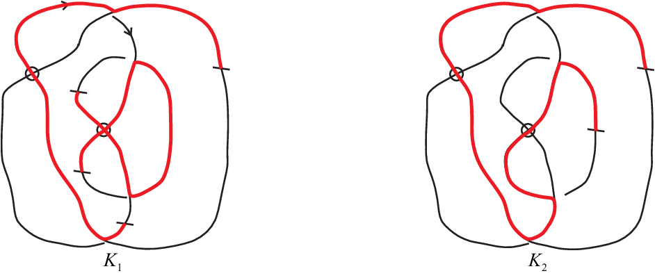
Let the underlying graph of a virtual link diagram with classical crossings be with 4-valent vertices. Since every edge of will have zero or one cut point, then we can get a set of dimension array modular 2, there are arrays. Denote the sets of all non-checkerboard framings and checkerboard framings by and , respectively. For any , we assume that the checkerboard colorings are and corresponding to and , respectively. Note that for any , there are two checkerboard colorings corresponding to it, we just arbitrarily choose one. It is obvious that for each classical crossing of , there are colorings and around its adjacent edges in and , respectively. Then colorings and are same or different. See one example as illustrated in Fig. 11. For checkerboard framing , if we use first move I for all classical crossings in where and are different as shown in Fig. 12, then we can obtain one new checkerboard framing and checkerboard coloring . Note that and only are different in some edges whose two endpoints are cut-points. Next we use move II in to reduce the cut-points such that the number of cut-point is 0 or 1 in each edge of , in the same time, the checkerboard coloring transforms to , that is, we obtain the checkerboard framing .

∎
Theorem 2.6.
Any two checkerboard framings of a diagram are related by a sequence of the cut point moves I and II (Fig. 7).
2.2. The checkerboard colorability of twisted links
The faces of a twisted link diagram are closed curves that run along the immersed curve and have the relationship with the crossings, virtual crossings, and bars as show in Fig. 13. At a crossing, a face turns so as to avoid crossing the link diagram. At a virtual crossing, a face goes through the virtual crossing. At a bar, a face crosses to the other side of the link diagram. A twisted link diagram is checkerboard colorable(or two-colorable in [3]) if its faces can be assigned one of two colors such that the arcs of the link diagram between two crossings always separate faces of one color from those of the other as show in Fig. 14.


Note that the three new twisted Reidemeister moves do not change the checkerboard colorability of a twisted link diagram. But the extended Reidemeister moves may change the checkerboard colorability of a checkerboard colorable twisted link diagram.
Let be a twisted link diagram, we denote the number of bars on by . Then, is the minimum number of bars contained in any twisted link diagram equivalent to . That is, the bar number of is
| (3) |
Theorem 2.7.
is a twisted link invariant.
Lemma 2.8.
Let be a checkerboard colorable twisted link diagram with classical crossings, then the number of bars on is even and after using move T1 and T2.
Proof.
has edges if we view each classical crossing and each bar as a 4-valent vertex and 2-valent vertex, respectively. If is a knot, the orientations of continuous two edges for a vertex alternate between “in” and “out”. For the first edge and the last edge to have different orientations, must have an even number of edges, that is, even number of bars is even.
If is a link diagram, it is possible for a component to share classical crossings with other components. This means that the component may have an odd number of edges. If the edges of the odd component have an alternate orientation, then the component has an odd number of bars. However, components of this type occur in pairs so that the total number of bars is even.
In the worst case scenario, every edge in its underlying diagram could have a bar after using move T1 and T2. If a diagram has crossings, then there would be bars. As a result, there is at most a bar on each edge and .
Since the underlying diagram of is a virtual link diagram, thus we can adapt the same formulation of Proposition 3.1 in [8]. We only formulate the same statement in different ways. ∎
Corollary 2.9.
For all twisted links , if , then is not a virtual link.
Corollary 2.10.
For all twisted links , let denote the minimum number of virtual crossings in any diagram of , then .
Note that if is a non-checkerboard colorable twisted link diagram, then is odd or even. We can place all bars near to virtual crossing such that the virtual crossings behave like classical crossings with regard to the checkerboard coloring.
Corollary 2.11.
Let be a checkerboard colorable twisted link. For any diagrams of , then is even.
Proof.
is even for checkerboard colorable diagram by Lemma 2.8. Based on the extended Reidemeister moves do not change the parity of the number of bars, we can obtain the conclusion. ∎
Note that the converse of this corollary is not true since there are non-checkerboard colorable virtual link diagram with zero bar.
We shall conclude this section by figuring out the connection and difference between Dye’s checkerboard framing and checkerboard coloring of twisted link diagram. It is obvious that we can construct a bijection between Dye’s checkerboard framing and checkerboard coloring of the corresponding twisted link diagram. For a virtual link diagram , let be a checkerboard framing of . Then we can obtain a checkerboard colorable twisted link diagram from by replacing each cut-point with a bar. Vice versa. Dye’s checkerboard framing is a combinatorial object, but checkerboard colorability of twisted link diagram is the property of the twisted link diagram. Thus, if we just focus on the checkerboard colorability of a diagram, then the role of cut-points in virtual link diagram and the role of bars in a twisted link diagram are the same. But bars in a twisted link diagram contain the topological construct of the diagram.
Let be a virtual link diagram. Let and be two checkerboard colorable twisted link diagrams obtained by adding some bars to . Then and maybe inequivalent as twisted links. See example of a pair of and in Fig 11. By computing their normalized arrow polynomials (see Section 3), , , then they are not equivalent by Theorem 3.4. Thus we can obtain a lot inequivalent of twisted links from by adding bars on diagrams.
Theorem 2.6 is true for checkerboard framings of a virtual link diagram, but the above example of a pair of and illustrates that it is not true if the cut-point is replaced with bars for twisted link diagrams and the cut point moves I and II are replaced with move T1, T2 and T3, since the move T3 may change the topological construct of the diagram.
3. Arrow polynomials of twisted links
In this section, we recall arrow polynomial of an oriented virtual link diagram defined by Dye and Kauffman [6] which is a criterion of detecting checkerboard colorability of virtual links in [5].
Let be an oriented virtual link diagram. We shall denote the arrow polynomial by the notation . The arrow polynomial of is based on the oriented state expansion as shown in Fig. 15. Note that each classical crossing has two types of smoothing, one oriented smoothing and other disoriented smoothing. Each disoriented smoothing gives rise to a cusp pair where each cusp is denoted by an angle with arrows either both entering the vertex or both leaving the vertex. Furthermore, the angle locally divides the plane into two parts: One part is the span of an acute angle (of size less than ); the other part is the span of an obtuse angle. The inside of the cusp denotes the span of the acute angle. It is obvious that the total number of cusps of a state circle after smoothing all classical crossing will be even according to the orientations on the edges of the state circle. The structure with cusps is reduced according to a set of rules that ensures invariance of the state summation under generalized Reidemeister moves. The basic conventions for this simplification are shown in Fig. 16. When the insides of the cusps are on opposite sides of the connecting segment (a “zig-zag”), then no cancellation is allowed. Each state circle is seen as a circle graph with extra nodes corresponding to the cusps. All graphs are taken up to virtual equivalence, as explained above. Fig. 16 illustrates the simplification of three circle graphs. In one case the graph reduces to a circle with no vertices. In the other case there is no further cancellation, but the graph is equivalent to one without a virtual crossing.
Note that the virtual crossings in a state have the potential to effect the total number of cusps. Use the reduction rule of Fig. 16 so that each state is a disjoint union of reduced circle graphs. Since such graphs are planar, each is equivalent to an embedded graph (no virtual crossings) via the detour move, and the reduced forms of such graphs have vertices that alternate in type around the circle so that are pointing inward (the angle of the cusp is obtuse in the inside of the circle) and are pointing outward (the angle of the cusp is acute in the inside of the circle). The circle with no vertices is evaluated as as is usual for these expansions, and the circle is removed from the graphical expansion. Let denote the circle graph with alternating vertex types as shown in Fig. 16 for and . Each circle graph contributes to the state sum and the graphs for remain in the graphical expansion. Each is an extra variable in the polynomial. Thus a product of the ’s corresponds to a state that is a disjoint union of copies of these circle graphs. Note that we continue to use the caveat that an isolated circle or circle graph (i.e. a state consisting in a single circle or single circle graph) is assigned a state circle value of unity in the state sum. This assures that is normalized so that the unknot receives the value one. Note that the arrow polynomial will reduce to the classical bracket polynomial when each of the new variables is set equal to unity.
Remark 3.1.
Formally, we have a state summation for the arrow polynomial of a twisted link diagram analogously to that of the virtual link diagram. For a state of , there maybe exist a circle graph with cusps and bars. For a twisted link diagram , we keep above rules and add some new rules for a state. If a reduced circle graph contains a cusp with two bars near it, we will reduce it as shown in Fig. 17. Generally, for a circle graph with cusps and several bars, if we consider a pair of bars, that is, one bar (resp. ) between cusps and (resp. and ), we assume that and without loss generality. Then we can insert a pair of bars between cusps and (), use the reduction rule of a cusp with two bars as shown in Fig. 17. That is, we will obtain a new circle graph with new cusps information but without bars. Then we will reduce to if the number of bars in is even or a trivial loop with a bar if the number of bars in is odd (as shown in Fig. 18) .


Definition 3.2.
([6]) The arrow polynomial of an oriented twisted link diagram is defined by
| (4) |
where runs over the oriented bracket states of the diagram, denotes the number of smoothings with coefficient in the state and denotes the number with coefficient , , is the number of circle graphs in the state, and is a product of extra variables and associated with the non-trivial circle graphs where is the number of trivial loops with a bar in the state . Note that each circle graph (trivial or not) contributes to the power of in the state summation, but only non-trivial circle graphs contribute to .
In [3], the writhe of twisted link diagram is a regular invariant of twisted link, that is, invariant under all extended Reidemeister moves except move RI. Let be an oriented twisted link diagram with writhe . The normalized version is defined by
| (5) |
For an oriented twisted link represented by an oriented link diagram , we denote by , and call it the normalized arrow polynomial of .
Note that there will not be bars in an oriented virtual link diagram, so does every state circle graph. Hence we will have the following conclusion as shown in [6].
Theorem 3.3.
([6], Theorem 1.6) Let be an oriented virtual link. Then is an invariant under the classical Reidemeister moves and virtual Reidemeister moves.
Theorem 3.4.
Let be an oriented twisted link. Then is an invariant under the extended Reidemeister moves.
Proof.
And it is obvious that we can get the following conclusion.
Theorem 3.5.
Let be an oriented twisted link diagram. The polynomial is an invariant under the extended Reidemeister moves except the Reidemeister moves RI.
By substituting for and for , turns into the polynomial (or ) defined by Kamada in [10]. By substituting for and for , turns into the polynomial the twisted Jones polynomial defined by Bourgoin in [3].
Example 3.1.
The twisted Jones polynomials of twisted links presented by the latter two diagrams in Fig. 1 are . On the other hand, our normalized arrow polynomial invariants of them are and , respectively. (They are also distinguished by the twisted link groups [3], which are the free product of their upper and lower groups.)
Note that if a reduced state has the form:
| (6) |
Then the -degree of the state is:
| (7) |
which is equal to the half of reduced number of cusps in the state associated with these variables. A surviving state is a summand of . The -degree of a surviving state is the -degree of any state associated with this summand. Notice that if the summand has no variables, then the -degree is zero.
Let denote the set of -degrees obtained from the set of surviving states of a diagram . The surviving states are represented by the summands of . That is, if is a summand of then 5 is an element of . If a twisted link has a total of 4 summands with subscripts summing to: 2, 2, 1, 0 then .
Lemma 3.6.
([6], Lemma 1.3) For an oriented virtual link diagram , is invariant under the virtual and classical Reidemeister moves.
Dye and Kauffman [6] showed that the phenomenon of cusped states and extra variables only occurs for virtual links.
Theorem 3.7.
([6], Theorem 1.5) If be a classical link diagram then .
Theorem 3.8.
For an oriented twisted link diagram , is invariant under the extended Reidemeister moves.
Proof.
We conclude it by Theorem 3.4. ∎
Next we shall determine the characteristics of arrow polynomials of checkerboard colorable twisted link diagrams. For this, we need to use the concept of twisted braid introduced by the author and the co-author in [19]. Let twisted braid be a -strands braid generated by , and as shown in Fig.20. For any , the generator elements satisfy the following relations:
| (8) |

Kauffman and Lambropoulou [17] gave a general method for converting virtual links to virtual braids. The braiding method given there is quite general and applies to all the categories in which braiding can be accomplished. It includes the braiding of classical, virtual, flat, welded, unrestricted, and singular knots and links. For a twisted link diagram, we just explain the braiding techniques for a classical crossing, a virtual crossing and a bar by three schemas as shown in Fig. 21, 22 and 23, we refer the reader to [17, 19].
We give a special example for the braiding process of a twisted link as shown in Fig. 24. We refer the reader to [17] and [19] for explanation.


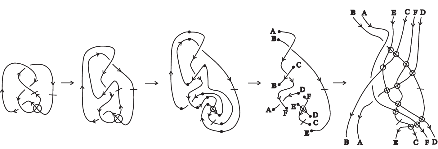
In Fig. 24 we illustrate an example of braiding the arcs of the diagram. In the first and second pictures we show a twisted knot and its preparation for braiding by crossing rotation, respectively. In the forth picture, we break each up-arc, and we name each pair of endpoints with the same letter. Note that the closure of the twisted braid in Fig. 24 is checkerboard colorable.
Theorem 3.9.
([17], Theorem 1) Every (oriented) virtual link can be represented by a virtual braid whose closure is isotopic to the original link.
Theorem 3.10.
([19]) Every (oriented) twisted link can be represented by a twisted braid whose closure is isotopic to the original link.
Proof.
Based on the proof of Theorem 1 in [17], we will adapt the similar technique for the case of twisted link. So we leave the proof to the reader. ∎
Remark 3.11.
According the braiding technique, described in Theorem 1 [17], which just changes the relatively position of classical and virtual crossings (resp. bars) by crossing rotation (resp. by moving), thus the original twisted link diagram and the closure of its twisted braid have the same checkerboard colorability.
We now determine the characteristics of arrow polynomials of checkerboard colorable twisted link diagrams. We have the following statement that figures out the characteristics of cusped states and extra variable for the arrow polynomials of checkerboard colorable twisted links.
Theorem 3.12.
Let be an oriented checkerboard colorable twisted link diagram. Then has
- (1)
does not contain ;
- (2)
only contains even integer;
- (3)
If contains a summand with (), then is even and .
Proof.
Since is checkerboard colorable, then each circle graph with bars or not is checkerboard colorable. Thus for each circle graph with bars will contain even bars. According to the above statement in Remark 3.1, this kind of circle graph will reduce to . Thus Theorem 3.12(1) holds.
Next we shall explain that the Theorem 3.12(2) and 3.12(3) for the case of twisted link diagram can be reduced to the case of virtual link diagram in [5] (Theorem 4.3(1) and (2)). The key is to reduce all bars and have the same characteristics.
By Theorem 3.10, we can arrange as twisted braid with all strands oriented downwards whose closure is isotopic to and checkerboard colorable. Note that and have the same set of classical crossings (see Fig. 24). Assume that is one checkerboard coloring of , in where we only draw one kind of color (yellow) to describe the coloring .
Let be an unreduced state of without applying reduction rule in Fig. 16. According to the coloring , we can obtain a checkerboard coloring of state , in where, the colorings of a small neighbourhood of one side of each arcs are the same with the coloring of except small segments of arcs around some classical crossings (see Fig. 25).

On the one hand, we assume that the cusp will be read as (or ) if the acute (or obtuse) angle of cusp and color (yellow) are on the same side in a circle graph. In all unreduced circle graphs of , there will be two s (or s) since the pair of acute angles of cusp and color (yellow) are on the same (or different) side. A circle graph will have a corresponding word if we read the cusp labeling (or ) of each classical crossing along a direction. Note that we do not read out the labeling of bars, that is, there is not in the word since the information of bars is transferred to the word. Note that the word is consistent with the virtual link diagram case in [5] (see the proof of Theorem 4.3).
On the other hand, if we first reduce all bars in each circle graph , then we will obtain a new circle graph such that the placement relation between acute angle of every cusp and color does not change as shown in Fig. 17. Thus the words of and should be the same.
Hence, the remain proof is consistent with the virtual link diagram case in [5] (see the proof of Theorem 4.3(1) and (2)). ∎
We can get the the same statement as Theorem 4 in [3].
Corollary 3.13.
If a twisted link has a checkerboard colorable diagram, then its twisted Jones polynomial is times its Jones polynomial.
Proof.
Let be a checkerboard colorable diagram of checkerboard colorable twisted link . Since does not contain , and we let in , then its twisted Jones polynomial is just times its Jones polynomial. ∎
Note that bar only deduce the cusps in circle graph.
Lemma 3.14.
Let be an oriented twisted link. Then is no less than the maximum degree of in .
Example 3.2.
For virtual knot with 2 classical crossings, there exists 4 inequivalent twisted knots (not virtual knot) as shown in Fig. 26. Their arrow polynomials are as follows. Thus the latter three twisted knots are non-checkerboard colorable by Theorem 3.12.
| (9) |
| (10) |
| (11) |
| (12) |

4. Acknowledgements
Deng is supported by Doctor’s Funds of Xiangtan University (No. 09KZKZ08069) and NSFC (No. 12001464). The project is also supported partially by Hu Xiang Gao Ceng Ci Ren Cai Ju Jiao Gong Cheng-Chuang Xin Ren Cai (No. 2019RS1057).
References
- [1] D. Bar-Natan, On Khovanov’s categorification of the Jones polynomial, Algebr. Geom. Topol., 2(2002)337-370.
- [2] D. Bar-Natan, S. Morrison, The Karoubi envelope and Lee’s degeneration of Khovanov homology, Algebr. Geom. Topol., 6(2006)1459-1469.
- [3] M. O. Bourgoin, Twisted link theory, Algebr. Geom. Topol., 8(3)(2008)1249-1279.
- [4] J. S. Carter, S. Kamada, M. Saito, Stable equivalence of knots on surfaces and virtual knot cobordisms, J. Knot Theory Ramifications, 11(2002)311-322.
- [5] Q. Deng, X. Jin, L. H. Kauffman, On arrow polynomials of checkerboard colorable virtual links, arXiv:2002.07361.
- [6] H. A. Dye, L. H. Kauffman, Virtual crossing number and the arrow polynomial, J. Knot Theory Ramifications, 18(10)(2009)1335-1357.
- [7] H. A. Dye, A. Kaestner, L. H. Kauffman, Khovanov homology, Lee homology and a Rasmussen invariant for virtual knots, J. Knot Theory Ramifications, 26(3)(2017)ArticleID: 1741001, 57pp.
- [8] H. A. Dye, Cut points: An invariant of virtual links, J. Knot Theory Ramifications, 26(9)(2017)ArticleID: 1743006, 10pp.
- [9] T. Imabeppu, On Sawollek polynomials of checkerboard colorable virtual links, J. Knot Theory Ramifications, 25(2)(2016)ArticleID: 1650010, 19pp.
- [10] N. Kamada, The polynomial invariants of twisted links, Topology and its Applications, 157(2010)220-227.
- [11] N. Kamada, S. Kamada, Virtual links which are equivalent as twisted links, Proc. Amer. Math. Soc., 148(5)(2020)2273-2285.
- [12] N. Kamada, S. Kamada, Abstract link diagrams and virtual knots, J. Knot Theory Ramifications, 9(1)(2000)93-106.
- [13] N. Kamada, On the Jones polynomials of checkerboard colorable virtual links, Osaka J. Math., 39(2)(2002)325-333.
- [14] N. Kamada, Span of the Jones polynomial of an alternating virtual link, Algebr. Geom. Topol., 4(2004)1083-1101.
- [15] N. Kamada, S. Nakabo, S. Satoh, A virtualized skein relation for Jones polynomials, Illinois J. Math., 46(2)(2002)467-475.
- [16] L. H. Kauffman, Virtual knot theory, European J. Comb., 20(1999)663-690.
- [17] L. H. Kauffman, S. Lambropoulou, Virtual braids, Fund. Math., 184(2004)159-186.
- [18] Y. Miyazawa, Magnetic graphs and invariant for virtual links, J. Knot Theory Ramifications, 15(2006)1319-1334.
- [19] S. Xue, Q. Deng, Twisted braid, (in preparation).