A stabilized computational nonlocal poromechanics model for dynamic analysis of saturated porous media
Abstract
In this article we formulate a stable computational nonlocal poromechanics model for dynamic analysis of saturated porous media. As a novelty, the stabilization formulation eliminates zero-energy modes associated with the original multiphase correspondence constitutive models in the coupled nonlocal poromechanics model. The two-phase stabilization scheme is formulated based on an energy method that incorporates inhomogeneous solid deformation and fluid flow. In this method, the nonlocal formulations of skeleton strain energy and fluid flow dissipation energy equate to their local formulations. The stable coupled nonlocal poromechanics model is solved for dynamic analysis by an implicit time integration scheme. As a new contribution, we validate the coupled stabilization formulation by comparing numerical results with analytical and finite element solutions for one-dimensional and two-dimensional dynamic problems in saturated porous media. Numerical examples of dynamic strain localization in saturated porous media are presented to demonstrate the efficacy of the stable coupled poromechanics framework for localized failure under dynamic loads.
Keywords:
stabilization , nonlocal , coupled , poromechanics , dynamics , saturated porous media1 Introduction
Dynamic behavior of deforming porous media is significant problem in engineering and science [1, 2]. A fully coupled dynamic analysis of porous media is essential in earthquake engineering (soil liquefaction), geo-hazard engineering (dynamics landslide triggering), and offshore wind industry (wind turbine foundations) [3, 4]. The integrity of civil infrastructure (e.g., dams and levee systems) can be seriously compromised by the poor performance of soils under dynamic loading conditions. Thus, numerous researchers have studied the dynamics and wave propagation characteristics of saturated porous media, e.g., [5, 6, 7, 8, 9] among others. One typical failure of porous media under dynamic loads is dynamic strain localization (e.g., [10, 2]). A topic has been insufficiently studied compared to the extensive research on strain localization of porous media under static or quasi-static loading conditions (see [11] and [12] for a recent review). Over the past decades, viscoplasticity has been adopted to study dynamic strain localization of solid or porous media (see [13, 10, 14, 15, 16, 17], among others), as well as a means of regularizing the rate-independent problem so that the governing equation of dynamic problems remains hyperbolic. Heider et al [15] developed a a coupled dynamic elasto-viscoplastic model for sands and found that inertial loads had a significant impact on dynamic strain localization. Shahbodagh et al [16] proposed an elasto-viscoplastic model for dynamic analysis of strain localization in fully saturated clay. The above methods are based on the classic local poromechanics. It has been generally recognized that nonlocal models are robust to investigate mulitphysics failure mechanisms including the dynamic strain localization phenomenon in porous media (e.g., [18, 19, 20, 21] and many others). In this article, we propose a stabilized coupled nonlocal poromechanics model to study dynamic strain localization in saturated porous media.
In [22], a computational periporomechanmics model was formulated to model localized failure in unsaturated porous media under static condition. The coupled nonlocal model in [22] was formulated based on the peridynamic state concept [23], the effective force state concept and multiphase correspondence principle [24]. We refer to the literature for other nonlocal models for porous media (see [25, 26, 27, 28, 29, 30, 31, 32], among others), which are formulated using peridynamics theory (i.e., the bond-based or ordinary state-based peridynamics) [33, 23, 26] and poroelasticity (see [34]). It was demonstrated that the coupled nonlocal model in [24] is robust for modeling localized failure in unsaturated soils under static/quasi-static loading conditions. However, it is recognized that the peridynamics model formulated based on the correspondence principle for the single-phase solid has stability issues under extreme large deformation and dynamic loading conditions (e.g., [35, 36, 37, 38, 39, 40, 41, 42, 43, 44, 45], among others). Silling [38] showed that the numerical oscillation in peridynamics material models formulated via the single-phase correspondence principle [23] is associated with material instability instead of merely an artifact of the meshless discretization [46]. This study suggests that the primary causes of instability and numerical oscillations are (1) the weak dependence of the force density in a bond on its own deformation and (2) the loss of the non-uniform part of deformation due to the integration over the horizon of a material point. Note that the above studies and remedies for the instability were focused on modeling the large deformation or extreme damage of single-phase solid materials through the original correspondence principle [23]. Here for the first time we prove that the recently formulated multiphase correspondence for modeling unsaturated porous media inherit the aforementioned instability under large deformation and dynamic loading conditions. To circumvent the issue, we have formulated the coupled stabilization terms for solid deformation and fluid flow respectively in Section 2.
In this article, we formulate and implement a stabilized coupled nonlocal poromechanics model for dynamic strain localization in saturated porous media. As a novelty, the stabilization terms eliminates zero-energy modes associated with the multiphase correspondence constitutive models in the coupled nonlocal framework for modeling saturated porous media under dynamic loads. The stabilization terms are formulated based on the energy method in which the nonlocal formulations of skeleton strain energy and fluid flow dissipation energy equate to their local formulations in line with the classical poromechanics for saturated porous media. Specifically, the method incorporates non-homogeneous solid deformation and fluid flow around a material point. The stabilized coupled nonlocal poromechanics model is numerically solved using a hybrid Lagrangian-Eulerian meshless method with an implicit time integration scheme. Parallel computing is also adopted for computational efficiency. The coupled stabilized formulation is validated by comparing numerical results with analytical and finite element solutions for one-dimensional and two-dimensional dynamic problems in saturated porous media. Numerical examples of dynamic strain localization in saturated porous media are presented to demonstrate the efficacy of the stable coupled poromechanics framework for localized failure under dynamic loads. We note that the stabilized coupled nonlocal model for saturated porous media can be readily extended to model dynamic problems in unsaturated porous media.
The contribution of this article includes (1) a proof of the zero-energy modes associated with the original multiphase correspondence constitutive principle for modeling porous media through multiphase peridynamic states, (2) a remedy based on the energy method to remove the multiphase zero-energy modes for dynamic analysis, and (3) an implicit numerical implementation of the proposed stabilized dynamic non-local poromechanics model and its validation. For sign convention, the assumption in continuum mechanics is followed, i.e., for solid skeleton, tensile force/stress is positive and compression is negative, and for fluid compression is positive and tension is negative.
2 Stabilized nonlocal formulation for coupled dynamics problems
For conciseness of notations, it is assumed that the peridynamic state variable without a prime means that the variable is evaluated at on the associated bond and the peridynamic state variable with a prime means that the variable is evaluated at on the associated bond , e.g., and .
2.1 Dynamic saturated periporomechanics model
Periporomechanics is a fully coupled, nonlocal theory of porous media. It is a reformulation of classical poromechanics through peridynamics for modeling continuous or discontinous deformation and physical processes in porous media [24, 22]. In periporomechanics, it is assumed that a porous media body is composed of material points which have two kinds of degree of freedom, i.e., displacement and fluid pressure. A material point has poromechanical and physical interactions with any material point within its neighborhood, . Here is a spherical domain around with radius , which is called the horizon for the porous medium. Let be the density of the two phase mixture that is determined by
| (1) |
where and are the intrinsic density of the solid and the fluid, respectively, and is the porosity (i.e., the volume of pore space divided by the total volume). Figure 1 shows the schematics of the kinematics of two material points.

The relative position of material points and in the reference configuration is denoted by
| (2) |
Let the displacements of and be and respectively. The relative displacement between and in the deformed configuration is
| (3) |
The position vectors and of and in the deformed configuration are
| (4) |
The deformation state of on is defined as
| (5) |
The fluid potential state at imposed on is defined as
| (6) |
where and are pore fluid pressures at and , respectively.
| (7) |
where and the effective state and the fluid phase force state at material point , is the gravity acceleration, and is the acceleration vector. Assuming an incompressible solid phase, the fluid mass balance equation incorporating the volume change of the solid skeleton reads
| (8) |
where is fluid pressure, is the bulk modulus of fluid, and are the rate of volume change scalar states of the solid at and , respectively, and are fluid mass flow scalar states relative to the solid skeleton at and , respectively.
Through the multiphase correspondence principle [24], the effective force state and the fluid mass flow state can be determined by the peridynamic constitutive models via the deformation state of the solid skeleton and the fluid potential state, respectively. The momentum balance equation for saturated porous media in periporomechanics under dynamic loading reads
| (9) |
where is a scalar influence function, is the nonlocal deformation gradient, is the determinant of , is the effective stress tensor that can be determined by classical constitutive models given , is the second-order identity tensor, and is the shape tensor. The nonlocal deformation gradient is defined as
| (10) |
It is assumed that the accelerations of the fluid and the solid are identical [1]. Through the multiphase correspondence principle [24], the fluid mass balance equation accounting for the volume change of the solid skeleton reads
| (11) |
where is the bulk modulus of fluid, and are the fluid flux vectors at and respectively and is the hydraulic conductivity. The fluid flux can be determined by Darcy’s law as
| (12) |
where is hydraulic conductivity, and is the approximate nonlocal fluid pressure gradient,
| (13) |
2.2 Two-phase stabilization formulation
As stated in the multiphase correspondence principle [24], the nonlocal deformation gradient and fluid pressure gradient are approximate for the non-uniform deformation and fluid flow while they are exact for the uniform deformation and fluid flow respectively. There can be increments that may have no effect on the approximate deformation gradient, leading to zero-energy modes of deformation [38]. Similarly, for fluid flow there can be increments that may have no effect on the approximate fluid pressure gradient, leading to zero-energy modes of fluid flow. It can be demonstrated as follows. The nonuniform part of the solid deformation state and fluid potential state can be defined as
| (14) | ||||
| (15) |
Substituting equations (14) and (15) into (10) and (13) generates
| (16) |
| (17) |
For the solid skeleton, the strain energy density is assumed as
| (18) |
where is the stored energy from the standard correspondence material model, and
| (19) |
where is a prescribed positive-valued scalar state. Given a small increment , it follows from (14) and (19) that
| (20) |
where . It follows from (20) that the stablized term for the effective force state accounting for the non-uniformed deformation state can be written as
| (21) |
Given it can be proved that is always positive for a positive value of . It follows from (21) along with the original multiphase correspondence principle [24] that the stabilized effective stress state can be written as
| (22) |
To simplify (22), it is assumed that
| (23) |
where is a positive constant on the order of 1 and is a micromodulus which will be provided in the next section. With (23) and (16), it can be proved that the third term of (22) becomes zero. Thus, equation (22) can be expressed as
| (24) |
Similarly, for the fluid phase the energy dissipation accounting for the non-uniform fluid potential state can be written as
| (25) |
where is the energy dissipation related to the uniform fluid potential through the corresponding Darcy’s law (i.e., (12)) and is the dissipation energy through the non-uniform fluid potential. It is assumed that takes the general form
| (26) |
where is a positive-valued scalar state. Given a small increment , it follows from (17) and (26) that
| (27) |
where . It follows from (27) that the stabilized term for the fluid flow state accounting for the non-uniform fluid potential state can be written as
| (28) |
Given it can be proved that is always positive for a positive value of . From (28) and the original multiphase correspondence principle [24] the stabilized fluid flow state can be written as
| (29) |
To simplify (29), it is assumed that
| (30) |
where is a positive constant on the order of 1 as defined earlier and is a micro-conductivity which will be derived in the next section. With (30) and (17), it can be shown that the third term of (29) becomes zero. Thus, equation (29) can be expressed as
| (31) |
2.3 Determination of stabilization parameters
In this part the parameters in the stabilized terms will be derived based on the energy equivalence between peridynamics and classical theory for the solid skeleton and fluid phase. For the solid phase, it is postulated that the stored elastic energy in the solid skeleton from peridynamics equals to the elastic energy from the classical poromechanic theory at the same material point .
For simplicity, a microelastic peridynamic model [46] is adopted to determine the elastic energy in the solid skeleton at material point . In the microelastic material model, the effective pairwise force function that material point imposes on material point is determined from a micropotential as
| (34) |
where and . The micro-potential function is a measure of the elastic strain energy stored in a single bond of the solid skeleton due to its deformation. The total strain energy density at point is expressed as
| (35) |
where the factor of means that each endpoint of a bond between two solid material points owns only half the energy in this bond. Let be the magnitude of as
| (36) |
We further assume a homogeneous solid skeleton under isotropic extension. It follows
| (37) |
where is a constant for all . Thus can be written as
| (38) |
where is the constant defined previously. It follows from (36) and (38) that
| (39) |
Substituting (39) into (35) gives
| (40) |
The elastic strain energy of the solid skeleton at material point from the classical elastic theory under isotropic deformation is
| (41) |
where is the classical elastic bulk modulus and is the elastic volumetric strain. Combining (40) and (41) leads to an expression for under three-dimensional condition as
| (42) |
For the fluid phase, the pairwise fluid flow density at material point in the bond-based peridynamics can be determined from a fluid dissipation micropotential through
| (43) |
where is the fluid pressure difference between material points and . The dissipation micropotential represents the dissipation potential along a bond between two material points and is a function of the fluid potential scalar state of that bond. Then the total dissipation potential at point is a summation over all the micropotentials in the family of this point.
| (44) |
where similar to the solid phase the factor of means that each endpoint of a bond between two solid material points owns only half the energy in this bond. The pairwise fluid flow density at is assumed as
| (45) |
where is the peridynamic hydraulic micro-conductivity. It follows from () and (43) that fluid flow dissipation micro-potential can be written as
| (46) |
The peridynamic hydraulic micro-conductivity can be related to the classical hydraulic conductivity by equating the peridynamic fluid dissipation potential to the classical fluid dissipation potential at point . For simplicity, we assume a linear pressure field in a body, for a three-dimensional case. Thus, the fluid pressures at material points and are written as
| (47) |
It follows that
| (48) |
Substituting (47) into (46) and conducting integration in a sphere with radius centered at lead to
| (49) |
Assuming a homogeneous body and isotropic fluid flow, the classical fluid dissipation energy through Darcy’s law at material point is expressed as
| (50) |
where is the hydraulic conductivity of saturated porous media. It follows from (50) and (47) that the classical fluid dissipation energy at material point is
| (51) |
Combining (49) and (51) gives the hydraulic micro-conductivity under three-dimensional condition as
| (52) |
3 Numerical implementation
3.1 Spatial discretization
The equations (32) and (33) are spatially discretized by a hybrid Lagrangian-Eulerian meshfree scheme, as shown in Figure 2. In this method, a porous continuum material is discretized into a finite number of mixed material points (i.e., mixed solid skeleton and pore water material points). Each material point has two types of degree of freedom, the displacement and the pore water pressure. The uniform grid is used to spatially discretize the problem domain in which all material points have an identical size.

It is assumed that inertia loading has no impact on the fluid flow [1] and water is incompressible. Let be the number of material points in the horizon of a material point . The spatially discretized equations at material point can be written as
| (53) | ||||
| (54) |
where
| (55) | ||||
| (56) | ||||
| (57) | ||||
| (58) | ||||
| (59) |
We define the linear assembly operator [47]. Let be the number of the total material points. The global discretization form of the coupled equations can be written as
| (60) | ||||
| (61) |
3.2 Time integration and linearization
We formulate a fully implicit scheme to integrate the coupled system of equations in time[47]. At , the residual vector of the the coupled system is defined as
| (62) | ||||
| (63) |
The Newmark method [48, 1] is adopted. In the temporal domain a second-order scheme is used to integrate the momentum balance equation and a first-order scheme is applied to integrate the mass balance equation. At time step , , , , , and are known. Let and , the acceleration, velocity, displacement and water pressure vectors at can be written as follows,
| (64) | ||||
| (65) | ||||
| (66) | ||||
| (67) |
where are numerical integration parameters. For unconditional stability,
| (68) |
Substituting (64), (65), (66), and (67) into (62) and (63), and , can be solved by Newton’s method as follows. Let be the iteration number.
| (69) |
where
| (70) |
By solving (69), we have
| (71) |
Finally, we have
| (72) |
3.3 Tangent operator
Given the relationships in equation (64) - (67), by chain rule the individual components of can be written as follows.
| (73) | ||||
| (74) | ||||
| (75) | ||||
| (76) |
where is the global solid tangent operator, and are the global coupling matrices, is the global fluid tangent operator, is the second-order identity tensor with the dimension of the number of total material points in the problem domain, and for brevity we define
| (77) | ||||
| (78) |
Inspired by the standard procedure in the finite element method [47], the stiffness matrix here will be constructed from the corresponding local stiffness matrices at material points. In this article, the stiffness matrix at a material point will be first computed and then the assembly operator will be utilized to construct the global stiffness matrix. In what follows, the derivation is focused on the stiffness matrices at one material point incorporating all the material points in its horizon.
We linearize the momentum balance equation at material point by following the chain rule. The incremental forms of and at material point can be written as
| (79) | ||||
| (80) |
where .
It follows from (79) and (80) that we have
| (81) | ||||
| (82) | ||||
| (83) | ||||
| (84) |
where and can be determined from a peridynamic material model (e.g., ordinary or non-ordinary). For brevity of notations, let us define
| (85) | ||||
| (86) |
For the dynamic loading term, , we define,
| (87) | ||||
| (88) |
where
| (89) | |||
| (90) |
Therefore, from (81) - (88), the solid tangent matrix at material point can be constructed as
| (91) |
where is a matrix with dimensions .
Similarly, it follows from (79) that we have
| (92) | ||||
| (93) |
Thus, the coupling matrix at material point can be constructed as
| (94) |
where is a matrix with dimensions .
Next, we derive the tangent matrices associated with the mass balance equation at material point . The linearization of and at point can be written as
| (95) | |||
| (96) |
where . From (95) and (96) we obtain
| (97) | ||||
| (98) | ||||
| (99) | ||||
| (100) |
For brevity of notations, let us define
| (101) | |||
| (102) |
It follows from (101) and (102) that the flow tangent matrix at point can be written as
| (103) |
where is a row vector with the dimension . For the rate of the solid volume change, it can be readily derived by chain rule that
| (104) | ||||
| (105) |
Thus, the coupling tangent matrix at material point can be written as
| (106) |
where is a vector with the dimensions of .
Finally, the global tangent matrix can be constructed from (), (103), (94), and (106) for all material points.
| (107) | ||||
| (108) | ||||
| (109) | ||||
| (110) |
where is the assembly operator that constructs the global stiffness matrix from the tangent matrices at individual point. In the computer code, each material point and material points in its horizon are assigned a unique global identification (ID) number that are used by to construct the global tangent matrix. Indeed the assembly procedure adopted here is exactly the same as the global stiffness assembly operator in the finite element method [47]. Algorithm 1 summarize the general procedure for the computation of local tangent matrices at the material point level and the assembly of the global tangent matrix. Parallel computing through Open MPI [49] is exploited to increase the computational efficiency of the stabilized coupled periporomechanics model.
3.4 Linearization of correspondence material models
We present the material-point level linearization of correspondence solid and fluid models implemented in this study. Now, the differentiation of the total force density at a material point with respect to a deformation state reads,
| (111) |
where can be determined through the return mapping algorithm following the lines in computational plasticity (e.g., [50, 51, 52], and others)
| (112) | ||||
| (113) |
The linearization of the stabilization force with respect to a deformation state reads,
| (114) |
where and is nonzero only if . Next, the momentum balance linearized with respect to the fluid pressure reads,
| (115) | ||||
| (116) |
Similarly, for the mass balance, the derivative of fluid flow density with respect to a pressure potential state reads,
| (117) |
where
| (118) | ||||
| (119) |
The linearization of the stabilization flow density with respect to a deformation state reads
| (120) |
where and are nonzero only if .
4 Numerical examples
For the numerical examples in this section we adopt the time integration parameters in the literature that satisfy the criteria for unconditional stability and high frequency numerical dissipation [1, popescu1993centrifuge]. For all three examples in what follows we have and . All boundary conditions are imposed through a fictitious boundary layer (see [33, 23, 26]).
4.1 Correspondence material models
For the material models, we implement two classical material models for the solid skeleton and the classical Darcy’s law for fluid flow through the extended correspondence principle with stabilization. Following the lines in continuum mechanics [50], the total strain can be determined from the nonlocal deformation gradient at a material point. In examples 1 and 2, the solid skeleton is modeled by an isotropic elastic constitutive relationship, which reads
| (121) |
where , is the isotropic elastic tensor, and is the elastic strain tensor. The isotropic elastic tensor is written as
| (122) |
where is the shear modulus and is the rank-four identity tensor.
In example 3, the critical-state based elastoplastic model for saturated soils [53, 54] is adopted and numerically implemented through the celebrated return-mapping algorithm in computational plasticity [50, 55]. In this material model, the total strain tensor is additively decomposed into the elastic strain tensor and the plastic strain tensor as
| (123) |
Given the elastic strain tensor, the effective stress can be computed by equation (121). The yield function is written as
| (124) |
where is the effective mean stress, is the equivalent shear stress, is the slope of the critical state line, and is the preconsolidation pressure. As a hardening law, evolves with plastic volumetric strain.
| (125) |
where and are the swelling index and the compression index, respectively. The plastic strain is determined below by assuming the associative flow rule.
| (126) |
where is the non-negative plastic multiplier. It is noted that advanced constitutive models for geomaterials can be applied in the formulated peridynamics poromechanics in this article by the recently proposed multiphase correspondence principle (see [24]).
4.2 One-dimensional dynamic consolidation problem
This example concerns the one-dimensional dynamic consolidation of a saturated soil specimen under instantaneous and sinusoidal loading conditions, respectively. Numerical results from the coupled peridynamics (PD) model are compared with the analytical and finite element (FE) solutions in the literature [56, 57].
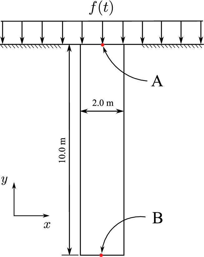
Figure 3 depicts the geometry of the soil column. The load is imposed on the top boundary. The soil column is restricted to deform vertically while the bottom is fixed. For the fluid phase, the top boundary is drainage and all other boundaries are impervious. The initial effective stress and water pressure are not taken into account as assumed in [56, 57]. The problem domain is discretized into 25,000 mixed material points. The center-to-center distance of two neighboring material points is = 0.04 m.
4.2.1 Instantaneous load

Figure 4 plots the instantaneous load imposed on the top of the specimen. The simulation time s and the time increment = 1 s [56]. The solid skeleton is modeled by a correspondence elastic model. The fluid flow is modeled by the correspondence Darcy’s law. The material parameters adopted from [56] are: bulk modulus kPa, shear modulus kPa, kg/m3, initial porosity , = kPa, kg/m3, m/s. The horizon . The simulation time s and the time increment s.
Figure 5 plots the coupled PD solutions with different values of parameter and analytical solution of the vertical displacement at A shown in Figure 4. Figure 6 compares the PD solutions with different values of parameter and analytical solution of the water pressure at B shown in Figure 4.


It is shown from Figure 5 that the value of can have a significant effect on the predicted amplitude of the oscillations of the vertical displacement at point A. For = 0, the PD results of vertical displacement are in good agreement with the analytical solution early in the simulation, with the triangular waveform of the analytical solution being largely preserved. These oscillations in amplitude diminish over time due to fluid viscous dissipation, and will eventually go to zero. However, the oscillations in the PD solution appear to dissipate more rapidly than the analytical solution. With , the PD solution approaches the analytical one, with = 1.0 giving the best results. It is also apparent that increasing the value of , appears to have a negligible influence on the PD solutions, with practically no difference in the results obtained for = 1 and = 2.
The water pressure response at B as shown in Figure 6 takes the form of periodic square waves of a constant amplitude. For = 0, the PD solution has noticeable high-frequency oscillations at the peak and valley of the square waves. It is apparent that almost eliminates high-frequency oscillations in the plot of water pressure. Increasing the value of to 1 or 2 does not improve the accuracy of the PD solution with respect to the analytical one. Indeed, a value of = 2 may decrease the period of the PD wave shown in the analytical wave profile.
4.2.2 Sinusoidal load

The sinusoidal loading profile as shown in Figure 7 is expressed as
| (127) |
where the angular frequency = 20 radians/s. The total simulation time = 0.5 s and the time increment = 1 s. The solid skeleton is modeled by a correspondence elastic model and the fluid flow is modeled by the correspondence Darcy’s law. The input material parameters adopted from [58] are: kPa, kPa, kg/m3, , kPa, kg/m3, and m/s. The horizon . The initial and boundary conditions are identical to the instantaneous loading scenario.
Figure 8 plots the vertical displacement at the point A in Figure 3 over time from the PD solution and the analytical and FE solutions. Figure 9 plots the water pressure at the point B in Figure 3 over time from the PD solution and the FE solution.


The results in Figure 8 show that the PD solution generally matches the analytical and FE solutions of the vertical displacement at the point A. It is found that the value of slightly affects the PD solution in this case. With = 0, the PD solution of the displacement is close to the analytical solution at the peaks of the displacement profile. However, the PD solution diverges from the analtyical solution at the valleys of the displacement profile. With the PD solution generated a uniform decrease in the amplitude of the oscillations of the displacement profile. Figure 9 shows that the PD solution with of the water pressure with = 1.0 is close to the FE solution. There is no noticeable change in the PD solution with = 2.0.
The influence of the stabilization parameter on the solid skeleton and pore fluid discussed in this example is consistent with the results obtained from the quasi-static analysis of the solid material [45]. It was found that for simple elastic problems values as low as 0.01 could provide maximum reduction in relative errors with the analytical solution. Increasing the value of G may gradually lead to an increase of the relative error over the non-stabilized case. Larger values of G may be required when modeling fracture propagation or finite deformation. In the dynamic analysis of solids in [38], it was suggested the value of should be in the order of 1 for high strain rates and large deformation.
4.3 Wave propagation in saturated soil
This example deals with a two-dimensional saturated soil specimen under dynamic loading through a strip footing. The numerical results from PD are compared with the FE solutions in the literature [58].
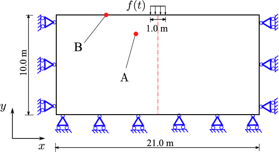
Figure 10 depicts the problem geometry and the boundary conditions. For the fluid phase, the fluid pressure at the top boundary is set to zero. The remaining boundaries are impermeable. The solid skeleton is modeled by a correspondence elastic model and the fluid flow is modeled by the correspondence Darcy’s law. The problem domain is discretized into 100,000 uniform mixed material points with = 0.05 m. m. The input material parameters adopted from [59, 60, 58] are: kPa, kPa, kg/m3, , = kPa, kg/m3, m/s.

As in [59, 60, 58], the problem domain is prescribed with null initial effective stress and water pressure. The dynamic load is imposed on a strip footing on the top surface as shown in Figure 11.
| (128) |
where is equal to 1 if s, and is zero if s. The simulation time = 0.2 s and s.


Figure 12 compares the PD solutions with different values of and FE solutions [58] of the water pressure at the point A. With = 0, the PD solution of the water pressure at point A slightly lags behind the FE solution and there are some oscillation at s . The plot of water pressure with = 0.1 is smooth and closely matches the FE solution. The PD solutions with larger values of seem to generate mild changes in the plot of water pressure. Figure 13 compares the PD solutions with the FE solutions of the vertical displacement (heave) versus the horizontal displacement at point B. The results show the expected elliptical motion at the point A under the dynamic load on the top boundary.
Figure 14 plots the contour of the magnitude of displacement in the problem domain from the PD solution and the FEM solution at 0.05 s, 0.1 s, 0.15 s and 0.2 s. In the PD solution, it is assumed = 0.05.

The results in Figure 14 demonstrate that the PD solution is consistent with the FE solution in [58]. Both the PD and FE solutions show two-dimensional wave propagation through the bulk of the poroelastic medium. with the surface showing elliptic motion by the dynamic load. The amplitude of this wave decreases as it travels farther away from the strip footing. Given the spike load profile, the deformation energy slowly dissipates as the wave moves through the problem domain that reduces the amplitude.
4.4 Dynamic strain localization in a two-dimensional soil specimen
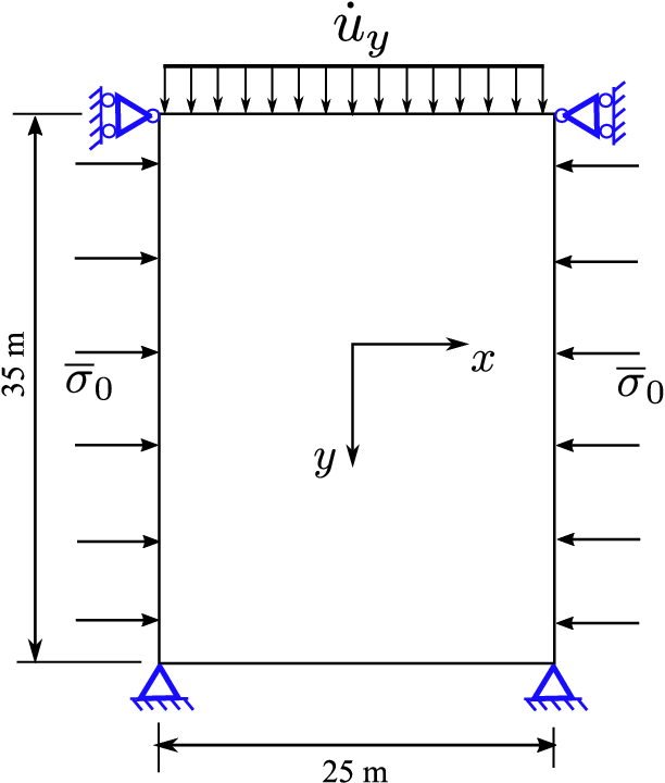
In this example we simulate dynamic strain localization in a two-dimensional saturated soil sample subjected to a vertical compression. The problem geometry adopted and boundary conditions applied are shown in Figure 15.
The problem domain is discretized into 20,000 mixed material points with = 0.3 m and volume m3. The material parameters used are : kg/m3, kPa, kPa, , initial pre-consolidation pressure kPa, = 0.03, = 0.10, = 1.0, kg/m3, kPa, m/s. The horizon is set to 2.05. The stabilization parameter = 0.025 is chosen to avoid excessive influence on the post-localization behavior [38].
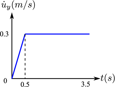
For the initial state the problem domain has an isotropic mean effective stress -100 kPa and zero water pressure. The skeleton boundary conditions are depicted in Figure 15, where is a lateral confining pressure of 100 kPa. For the fluid phase, all boundaries are impermeable. The velocity load as shown in Figure 16 is imposed on the top boundary. The simulation time at = 3.5 s and the time increment = 5 s.
Figures 17, 18 and 19 draw the contours of the equivalent shear strain, plastic volume strain and water pressure at = 1.0 s, 2.0 s, and 3.0 s, respectively. The corresponding displacements on the top boundary are = 0.225 m, 0.52 m, 0.83 m, respectively. Here the equivalent shear strain is the second invariant of the strain tensor , i.e., =.


The results show that the deformation and pressure have localized into symmetric banded zones. At = 1.0 s, plastic deformation has initiated and propagated diagonally through the specimen (Figures 17 and 18 (a)). We observe a similar behavior in the fluid pressure field (Figure 19(a), where localization manifests as regions of decreased water pressure. In Figure 17 (b) and (c) shows that plastic deformation progressively resolve into sharply defined zones of intense shear deformation. However, in the contours of plastic volume strain (see Figure 18 (b) and (c)) and water pressure (see Figure 19(b) and (c)) the banded zones appear to be more diffusive. The plastic volume change in the banded deformation is positive denoting dilatation. As such, the increase in skeleton volume leads to decrease in the water pressure inside the banded zone. The dilatation under dynamic loading can be expected for a moderately over-consolidated soil specimen. Due to the relatively large permeability chosen, the pore water can readily move into the zones of plastic dilatation, leading to more diffuse zones of water pressure.
4.4.1 Sensitivity to spatial discretization
In what follows, we present a discretization sensitivity analysis to demonstrate that the dynamic strain localization problem remains well-posed through the proposed nonlocal formulation. We rerun the numerical simulation with a fine spatial discretization. The fine spatial discretization consists of 43000 mixed material points with = 0.2 m. For comparison, all material parameters and conditions remain the same. Figures 20 and 21 compare the equivalent shear strain and water pressure respectively from the simulations with the coarse and fine discretizations at = 0.83 m. The results in Figures 20 show that the contours of the equivalent shear strain from both simulations are almost identical. The same conclusion can be drawn from Figure 21 regarding the water pressure. It can be concluded that both he location and orientation of the shear band are independent of the spatial discretization.


In Figures 22 and 23 we plot the variation of equivalent plastic shear strain and water pressure along a horizontal line at 10 m above the specimen center at = 3.0 s. The values of equivalent shear strain and water pressure are identical for both discretizations. It is known that in the dynamic strain localization analysis by FEM the mesh dependence of plastic strain and water pressure in the banded zone can be resolved by using a viscoplasticity model [10, 16]. However, the width of the banded zone still showed some sensitivity to the spatial discretization scheme (element size).


4.4.2 Influence of dynamic loading
We investigate the influence of dynamic loading rates on the coupled response during dynamic strain localization. The base simulation with m/s is repeated with m/s and = 1.5 m/s respectively. All other material parameters and conditions remain the same. The results are compared at an identical displacement of the top boundary. Figures 24, 25 and 26 show the contours of the equivalent shear strain, plastic volume strain and water pressure respectively at = 0.5 m on the top boundary for three different dynamic loading rates.


The results these Figures show the loading rate impact the formation of banded deformation and pressure zones. For = 0.3 m/s, it is apparent that the contour of plastic deformation as shown in Figures 24 and 25 (a) and the contour of water pressure as shown in Figure 26(a) have localized into a single pair of two conjugate banded zones. For the simulations with two larger loading rates, = 0.9 m/s and 1.5 m/s, two distinct pairs of localized deformation bands are formed in the solid skeleton as shown in Figures 24 and 25 (b). Consistent with the skeleton deformation, the contour of water pressure also shows two pairs of banded zones as shown in Figure 26(b). It can be concluded from the results in Figures 24, 25 and 26 that the dynamic loading rate impacts the number, location and orientation of shear bands in unsaturated porous media.
Figure 27 plots the reaction force over the applied vertical displacement for the three different loading rates. The results show that the specimen under a higher dynamic loading rate shows a higher peak value in the loading capacity. The oscillations in the reaction force curves with larger loading rates may be correlated to locally undrained condition under these loading condition and thus less dilatation in the specimen.

5 Closure
In this article we propose a stabilized computational nonlocal poromechanics model for dynamic strain localization in saturated porous media. The stabilized coupled nonlocal model is solved using a Lagrangian-Eulerian meshless method with an implicit time integration scheme. Parallel computing is adopted for computing efficiency. As a new contribution, we present a theoretical proof of the zero-energy modes associated with the multiphase correspondence principle. We propose a remedy based on the energy method to circumvent zero-energy modes in the solid deformation and fluid flow. We present a method to determine the stabilization parameter for both the solid deformation and fluid flow process. The stabilized coupled nonlocal model for saturated porous media under dynamic loading can be readily extended to model dynamic problems in unsaturated porous media. We have validated the coupled stabilized nonlocal formulation by comparing numerical results with analytical and finite element solutions for dynamic problems in saturated porous media. Numerical examples are conducted to demonstrate the robustness of the coupled nonlocal dynamic model for dynamic strain localization analysis of saturated porous media.
Acknowledgments
The work presented in this article has been supported by the US National Science Foundation under contract numbers 1659932 and 1944009.
References
- Zienkiewicz et al. [1999] Zienkiewicz OC, Chan A, Pastor M, Schrefler B, Shiomi T. Computational geomechanics; vol. 613. Citeseer; 1999.
- Lewis and Schrefler [1998] Lewis RW, Schrefler BA. The finite element method in the static and dynamic deformation and consolidation of porous media. BOOK; John Wiley; 1998.
- Zienkiewicz et al. [1990] Zienkiewicz OC, Chan AH, Pastor M, Paul DK, Shiomi T. Static and dynamic behaviour of soils : a rational approach to quantitative solutions. I. Fully saturated problems. Proceedings of the Royal Society of London A Mathematical and Physical Sciences 1990;429(1877):285–309.
- Alonso [2021] Alonso EE. Triggering and motion of landslides. Géotechnique 2021;71(1):3–59.
- Prevost [1985] Prevost JH. Wave propagation in fluid-saturated porous media: An efficient finite element procedure. International Journal of Soil Dynamics and Earthquake Engineering 1985;4(4):183–202. doi:10.1016/0261-7277(85)90038-5.
- Vardoulakis [1986] Vardoulakis I. Dynamic stability analysis of undrained simple shear on water-saturated granular soils. International journal for numerical and analytical methods in geomechanics 1986;10(2):177–90.
- Diebels and Ehlers [1996] Diebels S, Ehlers W. Dynamic analysis of a fully saturated porous medium accounting for geometrical and material non-linearities. International Journal for numerical methods in Engineering 1996;39(1):81–97.
- Alonso et al. [2003] Alonso E, Gens A, Delahaye C. Influence of rainfall on the deformation and stability of a slope in overconsolidated clays: a case study. Hydrogeology journal 2003;11(1):174–92.
- Popescu et al. [2006] Popescu R, Prevost JH, Deodatis G, Chakrabortty P. Dynamics of nonlinear porous media with applications to soil liquefaction. Soil dynamics and earthquake engineering 2006;26(6-7):648–65.
- Loret and Prevost [1991] Loret B, Prevost JH. Dynamic strain localization in fluid-saturated porous media. Journal of Engineering Mechanics 1991;117(4):907–22.
- Song et al. [2017] Song X, Ye M, Wang K. Strain localization in a solid-water-air system with random heterogeneity via stabilized mixed finite elements. International Journal for Numerical Methods in Engineering 2017;112(13):1926–50.
- Wang and Song [2020] Wang K, Song X. Strain localization in non-isothermal unsaturated porous media considering material heterogeneity with stabilized mixed finite elements. Computer Methods in Applied Mechanics and Engineering 2020;359:112770.
- Needleman [1988] Needleman A. Material rate dependence and mesh sensitivity in localization problems. Computer methods in applied mechanics and engineering 1988;67(1):69–85.
- Schrefler et al. [1996] Schrefler B, Sanavia L, Majorana C. A multiphase medium model for localisation and postlocalisation simulation in geomaterials. Mechanics of Cohesive-frictional Materials: An International Journal on Experiments, Modelling and Computation of Materials and Structures 1996;1(1):95–114.
- Heider et al. [2014] Heider Y, Avci O, Markert B, Ehlers W. The dynamic response of fluid-saturated porous materials with application to seismically induced soil liquefaction. Soil Dynamics and Earthquake Engineering 2014;63:120–37.
- Shahbodagh Khan et al. [2014] Shahbodagh Khan B, Mirjalili M, Kimoto S, Oka F. Dynamic analysis of strain localization in water-saturated clay using a cyclic elasto-viscoplastic model. International Journal for Numerical and Analytical Methods in Geomechanics 2014;38(8):771–93.
- Oka et al. [2019] Oka F, Shahbodagh B, Kimoto S. A computational model for dynamic strain localization in unsaturated elasto-viscoplastic soils. International Journal for Numerical and Analytical Methods in Geomechanics 2019;43(1):138–65.
- Cosserat and Cosserat [1909] Cosserat E, Cosserat F. Théorie des corps déformables 1909;.
- Eringen and Suhubi [1964] Eringen AC, Suhubi E. Nonlinear theory of simple micro-elastic solids—i. International Journal of Engineering Science 1964;2(2):189–203.
- Kröner [1967] Kröner E. Elasticity theory of materials with long range cohesive forces. International Journal of Solids and Structures 1967;3(5):731–42.
- De Borst [1991] De Borst R. Simulation of strain localization: A reappraisal of the cosserat continuum. Engineering Computations 1991;8(4):317–32.
- Menon and Song [2020] Menon S, Song X. A computational periporomechanics model for localized failure in unsaturated porous media. arXiv preprint arXiv:201015793 2020;.
- Silling et al. [2007] Silling SA, Epton M, Weckner O, Xu J, Askari E. Peridynamic states and constitutive modeling. Journal of Elasticity 2007;88(2):151–84.
- Song and Silling [2020] Song X, Silling SA. On the peridynamic effective force state and multiphase constitutive correspondence principle. Journal of the Mechanics and Physics of Solids 2020;145:104161.
- Turner [2013] Turner DZ. A non-local model for fluid-structure interaction with applications in hydraulic fracturing. International Journal for Computational Methods in Engineering Science and Mechanics 2013;14(5):391–400.
- Madenci and Oterkus [2014] Madenci E, Oterkus E. Peridynamic Theory and Its Applications. Springer; 2014.
- Jabakhanji and Mohtar [2015] Jabakhanji R, Mohtar RH. A peridynamic model of flow in porous media. Advances in Water Resources 2015;78:22–35.
- Ouchi et al. [2015] Ouchi H, Katiyar A, York J, Foster JT, Sharma MM. A fully coupled porous flow and geomechanics model for fluid driven cracks: a peridynamics approach. Computational Mechanics 2015;55(3):561–76.
- Oterkus et al. [2017] Oterkus S, Madenci E, Oterkus E. Fully coupled poroelastic peridynamic formulation for fluid-filled fractures. Engineering Geology 2017;225:19–28.
- Menon and Song [2019] Menon S, Song X. Coupled analysis of desiccation cracking in unsaturated soils through a non-local mathematical formulation. Geosciences 2019;9(10):428.
- Zhang et al. [2019] Zhang H, Li H, Ye H, Zheng Y. A coupling peridynamic approach for the consolidation and dynamic analysis of saturated porous media. Computational Mechanics 2019;64(4):1097–113.
- Ni et al. [2020] Ni T, Pesavento F, Zaccariotto M, Galvanetto U, Zhu QZ, Schrefler BA. Hybrid fem and peridynamic simulation of hydraulic fracture propagation in saturated porous media. Computer Methods in Applied Mechanics and Engineering 2020;366:113101.
- Silling [2000] Silling S. Reformulation of elasticity theory for discontinuities and long-range forces. Journal of the Mechanics and Physics of Solids 2000;48(1):175–209.
- Cheng [2016] Cheng AHD. Poroelasticity; vol. 27. Springer; 2016.
- Littlewood [2011] Littlewood DJ. A nonlocal approach to modeling crack nucleation in aa 7075-t651. In: ASME 2011 international mechanical engineering congress and exposition. American Society of Mechanical Engineers Digital Collection; 2011:567–76.
- Breitenfeld et al. [2014] Breitenfeld M, Geubelle PH, Weckner O, Silling S. Non-ordinary state-based peridynamic analysis of stationary crack problems. Computer Methods in Applied Mechanics and Engineering 2014;272:233–50.
- Tupek and Radovitzky [2014] Tupek MR, Radovitzky R. An extended constitutive correspondence formulation of peridynamics based on nonlinear bond-strain measures. Journal of the Mechanics and Physics of Solids 2014;65(1):82–92.
- Silling [2017] Silling SA. Stability of peridynamic correspondence material models and their particle discretizations. Computer Methods in Applied Mechanics and Engineering 2017;322:42–57.
- Bobaru et al. [2016] Bobaru F, Foster JT, Geubelle PH, Silling SA. Handbook of peridynamic modeling. CRC press; 2016.
- Li et al. [2018] Li P, Hao ZM, Zhen WQ. A stabilized non-ordinary state-based peridynamic model. Computer Methods in Applied Mechanics and Engineering 2018;339:262–80.
- Gu et al. [2018] Gu X, Madenci E, Zhang Q. Revisit of non-ordinary state-based peridynamics. Engineering Fracture Mechanics 2018;190:31–52.
- Wu and Ren [2015] Wu CT, Ren B. A stabilized non-ordinary state-based peridynamics for the nonlocal ductile material failure analysis in metal machining process. Computer Methods in Applied Mechanics and Engineering 2015;291:197–215.
- Chen [2018] Chen H. Bond-associated deformation gradients for peridynamic correspondence model. Mechanics Research Communications 2018;90:34–41.
- Roy Chowdhury et al. [2019] Roy Chowdhury S, Roy P, Roy D, Reddy JN. A modified peridynamics correspondence principle: Removal of zero-energy deformation and other implications. Computer Methods in Applied Mechanics and Engineering 2019;346:530–49.
- Hashim et al. [2020] Hashim NA, Coombs W, Augarde C, Hattori G. An implicit non-ordinary state-based peridynamics with stabilised correspondence material model for finite deformation analysis. Computer Methods in Applied Mechanics and Engineering 2020;371:113304.
- Silling and Askari [2005] Silling SA, Askari E. A meshfree method based on the peridynamic model of solid mechanics. Computers & structures 2005;83(17-18):1526–35.
- Hughes [2012] Hughes TJ. The finite element method: linear static and dynamic finite element analysis. Courier Corporation; 2012.
- Newmark [1959] Newmark NM. A method of computation for structural dynamics. Journal of the engineering mechanics division 1959;85(3):67–94.
- Gabriel et al. [2004] Gabriel E, Fagg GE, Bosilca G, Angskun T, Dongarra JJ, Squyres JM, Sahay V, Kambadur P, Barrett B, Lumsdaine A, et al. Open mpi: Goals, concept, and design of a next generation mpi implementation. In: European Parallel Virtual Machine/Message Passing Interface Users’ Group Meeting. Springer; 2004:97–104.
- Simo and Hughes [1998] Simo JC, Hughes TJ. Computational inelasticity; vol. 7. Springer Science & Business Media; 1998.
- Song and Borja [2014] Song X, Borja RI. Mathematical framework for unsaturated flow in the finite deformation range. International Journal for Numerical Methods in Engineering 2014;97(9):658–82.
- Borja et al. [2013] Borja RI, Song X, Rechenmacher AL, Abedi S, Wu W. Shear band in sand with spatially varying density. Journal of the Mechanics and Physics of Solids 2013;61(1):219–34.
- Schofield and Wroth [1968] Schofield A, Wroth P. Critical state soil mechanics. McGraw-hill; 1968.
- Wood [1990] Wood DM. Soil behaviour and critical state soil mechanics. Cambridge university press; 1990.
- Borja [2013] Borja RI. Plasticity: modeling & computation. Springer Science & Business Media; 2013.
- Schanz and Cheng [2000] Schanz M, Cheng AD. Transient wave propagation in a one-dimensional poroelastic column. Acta Mechanica 2000;145(1-4):1–18.
- de Boer et al. [1993] de Boer R, Ehlers W, Liu Z. One-dimensional transient wave propagation in fluid-saturated incompressible porous media. Archive of Applied Mechanics 1993;63(1):59–72.
- Markert et al. [2010] Markert B, Heider Y, Ehlers W. Comparison of monolithic and splitting solution schemes for dynamic porous media problems. International journal for numerical methods in engineering 2010;82(11):1341–83.
- Pastor et al. [2000] Pastor M, Li T, Liu X, Zienkiewicz O, Quecedo M. A fractional step algorithm allowing equal order of interpolation for coupled analysis of saturated soil problems. Mechanics of Cohesive-frictional Materials: An International Journal on Experiments, Modelling and Computation of Materials and Structures 2000;5(7):511–34.
- Breuer [1999] Breuer S. Quasi-static and dynamic behavior of saturated porous media with incompressible constituents. In: Porous Media: Theory and Experiments. Springer; 1999:285–303.