跳到论文正文
W Papers独立论文阅读器 arXiv:2103.11872 论文正文 计算阅读时间 · 0%
引用这篇论文根据当前论文元数据生成,正式投稿前建议核对。


License: arXiv.org perpetual non-exclusive license
arXiv:2103.11872v1 [math.PR] 22 Mar 2021

Thin-shell theory for rotationally invariant random simplicesThanks: JH was supported by the Deutsche Forschungsgemeinschaft (DFG) via RTG 2131 High-dimensional Phenomena in Probability – Fluctuations and Discontinuity. SJ and JP have been supported by the Austrian Science Fund (FWF) Project P32405 “Asymptotic Geometric Analysis and Applications” of which JP is principal investigator. JP has also been supported by the FWF Project F5508-N26, which is part of the Special Research Program ‘Quasi-Monte Carlo Methods: Theory and Applications’.

Johannes Heiny Address: Faculty of Mathematics, Ruhr University Bochum, Germany Email address: johannes.heiny@rub.de , Samuel Johnston Address: Department of Mathematical Sciences, University of Bath, United Kingdom Email address: sgj22@bath.ac.uk and Joscha Prochno Address: Institut für Mathematik & Wissenschaftliches Rechnen, Karl-Franzens-Universität Graz, Austria Email address: joscha.prochno@uni-graz.at
Abstract.

For fixed functions G,H:[0,∞)→[0,∞)G,H:[0,\infty)\to[0,\infty), consider the rotationally invariant probability density on ℝn\mathbb{R}^{n} of the form

μn​(d​s)=1Zn​G​(‖s‖2)​e−n​H​(‖s‖2)​d​s.\displaystyle\mu^{n}(\mathrm{d}s)=\frac{1}{Z_{n}}G(\|s\|_{2})\,\operatorname{e}^{-nH(\|s\|_{2})}\mathrm{d}s.

We show that when nn is large, the Euclidean norm ‖Yn‖2\|Y^{n}\|_{2} of a random vector YnY^{n} distributed according to μn\mu^{n} satisfies a thin-shell property, in that its distribution is highly likely to concentrate around a value s0s_{0} minimizing a certain variational problem. Moreover, we show that the fluctuations of this modulus away from s0s_{0} have the order 1/n1/\sqrt{n} and are approximately Gaussian when nn is large.

We apply these observations to rotationally invariant random simplices: the simplex whose vertices consist of the origin as well as independent random vectors Y1n,…,YpnY_{1}^{n},\ldots,Y_{p}^{n} distributed according to μn\mu^{n}, ultimately showing that the logarithmic volume of the resulting simplex exhibits highly Gaussian behavior. Our class of measures includes the Gaussian distribution, the beta distribution and the beta prime distribution on ℝn\mathbb{R}^{n}, provided a generalizing and unifying setting for the objects considered in Grote-Kabluchko-Thäle [Limit theorems for random simplices in high dimensions, ALEA, Lat. Am. J. Probab. Math. Stat. 16, 141–177 (2019)].

Finally, the volumes of random simplices may be related to the determinants of random matrices, and we use our methods with this correspondence to show that if AnA^{n} is an n×nn\times n random matrix whose entries are independent standard Gaussian random variables, then there are explicit constants c0,c1∈(0,∞)c_{0},c_{1}\in(0,\infty) and an absolute constant C∈(0,∞)C\in(0,\infty) such that

sups∈ℝ|ℙ[log⁡det⁡(An)−log⁡(n−1)!−c012​log⁡n+c1<s]−∫−∞se−u2/2du2​π|<Clog3/2⁡n,\displaystyle\sup_{s\in\mathbb{R}}\left|\mathbb{P}\left[\frac{\log\mathrm{det}(A^{n})-\log(n-1)!-c_{0}}{\sqrt{\frac{1}{2}\log n+c_{1}}}<s\right]-\int_{-\infty}^{s}\frac{\operatorname{e}^{-u^{2}/2}\mathrm{d}u}{\sqrt{2\pi}}\right|<\frac{C}{\log^{3/2}n},

sharpening the 1/log1/3+o⁡(1)⁡n1/\log^{1/3+o(1)}n bound in Nguyen and Vu [Random matrices: Law of the determinant, Ann. Probab. 42(1) (2014), 146–167].

Key words and phrases: 
Random simplex, logarithmic volume, central limit theorem, high dimension, stochastic geometry, random matrix
2010 Mathematics Subject Classification
Primary: 60F05, 52A23 Secondary: 60D05, 60B20

1. Introduction

1.1. High-dimensional probability and random simplices

High-dimensional probability theory is concerned with random objects, their characteristics, and the phenomena that accompany both as the dimension of the ambient space tends to infinity. It is a flourishing area of mathematics not least because of numerous applications in modern statistics and machine learning related to high-dimensional data, for instance, in form of dimensionality reduction [14], clustering [46], principal component regression [53], community detection in networks [22, 42], topic discovery [20], or covariance estimation [16, 58]. High-dimensional probability bears strong connections to geometric functional analysis and convex geometry and this propinquity is typically reflected both in the flavor of a result and the methods used to obtain it. One of the early results of the theory is commonly known as the Poincaré-Maxwell-Borel Lemma (see [19]) and states that the first kk coordinates of a point uniformly distributed over the nn-dimensional Euclidean ball (or sphere) of radius n\sqrt{n} are independent standard normal variables in the limit as n→∞n\to\infty with kk fixed. Ever since, a variety of limit theorems has been obtained, many of those with the purpose to understand the geometry of high-dimensional convex bodies. Among others, there is Schmuckenschläger’s central limit theorem related to the volume of intersections of ℓpn\ell_{p}^{n}-balls [52] and its multivariate version by Kabluchko, Prochno, and Thäle who also obtained moderate and large deviations principles [36, 37]. Then there is the prominent central limit theorem for convex bodies proved by Klartag, showing that most lower-dimensional marginals of a random vector uniformly distributed in an isotropic convex body are approximately Gaussian [41], and a number of other results in which limit theorems related to analytic and geometric aspects of high-dimensional objects have been established [3, 4, 5, 7, 10, 12, 15, 23, 31, 33, 35, 38, 39, 40, 44, 50, 51, 54, 56, 57].

1.2. Rotationally invariant random simplices

The focus of the current paper is rotationally invariant random simplices. Suppose p,n∈ℕp,n\in\mathbb{N} with 1≤p≤n1\leq p\leq n and that y1,…,ypy_{1},\ldots,y_{p} are vectors in ℝn\mathbb{R}^{n}, and consider the simplex

(1) Δ(y1,…,yp):={∑i=1psiyi:s1,…,sp≥0and∑i=1psi≤1},\displaystyle\Delta(y_{1},\ldots,y_{p}):=\bigg\{\sum_{i=1}^{p}s_{i}y_{i}\,:\,s_{1},\dots,s_{p}\geq 0\quad\text{and}\quad\sum_{i=1}^{p}s_{i}\leq 1\bigg\},

whose vertices are given by {0,y1,…,yp}\{0,y_{1},\ldots,y_{p}\}. Whenever p≤np\leq n and the vectors y1,…,ypy_{1},\ldots,y_{p} are linearly independent, this simplex is a pp-dimensional convex body within nn dimensional Euclidean space with non-zero pp-volume, and this volume may be written in terms of the representation

(2) Volp​(Δ⁡(y1,…,yp))=1p!​deti,j=1p⟨yi,yj⟩,\displaystyle\mathrm{Vol}_{p}\left(\Delta(y_{1},\ldots,y_{p})\right)=\frac{1}{p!}\sqrt{\det_{i,j=1}^{p}\langle y_{i},y_{j}\rangle},

where ⟨⋅,⋅⟩\langle\cdot,\cdot\rangle is the standard Euclidean inner product on ℝn\mathbb{R}^{n} and Volp\mathrm{Vol}_{p} the pp-dimensional Lebesgue measure. The primary focus of this paper is in the study of the asymptotics of the random variable

Wn,p:=log⁡Volp⁡(Δ⁡(Y1n,…,Ypn))\displaystyle W_{n,p}:=\log\mathrm{\operatorname{Vol}}_{p}\left(\Delta(Y_{1}^{n},\ldots,Y^{n}_{p})\right)

given by the logarithmic volume of a simplex whose vertices Y1n,…,YpnY_{1}^{n},\ldots,Y_{p}^{n} are independent random vectors in ℝn\mathbb{R}^{n}.

Before proceeding, let us mention here that various related models for random simplices have been considered in the literature. Recently Akinwande and Reitzner obtained multivariate central limit theorems for random simplicial complexes [1], Gusakova and Thäle studied the logarithmic volume of simplices in high-dimensional Poisson-Delaunay tessellations and obtained several types of limit theorems [26], and Grote, Kabluchko, and Thäle [25] investigated the logarithmic volume for other classes of random simplices such as those generated by Gaussian, Beta or the spherical distribution. We should remark here that with a view to drawing on connections with random matrices, we study random simplices for which the origin is a fixed vertex, where as in the chief focus of Grote, Kabluchko, and Thäle are random simplices all of whose vertices are random. A central limit theorem for random simplices arising from product distributions with sub-exponential tails was treated by Alonso-Gutiérrez et al. in [2].

In view of the recent works [2] and [25], we work more generally, making the sole restriction that the law of the simplex is invariant under rotations of the underlying space, which occurs whenever the vectors Y1n,…,YpnY_{1}^{n},\ldots,Y_{p}^{n} are drawn independently according to a probability distribution μ\mu on ℝn\mathbb{R}^{n} that is rotationally invariant, in the sense that

μ⁡(T⁡(A))=μ⁡(A)\displaystyle\mu(T(A))=\mu(A)

for every Borel subset AA of ℝn\mathbb{R}^{n} and every linear orthogonal transformation T:ℝn→ℝnT:\mathbb{R}^{n}\to\mathbb{R}^{n}. Given that a random variable YY is distributed according to a rotationally invariant probability distribution, we can decompose YY so that

(3) Y=dR​Θ,\displaystyle Y\stackrel{{\scriptstyle\rm d}}{{=}}R\Theta,

where R=d‖Y‖2R\stackrel{{\scriptstyle\rm d}}{{=}}\|Y\|_{2} is a [0,∞)[0,\infty)-valued random variable independent of the random vector Θ\Theta uniformly distributed on the Euclidean unit sphere 𝕊n−1:={(xi)i=1n:∑i=1nxi2=1}\mathbb{S}^{n-1}:=\big\{(x_{i})_{i=1}^{n}\,:\,\sum_{i=1}^{n}x_{i}^{2}=1\big\}. Here and elsewhere =d\stackrel{{\scriptstyle\rm d}}{{=}} refers to equality in distribution. We would like to emphasize that this framework encompasses the spherical, Gaussian, beta and beta prime models considered in [25], where in these natural contexts as in many others the distribution of the radial part RR tends to vary with the underlying dimension nn.

The radial decoupling (3) behaves agreeably with the determinant, in that if {Yi=RiΘi:i=1,…,p}\left\{Y_{i}=R_{i}\Theta_{i}:i=1,\ldots,p\right\} are independent and identically distributed decompositions of the law μ\mu, by (2) we have the decoupling of the volume

Volp⁡(Δ⁡(Y1,…,Yp))\displaystyle\operatorname{Vol}_{p}\big(\Delta(Y_{1},\ldots,Y_{p})\big) =1p!​deti,j=1p⟨Yi,Yj⟩\displaystyle=\frac{1}{p!}\sqrt{\det_{i,j=1}^{p}\langle Y_{i},Y_{j}\rangle}
=1p!​(deti,j=1p(‖Yi‖2​‖Yj‖2​⟨Yi‖Yi‖2,Yj‖Yj‖2⟩))1/2\displaystyle=\frac{1}{p!}\left(\det_{i,j=1}^{p}\left(\|Y_{i}\|_{2}\|Y_{j}\|_{2}\left\langle\frac{Y_{i}}{\|Y_{i}\|_{2}},\frac{Y_{j}}{\|Y_{j}\|_{2}}\right\rangle\right)\right)^{1/2}
(4) =d1p!​(∏k=1pRk)​deti,j=1p⟨Θi,Θj⟩.\displaystyle\stackrel{{\scriptstyle\textup{d}}}{{=}}\frac{1}{p!}\left(\prod_{k=1}^{p}R_{k}\right)\sqrt{\det_{i,j=1}^{p}\langle\Theta_{i},\Theta_{j}\rangle}.

In particular, there are two independent sources of variance that contribute to the simplicial volume: the product ∏k=1pRk\prod_{k=1}^{p}R_{k} and the spherical determinant (deti,j=1p⟨Θi,Θj⟩)1/2\left(\det_{i,j=1}^{p}\langle\Theta_{i},\Theta_{j}\rangle\right)^{1/2}. Before going any further, we take a moment to focus on this latter term, which we would obtain in (1.2) if μ\mu was the uniform distribution on the unit sphere 𝕊n−1\mathbb{S}^{n-1} in ℝn\mathbb{R}^{n}, so that in the above decomposition each RiR_{i} would be equal to 11 almost surely. In this case it was first observed by Miles [45] that we have the distributional identity

(5) deti,j=1p⟨Θi,Θj⟩=d∏j=1p−1βn−j2,j2,\displaystyle\det_{i,j=1}^{p}\langle\Theta_{i},\Theta_{j}\rangle\stackrel{{\scriptstyle\textup{d}}}{{=}}\prod_{j=1}^{p-1}\beta_{\frac{n-j}{2},\frac{j}{2}},

where the terms in the product on the right-hand side are independent random variables such that each β(n−j)/2,j/2\beta_{(n-j)/2,j/2} is beta distributed with shape parameters (n−j/2,j/2)(n-j/2,j/2).

Recall now that a random variable follows a beta distribution with shape parameters α,β>0\alpha,\beta>0 if it has Lebesgue density on [0,1][0,1] given by

x↦Γ⁡(α+β)Γ⁡(α)​Γ​(β)​xα−1​(1−x)β−1.x\mapsto\frac{\Gamma(\alpha+\beta)}{\Gamma(\alpha)\Gamma(\beta)}x^{\alpha-1}(1-x)^{\beta-1}.

In view of (1.2) and (5), the logarithmic volume thus satisfies

log⁡Volp​(Δ⁡(Θ1n,…,Θpn))=d−log⁡p!+12​∑j=1p−1log⁡βn−j2,j2.\log\mathrm{Vol}_{p}\big(\Delta(\Theta^{n}_{1},\ldots,\Theta_{p}^{n})\big)\stackrel{{\scriptstyle\textup{d}}}{{=}}-\log p!+\frac{1}{2}\sum_{j=1}^{p-1}\log\beta_{\frac{n-j}{2},\frac{j}{2}}.

This representation of the log-volume of a spherical random simplex as a sum of independent random variables is utilized by Grote et al. [25] to obtain a Berry-Esseen bound

dK​S​(Wn,p−𝔼⁡[Wn,p]Var⁡[Wn,p],N)≤Cp\displaystyle\mathrm{d}_{KS}\left(\frac{W_{n,p}-\mathbb{E}[W_{n,p}]}{\sqrt{\mathrm{Var}[W_{n,p}]}},N\right)\leq\frac{C}{\sqrt{p}}

for the logarithmic volume Wn,pW_{n,p} of a random simplex with spherically distributed vertices, where

dK​S(X,N)=supr∈ℝ|ℙ[X<r]−∫−∞re−u2/2du2​π|\displaystyle\mathrm{d}_{KS}\left(X,N\right)=\sup_{r\in\mathbb{R}}\left|\mathbb{P}\left[X<r\right]-\int_{-\infty}^{r}\frac{\operatorname{e}^{-u^{2}/2}\mathrm{d}u}{\sqrt{2\pi}}\right|

is the Kolmogorov-Smirnov distance between a random variable XX and NN. Throughout this paper, NN denotes a standard Gaussian random variable.

In fact, Grote et al. [25] find representations analogous to (5) suitable for simplices with Gaussian, beta, and beta prime distributed vertices, and prove analogous Berry-Esseen bounds in these settings.

1.3. An overview of our results

In this paper we work in a broad setting, considering random simplices whose vertices are random vectors distributed according to one of a large class of rotationally invariant probability distributions. We find that the volumes of these simplices exhibit a certain interplay of high dimensional phenomena creating what might be described as extremely Gaussian behavior. With a view to outlining these phenomena here, by combining the decoupling representation (1.2) with the spherical identity (5) and taking logarithms, we obtain the distributional identity

(6) Wn,p:=log⁡Volp​(Δ⁡(Y1n,…,Ypn))=d−log⁡p!+12​∑j=1p−1log⁡βn−j2,j2+∑j=1plog⁡Rjn,\displaystyle W_{n,p}:=\log\mathrm{Vol}_{p}\left(\Delta(Y_{1}^{n},\ldots,Y_{p}^{n})\right)\stackrel{{\scriptstyle\textup{d}}}{{=}}-\log p!+\frac{1}{2}\sum_{j=1}^{p-1}\log\beta_{\frac{n-j}{2},\frac{j}{2}}+\sum_{j=1}^{p}\log R^{n}_{j},

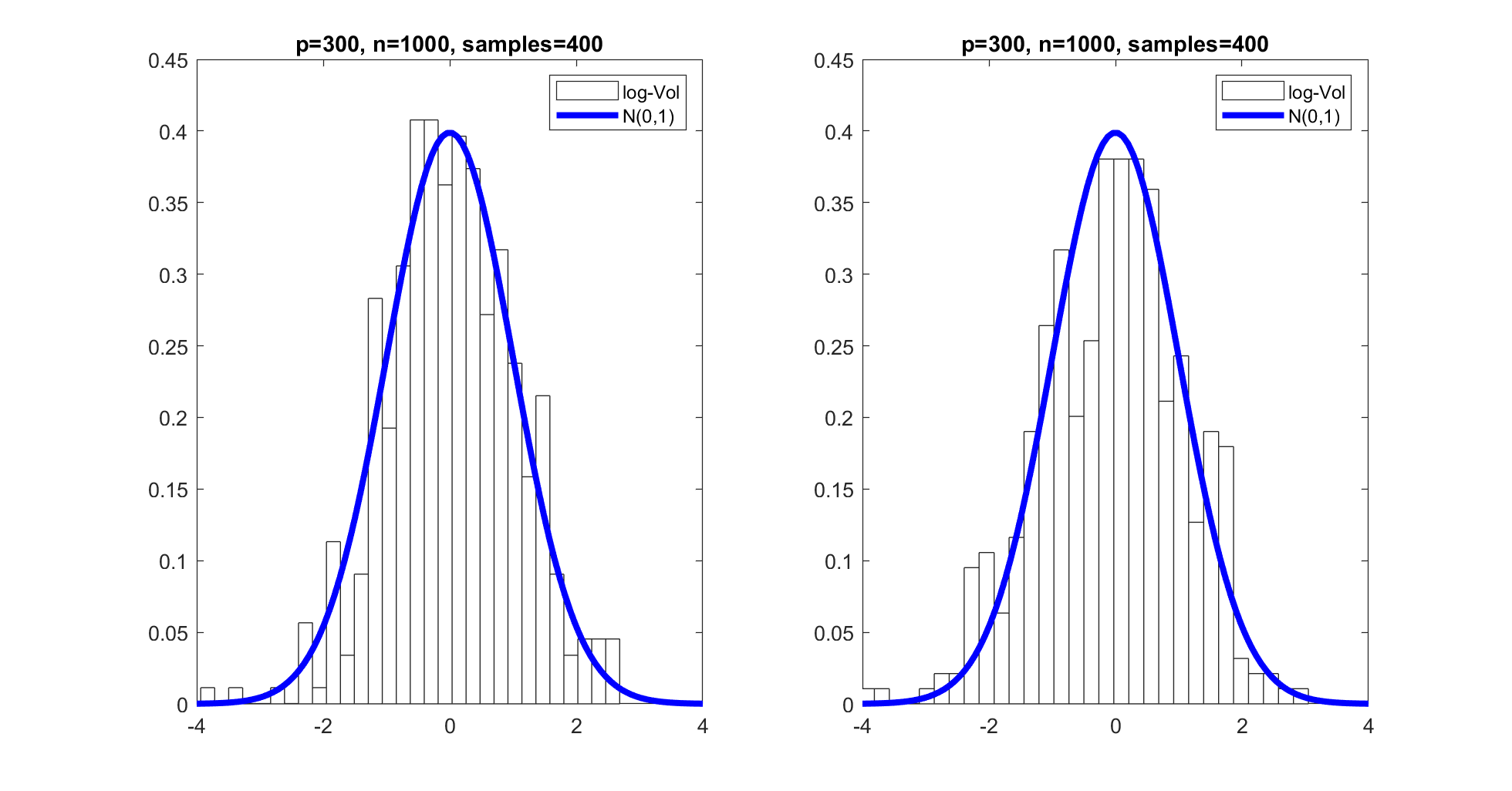
constituting the starting point for our analysis. Since Wn,pW_{n,p} has a representation of order pp independent random variables, it is natural to expect, provided the moments are sufficiently regular, that when appropriately normalized, Wn,pW_{n,p} converges at a speed 1/p1/\sqrt{p} in distribution to a standard Gaussian random variable; see Figure 1 for an illustration.
Refer to caption
Figure 1. Histograms of 400400 simulated log⁡Volp​(Δ⁡(Y1n,…,Ypn))\log\mathrm{Vol}_{p}\left(\Delta(Y_{1}^{n},\ldots,Y_{p}^{n})\right), properly centered and standardized (as in [48]), for p=300p=300 and n=1000n=1000. Left: YinY_{i}^{n} uniformly distributed on the unit sphere. Right: YinY_{i}^{n} with i.i.d. standard normal components.

We find that in a host of natural settings (including Gaussian, beta and beta prime simplices) the dimension nn of the ambient space also contributes to creating Gaussian behavior at a speed much faster than the 1/p1/\sqrt{p} speed predicted by the Berry-Esseen theorem. We prove this by way of a pincer strategy, handling differently the distinct sums on the right-hand side of (6). More concretely, we will focus on random simplices in which the random vectors Y1n,…,YpnY_{1}^{n},\ldots,Y_{p}^{n} are distributed according to a probability measure of the form

(7) μn​(d​s)=1Zn​G​(‖s‖2)​exp⁡(−n​H​(‖s‖2)​d​sCLOSE,\displaystyle\mu^{n}(\mathrm{d}s)=\frac{1}{Z^{n}}G(\|s\|_{2})\exp\left(-nH(\|s\|_{2}\right)\mathrm{d}s,

where ‖s‖2:=(∑i=1nsi2)1/2\|s\|_{2}:=\left(\sum_{i=1}^{n}s_{i}^{2}\right)^{1/2} is the ℓ2\ell_{2}-norm, G,H:[0,∞)→[0,∞)G,H:[0,\infty)\to[0,\infty) are functions satisfying some mild conditions and ZnZ^{n} is a normalization constant. This class of probability measures includes the beta and beta prime models, as well as the Gaussian model (which is obtained after rescaling by 1/n1/\sqrt{n}). Let us briefly outline our results here in the case where p≤θ​np\leq\theta n for a fixed θ<1\theta<1:

  • •

    Consider the random variable

    (8) Wn,pSph:=log⁡Volp​(Δ⁡(Θ1n,…,Θpn))=d−log⁡p!+12​∑j=1p−1log⁡βn−j2,j2.\displaystyle W_{n,p}^{\mathrm{Sph}}:=\log\mathrm{Vol}_{p}\left(\Delta(\Theta_{1}^{n},\ldots,\Theta^{n}_{p})\right)\stackrel{{\scriptstyle\textup{d}}}{{=}}-\log p!+\frac{1}{2}\sum_{j=1}^{p-1}\log\beta_{\frac{n-j}{2},\frac{j}{2}}.

    Using a Fourier-analytic approach, we prove a fast Berry-Esseen bound for the random variable Wn,pSphW_{n,p}^{\mathrm{Sph}}, the word ‘fast’ being used here to indicate that the speed of the bound exceeds 1/p1/\sqrt{p} for pp uniformly bounded away from nn.

  • •

    The next major step in our work is a thin-shell type result for rotationally invariant probability distributions of the form (7). Namely, we show that if X1,X2,X3​…X^{1},X^{2},X^{3}\ldots is a sequence of independent random vectors such that each XiX^{i} takes values in ℝi\mathbb{R}^{i} and is distributed according to μi\mu^{i}, then the sequence of their standardized log-radii

    R~i:=log⁡‖Xi‖2−𝔼⁡[log⁡‖Xi‖2]Var⁡[log⁡‖Xi‖2],i∈ℕ,\displaystyle\tilde{R}^{i}:=\frac{\log\|X^{i}\|_{2}-\mathbb{E}[\log\|X^{i}\|_{2}]}{\sqrt{\mathrm{Var}[\log\|X^{i}\|_{2}]}},\quad i\in\mathbb{N},

    converges in distribution to a standard Gaussian random variable as i→∞i\to\infty. Theorem B below says something stronger however: there is a constant L=L⁡(G,H)∈(0,∞)L=L(G,H)\in(0,\infty) depending on the functions GG and HH but independent of pp and nn such that if X1n,…,XpnX_{1}^{n},\ldots,X^{n}_{p} are independent and identically distributed according to μn\mu^{n}, and R~1n,…,R~pn\tilde{R}^{n}_{1},\ldots,\tilde{R}^{n}_{p} are their associated normalised log-radii, then we have the fast Berry-Esseen bound

    dK​S​(R~1n+…+R~pnp,N)≤L⁡(1p​n+e−c​p),\displaystyle\mathrm{d}_{KS}\left(\frac{\tilde{R}^{n}_{1}+\ldots+\tilde{R}^{n}_{p}}{\sqrt{p}}\,,\,N\right)\leq L\left(\frac{1}{\sqrt{pn}}+\operatorname{e}^{-cp}\right),

    where c>0c>0 is an absolute constant.

  • •

    The two prior results state that both ∑j=1plog⁡Rjn\sum_{j=1}^{p}\log R_{j}^{n} and ∑j=1p−1log⁡βn−j2,j2\sum_{j=1}^{p-1}\log\beta_{\frac{n-j}{2},\frac{j}{2}} are both within certain Kolmogorov-Smirnov distances of Gaussian random variables with certain means and variances. These results may be combined fairly quickly using a triangle inequality for Kolmogorov-Smirnov distances, leading to a proof of Theorem C.

Finally, we drop assumption (7), which is used to relate the distribution of the log-radius of the vectors YinY_{i}^{n} to a Gaussian distribution, and consider more general rotationally invariant random vectors YinY_{i}^{n}. In particular, the log-radius might be in the domain of attraction of an infinite variance stable distribution. Depending on the relation between the tails of the log-radius of YinY_{i}^{n} and the variance of Wn,pSphW_{n,p}^{\mathrm{Sph}} we find that the properly normalized log⁡Volp​(Δ⁡(Y1n,…,Ypn))\log\mathrm{Vol}_{p}\left(\Delta(Y_{1}^{n},\ldots,Y_{p}^{n})\right) either converges to a normal limit, an infinite variance stable limit or a mixture between those two.

Overview of the remainder of the paper

The rest of the paper is structured as follows. In Section 2, we present our main results. First, we present a fast Berry-Esseen theorem for the log-volume of the spherical simplex which is then extended to rotationally invariant random simplices. As a byproduct, we prove a Berry-Esseen type result for the sum of iid random variables whose density resembles the Gaussian density.

In Section 2.3, we provide limit theory for the log-volume of the rotationally invariant random simplices under general conditions, also allowing for very heavy-tailed distributions. Section 2.4 highlights the connection of our findings to random matrix theory. As an application of our results we prove convergence of the logarithmic determinant of an iid standard Gaussian random matrix at speed (logn)−3/2(\log n)^{-3/2}.

Section 3-7 are devoted to the proofs of the results in Section 2. In Section 3, we begin with a careful analysis of random simplices whose vertices are pp points chosen uniformly on the unit sphere in 𝕊n−1\mathbb{S}^{n-1}, culminating in a proof of Theorem A. In Section 4, we introduce our probabilistic approach to the Laplace method, ultimately working towards a proof of Theorem B. Section 5 combines our work in the prior two sections together to prove Theorem C. In the next section, Section 6, we give a short proof of Theorem G, using some of the machinery developed in Section 3. Finally, all results from Section 2.3 are proved in Section 7.

2. Main results

In this section we state our results in full.

2.1. A fast Berry-Esseen theorem for the log-volume of the spherical simplex

Our first result is a Berry-Esseen bound for the spherical random simplex. Here, for integers p≤np\leq n let

(9) W~n,pSph:=Wn,pSph−𝔼⁡[Wn,pSph]Var⁡[Wn,pSph]\displaystyle\widetilde{W}_{n,p}^{\mathrm{Sph}}:=\frac{W_{n,p}^{\mathrm{Sph}}-\mathbb{E}[W_{n,p}^{\mathrm{Sph}}]}{\sqrt{\mathrm{Var}[W_{n,p}^{\mathrm{Sph}}]}}

denote the standardized log-volume of the spherical random simplex associated with pp points chosen independently and uniformly at random from 𝕊n−1\mathbb{S}^{n-1}.

Theorem A.

Let p,n∈ℕp,n\in\mathbb{N} such that p≤np\leq n and W~n,pSph\widetilde{W}_{n,p}^{\mathrm{Sph}} be the normalized log-volume of a spherical simplex. Then there is a universal constant C∈(0,∞)C\in(0,\infty) such that whenever p≥41p\geq 41,

dK​S​(W~n,pSph,N)≤C​θ2n⁡(1−θ)​[log⁡11−θ−θ]3/2,\displaystyle\mathrm{d}_{KS}\left(\widetilde{W}_{n,p}^{\mathrm{Sph}},N\right)\leq\frac{C~\theta^{2}}{n(1-\theta)\left[\log\frac{1}{1-\theta}-\theta\right]^{3/2}},

where θ:=θ⁡(p,n):=p−1n\theta:=\theta(p,n):=\frac{p-1}{n}. In fact, we may take C=28C=28.

We take a moment to unpack the bound in Theorem A by looking at the following easily verified consequences:

  • •

    Fix ϕ∈(0,1)\phi\in(0,1). Using the inequality log⁡11−θ−θ≥θ2/2\log\frac{1}{1-\theta}-\theta\geq\theta^{2}/2 for θ∈[0,1)\theta\in[0,1), it is easily verified that whenever p−1n=θ≤ϕ\frac{p-1}{n}=\theta\leq\phi, we have

    (10) dK​S​(W~n,pSph,N)≤Cϕp−1,\displaystyle\mathrm{d}_{KS}\left(\widetilde{W}_{n,p}^{\mathrm{Sph}},N\right)\leq\frac{C_{\phi}}{p-1},

    where Cϕ:=2​2​C/(1−ϕ)C_{\phi}:=2\sqrt{2}C/(1-\phi).

  • •

    On the other hand, for all p≤np\leq n by setting q:=n−p+1q:=n-p+1 (so that q=n⁡(1−θ)q=n(1-\theta)), we have

    (11) dK​S​(W~n,pSph,N)≤Cq​(log⁡(n/q)−1)3/2.\displaystyle\mathrm{d}_{KS}\left(\widetilde{W}_{n,p}^{\mathrm{Sph}},N\right)\leq\frac{C}{q(\log(n/q)-1)^{3/2}}.

Let us remark here that an analogous result to Theorem A appears in Section 3 of Grote et al. [25, Theorem 3.6], who in contrast to us consider random simplices not having the origin as a fixed vertex. They obtain a similar bound in the case where p−1n\frac{p-1}{n} is bounded away from one, though their bound is weaker in the n−p=o⁡(n)n-p=o(n) case; they obtain C/log1/2⁡(n/q)C/\log^{1/2}(n/q) in the setting of (11).

2.2. A Berry-Esseen theorem for the Laplace method

Our next result concerns the highly Gaussian behavior of the sums of the log-radii. Here we take a moment to give a brief digression on the Laplace method, which states that when gg and hh are suitably regular functions with hh attaining a global minimum at some x0∈(a,b)x_{0}\in(a,b), then we have the asymptotics

(12) ∫abg⁡(x)​e−n​h​(x)​𝑑x=(1+o⁡(1))​2​πn​h′′​(x0)​g​(x0)​exp⁡(−n​h​(x0))\displaystyle\int_{a}^{b}g(x)\operatorname{e}^{-nh(x)}\mathrm{d}x=(1+o(1))\sqrt{\frac{2\pi}{nh^{\prime\prime}(x_{0})}}g(x_{0})\exp(-nh(x_{0}))

as n→∞n\to\infty. See e.g. [6]. The key conceptual point in the Laplace method is that, thanks to the Taylor expansion n​h​(x0+w/n)≈w2​h′′​(x0)/2+O⁡(w3/n)nh(x_{0}+w/\sqrt{n})\approx w^{2}h^{\prime\prime}(x_{0})/2+O(w^{3}/\sqrt{n}), the integral in (12) behaves roughly like a Gaussian integral around x0x_{0}.

Theorem B develops this idea further, stating that when nn is large, random variables whose probability distributions take the form (12) are approximately Gaussian. To set this up, we require some conditions on the functions. For a fixed pair (g,h)(g,h), we consider probability density functions of the form

(13) ρn​(d​x)=1Zn​g​(x)​exp⁡(−n​h​(x))​d​x,n∈ℕ,\displaystyle\rho^{n}(\mathrm{d}x)=\frac{1}{Z^{n}}g(x)\exp\left(-nh(x)\right)\mathrm{d}x,\qquad n\in\mathbb{N},

where the Zn∈(0,∞)Z^{n}\in(0,\infty) are normalization constants, and the ordered pair of functions g,h:[0,∞)→[0,∞)g,h:[0,\infty)\to[0,\infty) is admissible per the following definition.

Definition 2.1.

Let g,h:ℝ→[0,∞)g,h:\mathbb{R}\to[0,\infty) be two functions. We say the pair (g,h)(g,h) is admissible if and only if (a)-(c) hold.

  • (a)

    The density function ρn\rho^{n} is differentiable almost-everywhere, and has a unique maximum at a point x0x_{0} in ℝ\mathbb{R} such that x0x_{0} is a minimum of hh. Moreover, we assume that ρn\rho^{n} is increasing on (−∞,x0](-\infty,x_{0}] and decreasing on [x0,∞)[x_{0},\infty).

  • (b)

    In a neighbourhood [x0−δ,x0+δ][x_{0}-\delta,x_{0}+\delta] of x0x_{0}, hh is twice differentiable. Moreover, if we write

    h⁡(x)=h⁡(x0)+h′′​(x0)​(12​(x−x0)2+r⁡(x))andg⁡(x)=g⁡(x0)​(1+q⁡(x−x0)),\displaystyle h(x)=h(x_{0})+h^{\prime\prime}(x_{0})\left(\frac{1}{2}(x-x_{0})^{2}+r(x)\right)\qquad\text{and}\qquad g(x)=g(x_{0})(1+q(x-x_{0})),

    then we have

    |r⁡(x)|≤14​δ​|x−x0|3and|q⁡(x)|≤14​δ​|x−x0|.\displaystyle|r(x)|\leq\frac{1}{4\delta}|x-x_{0}|^{3}\qquad\text{and}\qquad|q(x)|\leq\frac{1}{4\delta}|x-x_{0}|.
  • (c)

    Outside of this neighborhood, i.e., for each x∈ℝ∖[x0−δ,x0+δ]x\in\mathbb{R}\setminus[x_{0}-\delta,x_{0}+\delta], there exist constants α,c,C∈(0,∞)\alpha,c,C\in(0,\infty) such that

    h⁡(x)≥c​log⁡(1+|x−x0|)andg⁡(x)≤C⁡(1+|x−x0|α).\displaystyle h(x)\geq c\log(1+|x-x_{0}|)\qquad\text{and}\qquad g(x)\leq C(1+|x-x_{0}|^{\alpha}).

As an immediate consequence of Theorem B below, all probability distributions with densities of the form (13) that satisfy Definition 2.1 are in the domain of attraction of the normal law. In particular, they include the Gaussian distribution, the Gamma distribution and the beta distribution.

Our Berry-Esseen theorem for the Laplace method states that when nn is large, the normalized sum of pp independent random variables distributed according to an admissible density ρn\rho^{n} is close in distribution to a standard Gaussian random variable NN.

Theorem B.

For an admissible pair (g,h)(g,h) there is a constant Cg,h∈(0,∞)C_{g,h}\in(0,\infty) and n0∈ℕn_{0}\in\mathbb{N} such that for all n≥n0n\geq n_{0} we have the following: if X1n,…,XpnX_{1}^{n},\ldots,X^{n}_{p} are independent random variables with density ρn\rho^{n} given by (13), then

dK​S​(∑i=1pXin−p​𝔼​[X1n]p​Var​[X1n],N)≤Cg,h​(1p​n+2−p).\displaystyle\mathrm{d}_{KS}\left(\frac{\sum_{i=1}^{p}X^{n}_{i}-p\mathbb{E}[X_{1}^{n}]}{\sqrt{p\,\mathrm{Var}[X_{1}^{n}]}},N\right)\leq C_{g,h}\left(\frac{1}{\sqrt{pn}}+2^{-p}\right).

The value of Theorem B lies in its application to a sort of thin-shell property for a large class of radial densities on ℝn\mathbb{R}^{n}. To this end, we say a pair (G,H)(G,H) of functions G,H:[0,∞)→ℝG,H:[0,\infty)\to\mathbb{R} are radially admissible if the pair (g,h)(g,h) given by

g⁡(s):=G⁡(es)andh⁡(s):=H⁡(es)−s\displaystyle g(s):=G(\operatorname{e}^{s})\qquad\text{and}\qquad h(s):=H(\operatorname{e}^{s})-s

are admissible.

Suppose now for a fixed radially admissible pair (G,H)(G,H) for each n∈ℕn\in\mathbb{N} we have a rotationally invariant probability density on ℝn\mathbb{R}^{n} of the form

(14) μn​(s):=1Zn​G​(‖s‖2)​exp⁡(−n​H​(‖s‖2)),s∈ℝn,\displaystyle\mu^{n}(s):=\frac{1}{Z^{n}}G(\|s\|_{2})\exp\left(-nH(\|s\|_{2})\right),\qquad s\in\mathbb{R}^{n},

where ZnZ^{n} is the normalizing constant. Then by virtue of a straightforward calculation involving the polar integration formula, if XnX^{n} is a random vector distributed according to μn\mu^{n}, then its log radius log⁡‖Xn‖2\log\|X^{n}\|_{2} has the density

1Z~n​G​(er)​exp⁡(−n⁡(H⁡(er)−r))=1Z~n​g​(r)​e−n​h​(r),r∈ℝ,\displaystyle\frac{1}{\widetilde{Z}^{n}}G(\operatorname{e}^{r})\exp\left(-n(H(\operatorname{e}^{r})-r)\right)=\frac{1}{\widetilde{Z}^{n}}\,g(r)\operatorname{e}^{-nh(r)},\qquad r\in\mathbb{R},

on the real line, where Z~n\widetilde{Z}^{n} is again a normalizing constant. This observation is one of the key ingredients in synthesizing Theorem B with Theorem A to obtain the following general result.

Theorem C.

For each radially admissible pair G,HG,H there is a constant CG,H∈(0,∞)C_{G,H}\in(0,\infty) and n0∈ℕn_{0}\in\mathbb{N} such that for all n≥n0n\geq n_{0} we have the following: if Y1n,…,YpnY_{1}^{n},\ldots,Y_{p}^{n} are pp independent random vectors in ℝn\mathbb{R}^{n} distributed according to μn\mu^{n} as it appears in (14), then for Wn,pG,H:=log⁡Volp​(Δ⁡(Y1n,…,Ypn))W^{G,H}_{n,p}:=\log\mathrm{Vol}_{p}\left(\Delta(Y_{1}^{n},\ldots,Y_{p}^{n})\right) it holds that

dK​S​(Wn,pG,H−𝔼⁡[Wn,pG,H]Var⁡[Wn,pG,H],N)≤CG,H​θ2n⁡(1−θ)​[log⁡11−θ−θ]3/2,\displaystyle\mathrm{d}_{KS}\left(\frac{W^{G,H}_{n,p}-\mathbb{E}[W^{G,H}_{n,p}]}{\sqrt{\mathrm{Var}[W^{G,H}_{n,p}]}},N\right)\leq C_{G,H}\frac{\theta^{2}}{n(1-\theta)\left[\log\frac{1}{1-\theta}-\theta\right]^{3/2}},

where θ:=θ⁡(p,n):=p−1n\theta:=\theta(p,n):=\frac{p-1}{n}.

We take a moment to highlight two special cases of Theorem C.

  • •

    The case where G⁡(x)=1G(x)=1 is the identity map and H⁡(x)=x2/2H(x)=x^{2}/2 corresponds to the Gaussian distribution with covariance matrix 1n​In\frac{1}{n}I_{n}, where InI_{n} denotes the n×nn\times n identity matrix.

  • •

    The case where G⁡(x)=1G(x)=1 is the identity map and H⁡(x)=1+ϕ2​log⁡(1+|x|2)H(x)=\frac{1+\phi}{2}\log(1+|x|^{2}) corresponds to the so called Beta prime distribution on ℝn\mathbb{R}^{n} with parameter ν=ϕ​n\nu=\phi n, where ϕ>0\phi>0.

2.3. Fluctuations of the log-volume under general conditions

In this subsection, we work more generally and drop assumption (13), which was used to relate the distribution of the log-radius of the vectors YinY_{i}^{n} to a Gaussian distribution. We consider iid, rotationally invariant random vectors YinY_{i}^{n}, which we collect in the data matrix

(15) 𝐘:=𝐘n:=(Y1n,…,Ypn).\mathbf{Y}:=\mathbf{Y}_{n}:=(Y_{1}^{n},\ldots,Y_{p}^{n})\,.

The main focus is no longer on deriving fast Berry-Esseen bounds for the convergence to the Gaussian distribution. Our goal is to study the asymptotic distribution of log⁡Volp⁡(Δ​𝐘)\log\operatorname{Vol}_{p}\left(\Delta\mathbf{Y}\right) for a wide range of radial laws. For the number of points constituting our simplex, we consider the asymptotic regime

(16) p=pn→∞ and p≤n, as ​n→∞.p=p_{n}\to\infty\quad\text{ and }\quad p\leq n\,,\quad\text{ as }n\to\infty\,.

To simplify notation, we define the random variable R(n)=‖Y1n‖2R_{(n)}=\|Y_{1}^{n}\|_{2} and set R~(n)=log⁡R(n)\widetilde{R}_{(n)}=\log R_{(n)}. For the field (βi/2,j/2)i,j∈ℕ(\beta_{i/2,j/2})_{i,j\in\mathbb{N}} of independent random variables such that βi/2,j/2\beta_{i/2,j/2} is Beta​(i/2,j/2)\text{Beta}(i/2,j/2) distributed, we write β~i/2,j/2=log⁡βi/2,j/2\widetilde{\beta}_{i/2,j/2}=\log\beta_{i/2,j/2}.

Our next result provides conditions on the radius R(n)R_{(n)} under which the fluctuations of the log-volume about its mean are asymptotically Gaussian.

Theorem D (Normal limit).

Under the growth condition (16), consider the data matrix 𝐘\mathbf{Y} defined in (15) with independent and rotationally invariant columns, i.e (3) holds. Assume there exists a sequence of positive constants σn\sigma_{n} such that, as n→∞n\to\infty,

(17) p(𝔼[R~(n)2𝟙{|R~(n)|<σn}]−(𝔼[R~(n)𝟙{|R~(n)|<σn}])2)σn2+14​σn2∑j=1p−1(𝔼[β~n−j2,j22𝟙{|β~n−j2,j2|<2σn}]−(𝔼[β~n−j2,j2𝟙{|β~n−j2,j2|<2σn}])2)→1,\begin{split}&\frac{p\left(\mathbb{E}[\widetilde{R}_{(n)}^{2}\mathds{1}_{\{|\widetilde{R}_{(n)}|<\sigma_{n}\}}]-(\mathbb{E}[\widetilde{R}_{(n)}\mathds{1}_{\{|\widetilde{R}_{(n)}|<\sigma_{n}\}}])^{2}\right)}{\sigma_{n}^{2}}\\ &\quad+\frac{1}{4\sigma_{n}^{2}}\sum_{j=1}^{p-1}\left(\mathbb{E}[\widetilde{\beta}_{\frac{n-j}{2},\frac{j}{2}}^{2}\mathds{1}_{\{|\widetilde{\beta}_{\frac{n-j}{2},\frac{j}{2}}|<2\sigma_{n}\}}]-(\mathbb{E}[\widetilde{\beta}_{\frac{n-j}{2},\frac{j}{2}}\mathds{1}_{\{|\widetilde{\beta}_{\frac{n-j}{2},\frac{j}{2}}|<2\sigma_{n}\}}])^{2}\right)\to 1\,,\end{split}

and

(18) p​ℙ​(|R(n)|≥ε​σn)+∑j=1p−1ℙ⁡(|β~n−j2,j2|≥2​ε​σn)→0,ε>0.p\,\mathbbm{P}(|R_{(n)}|\geq\varepsilon\sigma_{n})+\sum_{j=1}^{p-1}\mathbbm{P}(|\widetilde{\beta}_{\frac{n-j}{2},\frac{j}{2}}|\geq 2\varepsilon\sigma_{n})\to 0\,,\qquad\varepsilon>0\,.

Let (bn)n≥1(b_{n})_{n\geq 1} be a sequence satisfying, as n→∞n\to\infty,

(19) bn=p𝔼[R~(n)𝟙{|R~(n)|<σn}]−log(p!)+12∑j=1p−1𝔼[β~n−j2,j2𝟙{|β~n−j2,j2|<2σn}]+o(σn).b_{n}=p\,\mathbb{E}[\widetilde{R}_{(n)}\mathds{1}_{\{|\widetilde{R}_{(n)}|<\sigma_{n}\}}]-\log(p!)+\frac{1}{2}\sum_{j=1}^{p-1}\mathbb{E}[\widetilde{\beta}_{\frac{n-j}{2},\frac{j}{2}}\mathds{1}_{\{|\widetilde{\beta}_{\frac{n-j}{2},\frac{j}{2}}|<2\sigma_{n}\}}]+o(\sigma_{n})\,.

Then we have

(20) log⁡Volp⁡(Δ​𝐘)−bnσn→dN,n→∞.\frac{\log\operatorname{Vol}_{p}(\Delta\mathbf{Y})-b_{n}}{\sigma_{n}}\stackrel{{\scriptstyle\rm d}}{{\rightarrow}}N\,,\qquad n\to\infty\,.

Theorem D characterises the distributions of radii such that the logarithmic volume satisfies a central limit theorem. In fact, since Petrov’s [49] infinite smallness condition is always satisfied in our model, a slightly stronger result holds under the assumptions of Theorem D and a sequence of positive constants σn\sigma_{n}. Namely, the existence of a non-random sequence (bn)(b_{n}) such that (20) holds is equivalent to (σn)(\sigma_{n}) satsifying (17) and (18). If (17) and (18) hold, we may choose bnb_{n} as in (19).

Our next result shows that the logarithmic volume can also have an α\alpha-stable limit. In particular, this is the case when R~(n)\widetilde{R}_{(n)} has power law tails with index α<2\alpha<2. To the best of our knowledge, the most general setting in which the limiting distribution of the log-volume (or equivalently the log-determinant) was derived was in [9, 59] who assumed that the entries of 𝐘\mathbf{Y} possess a finite fourth moment, which is the typical assumption in papers on linear spectral statistics. We refer to [8, 18, 27, 28, 21, 11, 29, 30] for collections of results which show the stark differences in the asymptotic behavior under infinite fourth moments.

In order to present our stable limit theorem, we introduce the auxiliary sequence

(21) ωn2:=−12​log⁡n−p+1n−p22​n​(p+1),n≥1,\omega_{n}^{2}:=-\frac{1}{2}\log\frac{n-p+1}{n}-\frac{p^{2}}{2n(p+1)}\,,\qquad n\geq 1\,,

which one may interpret as the critical variance sequence.

Theorem E (α\alpha-stable limit).

Under the growth condition (16), consider the data matrix 𝐘\mathbf{Y} defined in (15) with independent and rotationally invariant rows, i.e (3) holds. For some α∈(0,2)\alpha\in(0,2) and c1,c2≥0c_{1},c_{2}\geq 0 with c1+c2>0c_{1}+c_{2}>0, assume that there exists a sequence of positive constants σn\sigma_{n} such that, as n→∞n\to\infty, ωn/σn→0\omega_{n}/\sigma_{n}\to 0 and

(22) pℙ(σn−1R~(n)≤−x)→c1x−α,pℙ(σn−1R~(n)>x)→c2x−α,x>0, and\displaystyle p\,\mathbbm{P}(\sigma_{n}^{-1}\widetilde{R}_{(n)}\leq-x)\to c_{1}x^{-\alpha}\,,\quad p\,\mathbbm{P}(\sigma_{n}^{-1}\widetilde{R}_{(n)}>x)\to c_{2}x^{-\alpha}\,,\qquad x>0\,,\text{ and}
(23) limε→0lim supn→∞pσn2(𝔼[R~(n)2𝟙{|R~(n)|<εσn}]−(𝔼[R~(n)𝟙{|R~(n)|<εσn}])2)=0.\displaystyle\lim_{\varepsilon\to 0}\limsup_{n\to\infty}\frac{p}{\sigma_{n}^{2}}\left(\mathbb{E}[\widetilde{R}_{(n)}^{2}\mathds{1}_{\{|\widetilde{R}_{(n)}|<\varepsilon\sigma_{n}\}}]-(\mathbb{E}[\widetilde{R}_{(n)}\mathds{1}_{\{|\widetilde{R}_{(n)}|<\varepsilon\sigma_{n}\}}])^{2}\right)=0\,.

Set an=σn−1𝔼[R~(n)𝟙{|R~(n)|<σn}]a_{n}=\sigma_{n}^{-1}\mathbb{E}[\widetilde{R}_{(n)}\mathds{1}_{\{|\widetilde{R}_{(n)}|<\sigma_{n}\}}] and let (bn)n≥1(b_{n})_{n\geq 1} be a sequence satisfying

bn=−log⁡(p!)+12​∑j=1p−1𝔼⁡[β~n−j2,j2]+p​σn​(an+∫−∞∞x1+x2​𝑑ℙ​(R~(n)≤σn​(x+an)))+o⁡(σn).b_{n}=-\log(p!)+\frac{1}{2}\sum_{j=1}^{p-1}\mathbb{E}[\widetilde{\beta}_{\frac{n-j}{2},\frac{j}{2}}]+p\sigma_{n}\left(a_{n}+\int_{-\infty}^{\infty}\frac{x}{1+x^{2}}\,d\mathbbm{P}(\widetilde{R}_{(n)}\leq\sigma_{n}(x+a_{n}))\right)+o(\sigma_{n})\,.

Then we have the following weak convergence to an α\alpha-stable limit:

log⁡Volp⁡(Δ​𝐘)−bnσn→dZα,n→∞.\frac{\log\operatorname{Vol}_{p}\left(\Delta\mathbf{Y}\right)-b_{n}}{\sigma_{n}}\stackrel{{\scriptstyle\rm d}}{{\rightarrow}}Z_{\alpha}\,,\qquad n\to\infty\,.

The limit random variable Zα=Zα​(c1,c2)Z_{\alpha}=Z_{\alpha}(c_{1},c_{2}) has the characteristic function

(24) 𝔼⁡[ei​t​Zα]={exp⁡{α⁡(c1+c2)​Γ​(−α)​cos⁡(π​α2)​|t|α​(1−i​η​tan⁡(π​α2)​sign⁡(t))},if ​α≠1,exp⁡{−(c1+c2)​π2​|t|​(1+i​η​2π​sign⁡(t)​log​|t|)},if ​α=1,\mathbb{E}[\operatorname{e}^{{\rm i}tZ_{\alpha}}]=\left\{\begin{array}[]{ll}\exp\left\{\alpha(c_{1}+c_{2})\Gamma(-\alpha)\cos(\frac{\pi\alpha}{2})|t|^{\alpha}\big(1-{\rm i}\eta\tan(\frac{\pi\alpha}{2})\operatorname{sign}(t)\big)\right\}\,,&\mbox{if }\alpha\neq 1,\\ \exp\left\{-(c_{1}+c_{2})\frac{\pi}{2}|t|\big(1+{\rm i}\eta\frac{2}{\pi}\operatorname{sign}(t)\log|t|\big)\right\}\,,&\mbox{if }\alpha=1,\end{array}\right.

where η=(c2−c1)/(c1+c2)\eta=(c_{2}-c_{1})/(c_{1}+c_{2}).

Finally, there is an interesting mixed case, when the variances of the two sums on the right-hand side of (6) are of the same order.

Theorem F (mixed limit).

Under the growth condition (16), consider the data matrix 𝐘\mathbf{Y} defined in (15) with independent and rotationally invariant rows, i.e (3) holds. For some α∈(0,2)\alpha\in(0,2) and c1,c2≥0c_{1},c_{2}\geq 0 with c1+c2>0c_{1}+c_{2}>0, assume that there exists a sequence of positive constants σn\sigma_{n} such that, as n→∞n\to\infty, ωn/σn→q∈(0,∞)\omega_{n}/\sigma_{n}\to q\in(0,\infty) and

(25) pℙ(σn−1R~(n)≤−x)→c1x−α,pℙ(σn−1R~(n)>x)→c2x−α,x>0, and\displaystyle p\,\mathbbm{P}(\sigma_{n}^{-1}\widetilde{R}_{(n)}\leq-x)\to c_{1}x^{-\alpha}\,,\quad p\,\mathbbm{P}(\sigma_{n}^{-1}\widetilde{R}_{(n)}>x)\to c_{2}x^{-\alpha}\,,\qquad x>0\,,\text{ and}
(26) limε→0lim supn→∞pσn2(𝔼[R~(n)2𝟙{|R~(n)|<εσn}]−(𝔼[R~(n)𝟙{|R~(n)|<εσn}])2)=0.\displaystyle\lim_{\varepsilon\to 0}\limsup_{n\to\infty}\frac{p}{\sigma_{n}^{2}}\left(\mathbb{E}[\widetilde{R}_{(n)}^{2}\mathds{1}_{\{|\widetilde{R}_{(n)}|<\varepsilon\sigma_{n}\}}]-(\mathbb{E}[\widetilde{R}_{(n)}\mathds{1}_{\{|\widetilde{R}_{(n)}|<\varepsilon\sigma_{n}\}}])^{2}\right)=0\,.

Set an=σn−1𝔼[R~(n)𝟙{|R~(n)|<σn}]a_{n}=\sigma_{n}^{-1}\mathbb{E}[\widetilde{R}_{(n)}\mathds{1}_{\{|\widetilde{R}_{(n)}|<\sigma_{n}\}}] and let (bn)n≥1(b_{n})_{n\geq 1} be a sequence satisfying

bn=−log⁡(p!)+12​∑j=1p−1𝔼⁡[β~n−j2,j2]+p​σn​(an+∫−∞∞x1+x2​dℙ​(R~(n)≤σn​(x+an)))+o⁡(σn).\begin{split}b_{n}&=-\log(p!)+\frac{1}{2}\sum_{j=1}^{p-1}\mathbb{E}[\widetilde{\beta}_{\frac{n-j}{2},\frac{j}{2}}]+p\sigma_{n}\left(a_{n}+\int_{-\infty}^{\infty}\frac{x}{1+x^{2}}\,d\mathbbm{P}(\widetilde{R}_{(n)}\leq\sigma_{n}(x+a_{n}))\right)+o(\sigma_{n})\,.\end{split}

Then we have

log⁡Volp⁡(Δ​𝐘)−bnσn→dq​N+Zα,n→∞,\frac{\log\operatorname{Vol}_{p}\left(\Delta\mathbf{Y}\right)-b_{n}}{\sigma_{n}}\stackrel{{\scriptstyle\rm d}}{{\rightarrow}}q\,N+Z_{\alpha}\,,\qquad n\to\infty\,,

where Zα=Zα​(c1,c2)Z_{\alpha}=Z_{\alpha}(c_{1},c_{2}) has the characteristic function (24).

2.4. The random matrix perspective

While we have discussed our results so far from the perspective of the volumes of random simplices, the framework we considered is intimately related to the determinants of random matrices. Indeed, we saw in (2) that the volume of a simplex with vertices Y1n,…,YpnY^{n}_{1},\ldots,Y^{n}_{p} in ℝn\mathbb{R}^{n} may be expressed in terms of a determinant. Developing this equation slightly, we may write

(27) Volp​(Δ⁡(Y1n,…,Ypn))=Volp​(Δ​𝐘)=1p!​det⁡(𝐘⊤​𝐘),\displaystyle\mathrm{Vol}_{p}\left(\Delta(Y^{n}_{1},\ldots,Y^{n}_{p})\right)=\mathrm{Vol}_{p}\left(\Delta\mathbf{Y}\right)=\frac{1}{p!}\sqrt{\mathrm{det}(\mathbf{Y}^{\top}\mathbf{Y})},

where 𝐘:=𝐘n\mathbf{Y}:=\mathbf{Y}_{n} is the n×pn\times p matrix whose columns are given by Y1n,…,YpnY^{n}_{1},\ldots,Y^{n}_{p}. In particular, we may invert the relation

log⁡det⁡(𝐘⊤​𝐘)=2​(log⁡Vol⁡(Δ​𝐘)+log⁡p!)\displaystyle\log\mathrm{det}(\mathbf{Y}^{\top}\mathbf{Y})=2\left(\log\mathrm{Vol}(\Delta\mathbf{Y})+\log p!\right)

to obtain various statements about the log-determinants of random matrices 𝐘⊤\mathbf{Y}^{\top} whose columns are rotationally invariant random vectors. We remark that for our decomposition in (1.2) it is important that the rows of 𝐘\mathbf{Y} are independent rotationally invariant random vectors. If instead the columns of 𝐘\mathbf{Y} were rotationally invariant, one cannot separate the radius from the direction as in (1.2) even though 𝐘⊤​𝐘\mathbf{Y}^{\top}\mathbf{Y} and 𝐘𝐘⊤\mathbf{Y}\mathbf{Y}^{\top} have the same non-zero eigenvalues. The phenomenon that the roles of rows and columns are not interchangeable is illustrated in Figure 2.

Refer to caption
Figure 2. Histograms of 300300 simulated log⁡Volp​(Δ​𝐘)\log\mathrm{Vol}_{p}\left(\Delta\mathbf{Y}\right), properly centered and standardized (as in [48]), for p=300p=300 and n=1000n=1000. Left: multivariate t−t-distributed rows of 𝐘\mathbf{Y} with 60 degrees of freedom. Right: multivariate t−t-distributed columns of 𝐘\mathbf{Y} with 60 degrees of freedom.

Before discussing the applications of our results to the determinants of random matrices, we take a moment to highlight just a single result from the large body of work on the asymptotic distribution of the logarithms of such determinants [24, 55, 9, 59, 48]. Namely, Nyugen and Vu [47] consider the log-determinant of an n×nn\times n random matrix AnA^{n} with independent and identically distributed entries with zero mean, unit variance and finite fourth moment. They show that, as n→∞n\to\infty,

dK​S(log⁡|det(An)|−12​log⁡(n−1)!12​log⁡n,N)=(logn)−1/3+o(1).\displaystyle\mathrm{d}_{KS}\left(\frac{\log|\det(A^{n})|-\frac{1}{2}\log(n-1)!}{\sqrt{\frac{1}{2}\log n}},N\right)=(\log n)^{-1/3+o(1)}\,.

Nguyen and Vu speculate that (logn)−1/3(\log n)^{-1/3} could be the optimal rate of convergence for such a theorem, though suggest that this could be potentially improved to (logn)−1/2(\log n)^{-1/2} with a finer correction for the expectation of the log determinant. It transpires that when the entries are further assumed to be independent standard Gaussians, the rate of convergence can be improved to (logn)−3/2(\log n)^{-3/2}. To this end, we require estimates on the mean and variance of log⁡|det(An)|\log|\det(A^{n})| that are fine up to constant order. To this end, let γ:=limn→∞(∑k=1n1/k−log⁡n)\gamma:=\lim_{n\to\infty}\left(\sum_{k=1}^{n}1/k-\log n\right) denote the Euler-Mascheroni constant, and define the constants

(28) c0:=−γ2−12​∫0∞(12−1ζ+1eζ−1)​1eζ/2−1​𝑑ζ\displaystyle c_{0}:=-\frac{\gamma}{2}-\frac{1}{2}\int_{0}^{\infty}\left(\frac{1}{2}-\frac{1}{\zeta}+\frac{1}{\operatorname{e}^{\zeta}-1}\right)\frac{1}{\operatorname{e}^{\zeta/2}-1}\mathrm{d}\zeta

and

(29) c1:=γ2+14​∫0∞(12−1ζ+1eζ−1)​ζeζ/2−1​𝑑ζ.\displaystyle c_{1}:=\frac{\gamma}{2}+\frac{1}{4}\int_{0}^{\infty}\left(\frac{1}{2}-\frac{1}{\zeta}+\frac{1}{\operatorname{e}^{\zeta}-1}\right)\frac{\zeta}{\operatorname{e}^{\zeta/2}-1}\mathrm{d}\zeta.

We believe the following result to be new.

Theorem G.

Let n∈ℕn\in\mathbb{N} and AnA^{n} be an n×nn\times n matrix whose entries are independent standard Gaussian random variables. Then, we have

dK​S​(log⁡|det(An)|−(12​log⁡(n−1)!+c0)12​log⁡n+c1,N)≤Clog3/2⁡n,\displaystyle\mathrm{d}_{KS}\left(\frac{\log|\det(A^{n})|-(\frac{1}{2}\log(n-1)!+c_{0})}{\sqrt{\frac{1}{2}\log n+c_{1}}},N\right)\leq\frac{C}{\log^{3/2}n},

where C∈(0,∞)C\in(0,\infty) is an absolute constant.

Theorem G is proved directly in Section 6. A weaker version of Theorem G, without explicit estimates for the mean and variance of log⁡|det(An)|\log|\det(A^{n})| is actually an indirect consequence of a more general result concerning the log-determinants of random matrices whose columns are distributed according to a rotationally invariant probabillity density μn\mu^{n} on ℝn\mathbb{R}^{n}. Namely, the following result is an immediate corollary of Theorem C, using (27) to restate the result in terms of determinants of random matrices rather than volumes of random simplices.

Theorem H.

Let An,pA^{n,p} be an n×pn\times p matrix whose pp columns Y1n,…,YpnY_{1}^{n},\ldots,Y_{p}^{n} are independent and identically distributed according to a probability density of the form μn\mu^{n}, with μn\mu^{n} as in (14) and (G,H)(G,H) a radially admissible pair. Then there is a constant CG,H∈(0,∞)C_{G,H}\in(0,\infty) such that

dK​S​(logdet((An,p)⊤An,p))−𝔼[logdet((An,p)⊤An,p)]Var[logdet((An,p)⊤An,p)],N)≤CG,H​θ2n⁡(1−θ)​[log⁡11−θ−θ]3/2,\displaystyle\mathrm{d}_{KS}\left(\frac{\log\det\left((A^{n,p})^{\top}A^{n,p}\right))-\mathbb{E}\left[\log\det\left((A^{n,p})^{\top}A^{n,p}\right)\right]}{\sqrt{\mathrm{Var}[\log\det\left((A^{n,p})^{\top}A^{n,p}\right)]}},N\right)\leq C_{G,H}\frac{\theta^{2}}{n(1-\theta)\left[\log\frac{1}{1-\theta}-\theta\right]^{3/2}},

where θ:=θ⁡(p,n):=p−1n\theta:=\theta(p,n):=\frac{p-1}{n}.

That completes the section on random matrices.

3. Extremely Gaussian behavior for spherical random simplices

The chief focus of this section will be in analyzing the Gaussian behavior of the log-volume of random simplices whose vertices are uniformly distributed on the unit sphere. We begin in the next section by discussing the polar integration formula and radial laws.

3.1. The polar integration formula and radial laws

Throughout we will use the following polar integration formula. Let f:ℝn→[0,∞)f:\mathbb{R}^{n}\to[0,\infty) be an integrable function on ℝn\mathbb{R}^{n} depending only on the Euclidean norm, in the sense that f​(s)=f~​(‖s‖2)f(s)=\widetilde{f}(\|s\|_{2}) for some f~:[0,∞)→[0,∞)\widetilde{f}:[0,\infty)\to[0,\infty). Then the polar integration formula states that

(30) ∫ℝnf⁡(s)​d​s=2​πn/2Γ⁡(n/2)​∫0∞rn−1​f~​(r)​d​r.\displaystyle\int_{\mathbb{R}^{n}}f(s)\,\textup{d}s=\frac{2\pi^{n/2}}{\Gamma(n/2)}\int_{0}^{\infty}r^{n-1}\widetilde{f}(r)\,\textup{d}r.

Given a Borel subset AA of [0,∞)[0,\infty), define the Borel subset radn​(A)\mathrm{rad}_{n}(A) of ℝn\mathbb{R}^{n} by setting

radn​(A):={s∈ℝn:‖s‖2∈A}.\displaystyle\mathrm{rad}_{n}(A):=\{s\in\mathbb{R}^{n}\,:\,\|s\|_{2}\in A\}.

Given any probability distribution μ\mu on ℝn\mathbb{R}^{n}, we define the radial law ν\nu associated with μ\mu to be the probability measure on [0,∞)[0,\infty) defined by setting

ν⁡(A):=μ⁡(radn​(A)).\displaystyle\nu\left(A\right):=\mu\left(\mathrm{rad}_{n}(A)\right).

We now record the following simple lemma on the radial laws of rotationally invariant distributions of standard form.

Lemma 3.1.

Let μn\mu_{n} be a rotationally invariant probability distribution on ℝn\mathbb{R}^{n} of the form

μn​(d​s)=Cn​g​(‖s‖2)​e−n​h​(‖s‖2)​d​s.\displaystyle\mu_{n}(\textup{d}s)=C_{n}g(\|s\|_{2})\operatorname{e}^{-nh(\|s\|_{2})}\textup{d}s.

where g,h:[0,∞)→[0,∞)g,h:[0,\infty)\to[0,\infty) are measurable functions. Then the radial law νn\nu_{n} associated with μn\mu_{n} is given by

νn​(d​r)=2​πn/2​CnΓ⁡(n/2)​rn−1​g​(r)​e−n​h​(r)​d​r.\displaystyle\nu_{n}(\textup{d}r)=\frac{2\pi^{n/2}C_{n}}{\Gamma(n/2)}r^{n-1}g(r)\operatorname{e}^{-nh(r)}\textup{d}r.
Proof.

Let AA be a Borel subset of [0,∞)[0,\infty). Then

νn​(A)=μn​(radn​(A))=∫ℝnf⁡(s)​d​s,\displaystyle\nu_{n}(A)=\mu_{n}\left(\mathrm{rad}_{n}(A)\right)=\int_{\mathbb{R}^{n}}f(s)\,\textup{d}s,

where for s∈ℝns\in\mathbb{R}^{n}, f⁡(s):=𝟙radn​(A)​(s)​Cn​g​(‖s‖2)​e−n​h​(‖s‖2)f(s):=\mathds{1}_{\mathrm{rad}_{n}(A)}(s)C_{n}g(\|s\|_{2})\operatorname{e}^{-nh(\|s\|_{2})}. The result follows after applying (30). ∎

3.2. Miles’ identity

Integral to our analysis is the distributional identity (5) which is a consequence of the following proposition, which was recently given in Grote, Kabluchko and Thäle [25, Theorem 2.4(d)], though similar identities date back (at least) to Miles [45].

Proposition 3.2.

Let Θ1n,…,Θpn\Theta^{n}_{1},\ldots,\Theta^{n}_{p} be points chosen independently and uniformly from the Euclidean unit sphere 𝕊n−1\mathbb{S}^{n-1} in ℝn\mathbb{R}^{n}. Then we have the following identity in law

(31) Volp⁡(Δ⁡(Θ1n,…,Θpn))=d1p!​(∏j=1p−1βn−j2,j2)1/2,\displaystyle\operatorname{Vol}_{p}\left(\Delta(\Theta^{n}_{1},\ldots,\Theta^{n}_{p})\right)\stackrel{{\scriptstyle\textup{d}}}{{=}}\frac{1}{p!}\left(\prod_{j=1}^{p-1}\beta_{\frac{n-j}{2},\frac{j}{2}}\right)^{1/2}\,,

where {βn−j2,j2:j=1,…,p−1}\left\{\beta_{\frac{n-j}{2},\frac{j}{2}}:j=1,\ldots,p-1\right\} is a collection of independent random variables such that βn−j2,j2\beta_{\frac{n-j}{2},\frac{j}{2}} is beta distributed with parameters (n−j2,j2)\left(\frac{n-j}{2},\frac{j}{2}\right).

It is immediate from Proposition 3.2 that the log-volume of the spherical random simplex may be written as

(32) Wn,pSph:=log⁡Volp​Δ​(Θ1n,…,Θpn)=d−log⁡p!+12​∑j=1p−1log⁡β(n−j)/2,j/2.\displaystyle W_{n,p}^{\mathrm{Sph}}:=\log\mathrm{Vol}_{p}\Delta\left(\Theta_{1}^{n},\ldots,\Theta^{n}_{p}\right)\stackrel{{\scriptstyle\textup{d}}}{{=}}-\log p!+\frac{1}{2}\sum_{j=1}^{p-1}\log\beta_{(n-j)/2,j/2}.

3.3. Polygamma functions

For complex ζ\zeta with positive real part, let Γ⁡(ζ):=∫0∞uζ−1​e−u​d​u\Gamma(\zeta):=\int_{0}^{\infty}u^{\zeta-1}\operatorname{e}^{-u}\,\textup{d}u be the gamma function. Then the kk-th polygamma function is given by

(33) ψk​(ζ):=dk+1d​ζk+1​log⁡Γ⁡(ζ),ζ∈ℂ,Re⁡(ζ)>0.\displaystyle\psi_{k}(\zeta):=\frac{\mathrm{d}^{k+1}}{\mathrm{d}\zeta^{k+1}}\log\Gamma(\zeta)\,,\qquad\zeta\in\mathbb{C},\,\mathrm{Re}(\zeta)>0.

The zeroth{}^{\text{th}} polygamma function ψ0\psi_{0}, better known as the digamma function, has the following integral representation

(34) ψ0​(ζ):=∫0∞(e−tt−e−ζ​t1−e−t)​d​t,ζ∈ℂ,Re⁡(ζ)>0,\displaystyle\psi_{0}(\zeta):=\int_{0}^{\infty}\left(\frac{\operatorname{e}^{-t}}{t}-\frac{\operatorname{e}^{-\zeta t}}{1-\operatorname{e}^{-t}}\right)\,\textup{d}t,\qquad\zeta\in\mathbb{C},\,\mathrm{Re}(\zeta)>0,

due to Gauss (see e.g. [43, Section 1.4]). By differentiating through Gauss’ integral representation (34) for k≥1k\geq 1 we have

(35) ψk​(ζ)=(−1)k−1​∫0∞tk​e−ζ​t1−e−t​𝑑t.\displaystyle\psi_{k}(\zeta)=(-1)^{k-1}\int_{0}^{\infty}\frac{t^{k}e^{-\zeta t}}{1-e^{-t}}\mathrm{d}t.

A simple calculation involving the gamma integral tells us that we have the sandwich inequality

(36) (k−1)!ζk+k!2​ζk+1≤ψk​(ζ)≤(k−1)!ζk+k!ζk+1k≥1,ζ∈[1/2,∞)\displaystyle\frac{(k-1)!}{\zeta^{k}}+\frac{k!}{2\zeta^{k+1}}\leq\psi_{k}(\zeta)\leq\frac{(k-1)!}{\zeta^{k}}+\frac{k!}{\zeta^{k+1}}\qquad k\geq 1,\zeta\in[1/2,\infty)

Finally, we note from (35) that for ζ\zeta in ℂ\mathbb{C} with Re⁡(ζ)>0\mathrm{Re}(\zeta)>0 we have |ψk​(ζ)|≤|ψk​(Re⁡(ζ))||\psi_{k}(\zeta)|\leq|\psi_{k}(\mathrm{Re}(\zeta))|. In particular, with Ck=(k−1)!+2​k!C_{k}=(k-1)!+2k! we may extract from (36) the upper bound

(37) |ψk​(ζ)|≤CkRe​(ζ)kζ∈ℂ,Re⁡(ζ)≥1/2.\displaystyle|\psi_{k}(\zeta)|\leq\frac{C_{k}}{\mathrm{Re}(\zeta)^{k}}\qquad\zeta\in\mathbb{C},\mathrm{Re}(\zeta)\geq 1/2.

3.4. Moments of log-beta random variables

In this subsection, we provide all moments of the log-beta random variables in terms of combinatorial expressions involving the polygamma functions. To this end, we need the one-dimensional Faà di Bruno formula (see, e.g., [34] for this and its multivariate form). To set this up, recall that a partition of {1,…,k}\{1,\ldots,k\} is a collection of disjoint subsets (called blocks) of {1,…,k}\{1,\ldots,k\} whose union is equal to {1,…,k}\{1,\ldots,k\}. Let 𝒫k\mathcal{P}_{k} be the collection of set partitions of {1,…,k}\{1,\ldots,k\}. For partitions π\pi in 𝒫k\mathcal{P}_{k}, let #​π\#\pi denote the number of blocks in π\pi. For a block Γ\Gamma of some π\pi, let #​Γ\#\Gamma denote the number of elements of {1,…,k}\{1,\ldots,k\} contained in Γ\Gamma.

Namely, if k∈ℕk\in\mathbb{N} and f,g:ℝ→ℝf,g:\mathbb{R}\to\mathbb{R} are kk times differentiable functions, then Faà di Bruno’s formula states that the kk-th derivative of the composition f∘gf\circ g is given by

dkd​ζk​f​(g⁡(ζ))=∑π∈𝒫kf(#​j)​(g⁡(ζ))​∏Γ∈πg(#​Γ)​(ζ),\displaystyle\frac{\mathrm{d}^{k}}{\mathrm{d}\zeta^{k}}f\left(g(\zeta)\right)=\sum_{\pi\in\mathcal{P}_{k}}f^{(\#j)}\left(g(\zeta)\right)\prod_{\Gamma\in\pi}g^{(\#\Gamma)}(\zeta),

where for j∈ℕj\in\mathbb{N}, f(j)f^{(j)} and g(j)g^{(j)} denote the jj-th derivatives of ff and gg respectively. We note that in particular, when f⁡(ζ)=eζf(\zeta)=\operatorname{e}^{\zeta}, we have

(38) dkd​ζkeg⁡(ζ)=eg⁡(ζ)∑π∈𝒫k∏Γ∈πg(#​Γ)(ζ).\displaystyle\frac{\mathrm{d}^{k}}{\mathrm{d}\zeta^{k}}\operatorname{e}^{g(\zeta)}=\operatorname{e}^{g(\zeta)}\sum_{\pi\in\mathcal{P}_{k}}\prod_{\Gamma\in\pi}g^{(\#\Gamma)}(\zeta).

We are now equipped to give a combinatorial representation for the moments of the logarithm of a beta random variable in terms of set partitions and the polygamma functions.

Lemma 3.3.

Let βζ,η\beta_{\zeta,\eta} be beta distributed with parameters (ζ,η)(\zeta,\eta). Then

𝔼⁡[(log⁡βζ,η)k]=∑π∈𝒫k∏Γ∈πq#​Γ​(ζ,η),\displaystyle\mathbb{E}\Big[\left(\log\beta_{\zeta,\eta}\right)^{k}\Big]=\sum_{\pi\in\mathcal{P}_{k}}\prod_{\Gamma\in\pi}q_{\#\Gamma}(\zeta,\eta),

where for integers j∈ℕj\in\mathbb{N}, qj​(ζ,η):=ψj−1​(ζ)−ψj−1​(ζ+η)q_{j}(\zeta,\eta):=\psi_{j-1}(\zeta)-\psi_{j-1}(\zeta+\eta).

Proof.

First we make the observation that

𝔼⁡[log⁡βζ,η]\displaystyle\mathbb{E}[\log\beta_{\zeta,\eta}] =Γ⁡(ζ+η)Γ⁡(ζ)​Γ​(η)​∫01(log⁡s)k​sζ−1​(1−s)η−1​𝑑s\displaystyle=\frac{\Gamma(\zeta+\eta)}{\Gamma(\zeta)\Gamma(\eta)}\int_{0}^{1}\left(\log s\right)^{k}~s^{\zeta-1}(1-s)^{\eta-1}\mathrm{d}s
=Γ⁡(ζ+η)Γ⁡(ζ)​Γ​(η)​∫01dkd​ζk​sζ−1​(1−s)η−1​𝑑s.\displaystyle=\frac{\Gamma(\zeta+\eta)}{\Gamma(\zeta)\Gamma(\eta)}\int_{0}^{1}\frac{\mathrm{d}^{k}}{\mathrm{d}\zeta^{k}}s^{\zeta-1}(1-s)^{\eta-1}\mathrm{d}s.

In particular, by taking the derivative outside the integral, we may write

𝔼⁡[log⁡βζ,η]=e−g⁡(ζ)⁡dkd​ζk​eg⁡(ζ),\displaystyle\mathbb{E}[\log\beta_{\zeta,\eta}]=\operatorname{e}^{-g(\zeta)}\frac{\mathrm{d}^{k}}{\mathrm{d}\zeta^{k}}\operatorname{e}^{g(\zeta)},

where g⁡(ζ):=log⁡Γ⁡(ζ)−log⁡Γ⁡(ζ+η)g(\zeta):=\log\Gamma(\zeta)-\log\Gamma(\zeta+\eta). The result follows by using (38) and the definition (33) of the polygamma functions. ∎

Our second lemma gives us the centered moments.

Lemma 3.4.

Let k∈ℕk\in\mathbb{N} and 𝒬k\mathcal{Q}_{k} be the collection of set partitions of {1,…,k}\{1,\ldots,k\} containing no singletons. Assume that βζ,η\beta_{\zeta,\eta} is beta distributed with parameters (ζ,η)(\zeta,\eta). Then

𝔼⁡[(log⁡βζ,η−𝔼⁡[log⁡βζ,η])k]=∑π∈𝒬k∏Γ∈πq#​Γ​(ζ,η),\displaystyle\mathbb{E}\Big[\left(\log\beta_{\zeta,\eta}-\mathbb{E}[\log\beta_{\zeta,\eta}]\right)^{k}\Big]=\sum_{\pi\in\mathcal{Q}_{k}}\prod_{\Gamma\in\pi}q_{\#\Gamma}(\zeta,\eta),

where for integers j∈ℕj\in\mathbb{N}, qj​(ζ,η):=ψj−1​(ζ)−ψj−1​(ζ+η)q_{j}(\zeta,\eta):=\psi_{j-1}(\zeta)-\psi_{j-1}(\zeta+\eta).

Proof.

We begin with the observation that

𝔼⁡[(log⁡βζ,η−𝔼⁡[log⁡βζ,η])k]=∑𝒮⊆{1,…,k}(−1)k−#​𝒮​q1k−#​𝒮​𝔼​[(log⁡βζ,η)#​𝒮],\displaystyle\mathbb{E}\Big[\left(\log\beta_{\zeta,\eta}-\mathbb{E}[\log\beta_{\zeta,\eta}]\right)^{k}\Big]=\sum_{\mathcal{S}\subseteq\{1,\ldots,k\}}(-1)^{k-\#\mathcal{S}}q_{1}^{k-\#\mathcal{S}}\mathbb{E}[(\log\beta_{\zeta,\eta})^{\#\mathcal{S}}],

where we wrote qj:=qj​(ζ,η)q_{j}:=q_{j}(\zeta,\eta) for simplicity. For each subset 𝒮\mathcal{S} of {1,…,k}\{1,\ldots,k\}, we may expand 𝔼⁡[(log⁡βζ,η)#​𝒮]\mathbb{E}[(\log\beta_{\zeta,\eta})^{\#\mathcal{S}}] using Lemma 3.3 so that

(39) 𝔼⁡[(log⁡βζ,η−𝔼⁡[log⁡βζ,η])k]=∑𝒮⊆{1,…,k}(−1)k−#​𝒮​q1k−#​𝒮​∑π∈𝒫𝒮∏Γ∈πq#​Γ.\displaystyle\mathbb{E}\Big[\left(\log\beta_{\zeta,\eta}-\mathbb{E}[\log\beta_{\zeta,\eta}]\right)^{k}\Big]=\sum_{\mathcal{S}\subseteq\{1,\ldots,k\}}(-1)^{k-\#\mathcal{S}}q_{1}^{k-\#\mathcal{S}}\sum_{\pi\in\mathcal{P}_{\mathcal{S}}}\prod_{\Gamma\in\pi}q_{\#\Gamma}.

Each partition π\pi of 𝒮\mathcal{S} has a canonical extension π¯\bar{\pi} to {1,…,k}\{1,\ldots,k\} by letting

π¯=π∪{{x}:x∈{1,…,k}−𝒮}.\displaystyle\bar{\pi}=\pi\cup\left\{\{x\}:x\in\{1,\ldots,k\}-\mathcal{S}\right\}.

Let A⁡(π)A(\pi) be the set of x∈{1,…,k}x\in\{1,\ldots,k\} such that the singleton {x}\{x\} is a block of π\pi. It follows that 𝒯=k−𝒮\mathcal{T}=k-\mathcal{S} is a subset of A⁡(π¯)A(\bar{\pi}). In particular, reindexing the sum in (39), we have

(40) 𝔼⁡[(log⁡βζ,η−𝔼⁡[log⁡βζ,η])k]=∑π¯∈𝒫k(∑𝒯⊆A⁡(π¯)(−1)#​𝒯)​∏Γ∈π¯q#​Γ.\displaystyle\mathbb{E}\Big[\left(\log\beta_{\zeta,\eta}-\mathbb{E}[\log\beta_{\zeta,\eta}]\right)^{k}\Big]=\sum_{\bar{\pi}\in\mathcal{P}_{k}}\left(\sum_{\mathcal{T}\subseteq A(\bar{\pi})}(-1)^{\#\mathcal{T}}\right)\prod_{\Gamma\in\bar{\pi}}q_{\#\Gamma}.

Now note that

∑𝒯⊆A(−1)#​𝒯={1if A is empty,0otherwise.\displaystyle\sum_{\mathcal{T}\subseteq A}(-1)^{\#\mathcal{T}}=\begin{cases}1\qquad&\text{if $A$ is empty},\\ 0\qquad&\text{otherwise}.\end{cases}

It follows that the sum in (40) is supported only on partitions π¯\bar{\pi} in 𝒫k\mathcal{P}_{k} such that A⁡(π¯)A(\bar{\pi}) is empty, i.e., contains no singletons. ∎

The following lemma collects together some information on the first three moments of log⁡βζ,η\log\beta_{\zeta,\eta}, and is an immediate consequence of Lemmas 3.3 and 3.4.

Lemma 3.5.

Assume that βζ,η\beta_{\zeta,\eta} is beta distributed with parameters (ζ,η)(\zeta,\eta). The mean and variance of log⁡βζ,η\log\beta_{\zeta,\eta} are given by

𝔼⁡[log⁡βζ,η]=ψ0​(ζ)−ψ0​(ζ+η) and Var⁡[log⁡βζ,η]=ψ1​(ζ)−ψ1​(ζ+η).\displaystyle\mathbb{E}\left[\log\beta_{\zeta,\eta}\right]=\psi_{0}(\zeta)-\psi_{0}(\zeta+\eta)\quad\text{ and }\quad\operatorname{Var}\left[\log\beta_{\zeta,\eta}\right]=\psi_{1}(\zeta)-\psi_{1}(\zeta+\eta).

Moreover, we have the following upper bound on the centered absolute third moment

𝔼⁡[|log⁡βζ,η−𝔼⁡[log⁡βζ,η]|3]≤(ψ3​(ζ)−ψ3​(ζ+η)+(ψ1​(ζ)−ψ1​(ζ+η))2)3/4.\displaystyle\mathbb{E}\left[\left|\log\beta_{\zeta,\eta}-\mathbb{E}\left[\log\beta_{\zeta,\eta}\right]\right|^{3}\right]\leq\left(\psi_{3}(\zeta)-\psi_{3}(\zeta+\eta)+\left(\psi_{1}(\zeta)-\psi_{1}(\zeta+\eta)\right)^{2}\right)^{3/4}.
Proof.

The equations for the mean and variance follow from respectively setting k=1k=1 in Lemma 3.3 and k=2k=2 in Lemma 3.4. The upper bound for the centered absolute third moment is obtained by setting k=4k=4 in Lemma 3.4 and using Lyapunov’s inequality. ∎

If Wn,pSphW_{n,p}^{\mathrm{Sph}} is the log-volume of a spherical random simplex associated with pp points sampled independently and uniformly from 𝕊n−1\mathbb{S}^{n-1}, then by Lemma 3.5 and (32) we have

μn,pSph:=𝔼⁡[Wn,pSph]=−log⁡(p!)+12​∑j=1p−1(ψ0​(n−j2)−ψ0​(n2))\displaystyle\mu_{n,p}^{\mathrm{Sph}}:=\mathbb{E}\Big[W_{n,p}^{\mathrm{Sph}}\Big]=-\log(p!)+\frac{1}{2}\sum_{j=1}^{p-1}\left(\psi_{0}\left(\frac{n-j}{2}\right)-\psi_{0}\left(\frac{n}{2}\right)\right)

and

(σn,pSph)2:=Var⁡[Wn,pSph]=14​∑j=1p−1(ψ1​(n−j2)−ψ1​(n2)).\displaystyle\left(\sigma_{n,p}^{\mathrm{Sph}}\right)^{2}:=\mathrm{Var}\Big[W_{n,p}^{\mathrm{Sph}}\Big]=\frac{1}{4}\sum_{j=1}^{p-1}\left(\psi_{1}\left(\frac{n-j}{2}\right)-\psi_{1}\left(\frac{n}{2}\right)\right).

At several stages below we will require the following lower bound on the variance (σn,pSph)2\left(\sigma_{n,p}^{\mathrm{Sph}}\right)^{2}, which follows easily from (36).

Corollary 3.6.

Let p,n∈ℕp,n\in\mathbb{N} with p≤np\leq n. Then we have

(41) (σn,pSph)2≥12​[−log⁡(1−p−1n)−p−1n​(1+32​n)].\displaystyle\left(\sigma_{n,p}^{\mathrm{Sph}}\right)^{2}\geq\frac{1}{2}\left[-\log\left(1-\frac{p-1}{n}\right)-\frac{p-1}{n}\left(1+\frac{3}{2n}\right)\right].

Setting θ:=θ⁡(p,n):=p−1n\theta:=\theta(p,n):=\frac{p-1}{n}, whenever p≥7p\geq 7 we have the rougher bound

(42) (σn,pSph)2≥14​(log⁡11−θ−θ).\displaystyle\left(\sigma_{n,p}^{\mathrm{Sph}}\right)^{2}\geq\frac{1}{4}\left(\log\frac{1}{1-\theta}-\theta\right).
Proof.

Using (36) to obtain the first inequality below we have

(σn,pSph)2\displaystyle\left(\sigma_{n,p}^{\mathrm{Sph}}\right)^{2} :=14​∑j=1p−1(ψ1​(n−j2)−ψ1​(n2))\displaystyle:=\frac{1}{4}\sum_{j=1}^{p-1}\left(\psi_{1}\left(\frac{n-j}{2}\right)-\psi_{1}\left(\frac{n}{2}\right)\right)
≥14​∑j=1p−1(2n−j+1(n−j)2−2n−4n2)\displaystyle\geq\frac{1}{4}\sum_{j=1}^{p-1}\left(\frac{2}{n-j}+\frac{1}{(n-j)^{2}}-\frac{2}{n}-\frac{4}{n^{2}}\right)
≥14​∑j=1p−1(2n−j−2n−3n2)\displaystyle\geq\frac{1}{4}\sum_{j=1}^{p-1}\left(\frac{2}{n-j}-\frac{2}{n}-\frac{3}{n^{2}}\right)
=−14​(p−1)​(2n+3n2)+12​∫n−p+1nd​ζ⌊ζ⌋,\displaystyle=-\frac{1}{4}(p-1)\left(\frac{2}{n}+\frac{3}{n^{2}}\right)+\frac{1}{2}\int_{n-p+1}^{n}\frac{\mathrm{d}\zeta}{\lfloor\zeta\rfloor},

where ⌊ζ⌋\lfloor\zeta\rfloor is the largest integer less than ζ\zeta. Using the fact that for ζ>0\zeta>0, 1⌊ζ⌋≥1ζ\frac{1}{\lfloor\zeta\rfloor}\geq\frac{1}{\zeta}, and then performing the resulting integral, the bound (41) follows.

As for the second bound, suppose p≥7p\geq 7. Now rewriting (41) to obtain the first inequality below, and using the fact that p≥7p\geq 7 to obtain the second, we have

(σn,pSph)2\displaystyle\left(\sigma_{n,p}^{\mathrm{Sph}}\right)^{2} ≥12​[log⁡11−θ−θ−32​(p−1)​θ2]≥12​[12​(log⁡11−θ−θ)+12​(log⁡11−θ−θ−θ2/2)].\displaystyle\geq\frac{1}{2}\left[\log\frac{1}{1-\theta}-\theta-\frac{3}{2(p-1)}\theta^{2}\right]\geq\frac{1}{2}\left[\frac{1}{2}\left(\log\frac{1}{1-\theta}-\theta\right)+\frac{1}{2}\left(\log\frac{1}{1-\theta}-\theta-\theta^{2}/2\right)\right].

The result now follows from using the inequality log⁡11−θ−θ−θ2/2≥0\log\frac{1}{1-\theta}-\theta-\theta^{2}/2\geq 0. ∎

That completes the section on the moments of the log-gamma random variables. In the next section we undertake a careful analysis of the characteristic function of the log-beta random variable, which is the most delicate step in proving Theorem A.

3.5. The characteristic function of the log-beta random variable

Our proof of Theorem A involves a Fourier-analytic approach based on a careful analysis of the characteristic function of Wn,pSphW_{n,p}^{\mathrm{Sph}}. We begin with the following lemma giving a useful representation for the characteristic function of a recentering of log⁡β(n−j)/2,j/2\log\beta_{(n-j)/2,j/2}.

Lemma 3.7.

For j,n∈ℕj,n\in\mathbb{N} such that j<nj<n let βn−j2,j2\beta_{\frac{n-j}{2},\frac{j}{2}} be a beta distributed random variable with shape parameters (n−j2,j2)(\frac{n-j}{2},\frac{j}{2}), let Yn,j:=log⁡βn−j2,j2Y_{n,j}:=\log\beta_{\frac{n-j}{2},\frac{j}{2}}, and set Vn,j:=Yn,j−𝔼⁡[Yn,j]Var⁡[Yn,j]V_{n,j}:=\frac{Y_{n,j}-\mathbb{E}[Y_{n,j}]}{\sqrt{\mathrm{Var}[Y_{n,j}]}}. Then, for all t∈ℝt\in\mathbb{R}, the characteristic function of Vn,jV_{n,j} is given by

φn,j​(t)\displaystyle\varphi_{n,j}(t) :=𝔼⁡[ei​t​Vn,j]\displaystyle:=\mathbb{E}\left[\operatorname{e}^{itV_{n,j}}\right]
=exp⁡{−t22+i2​∫0t/σn,j∫0t1∫0t2∫0jψ3​(n−s2+i​t3)​𝑑s​d​t3​d​t2​d​t1},\displaystyle=\exp\left\{-\frac{t^{2}}{2}+\frac{i}{2}\int_{0}^{t/\sigma_{n,j}}\int_{0}^{t_{1}}\int_{0}^{t_{2}}\int_{0}^{j}\psi_{3}\left(\frac{n-s}{2}+it_{3}\right)\mathrm{d}s\,\mathrm{d}t_{3}\,\mathrm{d}t_{2}\,\mathrm{d}t_{1}\right\},

where ψ3\psi_{3} is as in (33) and σn,j2:=ψ1​(n−j2)−ψ1​(n2)\sigma_{n,j}^{2}:=\psi_{1}\left(\frac{n-j}{2}\right)-\psi_{1}\left(\frac{n}{2}\right).

Proof.

We begin by studying the characteristic function of Yn,jY_{n,j} for t∈ℝt\in\mathbb{R}. It is a straightforward computation using the definition of the beta-integral to see that

(43) 𝔼⁡[ei​t​Yn,j]=Γ⁡(n/2)Γ⁡((n−j)/2)​Γ​(j/2)​∫01si​t+(n−j)/2−1​(1−s)j/2−1​𝑑s=Γ⁡(n−j2+i​t)Γ⁡(n2+i​t)​Γ⁡(n2)Γ⁡(n−j2).\displaystyle\mathbb{E}[\operatorname{e}^{itY_{n,j}}]=\frac{\Gamma(n/2)}{\Gamma((n-j)/2)\Gamma(j/2)}\int_{0}^{1}s^{it+(n-j)/2-1}(1-s)^{j/2-1}\mathrm{d}s=\frac{\Gamma\left(\frac{n-j}{2}+it\right)}{\Gamma\left(\frac{n}{2}+it\right)}\frac{\Gamma\left(\frac{n}{2}\right)}{\Gamma\left(\frac{n-j}{2}\right)}.

By integrating in the complex plane and using the definition of the digamma function ψ0\psi_{0}, we have

logΓ(n−j2+it)−logΓ(n2+it)=−12∫0jψ0(n−s2+it)ds\displaystyle\log\Gamma\Big(\frac{n-j}{2}+it\Big)-\log\Gamma\Big(\frac{n}{2}+it\Big)=-\frac{1}{2}\int_{0}^{j}\psi_{0}\left(\frac{n-s}{2}+it\right)\mathrm{d}s

and similarly we obtain (by simply setting t=0t=0 in the previous display and changing the sign) that

log⁡Γ⁡(n2)−log⁡Γ⁡(n−j2)=12​∫0jψ0​(n−s2)​𝑑s.\log\Gamma\Big(\frac{n}{2}\Big)-\log\Gamma\Big(\frac{n-j}{2}\Big)=\frac{1}{2}\int_{0}^{j}\psi_{0}\left(\frac{n-s}{2}\right)\mathrm{d}s.

In view of (43), this means that we may write

𝔼[ei​t​Yn,j]=exp{−12∫0jψ0(n−s2+it)−ψ0(n−s2)ds}.\displaystyle\mathbb{E}[\operatorname{e}^{itY_{n,j}}]=\exp\left\{-\frac{1}{2}\int_{0}^{j}\psi_{0}\left(\frac{n-s}{2}+it\right)-\psi_{0}\left(\frac{n-s}{2}\right)\mathrm{d}s\right\}.

Performing a second integral in the complex plane, as using the definition of ψ1\psi_{1}, we obtain

𝔼[ei​t​Yn,j]=exp{−i2∫0t∫0jψ1(n−s2+it1)dsdt1}.\displaystyle\mathbb{E}[\operatorname{e}^{itY_{n,j}}]=\exp\left\{-\frac{i}{2}\int_{0}^{t}\int_{0}^{j}~\psi_{1}\left(\frac{n-s}{2}+it_{1}\right)\mathrm{d}s\,\mathrm{d}t_{1}\right\}.

We now turn to extracting the characteristic function of Vn,jV_{n,j} from that of Yn,jY_{n,j}. First of all from the definition of Vn,jV_{n,j} we plainly have

(44) 𝔼⁡[ei​t​Vn,j]=exp⁡{−i​tσn,j​μn,j−i2​∫0t/σn,j∫0jψ1​(n−s2+i​t1)​𝑑s​d​t1},\displaystyle\mathbb{E}\left[\operatorname{e}^{itV_{n,j}}\right]=\exp\left\{-i\frac{t}{\sigma_{n,j}}\mu_{n,j}-\frac{i}{2}\int_{0}^{t/\sigma_{n,j}}\int_{0}^{j}~\psi_{1}\left(\frac{n-s}{2}+it_{1}\right)\mathrm{d}s\,\mathrm{d}t_{1}\right\},

where μn,j\mu_{n,j} and σn,j2\sigma_{n,j}^{2} denote respectively the mean and variance of log⁡β(n−j)/2,j/2\log\beta_{(n-j)/2,j/2}, which were identified in Lemma 3.5 above. We now note that we may usefully represent μn,j\mu_{n,j} as an integral via

(45) μn,j=ψ0(n−j2)−ψ0(n2)=−12∫0jψ1(n−s2)ds,\displaystyle\mu_{n,j}=\psi_{0}\left(\frac{n-j}{2}\right)-\psi_{0}\left(\frac{n}{2}\right)=-\frac{1}{2}\int_{0}^{j}\psi_{1}\left(\frac{n-s}{2}\right)\mathrm{d}s,

so that plugging (45) into (44) to obtain the first equality below, and performing another integration to obtain the second, we have

𝔼⁡[ei​t​Vn,j]\displaystyle\mathbb{E}\left[\operatorname{e}^{itV_{n,j}}\right] =exp{−i2∫0t/σn,j∫0jψ1(n−s2+it1)−ψ1(n−s2)dsdt1}\displaystyle=\exp\left\{-\frac{i}{2}\int_{0}^{t/\sigma_{n,j}}\int_{0}^{j}\psi_{1}\left(\frac{n-s}{2}+it_{1}\right)-\psi_{1}\left(\frac{n-s}{2}\right)\mathrm{d}s\,\mathrm{d}t_{1}\right\}
(46) =exp⁡{12​∫0t/σn,j∫0t1d​t2​∫0jψ2​(n−s2+i​t2)​𝑑s​d​t1}.\displaystyle=\exp\left\{\frac{1}{2}\int_{0}^{t/\sigma_{n,j}}\int_{0}^{t_{1}}\mathrm{d}t_{2}\int_{0}^{j}\psi_{2}\left(\frac{n-s}{2}+it_{2}\right)\mathrm{d}s\,\mathrm{d}t_{1}\right\}.

Using σn,j2=ψ1(n−j2)−ψ1(n2)=−12∫0jψ2(n−s2)ds\sigma_{n,j}^{2}=\psi_{1}\left(\frac{n-j}{2}\right)-\psi_{1}\left(\frac{n}{2}\right)=-\frac{1}{2}\int_{0}^{j}\psi_{2}\left(\frac{n-s}{2}\right)\mathrm{d}s it can be checked that

(47) ∫0t/σn,j∫0t1∫0jψ2​(n−s2)​𝑑s​d​t2​d​t1\displaystyle\int_{0}^{t/\sigma_{n,j}}\int_{0}^{t_{1}}\int_{0}^{j}\psi_{2}\left(\frac{n-s}{2}\right)\mathrm{d}s\,\mathrm{d}t_{2}\,\mathrm{d}t_{1} =−t2.\displaystyle=-t^{2}.

Plugging this into (3.5), we have

(48) 𝔼⁡[ei​t​Vn,j]\displaystyle\mathbb{E}\left[\operatorname{e}^{itV_{n,j}}\right] =exp{−t2/2+12∫0t/σn,j∫0t1∫0jψ2(n−s2+it2)−ψ2(n−s2)dsdt2dt1}.\displaystyle=\exp\left\{-t^{2}/2+\frac{1}{2}\int_{0}^{t/\sigma_{n,j}}\int_{0}^{t_{1}}\int_{0}^{j}\psi_{2}\left(\frac{n-s}{2}+it_{2}\right)-\psi_{2}\left(\frac{n-s}{2}\right)\mathrm{d}s\,\mathrm{d}t_{2}\,\mathrm{d}t_{1}\right\}.

The result follows from a final integration step. ∎

We now turn to studying the characteristic function of the sum of the log-beta random variables. First we note that if W~n,p:=(Wn,pSph−μn,pSph)/σn,pSph\widetilde{W}_{n,p}:=\big(W_{n,p}^{\mathrm{Sph}}-\mu_{n,p}^{\mathrm{Sph}}\big)/\sigma_{n,p}^{\mathrm{Sph}}, then with φn,j\varphi_{n,j} as in Lemma 3.7 the characteristic function of W~n,p\widetilde{W}_{n,p} is given by

ϕn,p​(t)\displaystyle\phi_{n,p}(t) :=𝔼⁡[ei​t​W~n,p]=∏j=1p−1φn,j​(t​σn,j2​σn,pSph)\displaystyle:=\mathbb{E}\left[\operatorname{e}^{it\widetilde{W}_{n,p}}\right]=\prod_{j=1}^{p-1}\varphi_{n,j}\left(\frac{t\sigma_{n,j}}{2\sigma_{n,p}^{\mathrm{Sph}}}\right)
(49) =exp(−t2/2+i2∫0<t3<t2<t1<t/(2​σn,pOPENSph)CLOSE∑j=1p−1∫0jψ3(n−s2+it3)dsdt1dt2dt3),\displaystyle=\exp\left(-t^{2}/2+\frac{i}{2}\int_{0<t_{3}<t_{2}<t_{1}<t/(2\sigma_{n,p}^{\mathrm{Sph})}}\sum_{j=1}^{p-1}\int_{0}^{j}\psi_{3}\left(\frac{n-s}{2}+it_{3}\right)\,\mathrm{d}s\,\mathrm{d}t_{1}\,\mathrm{d}t_{2}\,\mathrm{d}t_{3}\right),

where the final line above follows from a brief calculation using Lemma 3.7.

Clearly, by virtue of the centering, the random variable W~n,p\widetilde{W}_{n,p} has zero mean and unit variance. The following lemma compares the logarithms of the characteristic funtions of W~n,p\widetilde{W}_{n,p} and a standard Gaussian random variable, where we recall that the latter is t↦e−t2/2t\mapsto\operatorname{e}^{-t^{2}/2}.

Lemma 3.8.

Let p,n∈ℕp,n\in\mathbb{N} with p≤np\leq n and ϕn,p\phi_{n,p} be the characteristic function of W~n,p\widetilde{W}_{n,p}. Then, for all t∈ℝt\in\mathbb{R},

|log⁡ϕn,p​(t)+t2/2|≤εn,p​|t|3,\displaystyle\left|\log\phi_{n,p}(t)+t^{2}/2\right|\leq\varepsilon_{n,p}|t|^{3},

where

(50) εn,p:=796​1(σn,pSph)3​∑j=1p−1[1(n−j)2−1n2].\displaystyle\varepsilon_{n,p}:=\frac{7}{96}\frac{1}{(\sigma_{n,p}^{\mathrm{Sph}})^{3}}\sum_{j=1}^{p-1}\left[\frac{1}{(n-j)^{2}}-\frac{1}{n^{2}}\right].
Proof.

Using (3.5) to obtain the first inequality below, and using the upper bound in (37) with k=3k=3 (and hence C3=14C_{3}=14) to obtain the second, we have

|log⁡ϕn,p​(t)+t2/2|\displaystyle\left|\log\phi_{n,p}(t)+t^{2}/2\right| ≤12​∫0<t3<t2<t1<t/(2​σn,pOPENSph)CLOSE∑j=1p−1∫0j|ψ3​(n−s2+i​t3)|​𝑑s​d​t1​d​t2​d​t3\displaystyle\leq\frac{1}{2}\int_{0<t_{3}<t_{2}<t_{1}<t/(2\sigma_{n,p}^{\mathrm{Sph})}}\sum_{j=1}^{p-1}\int_{0}^{j}\left|\psi_{3}\left(\frac{n-s}{2}+it_{3}\right)\right|\,\mathrm{d}s\,\mathrm{d}t_{1}\,\mathrm{d}t_{2}\,\mathrm{d}t_{3}
≤12​∫0<t3<t2<t1<t/(2​σn,pSph)∑j=1p−1∫0j14(n−s)3​𝑑s​d​t1​d​t2​d​t3.\displaystyle\leq\frac{1}{2}\int_{0<t_{3}<t_{2}<t_{1}<t/(2\sigma_{n,p}^{\mathrm{Sph}})}\sum_{j=1}^{p-1}\int_{0}^{j}\frac{14}{(n-s)^{3}}\,\mathrm{d}s\,\mathrm{d}t_{1}\,\mathrm{d}t_{2}\,\mathrm{d}t_{3}.

The latter integrand above is independent of t1,t2,t3t_{1},t_{2},t_{3}. In particular, since the simplex {(t1,t2,t3)∈ℝ3:0<t3<t2<t1<a}\{(t_{1},t_{2},t_{3})\in\mathbb{R}^{3}:0<t_{3}<t_{2}<t_{1}<a\} has volume a3/6a^{3}/6, we have

|log⁡ϕn,p​(t)+t2/2|\displaystyle\left|\log\phi_{n,p}(t)+t^{2}/2\right| ≤748​|t|3(σn,pSph)3​∑j=1p−1∫0j1(n−s)3​𝑑s.\displaystyle\leq\frac{7}{48}\frac{|t|^{3}}{(\sigma_{n,p}^{\mathrm{Sph}})^{3}}\sum_{j=1}^{p-1}\int_{0}^{j}\frac{1}{(n-s)^{3}}\mathrm{d}s.

The result in question follows by performing the ss integral. ∎

Our next lemma appraises the factor εn,p\varepsilon_{n,p} featuring in Lemma 3.8.

Lemma 3.9.

Let εn,p\varepsilon_{n,p} be as in Lemma 3.8. Then, whenever p≥7p\geq 7, we have

(51) εn,p≤74​θ2n⁡(1−θ)​[log⁡11−θ−θ]3/2,\displaystyle\varepsilon_{n,p}\leq\frac{7}{4}\frac{\theta^{2}}{n(1-\theta)\left[\log\frac{1}{1-\theta}-\theta\right]^{3/2}},

where θ:=θ⁡(p,n):=p−1n\theta:=\theta(p,n):=\frac{p-1}{n}.

Proof.

We would like to bound the sum occuring in (50). To this end, we note that

∑j=1p−1[1(n−j)2−1n2]\displaystyle\sum_{j=1}^{p-1}\left[\frac{1}{(n-j)^{2}}-\frac{1}{n^{2}}\right] =−p−1n2+1(n−p+1)2+∑j=1p−21(n−j)2\displaystyle=-\frac{p-1}{n^{2}}+\frac{1}{(n-p+1)^{2}}+\sum_{j=1}^{p-2}\frac{1}{(n-j)^{2}}
≤−p−1n2+1(n−p+1)2+∫n−p+1n−1d​ss2\displaystyle\leq-\frac{p-1}{n^{2}}+\frac{1}{(n-p+1)^{2}}+\int_{n-p+1}^{n-1}\frac{\mathrm{d}s}{s^{2}}
=−p−1n2+1(n−p+1)2+1n−p+1−1n−1\displaystyle=-\frac{p-1}{n^{2}}+\frac{1}{(n-p+1)^{2}}+\frac{1}{n-p+1}-\frac{1}{n-1}
=1n​[11−θ−1−θ]+1n2​(1−θ)2−(1n−1−1n)\displaystyle=\frac{1}{n}\left[\frac{1}{1-\theta}-1-\theta\right]+\frac{1}{n^{2}(1-\theta)^{2}}-\left(\frac{1}{n-1}-\frac{1}{n}\right)
≤1n​[11−θ−1−θ]+1n2​(1(1−θ)2−1)\displaystyle\leq\frac{1}{n}\left[\frac{1}{1-\theta}-1-\theta\right]+\frac{1}{n^{2}}\left(\frac{1}{(1-\theta)^{2}}-1\right)
≤1n​[11−θ−1−θ]+1n2​3​θ(1−θ)2\displaystyle\leq\frac{1}{n}\left[\frac{1}{1-\theta}-1-\theta\right]+\frac{1}{n^{2}}\frac{3\theta}{(1-\theta)^{2}}
(52) =θn⁡(1−θ)​[θ+3n⁡(1−θ)].\displaystyle=\frac{\theta}{n(1-\theta)}\left[\theta+\frac{3}{n(1-\theta)}\right].

Whenever 7≤p≤n7\leq p\leq n, we have 1n≤θ:=p−1n≤1−1n\frac{1}{n}\leq\theta:=\frac{p-1}{n}\leq 1-\frac{1}{n}. In particular, for all such θ\theta we have n​θ​(1−θ)≥1−1/n≥6/7n\theta(1-\theta)\geq 1-1/n\geq 6/7 so that 3n⁡(1−θ)≤72​θ\frac{3}{n(1-\theta)}\leq\frac{7}{2}\theta. Thus, from (3.5) we obtain

(53) ∑j=1p−1[1(n−j)2−1n2]≤9​θ22​n​(1−θ).\displaystyle\sum_{j=1}^{p-1}\left[\frac{1}{(n-j)^{2}}-\frac{1}{n^{2}}\right]\leq\frac{9\theta^{2}}{2n(1-\theta)}.

In particular, combining (53) with (50) we have

εn,p≤796​1(σn,pSph)3​92​θ2n⁡(1−θ)=716​1(σn,pSph)3​θ2n⁡(1−θ).\displaystyle\varepsilon_{n,p}\leq\frac{7}{96}\frac{1}{(\sigma_{n,p}^{\mathrm{Sph}})^{3}}\frac{9}{2}\frac{\theta^{2}}{n(1-\theta)}=\frac{7}{16}\frac{1}{(\sigma_{n,p}^{\mathrm{Sph}})^{3}}\frac{\theta^{2}}{n(1-\theta)}.

The result follows by combining the bound (53) with (42) in the definition (50). ∎

The following lemma is the final step in the proof. This technique is well known, appearing in various proofs of the Berry-Esseen theorem (see, e.g., Petrov [49, Chapter 5]).

Lemma 3.10.

Let f:ℝ→ℂf:\mathbb{R}\to\mathbb{C} be a function that satisfies

(54) |log⁡f⁡(t)+t2/2|≤ε​|t|3\displaystyle\left|\log f(t)+t^{2}/2\right|\leq\varepsilon|t|^{3}

for all t∈ℝt\in\mathbb{R}. Then, for all |t|≤1/(4​ε)|t|\leq 1/(4\varepsilon) we have

|f(t)−e−t2/2|≤ε|t|3e−t2/4.\displaystyle\left|f(t)-\operatorname{e}^{-t^{2}/2}\right|\leq\varepsilon|t|^{3}\operatorname{e}^{-t^{2}/4}.
Proof.

For z∈ℂz\in\mathbb{C} we have the inequality |ez−1|≤|z|​e|z||\operatorname{e}^{z}-1|\leq|z|\operatorname{e}^{|z|}. In particular, using the assumption (54),

|f(t)−e−t2/2|=e−t2/2|f(t)et2/2−1|≤|logf(t)+t2/2|e|log⁡f⁡(t)+t2/2|≤ε|t|3exp(−t22+ε|t|3).\displaystyle\left|f(t)-\operatorname{e}^{-t^{2}/2}\right|=\operatorname{e}^{-t^{2}/2}\left|f(t)\operatorname{e}^{t^{2}/2}-1\right|\leq|\log f(t)+t^{2}/2|\operatorname{e}^{|\log f(t)+t^{2}/2|}\leq\varepsilon|t|^{3}\exp\left(-\frac{t^{2}}{2}+\varepsilon|t|^{3}\right).

The result follows by noting that whenever |t|≤1/4​ε|t|\leq 1/4\varepsilon, t2/2−ε​|t|3≥t2/4t^{2}/2-\varepsilon|t|^{3}\geq t^{2}/4. ∎

3.6. Proof of Theorem A

We are now ready to prove Theorem A.

Proof of Theorem A.

Theorem A follows from the statement

dK​S​(W~N,p,N)≤16​εn,p,\mathrm{d}_{KS}\left(\widetilde{W}_{N,p},N\right)\leq 16\,\varepsilon_{n,p},

which we now prove. By the Berry smoothing inequality (see, e.g., [17, Section 7.4]), the Kolmogorov-Smirnov distance between W~n,p\widetilde{W}_{n,p} and a standard Gaussian random variable NN may be bounded via

(55) dK​S​(W~N,p,N)≤1π​∫−TT|ϕn,p(t)−e−t2/2||t|​𝑑t+10π​T,\displaystyle\mathrm{d}_{KS}\left(\widetilde{W}_{N,p},N\right)\leq\frac{1}{\pi}\int_{-T}^{T}\frac{|\phi_{n,p}(t)-\operatorname{e}^{-t^{2}/2}|}{|t|}\,\mathrm{d}t+\frac{10}{\pi T},

for any T>0T>0. Setting T:=(4​εn,p)−1T:=(4\varepsilon_{n,p})^{-1} and appealing to Lemmas 3.10 and 3.8, we have

(56) dK​S(W~n,p,N)≤εn,pπ∫−TTt2e−t2/4dt+40πεn,p,\displaystyle\mathrm{d}_{KS}\left(\widetilde{W}_{n,p},N\right)\leq\frac{\varepsilon_{n,p}}{\pi}\int_{-T}^{T}t^{2}\operatorname{e}^{-t^{2}/4}\mathrm{d}t+\frac{40}{\pi}\varepsilon_{n,p},

The result follows by using the fact that ∫−∞∞t2e−t2/2dt=4π≤8\int_{-\infty}^{\infty}t^{2}\operatorname{e}^{-t^{2}/2}\mathrm{d}t=4\sqrt{\pi}\leq 8, and then using that 48/π≤1648/\pi\leq 16. ∎

4. Central limit theory and the Laplace method

4.1. Statement

With a view to proving Theorem B, in this section we will be considering probability density functions of the form

(57) ρn​(d​x)=1Zn​g​(x)​exp⁡(−n​h​(x))​d​x,n∈ℕ,\displaystyle\rho^{n}(\mathrm{d}x)=\frac{1}{Z^{n}}g(x)\exp\left(-nh(x)\right)\mathrm{d}x,\quad n\in\mathbb{N},

where the Zn∈(0,∞)Z^{n}\in(0,\infty), n∈ℕn\in\mathbb{N} are normalization constants, and the ordered pair of functions g,h:[0,∞)→[0,∞)g,h:[0,\infty)\to[0,\infty) is admissible in the sense of Definition 2.1. Recall in particular that the function hh has a global minimum at a point x0∈ℝx_{0}\in\mathbb{R}.

By changing the normalization constant ZnZ^{n} if necessary, we may assume without loss of generality that h⁡(x0)=0h(x_{0})=0 and g⁡(x0)=1g(x_{0})=1. Moreover, since the random variables in the statement of Theorem B are recentered, whenever the statement of Theorem B holds for a density 1Zn​g​(x)​e−n​h​(x)\frac{1}{Z^{n}}g(x)e^{-nh(x)} it also holds for the rescaled and recentered density λZn​g​(λ​x+μ)​e−n​h​(λ​x+μ)\frac{\lambda}{Z^{n}}g(\lambda x+\mu)e^{-nh(\lambda x+\mu)}. In particular, we may assume without loss of generality that the global minimum occurs at zero, i.e. x0=0x_{0}=0, and that h′′​(x0)=1h^{\prime\prime}(x_{0})=1.

In summary, without loss of generality we restrict ourselves to considering densities of the form

(58) ρn​(x):=Qn2​π​(1+q⁡(x))​exp⁡(−n⁡(x2/2+r⁡(x))),x∈ℝ,\displaystyle\rho^{n}(x):=\frac{Q^{n}}{\sqrt{2\pi}}\left(1+q(x)\right)\exp\left(-n\left(x^{2}/2+r(x)\right)\right),\qquad x\in\mathbb{R},

where Qn∈(0,∞)Q^{n}\in(0,\infty) is a normalizing constant and where by the assumptions of Definition 2.1, r,q:ℝ→ℝr,q:\mathbb{R}\to\mathbb{R} have the following properties: first, by part (b) of Definition 2.1 there exists some δ>0\delta>0 such that

(59) |r⁡(x)|\displaystyle|r(x)| ≤14​δ|x|3and|q(x)|≤14​δ|x|for x∈[−δ,δ],\displaystyle\leq\frac{1}{4\delta}|x|^{3}\qquad\text{and}\qquad|q(x)|\leq\frac{1}{4\delta}|x|\qquad\text{for }x\in[-\delta,\delta],

where as by part (c) there exist constants α,c,C∈(0,∞)\alpha,c,C\in(0,\infty) such that

(60) h⁡(x)≥c​log⁡(1+|x|)andg⁡(x)≤C⁡(1+|x|α)for ​x∈ℝ−[−δ,δ].\displaystyle h(x)\geq c\log(1+|x|)\qquad\text{and}\qquad g(x)\leq C(1+|x|^{\alpha})\qquad\text{for }x\in\mathbb{R}-[-\delta,\delta].

Again, without loss of generality, (since the random variables in the statement of Theorem B are centered), we may change variable x↦x/nx\mapsto x/\sqrt{n}, so that we consider for n∈ℕn\in\mathbb{N} densities Jn:ℝ→[0,∞)J^{n}:\mathbb{R}\to[0,\infty) of the form

(61) Jn​(x)=Dn​e−x2/22​π​(1+q⁡(x/n))​e−n​r​(x/n),\displaystyle J^{n}(x)=D^{n}\frac{\operatorname{e}^{-x^{2}/2}}{\sqrt{2\pi}}\left(1+q(x/\sqrt{n})\right)\operatorname{e}^{-nr(x/\sqrt{n})},

where Dn∈(0,∞)D^{n}\in(0,\infty), n∈ℕn\in\mathbb{N} are normalizing constants. For a moment it will be useful to consider the unnormalized function J~n​(x):=(Dn)−1​Jn​(x)\widetilde{J}^{n}(x):=(D^{n})^{-1}J^{n}(x). Our next lemma states two things. First of all, that in a large interval containing the origin, J~n\widetilde{J}^{n} is within distance O⁡(1/n)O(1/\sqrt{n}) of the standard Gaussian density. It also states that outside of this large interval, J~n\widetilde{J}^{n} has well behaved tails. All O⁡(⋅)O(\cdot) terms refer to a constant that may depend on gg and hh but is independent of xx and nn.

Lemma 4.1.

Let J~n​(x):=e−x2/22​π​(1+q⁡(x/n))​e−n​r​(x/n)\widetilde{J}^{n}(x):=\frac{\operatorname{e}^{-x^{2}/2}}{\sqrt{2\pi}}\left(1+q(x/\sqrt{n})\right)\operatorname{e}^{-nr(x/\sqrt{n})}. Then we have the following three bounds.

  • •

    For all |x|∈[0,(δ​n)∧n1/6]|x|\in[0,(\delta\sqrt{n})\wedge n^{1/6}], we have

    J~n​(x)=e−x2/22​π​(1+O⁡(|x|+|x|3n)).\displaystyle\widetilde{J}^{n}(x)=\frac{\operatorname{e}^{-x^{2}/2}}{\sqrt{2\pi}}\left(1+O\left(\frac{|x|+|x|^{3}}{\sqrt{n}}\right)\right).
  • •

    For all |x|∈[(δ​n)∧n1/6,δ​n]|x|\in[(\delta\sqrt{n})\wedge n^{1/6},\delta\sqrt{n}], we have

    (62) J~n​(x)≤e−14​n1/3\displaystyle\widetilde{J}^{n}(x)\leq\operatorname{e}^{-\frac{1}{4}n^{1/3}}
  • •

    For all |x|∈[δ​n,∞)|x|\in[\delta\sqrt{n},\infty), we have

    J~n​(x):=O⁡((1+|x/n|)α−c​n).\displaystyle\widetilde{J}^{n}(x):=O\left(\left(1+|x/\sqrt{n}|\right)^{\alpha-cn}\right).
Proof.

First we control J~n​(x)\widetilde{J}^{n}(x) for local xx. With δ\delta as in (59) we observe that whenever |x|≤(δ​n)∧n1/6|x|\leq(\delta\sqrt{n})\wedge n^{1/6}, we have

|n​r​(x/n)|≤14​δ​|x|3n≤14​δ.|nr(x/\sqrt{n})|\leq\frac{1}{4\delta}\frac{|x|^{3}}{\sqrt{n}}\leq\frac{1}{4\delta}.

Thus, in particular, e−n​r​(x/n)=1+O⁡(|x|3n)\operatorname{e}^{-nr(x/\sqrt{n})}=1+O(\frac{|x|^{3}}{\sqrt{n}}) uniformly for |x|≤(δn)∧n1/6]|x|\leq(\delta\sqrt{n})\wedge n^{1/6}]. Moreover, again by (59) we clearly have q⁡(x/n)=O⁡(|x|/n)q(x/\sqrt{n})=O(|x|/\sqrt{n}) uniformly for |x|≤(δ​n)∧n1/6|x|\leq(\delta\sqrt{n})\wedge n^{1/6}. It follows that uniformly for |x|≤(δ​n)∧n1/6|x|\leq(\delta\sqrt{n})\wedge n^{1/6}, we have

J~n​(x):=e−x2/22​π​(1+q⁡(x/n))​e−n​r​(x/n)=e−x2/22​π​(1+O⁡(|x|+|x|3n)).\displaystyle\widetilde{J}^{n}(x):=\frac{\operatorname{e}^{-x^{2}/2}}{\sqrt{2\pi}}\left(1+q(x/\sqrt{n})\right)\operatorname{e}^{-nr(x/\sqrt{n})}=\frac{\operatorname{e}^{-x^{2}/2}}{\sqrt{2\pi}}\left(1+O\left(\frac{|x|+|x|^{3}}{\sqrt{n}}\right)\right).

Next up, we consider intermediate values of xx, i.e. those xx for which |x|∈(δn∧n1/6,δn]|x|\in(\delta\sqrt{n}\wedge n^{1/6},\delta\sqrt{n}]. Again by virtue of (59) we have |r⁡(x/n)|≤14​δ​|x/n|3≤14​|x/n|2|r(x/\sqrt{n})|\leq\frac{1}{4\delta}|x/\sqrt{n}|^{3}\leq\frac{1}{4}|x/\sqrt{n}|^{2} for |x/n|≤δ|x/\sqrt{n}|\leq\delta, so that in particular,

(63) 12​x2+n​r​(x/n)≥14​x2whenever|x|≤δ​n.\displaystyle\frac{1}{2}x^{2}+nr(x/\sqrt{n})\geq\frac{1}{4}x^{2}\qquad\text{whenever}\quad|x|\leq\delta\sqrt{n}.

Moreover, by (59) we have

(64) |1+q⁡(x/n)|≤54whenever|x|≤δ​n.\displaystyle|1+q(x/\sqrt{n})|\leq\frac{5}{4}\qquad\text{whenever}\quad|x|\leq\delta\sqrt{n}.

Combining (63) with (64) in the definition of J~n\tilde{J}_{n}, we have

(65) J~n(x)≤5412​πe−x2/4whenever|x|≤δn.\displaystyle\tilde{J}_{n}(x)\leq\frac{5}{4}\frac{1}{\sqrt{2\pi}}e^{-x^{2}/4}\qquad\text{whenever}\quad|x|\leq\delta\sqrt{n}.

In particular, restricting the bound in (65) to |x|≥n1/6|x|\geq n^{1/6}, we obtain

J~n(x)≤5412​πe−n1/3/4whenever|x|∈(δn∧n1/6,δn].\displaystyle\tilde{J}_{n}(x)\leq\frac{5}{4}\frac{1}{\sqrt{2\pi}}e^{-n^{1/3}/4}\qquad\text{whenever}\quad|x|\in(\delta\sqrt{n}\wedge n^{1/6},\delta\sqrt{n}].

In particular, since 54​12​π≤1\frac{5}{4}\frac{1}{\sqrt{2\pi}}\leq 1, we obtain (62).

Finally, we note that for |x|≥δ​n|x|\geq\delta\sqrt{n}, from (60) we have

J~n​(x)≤C⁡(1+|x/n|α)​e−n​c​log⁡(1+|x/n|)=O⁡((1+|x/n|)α−c​n),\displaystyle\widetilde{J}^{n}(x)\leq C(1+|x/\sqrt{n}|^{\alpha})\operatorname{e}^{-nc\log(1+|x/\sqrt{n}|)}=O\left(\left(1+|x/\sqrt{n}|\right)^{\alpha-cn}\right),

as required. ∎

Our next result utilizes Lemma 4.1, which stated that the unnormalized function J~n\widetilde{J}^{n} was similar to the Gaussian distribution, to control the moments of the probability density Jn​(x)=Dn​J~n​(x)J^{n}(x)=D^{n}\widetilde{J}^{n}(x).

Lemma 4.2.

For the normalizing constant DnD^{n} of JnJ^{n}, we have Dn=1+O⁡(1/n)D^{n}=1+O(1/\sqrt{n}), and

μn:=∫−∞∞x​Jn​(x)​𝑑x=O⁡(1/n)and(σn)2:=∫−∞∞x2​Jn​(x)​𝑑x=1+O⁡(1/n).\displaystyle\mu^{n}:=\int_{-\infty}^{\infty}xJ^{n}(x)\mathrm{d}x=O(1/\sqrt{n})\qquad\text{and}\qquad(\sigma^{n})^{2}:=\int_{-\infty}^{\infty}x^{2}J^{n}(x)\mathrm{d}x=1+O(1/\sqrt{n}).
Proof.

By the first point in Lemma 4.1, for k=0,1,2k=0,1,2 we have

(66) ∫|x|∈[0,(δ​n)∧n1/6]xk​J~n​(x)​𝑑x=𝟙{0,2}​(k)+O⁡(1/n).\displaystyle\int_{|x|\in[0,(\delta\sqrt{n})\wedge n^{1/6}]}x^{k}\widetilde{J}^{n}(x)\,\mathrm{d}x=\mathds{1}_{\{0,2\}}(k)+O(1/\sqrt{n}).

By the second point in Lemma 4.1, for k=0,1,2k=0,1,2 we have

(67) ∫|x|∈[(δ​n)∧n1/6,δ​n]xk​J~n​(x)​𝑑x=O⁡(n3/2​e−14​n1/3)=O⁡(1/n).\displaystyle\int_{|x|\in[(\delta\sqrt{n})\wedge n^{1/6},\delta\sqrt{n}]}x^{k}\widetilde{J}^{n}(x)\,\mathrm{d}x=O\left(n^{3/2}\operatorname{e}^{-\frac{1}{4}n^{1/3}}\right)=O(1/\sqrt{n}).

Finally, by the third point in Lemma 4.1 there is a constant C∈(0,∞)C\in(0,\infty) independent of xx and nn such that for k=0,1,2k=0,1,2 we have

(68) ∫|x|∈[δ​n,∞)xk​J~n​(x)​𝑑x≤∫|x|∈[δ​n,∞)C​xk|1+x/n|c​n−α​𝑑x.\displaystyle\int_{|x|\in[\delta\sqrt{n},\infty)}x^{k}\widetilde{J}^{n}(x)\,\mathrm{d}x\leq\int_{|x|\in[\delta\sqrt{n},\infty)}\frac{Cx^{k}}{|1+x/\sqrt{n}|^{cn-\alpha}}\,\mathrm{d}x.

By changing variable, we now show that the integral on the right-hand side of (68) decays exponentially in nn. Indeed,

∫|x|∈[δ​n,∞)C​xk|1+x/n|c​n−α​𝑑x\displaystyle\int_{|x|\in[\delta\sqrt{n},\infty)}\frac{Cx^{k}}{|1+x/\sqrt{n}|^{cn-\alpha}}\,\mathrm{d}x ≤2​C​∫δ​n∞xk(1+x/n)c​n−α​𝑑x\displaystyle\leq 2C\int_{\delta\sqrt{n}}^{\infty}\frac{x^{k}}{(1+x/\sqrt{n})^{cn-\alpha}}\,\mathrm{d}x
≤2​C​∫δ​n∞1(1+x/n)c​n−α−k​𝑑x\displaystyle\leq 2C\int_{\delta\sqrt{n}}^{\infty}\frac{1}{(1+x/\sqrt{n})^{cn-\alpha-k}}\,\mathrm{d}x
=2​C​nk+12​∫δ∞1(1+y)c​n−α−k​𝑑y\displaystyle=2Cn^{\frac{k+1}{2}}\int_{\delta}^{\infty}\frac{1}{(1+y)^{cn-\alpha-k}}\,\mathrm{d}y
(69) =2​C​nk+12(c​n−α−k+1)​(1+δ)OPENc​n−α−k+1),\displaystyle=\frac{2Cn^{\frac{k+1}{2}}}{(cn-\alpha-k+1)(1+\delta)^{cn-\alpha-k+1)}},

which decays exponentially as nn increases. In particular, combining (68) and (69) we obtain

(70) ∫|x|∈[δ​n,∞)xk​J~n​(x)​𝑑x=O⁡(1/n).\displaystyle\int_{|x|\in[\delta\sqrt{n},\infty)}x^{k}\widetilde{J}^{n}(x)\,\mathrm{d}x=O(1/\sqrt{n}).

It now follows from setting k=0k=0 in (66), (67) and (70) that

(71) Dn:=(∫−∞∞J~n​(x)​𝑑x)−1=1+O⁡(1/n).\displaystyle D^{n}:=\left(\int_{-\infty}^{\infty}\widetilde{J}^{n}(x)\,\mathrm{d}x\right)^{-1}=1+O(1/\sqrt{n}).

The claimed facts about the mean and variance of JnJ^{n} follow from combining (71) with setting k=1k=1 and k=2k=2 in (66), (67) and (70). ∎

So far, in Lemmas 4.1 and 4.2 we have seen that roughly speaking JnJ^{n} is within O⁡(1/n)O(1/\sqrt{n}) of the standard Gaussian density. In the following, we will consider a corrected version of JnJ^{n} to have zero mean and unit variance. Indeed, with μn\mu^{n} and σn\sigma^{n} as in Lemma 4.2 we have, for all x∈ℝx\in\mathbb{R},

(72) In​(x):=σn​Jn​(μn+σn​x).\displaystyle I^{n}(x):=\sigma^{n}J^{n}(\mu^{n}+\sigma^{n}x).

It is plain from the definition that for k=0,1,2k=0,1,2

(73) ∫−∞∞xk​In​(x)​𝑑x=𝟙{0,2}​(k).\displaystyle\int_{-\infty}^{\infty}x^{k}I^{n}(x)\,\mathrm{d}x=\mathds{1}_{\{0,2\}}(k).

Our next lemma is essentially an analogue of Lemma 4.1 for InI^{n} rather than JnJ^{n}, stating that InI^{n} is close to the Gaussian density on a large interval containing the origin, and that InI^{n} has well behaved tails.

Lemma 4.3.

We have the following three bounds.

  • •

    For all |x|∈[0,(δ​n)∧n1/6−1]|x|\in[0,(\delta\sqrt{n})\wedge n^{1/6}-1], we have

    In​(x)=e−x2/22​π​(1+O⁡(1+|x|3n)).\displaystyle I^{n}(x)=\frac{\operatorname{e}^{-x^{2}/2}}{\sqrt{2\pi}}\left(1+O\left(\frac{1+|x|^{3}}{\sqrt{n}}\right)\right).
  • •

    For all |x|∈[(δ​n)∧n1/6−1,δ​n−1]|x|\in[(\delta\sqrt{n})\wedge n^{1/6}-1,\delta\sqrt{n}-1], we have

    In​(x)=O⁡(e−14​n1/3).\displaystyle I^{n}(x)=O\left(\operatorname{e}^{-\frac{1}{4}n^{1/3}}\right).
  • •

    For all |x|∈[δn−1,∞)|x|\in[\delta\sqrt{n}-1,\infty), we have

    In​(x)=O⁡(1(1+|x/n|)c​n−α).\displaystyle I^{n}(x)=O\left(\frac{1}{(1+|x/\sqrt{n}|)^{cn-\alpha}}\right).
Proof.

To prove the first point, note that (σn)2=1+O⁡(1/n)(\sigma^{n})^{2}=1+O(1/\sqrt{n}) implies σn=1+O⁡(1/n)\sigma^{n}=1+O(1/\sqrt{n}). Moreover, since Dn=1+O⁡(1/n)D^{n}=1+O(1/\sqrt{n}) also, and μn=O⁡(1/n)\mu^{n}=O(1/\sqrt{n}), by virtue of the first point in Lemma 4.1 for all |x|∈[0,n1/6−1]⊂[0,n1/6−O⁡(1/n)]|x|\in[0,n^{1/6}-1]\subset[0,n^{1/6}-O(1/\sqrt{n})], we have

In​(x):=σn​Dn​J~n​(μn+σn​x)=e−x2/22​π​(1+O⁡(1+|x|3n)).\displaystyle I^{n}(x):=\sigma^{n}D^{n}\widetilde{J}^{n}(\mu^{n}+\sigma^{n}x)=\frac{\operatorname{e}^{-x^{2}/2}}{\sqrt{2\pi}}\left(1+O\left(\frac{1+|x|^{3}}{\sqrt{n}}\right)\right).

As for the second point, we note that since for sufficiently large nn, we have

[n1/6−1,n−1]⊂[n1/6/2+O(n1/6/n),n−O(O(n1/6/n)],[n^{1/6}-1,\sqrt{n}-1]\subset[n^{1/6}/2+O(n^{1/6}/\sqrt{n}),\sqrt{n}-O(O(n^{1/6}/\sqrt{n})],

we may use In​(x)=σn​Dn​J~n​(μn+σn​x)I^{n}(x)=\sigma^{n}D^{n}\widetilde{J}^{n}(\mu^{n}+\sigma^{n}x) in conjunction with the second part of Lemma 4.1.

Finally the third claim follows quickly from the third claim of Lemma 4.1 since

O⁡(1(1+|μn+σn​x/n|)c​n−α)=O⁡(1(1+|x/n|)c​n−α).\displaystyle O\left(\frac{1}{(1+|\mu^{n}+\sigma^{n}x/\sqrt{n}|)^{cn-\alpha}}\right)=O\left(\frac{1}{(1+|x/\sqrt{n}|)^{cn-\alpha}}\right).

∎

To recapitulate on our work in this section, we have shown that if XnX^{n} is a random variable distributed according to ρn\rho^{n} as in Equation (13), where (g,h)(g,h) is an admissible pair, then the normalized variable

X~n:=Xn−𝔼⁡[Xn]Var⁡[Xn]\displaystyle\widetilde{X}^{n}:=\frac{X^{n}-\mathbb{E}[X^{n}]}{\sqrt{\mathrm{Var}[X^{n}]}}

is distributed according to a probability density InI^{n} that has zero mean and unit variance, and is close to the standard Gaussian density in the sense that Lemma 4.3 holds.

In the next section we utilize the similarity of InI^{n} with the Gaussian density in order to show that the characteristic function of X~n\widetilde{X}^{n} is similar to that of the standard Gaussian density.

4.2. Characteristic functions

Our next lemma states that when nn is large, the characteristic function of X~n\widetilde{X}^{n} is similar to that of the standard Gaussian density.

Lemma 4.4.

Recall from (72) that InI^{n} is a rescaling of ρn\rho^{n} that has zero mean and unit variance. Let φn\varphi^{n} be the associated characteristic function, that is

φn​(t):=∫−∞∞ei​t​x⁡In​(x)​𝑑x.\displaystyle\varphi^{n}(t):=\int_{-\infty}^{\infty}\operatorname{e}^{itx}I^{n}(x)\,\mathrm{d}x.

Then for a constant Cg,hC_{g,h} independent of nn and tt we have

(74) |φn(t)−e−t2/2|≤Cg,hn|t|3.\displaystyle\left|\varphi^{n}(t)-\operatorname{e}^{-t^{2}/2}\right|\leq\frac{C_{g,h}}{\sqrt{n}}|t|^{3}.
Proof.

Expressing e−t2/2\operatorname{e}^{-t^{2}/2} as an integral, we have

|φn(t)−e−t2/2|=|∫−∞∞ei​t​x(In(x)−e−x22​π)dx|.\displaystyle\left|\varphi^{n}(t)-\operatorname{e}^{-t^{2}/2}\right|=\left|\int_{-\infty}^{\infty}\operatorname{e}^{itx}\left(I^{n}(x)-\frac{\operatorname{e}^{-x^{2}}}{\sqrt{2\pi}}\right)\mathrm{d}x\right|.

Now by Taylor’s expansion, there is a function θ:ℝ→ℂ\theta:\mathbb{R}\to\mathbb{C} satisfying |θ⁡(u)|≤1|\theta(u)|\leq 1 for all u∈ℝu\in\mathbb{R} such that ei​t​x=1−i​t​x−t2​x2/2−i​|x|3​|t|3​θ​(t​x)6\operatorname{e}^{itx}=1-itx-t^{2}x^{2}/2-\frac{i|x|^{3}|t|^{3}\theta(tx)}{6} for all t,x∈ℝt,x\in\mathbb{R}. In particular, since the mean and variance of In​(x)I^{n}(x) agree with that of the standard Gaussian density, i.e., (73) holds, we have

(75) |φn(t)−e−t2/2|≤|t|36∫−∞∞|x|3|In(x)−e−x22​π|dx.\displaystyle\left|\varphi^{n}(t)-\operatorname{e}^{-t^{2}/2}\right|\leq\frac{|t|^{3}}{6}\int_{-\infty}^{\infty}|x|^{3}\left|I^{n}(x)-\frac{\operatorname{e}^{-x^{2}}}{\sqrt{2\pi}}\right|\mathrm{d}x.

Note that by virtue of Lemma 4.3, we obtain the following.

  • •

    For all |x|∈[0,n1/6−1]|x|\in[0,n^{1/6}-1], we have

    In(x)−e−x22​π=O(1+|x|3n)e−x2/2.\displaystyle I^{n}(x)-\frac{\operatorname{e}^{-x^{2}}}{\sqrt{2\pi}}=O\left(\frac{1+|x|^{3}}{\sqrt{n}}\right)\operatorname{e}^{-x^{2}/2}.
  • •

    For all |x|∈[n1/6−1,n−1]|x|\in[n^{1/6}-1,\sqrt{n}-1], we have

    In​(x)−e−x22​π=O⁡(e−116​n1/3+e−12​(n1/6)2).\displaystyle I^{n}(x)-\frac{\operatorname{e}^{-x^{2}}}{\sqrt{2\pi}}=O\left(\operatorname{e}^{-\frac{1}{16}n^{1/3}}+\operatorname{e}^{-\frac{1}{2}(n^{1/6})^{2}}\right).
  • •

    Finally, for all |x|∈[n−1,∞)|x|\in[\sqrt{n}-1,\infty), we have

    In​(x)−e−x22​π=O⁡(1(1+|x/n|)c​n−α+e−12​x2).\displaystyle I^{n}(x)-\frac{\operatorname{e}^{-x^{2}}}{\sqrt{2\pi}}=O\left(\frac{1}{(1+|x/\sqrt{n}|)^{cn-\alpha}}+\operatorname{e}^{-\frac{1}{2}x^{2}}\right).

These three bounds may be applied to control the integrand in (75), so that it is straightforward to show that

(76) |φn(t)−e−t2/2|≤C|t|3/n\displaystyle\left|\varphi^{n}(t)-\operatorname{e}^{-t^{2}/2}\right|\leq C|t|^{3}/\sqrt{n}

for a constant C∈(0,∞)C\in(0,\infty) depending on gg and hh as they appear in ρn\rho^{n} (and implicitly in InI^{n}), but independent of nn.

∎

While Lemma 4.4 was concerned with the characteristic function of X~n\widetilde{X}_{n}, in our next lemma we look at the characteristic function of the normalized sum

S~n:=∑i=1pX~inp,\displaystyle\widetilde{S}^{n}:=\frac{\sum_{i=1}^{p}\widetilde{X}^{n}_{i}}{\sqrt{p}},

where X1n,…,XpnX^{n}_{1},\ldots,X^{n}_{p} are independent and identically distributed according to probability density InI^{n}. Roughly speaking, where Lemma 4.4 stated that the characteristic function of X~n\widetilde{X}^{n} was within O⁡(1/n)O(1/\sqrt{n}) of the Gaussian characteristic function, our next result states that this bound improves to O⁡(1/p​n)O(1/\sqrt{pn}) when considering a normalized sum of pp copies.

Lemma 4.5.

Whenever p≥2p\geq 2, n≥64​e4​C2n\geq 64\operatorname{e}^{4}C^{2}, and |t|≤2​p|t|\leq 2\sqrt{p}, we have

|φn(t/p)p−e−t2/2|≤Cg,hn​p|t|3exp{−t2/8},\displaystyle\left|\varphi^{n}(t/\sqrt{p})^{p}-\operatorname{e}^{-t^{2}/2}\right|\leq\frac{C_{g,h}}{\sqrt{np}}|t|^{3}\exp\left\{-t^{2}/8\right\},

where Cg,h∈(0,∞)C_{g,h}\in(0,\infty) is as in Lemma 4.4.

Proof.

Note that whenever u,vu,v are complex numbers such |u|,|v|≤a|u|,|v|\leq a, we have the bound |up−vp|≤p​|u−v|​ap−1|u^{p}-v^{p}|\leq p|u-v|a^{p-1}. With this inequality in mind, let u=φn​(t/p)u=\varphi^{n}(t/\sqrt{p}) and v:=e−t2/2pv:=\operatorname{e}^{-t^{2}/2p}. Then using Lemma 4.4 both uu and vv are bounded in modulus by a:=e−t2/2p+C|t|3n​p3/2a:=\operatorname{e}^{-t^{2}/2p}+C\frac{|t|^{3}}{\sqrt{n}p^{3/2}}. In particular, again using Lemma 4.4 to bound |u−v||u-v|, we have

|φn(t/p)p−e−t2/2|\displaystyle\left|\varphi^{n}(t/\sqrt{p})^{p}-\operatorname{e}^{-t^{2}/2}\right| ≤Cn​p​|t|3​(e−t22​p+Cn​p3​|t|3)p−1\displaystyle\leq\frac{C}{\sqrt{np}}|t|^{3}\left(\operatorname{e}^{-\frac{t^{2}}{2p}}+\frac{C}{\sqrt{np^{3}}}|t|^{3}\right)^{p-1}
=Cn​p​|t|3​e−p−1p​t22​(1+Cn​p3​|t|3​et2/2​p)p−1\displaystyle=\frac{C}{\sqrt{np}}|t|^{3}\operatorname{e}^{-\frac{p-1}{p}\frac{t^{2}}{2}}\left(1+\frac{C}{\sqrt{np^{3}}}|t|^{3}\operatorname{e}^{t^{2}/2p}\right)^{p-1}
≤Cn​p​|t|3​exp⁡(−p−1p​t22​(1−2​Cn​p​|t|​et2/2​p)).\displaystyle\leq\frac{C}{\sqrt{np}}|t|^{3}\exp\left(-\frac{p-1}{p}\frac{t^{2}}{2}\left(1-2\frac{C}{\sqrt{np}}|t|\operatorname{e}^{t^{2}/2p}\right)\right).

Now provided |t|≤2​p|t|\leq 2\sqrt{p}, we may bound the internal term in the exponent, so that

|φn(t/p)p−e−t2/2|\displaystyle\left|\varphi^{n}(t/\sqrt{p})^{p}-\operatorname{e}^{-t^{2}/2}\right| ≤Cn​p​|t|3​exp⁡(−p−1p​t22​(1−4​e2​Cn)).\displaystyle\leq\frac{C}{\sqrt{np}}|t|^{3}\exp\left(-\frac{p-1}{p}\frac{t^{2}}{2}\left(1-4\operatorname{e}^{2}\frac{C}{\sqrt{n}}\right)\right).

Provided n≥64​e4​C2n\geq 64\operatorname{e}^{4}C^{2}, (1−4​e2​Cn)≥1/2\left(1-4\operatorname{e}^{2}\frac{C}{\sqrt{n}}\right)\geq 1/2. Moreover, whenever p≥2p\geq 2, p−1p≥1/2\frac{p-1}{p}\geq 1/2, so that under these conditions

|φn(t/p)p−e−t2/2|\displaystyle\left|\varphi^{n}(t/\sqrt{p})^{p}-\operatorname{e}^{-t^{2}/2}\right| ≤Cn​p|t|3e−t2/8,\displaystyle\leq\frac{C}{\sqrt{np}}|t|^{3}\operatorname{e}^{-t^{2}/8},

as required. ∎

We will ultimately like to use the Berry smoothing inequality to show that S~n\widetilde{S}^{n} is within O⁡(1/p​n)O(1/\sqrt{pn}) of a standard Gaussian random variable. To this end, we need control over the characteristic function φn​(t/p)p\varphi^{n}(t/\sqrt{p})^{p} of S~n\widetilde{S}^{n} in a region of size order n​p\sqrt{np}. Lemma 4.5 only provides coverage up in a region of size p\sqrt{p}. Our next lemma supplies a tail bound taking care of the region outside of p\sqrt{p}.

Lemma 4.6.

For all t∈ℝ∖{0}t\in\mathbb{R}\setminus\{0\},

|φn​(t/p)p|≤1|t/p|p.\displaystyle\left|\varphi^{n}(t/\sqrt{p})^{p}\right|\leq\frac{1}{|t/\sqrt{p}|^{p}}.
Proof.

Whenever a density function ff is differentiable on ℝ\mathbb{R}, it is easily verified by integration by parts that

|∫−∞∞ei​t​x⁡f⁡(x)​𝑑x|≤1|t|​∫−∞∞|f′​(x)|​𝑑x.\displaystyle\left|\int_{-\infty}^{\infty}\operatorname{e}^{itx}f(x)\mathrm{d}x\right|\leq\frac{1}{|t|}\int_{-\infty}^{\infty}|f^{\prime}(x)|\mathrm{d}x.

Now since ρn\rho_{n} has a unique maximum, so does the normalized density InI^{n}, and since Dn=1+O⁡(1/n)D^{n}=1+O(1/\sqrt{n}) this maximum has takes the form 12​π+O⁡(1/n)\frac{1}{\sqrt{2\pi}}+O(1/\sqrt{n}). In particular, there exists some n0∈ℕn_{0}\in\mathbb{N} such that for all n≥n0n\geq n_{0}, we have

supx∈ℝIn​(x)≤12.\displaystyle\sup_{x\in\mathbb{R}}I^{n}(x)\leq\frac{1}{2}.

Moreover, by assumption (a)(a) of Definition 2.1 we have

∫−∞∞|(In)′​(x)|​𝑑x=2​supx∈ℝHn​(x)≤1.\displaystyle\int_{-\infty}^{\infty}|(I^{n})^{\prime}(x)|\mathrm{d}x=2\sup_{x\in\mathbb{R}}H_{n}(x)\leq 1.

In particular, the characteristic function φn\varphi^{n} satisfies the inequality

|φn​(t)|≤1/|t|.\displaystyle|\varphi^{n}(t)|\leq 1/|t|.

for all t∈ℝ∖{0}t\in\mathbb{R}\setminus\{0\}. The result for φn​(t/p)p\varphi^{n}(t/\sqrt{p})^{p} follows. ∎

In the next section we complete the proof of Theorem B.

4.3. Proof of Theorem B

We now prove Theorem B.

Proof of Theorem B.

By setting T=∞T=\infty in the Berry smoothing inequality (see, e.g., [17, Section 7.4]), the Kolmogorov-Smirnov distance between S~pn\widetilde{S}^{n}_{p} and a standard Gaussian random variable GG may be bounded via

dK​S​(S~pn,G)≤1π​∫−∞∞|φn(t/p)p−e−t2/2||t|​𝑑t.\displaystyle\mathrm{d}_{KS}\left(\widetilde{S}^{n}_{p},G\right)\leq\frac{1}{\pi}\int_{-\infty}^{\infty}\frac{|\varphi^{n}(t/\sqrt{p})^{p}-\operatorname{e}^{-t^{2}/2}|}{|t|}\,\mathrm{d}t.

Using Lemmas 4.5 and 4.6 to respectively control the integrand inside and outside of [−2​p,2​p][-2\sqrt{p},2\sqrt{p}], we have

dK​S(S~pn,G)≤1πCn​p∫−2​p2​p|t|3e−t2/8d​t|t|+∫|t|>2​p(e−t2/2+1|t/p|p)d​t|t|.\displaystyle\mathrm{d}_{KS}\left(\widetilde{S}^{n}_{p},G\right)\leq\frac{1}{\pi}\frac{C}{\sqrt{np}}\int_{-2\sqrt{p}}^{2\sqrt{p}}|t|^{3}\operatorname{e}^{-t^{2}/8}\frac{\mathrm{d}t}{|t|}+\int_{|t|>2\sqrt{p}}\left(\operatorname{e}^{-t^{2}/2}+\frac{1}{|t/\sqrt{p}|^{p}}\right)\frac{\mathrm{d}t}{|t|}.

Performing each of the integrals, we find that there is a constant C∈(0,∞)C\in(0,\infty) independent of nn and pp such that

dK​S​(S~pn,G)≤C⁡(1n​p+2−p),\displaystyle\mathrm{d}_{KS}\left(\widetilde{S}^{n}_{p},G\right)\leq C\left(\frac{1}{\sqrt{np}}+2^{-p}\right),

completing the proof. ∎

5. Proof of Theorem C

In this section we prove Theorem C. Let Wn,pG,HW_{n,p}^{G,H} be the log-volume of a random simplex whose vertices Y1p,…,YpnY_{1}^{p},\ldots,Y_{p}^{n} are independent and identically distributed according to μn\mu^{n} as in (14). Then, by the distributional equality (6),

(77) Wn,pG,H=dWn,pSph+∑j=1plog⁡Rjn,\displaystyle W_{n,p}^{G,H}\stackrel{{\scriptstyle\textup{d}}}{{=}}W_{n,p}^{\mathrm{Sph}}+\sum_{j=1}^{p}\log R_{j}^{n},

where log⁡Rjn\log R_{j}^{n} are independent and identically distributed with the law log⁡‖Yn‖2\log\|Y^{n}\|_{2}, where Yn∼μnY^{n}\sim\mu^{n}. The proof of Theorem C hinges on the idea that both terms on the right-hand side of (77) are close in distribution to a standard Gaussian random variable, and these facts may be synthesized by the following parallelogram inequality for Kolmogorov-Smirnov distances.

Lemma 5.1.

Let X,X′,Y,Y′X,X^{\prime},Y,Y^{\prime} be independent real-valued random variables. Then

(78) dK​S​(X+Y,X′+Y′)≤dK​S​(X,X′)+dK​S​(Y,Y′).\displaystyle\mathrm{d}_{KS}\left(X+Y,X^{\prime}+Y^{\prime}\right)\leq\mathrm{d}_{KS}\left(X,X^{\prime}\right)+\mathrm{d}_{KS}\left(Y,Y^{\prime}\right).
Proof.

It is immediate from the definition that Kolmogorov-Smirnov distances satisfy the triangle inequality. That is, if dK​S​(A,B):=sups∈ℝ|ℙ⁡(A<s)−ℙ⁡(B<s)|\mathrm{d}_{KS}(A,B):=\sup_{s\in\mathbb{R}}|\mathbb{P}(A<s)-\mathbb{P}(B<s)|, then

(79) dK​S​(A,C)≤dK​S​(A,B)+dK​S​(B,C).\displaystyle\mathrm{d}_{KS}(A,C)\leq\mathrm{d}_{KS}(A,B)+\mathrm{d}_{KS}(B,C).

On the other hand, write f⁡(s):=|ℙ⁡(X<s)−ℙ⁡(X′<s)|f(s):=|\mathbb{P}(X<s)-\mathbb{P}(X^{\prime}<s)|. Then |ℙ⁡(X+Y<s)−ℙ⁡(X′+Y<s)|=𝔼⁡[f⁡(s−Y)]≤sups∈ℝf⁡(s)\left|\mathbb{P}(X+Y<s)-\mathbb{P}(X^{\prime}+Y<s)\right|=\mathbb{E}[f(s-Y)]\leq\sup_{s\in\mathbb{R}}f(s). It follows in particular that

(80) dK​S​(X+Y,X′+Y)≤dK​S​(X,X′).\displaystyle\mathrm{d}_{KS}(X+Y,X^{\prime}+Y)\leq\mathrm{d}_{KS}(X,X^{\prime}).

The inequality (78) may be proved by letting A=X+YA=X+Y, B=X′+YB=X^{\prime}+Y and C=X′+Y′C=X^{\prime}+Y^{\prime}, and subsequently using (79) followed by (80). ∎

Specializing to distances from Gaussian random variables, we have the following corollary.

Corollary 5.2.

Let X,YX,Y be independent random variables with zero mean and unit variance. Then for real numbers σ,τ\sigma,\tau (not zero simultaneously) and NN a standard Gaussian, we have

dK​S​(σ​X+τ​Yσ2+τ2,N)≤dK​S​(X,N)+dK​S​(Y,N).\displaystyle\mathrm{d}_{KS}\left(\frac{\sigma X+\tau Y}{\sqrt{\sigma^{2}+\tau^{2}}},N\right)\leq\mathrm{d}_{KS}(X,N)+\mathrm{d}_{KS}(Y,N).

We are now ready to prove Theorem C.

Proof of Theorem C.

We will show that when pp and nn are large, both terms on the right-hand-side of (77) are close in distribution to standard Gaussian random variables. Indeed, considering the sum over jj first, by using the polar integration formula, it follows that for r>0r>0 we have

ℙ⁡(‖Y1n‖2∈d​r)=C~n​n​rn−1​G​(r)​e−n​H​(r)​d​r.\displaystyle\mathbb{P}\left(\|Y_{1}^{n}\|_{2}\in\mathrm{d}r\right)=\widetilde{C}^{n}nr^{n-1}G(r)\operatorname{e}^{-nH(r)}\mathrm{d}r.

for some constant C~n∈(0,∞)\widetilde{C}^{n}\in(0,\infty). Transforming, it is verified that log⁡‖Y1n‖2\log\|Y_{1}^{n}\|_{2} is then distributed according to the probability measure on ℝ\mathbb{R} whose density function is given by

ρn​(r):=C~n​g​(r)​e−n​h​(r),r∈ℝ,\displaystyle\rho^{n}(r):=\widetilde{C}^{n}g(r)\operatorname{e}^{-nh(r)},\qquad r\in\mathbb{R},

where we recall that g⁡(r)=G⁡(er)g(r)=G(\operatorname{e}^{r}) and h⁡(r)=H⁡(er)−rh(r)=H(\operatorname{e}^{r})-r.

In particular, since (G,H)(G,H) are radially admissible, i.e., (g,h)(g,h) are admissible, so that Theorem B applies. In particular, there is a constant CG,H∈(0,∞)C_{G,H}\in(0,\infty) and n0∈ℕn_{0}\in\mathbb{N} depending on (G,H)(G,H) such that for all n≥n0n\geq n_{0} we have

(81) dK​S​(∑j=1plog⁡Rjn−p​𝔼​[log⁡R1n]Var⁡[log⁡R1n],N)≤CG,H​(1p​n+2−p).\displaystyle\mathrm{d}_{KS}\left(\frac{\sum_{j=1}^{p}\log R_{j}^{n}-p\mathbb{E}[\log R_{1}^{n}]}{\sqrt{\mathrm{Var}[\log R_{1}^{n}]}},N\right)\leq C_{G,H}\left(\frac{1}{\sqrt{pn}}+2^{-p}\right).

On the other hand, using Theorem A we have

(82) dK​S​(Wn,pSph−𝔼⁡[Wn,pSph]Var⁡[Wn,pSph],N)≤C​θ2n⁡(1−θ)​[log⁡11−θ−θ]3/2.\displaystyle\mathrm{d}_{KS}\left(\frac{W_{n,p}^{\mathrm{Sph}}-\mathbb{E}[W_{n,p}^{\mathrm{Sph}}]}{\sqrt{\mathrm{Var}[W_{n,p}^{\mathrm{Sph}}]}},N\right)\leq\frac{C~\theta^{2}}{n(1-\theta)\left[\log\frac{1}{1-\theta}-\theta\right]^{3/2}}.

Combining (81) and (82), (77) and making use of Corollary 5.2, we obtain

(83) dK​S​(Wn,pG,H−𝔼⁡[Wn,pG,H]Var⁡[Wn,pG,H],G)≤CG,H​(1p​n+2−p)+C​θ2n⁡(1−θ)​[log⁡11−θ−θ]3/2.\displaystyle\mathrm{d}_{KS}\left(\frac{W_{n,p}^{G,H}-\mathbb{E}[W_{n,p}^{G,H}]}{\sqrt{\mathrm{Var}[W_{n,p}^{G,H}]}},G\right)\leq C_{G,H}\left(\frac{1}{\sqrt{pn}}+2^{-p}\right)+\frac{C~\theta^{2}}{n(1-\theta)\left[\log\frac{1}{1-\theta}-\theta\right]^{3/2}}.

The result follows from the observation that the former bound is finer than the latter. That is, for all 1≤p≤n1\leq p\leq n, there is a constant C∈(0,∞)C\in(0,\infty) such that with θ=p−1n\theta=\frac{p-1}{n}, we have

1p​n+2−p≤2p≤C​θ2n⁡(1−θ)​[log⁡11−θ−θ]3/2\displaystyle\frac{1}{\sqrt{pn}}+2^{-p}\leq\frac{2}{p}\leq C\frac{\theta^{2}}{n(1-\theta)\left[\log\frac{1}{1-\theta}-\theta\right]^{3/2}}

for some constant C∈(0,∞)C\in(0,\infty). That completes the proof of Theorem C. ∎

6. Proof of Theorem G

In this section we provide a direct proof of Theorem G, which states that if AnA^{n} is an n×nn\times n matrix with standard Gaussian entries, then

dK​S​(log⁡|det(An)|−(12​log⁡(n−1)!+c0)12​log⁡n+c1,N)≤Clog3/2⁡n,\displaystyle\mathrm{d}_{KS}\left(\frac{\log|\det(A^{n})|-(\frac{1}{2}\log(n-1)!+c_{0})}{\sqrt{\frac{1}{2}\log n+c_{1}}},N\right)\leq\frac{C}{\log^{3/2}n},

With the exception of a few definitions and bounds relating to the polygamma functions that we import from Section 3.3, this section is independent of the remainder of the paper, though several parts run closely in parallel with ideas seen in Section 3.

Now let AnA^{n} be an n×nn\times n matrix whose entries are independent standard Gaussian random variables. The starting point of our analysis is the well known identity in law

(84) |det⁡(An)|=d2n/2​(∏j=1nRj/2)1/2,\displaystyle|\mathrm{det}(A_{n})|\stackrel{{\scriptstyle\textup{d}}}{{=}}2^{n/2}\left(\prod_{j=1}^{n}R_{j/2}\right)^{1/2},

dating back to Goodman [24], where R1/2,…,Rn/2R_{1/2},\ldots,R_{n/2} are independent random variables such that Rj/2R_{j/2} has the Gamma distribution with shape parameter j/2j/2 and unit scale parameter.

Taking logarithms of (84), we may express the log-determinant of |det⁡(An)||\mathrm{det}(A_{n})| in terms of an independent sum of log-gamma random variables:

(85) log⁡|det⁡(An)|=dn2​log⁡2+12​∑j=1nlog⁡Rj/2.\displaystyle\log|\mathrm{det}(A_{n})|\stackrel{{\scriptstyle\textup{d}}}{{=}}\frac{n}{2}\log 2+\frac{1}{2}\sum_{j=1}^{n}\log R_{j/2}.

A brief calculation tells us that if ℙ[W∈dζ]=1Γ⁡(λ)ζλ−1e−ζdζ\mathbb{P}\left[W\in\mathrm{d}\zeta\right]=\frac{1}{\Gamma(\lambda)}\zeta^{\lambda-1}\operatorname{e}^{-\zeta}\mathrm{d}\zeta tells us that

𝔼⁡[W]=ψ0​(λ)andVar⁡[log⁡W]=ψ1​(λ),\displaystyle\mathbb{E}[W]=\psi_{0}(\lambda)\qquad\text{and}\qquad\mathrm{Var}[\log W]=\psi_{1}(\lambda),

so that in particular

𝔼⁡[log⁡|det⁡(An)|]=n2​log⁡2+12​∑j=1nψ0​(j/2)\displaystyle\mathbb{E}\left[\log|\mathrm{det}(A_{n})|\right]=\frac{n}{2}\log 2+\frac{1}{2}\sum_{j=1}^{n}\psi_{0}(j/2)

and

Var⁡[log⁡|det⁡(An)|]=14​∑j=1nψ1​(j/2).\displaystyle\mathrm{Var}\left[\log|\mathrm{det}(A_{n})|\right]=\frac{1}{4}\sum_{j=1}^{n}\psi_{1}(j/2).

We now compute the characteristic function of a normalized log-gamma random variable. The following lemma is an analogue of Lemma 3.7 with the log-gamma random variable in place of the log-beta random variable. Since the proof is rather similar — and simpler — we will be content to sketch just a few key details.

Lemma 6.1.

Let WλW_{\lambda} be gamma distributed with parameter λ>0\lambda>0, and define

Q~λ:=log⁡Wλ−ψ0​(λ)ψ1​(λ).\displaystyle\widetilde{Q}_{\lambda}:=\frac{\log W_{\lambda}-\psi_{0}(\lambda)}{\sqrt{\psi_{1}(\lambda)}}.

Then, for all t∈ℝt\in\mathbb{R},

φλ(t):=𝔼[ei​t​Qλ]=exp(−t2/2−i∫0t/ψ1​(β)dt1∫0t1dt2∫0t2dt3ψ2(β+it3)).\displaystyle\varphi_{\lambda}(t):=\mathbb{E}[\operatorname{e}^{itQ_{\lambda}}]=\exp\left(-t^{2}/2-i\int_{0}^{t/\sqrt{\psi_{1}(\beta)}}\mathrm{d}t_{1}\int_{0}^{t_{1}}\mathrm{d}t_{2}\int_{0}^{t_{2}}\mathrm{d}t_{3}\psi_{2}\left(\beta+it_{3}\right)\right).
Proof.

A basic calculation tells us that

𝔼⁡[ei​t​log⁡Wλ]=Γ⁡(λ+i​t)Γ⁡(λ)=exp⁡(i​∫0tψ0​(λ+i​t1)​d​t1).\displaystyle\mathbb{E}[\operatorname{e}^{it\log W_{\lambda}}]=\frac{\Gamma(\lambda+it)}{\Gamma(\lambda)}=\exp\left(i\int_{0}^{t}\psi_{0}(\lambda+it_{1})\mathrm{d}t_{1}\right).

In particular

𝔼[ei​t​Q~λ]=exp{−itψ0​(λ)ψ1​(λ)+i∫0t/ψ1​(λ)ψ0(λ+it1)dt1}=exp{−∫0t/ψ1​(λ)dt1∫0t1dt2ψ1(λ+it2)}.\displaystyle\mathbb{E}[\operatorname{e}^{it\widetilde{Q}_{\lambda}}]=\exp\left\{-it\frac{\psi_{0}(\lambda)}{\sqrt{\psi_{1}(\lambda)}}+i\int_{0}^{t/\sqrt{\psi_{1}(\lambda)}}\psi_{0}(\lambda+it_{1})\mathrm{d}t_{1}\right\}=\exp\left\{-\int_{0}^{t/\sqrt{\psi_{1}(\lambda)}}\mathrm{d}t_{1}\int_{0}^{t_{1}}\mathrm{d}t_{2}~\psi_{1}(\lambda+it_{2})\right\}.

Pulling out a factor of t2/2t^{2}/2 from the integrand to obtain the first inequality below, and packaging the difference as in integral to obtain the second, we have

𝔼⁡[ei​t​Q~λ]\displaystyle\mathbb{E}[\operatorname{e}^{it\widetilde{Q}_{\lambda}}] =exp{−t2/2−∫0t/ψ1​(λ)dt1∫0t1dt2(ψ1(λ+it2)−ψ1(λ))}\displaystyle=\exp\left\{-t^{2}/2-\int_{0}^{t/\sqrt{\psi_{1}(\lambda)}}\mathrm{d}t_{1}\int_{0}^{t_{1}}\mathrm{d}t_{2}~\left(\psi_{1}(\lambda+it_{2})-\psi_{1}(\lambda)\right)\right\}
=exp{−t2/2−i∫0t/ψ1​(λ)dt1∫0t1dt2∫0t2dt3ψ2(λ+it3)},\displaystyle=\exp\left\{-t^{2}/2-i\int_{0}^{t/\sqrt{\psi_{1}(\lambda)}}\mathrm{d}t_{1}\int_{0}^{t_{1}}\mathrm{d}t_{2}\int_{0}^{t_{2}}\mathrm{d}t_{3}~\psi_{2}(\lambda+it_{3})\right\},

completing the proof of Lemma 6.1.

∎

We now note that if ϕn​(t)\phi_{n}(t) is the characteristic function of the centering of log⁡det⁡(An)\log\mathrm{det}(A^{n}), then using (85) we have

(86) ϕn​(t):=𝔼⁡[exp⁡{i​t​log⁡det⁡(An)−𝔼⁡[log⁡|det⁡(An)|]Var⁡[log⁡|det⁡(An)|]}]=∏j=1nφj/2​(ψ1​(j/2)Sn​t),\displaystyle\phi_{n}(t):=\mathbb{E}\left[\exp\left\{it\frac{\log\mathrm{det}(A^{n})-\mathbb{E}[\log|\mathrm{det}(A^{n})|]}{\sqrt{\mathrm{Var}[\log|\mathrm{det}(A^{n})|]}}\right\}\right]=\prod_{j=1}^{n}\varphi_{j/2}\left(\frac{\sqrt{\psi_{1}(j/2)}}{S_{n}}t\right),

where φj/2\varphi_{j/2} are defined as in Lemma 6.1 and Sn:=∑k=1nψ1​(k/2)S_{n}:=\sqrt{\sum_{k=1}^{n}\psi_{1}(k/2)}.

Our next lemma expresses how similar the centering of log⁡det⁡(An)\log\mathrm{det}(A^{n}) is to a standard Gaussian random variable.

Lemma 6.2.

For all t∈ℝt\in\mathbb{R}, we have

|log⁡ϕn​(t)+t2/2|≤εn​|t|3\displaystyle\left|\log\phi_{n}(t)+t^{2}/2\right|\leq\varepsilon_{n}|t|^{3}

where

εn:=4/log3/2⁡n.\displaystyle\varepsilon_{n}:=4/\log^{3/2}n.
Proof.

Using (86) in conjunction with Lemma 6.1 we have

logϕn(t)+t2/2=−i∫0t/Sndt1∫0t1dt2∫0t2dt3∑j=1nψ2(j2+it3).\displaystyle\log\phi_{n}(t)+t^{2}/2=-i\int_{0}^{t/S_{n}}\mathrm{d}t_{1}\int_{0}^{t_{1}}\mathrm{d}t_{2}\int_{0}^{t_{2}}\mathrm{d}t_{3}\sum_{j=1}^{n}\psi_{2}\left(\frac{j}{2}+it_{3}\right).

Using (37), and the fact that the simplex {(t1,t2,t3)∈ℝ3:0<t3<t2<t1<a}\{(t_{1},t_{2},t_{3})\in\mathbb{R}^{3}:0<t_{3}<t_{2}<t_{1}<a\} has volume a3/6a^{3}/6, we have

|log⁡ϕn​(t)+t2/2|≤16​|t|3Sn3​∑j=1n8(j/2)2≤326​|t|3Sn3​π26.\displaystyle\left|\log\phi_{n}(t)+t^{2}/2\right|\leq\frac{1}{6}\frac{|t|^{3}}{S_{n}^{3}}\sum_{j=1}^{n}\frac{8}{(j/2)^{2}}\leq\frac{32}{6}\frac{|t|^{3}}{S_{n}^{3}}\frac{\pi^{2}}{6}.

Now using the lower bound in Lemma 36 we have Sn2:=∑k=1nψ1​(k/2)≥∑k=1n2/k≥2​log⁡nS_{n}^{2}:=\sum_{k=1}^{n}\psi_{1}(k/2)\geq\sum_{k=1}^{n}2/k\geq 2\log n. Using the fact that 32​π236​123/2≤4\frac{32\pi^{2}}{36}\frac{1}{2^{3/2}}\leq 4, the result follows. ∎

We are now equipped to prove a version of Theorem G with implicit means and variances.

Theorem 6.3.

Let AnA^{n} be an n×nn\times n matrix with independent standard Gaussian entries. Then

dK​S​(log⁡det⁡(An)−𝔼⁡[log⁡det⁡(An)]Var⁡[log⁡det⁡(An)],N)≤C/log3/2⁡n.\displaystyle d_{KS}\left(\frac{\log\mathrm{det}(A^{n})-\mathbb{E}[\log\mathrm{det}(A^{n})]}{\sqrt{\mathrm{Var}[\log\mathrm{det}(A^{n})]}},N\right)\leq C/\log^{3/2}n.
Proof.

With ε\varepsilon as in Lemma 6.2, using Lemma 3.10 we see that, for all |t|≤(4​εn)−1|t|\leq(4\varepsilon_{n})^{-1}, we have |ϕn(t)−e−t2/2|≤ε|t|3e−t2/4|\phi_{n}(t)-\operatorname{e}^{-t^{2}/2}|\leq\varepsilon|t|^{3}\operatorname{e}^{-t^{2}/4}. Now as in the proof of Theorem A in Section 3.6, Theorem 6.3 follows from Berry’s smoothing inequality (55). ∎

In order to complete the proof of Theorem G, we require fine estimates on the mean and variance of log⁡det⁡(An)\log\mathrm{det}(A^{n}). To this end we have the following lemma.

Lemma 6.4.

Let c0c_{0} and c1c_{1} be as in (28) and (29). Then we have

(87) 𝔼⁡[log⁡det⁡(An)]=12​log⁡(n−1)!+c0+εn\displaystyle\mathbb{E}[\log\mathrm{det}(A^{n})]=\frac{1}{2}\log(n-1)!+c_{0}+\varepsilon_{n}

and

(88) Var⁡[log⁡det⁡(An)]=12​log⁡n+c1+δn,\displaystyle\mathrm{Var}[\log\mathrm{det}(A^{n})]=\frac{1}{2}\log n+c_{1}+\delta_{n},

where for a universal constant C∈(0,∞)C\in(0,\infty), we have |εn|,|δn|<C/n|\varepsilon_{n}|,|\delta_{n}|<C/n.

Proof.

Recall that

(89) 𝔼⁡[log⁡det⁡(An)]=n2​log⁡2+12​∑j=1nψ0​(j/2).\displaystyle\mathbb{E}\left[\log\mathrm{det}(A_{n})\right]=\frac{n}{2}\log 2+\frac{1}{2}\sum_{j=1}^{n}\psi_{0}(j/2).

We begin with the integral formula

(90) ψ0​(z):=log⁡z−12​z+∫0∞(12−1ζ+1eζ−1)​e−z​ζ​𝑑ζ,\displaystyle\psi_{0}(z):=\log z-\frac{1}{2z}+\int_{0}^{\infty}\left(\frac{1}{2}-\frac{1}{\zeta}+\frac{1}{\operatorname{e}^{\zeta}-1}\right)\operatorname{e}^{-z\zeta}\mathrm{d}\zeta,

(see, e.g., Whittaker and Watson [60, Section 12.31]). In particular, we may write

(91) ∑j=1nψ0​(j/2)=−n​log⁡2+∑j=1nlog⁡j−∑j=1n1/j+∑j=1npj,\displaystyle\sum_{j=1}^{n}\psi_{0}(j/2)=-n\log 2+\sum_{j=1}^{n}\log j-\sum_{j=1}^{n}1/j+\sum_{j=1}^{n}p_{j},

where

pj:=∫0∞(12−1ζ+1eζ−1)e−jζ/2dζ.\displaystyle p_{j}:=\int_{0}^{\infty}\left(\frac{1}{2}-\frac{1}{\zeta}+\frac{1}{\operatorname{e}^{\zeta}-1}\right)\operatorname{e}^{-j\zeta/2}\mathrm{d}\zeta.

It is easily verified that

∑j=1∞pj=∫0∞(12−1ζ+1eζ−1)​1eζ/2−1​𝑑ζ=c0′,\displaystyle\sum_{j=1}^{\infty}p_{j}=\int_{0}^{\infty}\left(\frac{1}{2}-\frac{1}{\zeta}+\frac{1}{\operatorname{e}^{\zeta}-1}\right)\frac{1}{\operatorname{e}^{\zeta/2}-1}\mathrm{d}\zeta=c_{0}^{\prime},

and that moreover there is a universal constant C∈(0,∞)C\in(0,\infty) such that

|∑j=n+1∞pj|=|∫0∞(12−1ζ+1eζ−1)​e−nζ/2eζ/2−1​𝑑ζ|≤C/n,\displaystyle\left|\sum_{j=n+1}^{\infty}p_{j}\right|=\left|\int_{0}^{\infty}\left(\frac{1}{2}-\frac{1}{\zeta}+\frac{1}{\operatorname{e}^{\zeta}-1}\right)\frac{\operatorname{e}^{-n\zeta/2}}{\operatorname{e}^{\zeta/2}-1}\mathrm{d}\zeta\right|\leq C/n,

so that in particular

∑j=1npj=c0′−O⁡(1/n).\displaystyle\sum_{j=1}^{n}p_{j}=c_{0}^{\prime}-O(1/n).

The first equation for the mean now follows from (89) and (91) in conjunction with the well known bound

∑j=1n1/j=log⁡n+γ+O⁡(1/n).\displaystyle\sum_{j=1}^{n}1/j=\log n+\gamma+O(1/n).

We turn to the proof of (88), which is similar. Recall first that

Var⁡[log⁡det⁡(An)]=14​∑j=1nψ1​(j/2).\displaystyle\mathrm{Var}\left[\log\mathrm{det}(A_{n})\right]=\frac{1}{4}\sum_{j=1}^{n}\psi_{1}(j/2).

Differentiating through (90) and using the identity 1z2=∫0∞t​e−z​t​𝑑t\frac{1}{z^{2}}=\int_{0}^{\infty}t\operatorname{e}^{-zt}\mathrm{d}t, we have

ψ1​(z)=1z+∫0∞(ζ−1)​eζ+1eζ−1​e−z​ζ​𝑑ζ.\displaystyle\psi_{1}(z)=\frac{1}{z}+\int_{0}^{\infty}\frac{(\zeta-1)\operatorname{e}^{\zeta}+1}{\operatorname{e}^{\zeta}-1}\operatorname{e}^{-z\zeta}\mathrm{d}\zeta.

In particular,

Var⁡[log⁡det⁡(An)]=12​∑j=1n1/j+14​∑j=1nsj,\displaystyle\mathrm{Var}\left[\log\mathrm{det}(A_{n})\right]=\frac{1}{2}\sum_{j=1}^{n}1/j+\frac{1}{4}\sum_{j=1}^{n}s_{j},

where

sj:=∫0∞(ζ−1)​eζ+1eζ−1e−jζ/2dζ.\displaystyle s_{j}:=\int_{0}^{\infty}\frac{(\zeta-1)\operatorname{e}^{\zeta}+1}{\operatorname{e}^{\zeta}-1}\operatorname{e}^{-j\zeta/2}\,\mathrm{d}\zeta.

It is easily verified that

∑j=1∞sj=∫0∞(ζ−1)​eζ+1eζ−1​1eζ/2−1​𝑑ζ=c1′\displaystyle\sum_{j=1}^{\infty}s_{j}=\int_{0}^{\infty}\frac{(\zeta-1)\operatorname{e}^{\zeta}+1}{\operatorname{e}^{\zeta}-1}\frac{1}{\operatorname{e}^{\zeta/2}-1}\mathrm{d}\zeta=c_{1}^{\prime}

and that moreover there is a universal constant C∈(0,∞)C\in(0,\infty) such that

|∑j=n+1∞sj|=|∫0∞(ζ−1)​eζ+1eζ−1​e−nζ/2eζ/2−1​𝑑ζ|≤C/n.\displaystyle\left|\sum_{j=n+1}^{\infty}s_{j}\right|=\left|\int_{0}^{\infty}\frac{(\zeta-1)\operatorname{e}^{\zeta}+1}{\operatorname{e}^{\zeta}-1}\frac{\operatorname{e}^{-n\zeta/2}}{\operatorname{e}^{\zeta/2}-1}\mathrm{d}\zeta\right|\leq C/n.

Again using the fact that ∑j=1n1/j=log⁡n+γ+O⁡(1/n)\sum_{j=1}^{n}1/j=\log n+\gamma+O(1/n), the second equation follows. ∎

We are almost ready to prove Theorem G from its implicit version, Theorem 6.3. The final tool in sewing our work together is the following lemma, the proof of which we relegate to the appendix.

Lemma 6.5.

Let σ,σ~>0\sigma,\tilde{\sigma}>0 and μ,μ~∈ℝ\mu,\tilde{\mu}\in\mathbb{R}. Assume that XX is a random variable such that dK​S​((X−μ)/σ,N)≤ε\textup{d}_{KS}((X-\mu)/\sigma,N)\leq\varepsilon, where NN is a standard Gaussian. Then it holds

dK​S​(X−μ~σ~,N)≤ε+|μ−μ~|max⁡{σ,σ~}+38​|σ2−σ~2|min⁡{σ2,σ~2}.\displaystyle\textup{d}_{KS}\left(\frac{X-\tilde{\mu}}{\tilde{\sigma}},N\right)\leq\varepsilon+\frac{|\mu-\tilde{\mu}|}{\max\{\sigma,\tilde{\sigma}\}}+\frac{3}{8}\frac{|\sigma^{2}-\tilde{\sigma}^{2}|}{\min\{\sigma^{2},\tilde{\sigma}^{2}\}}.

We now prove Theorem G.

Proof of Theorem G.

The proof of Theorem G follows immediately from using Theorem 6.3 and Lemma 6.4 in Lemma 6.5. Indeed, in our setting we have X=log⁡det⁡(An)X=\log\mathrm{det}(A^{n}), μ=𝔼⁡[log⁡det⁡(An)]\mu=\mathbb{E}[\log\mathrm{det}(A^{n})], μ~=12​log⁡(n−1)!+c0\tilde{\mu}=\frac{1}{2}\log(n-1)!+c_{0}, σ=Var⁡[log⁡det⁡(An)]\sigma=\mathrm{Var}[\log\mathrm{det}(A^{n})], and σ~:=12​log⁡n+c1\tilde{\sigma}:=\frac{1}{2}\log n+c_{1}. It follows that with εn\varepsilon_{n} and δn\delta_{n} as in Lemma 6.4 we have

dK​S​(logdet(An)−(12log(n−1)!+c0)12​log⁡n+c1,G)≤Clog3/2⁡n+εn12​log⁡n+38​δn12​log⁡n≤C′log3/2⁡n\displaystyle\mathrm{d}_{KS}\left(\frac{\log\det(A^{n})-(\frac{1}{2}\log(n-1)!+c_{0})}{\sqrt{\frac{1}{2}\log n+c_{1}}},G\right)\leq\frac{C}{\log^{3/2}n}+\frac{\varepsilon_{n}}{\sqrt{\frac{1}{2}\log n}}+\frac{3}{8}\frac{\delta_{n}}{\frac{1}{2}\log n}\leq\frac{C^{\prime}}{\log^{3/2}n}

for a universal constant C′∈(0,∞)C^{\prime}\in(0,\infty). ∎

7. Proofs of Theorems D, E and F

We use the notation Ri=‖Yin‖2R_{i}=\|Y_{i}^{n}\|_{2}, R~i=log⁡Ri\widetilde{R}_{i}=\log R_{i} and R¯i=log⁡Ri−𝔼​log⁡Ri\bar{R}_{i}=\log R_{i}-\mathbb{E}\log R_{i}, as well as

β~i/2,j/2=log⁡βi/2,j/2,β¯i/2,j/2=log⁡βi/2,j/2−𝔼⁡[log⁡βi/2,j/2].\widetilde{\beta}_{i/2,j/2}=\log\beta_{i/2,j/2}\,,\quad\bar{\beta}_{i/2,j/2}=\log\beta_{i/2,j/2}-\mathbb{E}[\log\beta_{i/2,j/2}].

All limits and asymptotic equivalences in this section are for n→∞n\to\infty unless stated otherwise.

From [25, Theorem 3.1] and its proof we obtain the following lemma.

Lemma 7.1.

If (βi/2,j/2)i,j∈ℕ(\beta_{i/2,j/2})_{i,j\in\mathbb{N}} are independent random variables such that βi/2,j/2\beta_{i/2,j/2} is Beta​(i/2,j/2)\text{Beta}(i/2,j/2) distributed and p=pn→∞p=p_{n}\to\infty is an integer sequence, then it holds

(92) Var⁡[12​∑j=1p−1log⁡βn−j2,j2]∼−12​log⁡n−p+1n−p22​n​(p+1),n→∞.\operatorname{Var}\left[\frac{1}{2}\sum_{j=1}^{p-1}\log\beta_{\frac{n-j}{2},\frac{j}{2}}\right]\sim-\frac{1}{2}\log\frac{n-p+1}{n}-\frac{p^{2}}{2n(p+1)}\,,\qquad n\to\infty\,.
Proof.

Let X1,…,Xp+1X_{1},\ldots,X_{p+1} be independent random points in ℝn\mathbb{R}^{n} that are uniformly distributed on the sphere of radius 1 centered at the origin of ℝn\mathbb{R}^{n}. Let 𝒱n,p\mathcal{V}_{n,p} denote the pp-dimensional volume of the simplex with vertices X1,…,Xp+1X_{1},\ldots,X_{p+1}. Then we have by Theorem 2.5(d) in [25] that

(93) ξ​(1−ξ)p​(p!​𝒱n,p)2=d(1−ξ)p​∏j=1p−1βn−j2,j2,\xi(1-\xi)^{p}(p!\mathcal{V}_{n,p})^{2}\stackrel{{\scriptstyle\rm d}}{{=}}(1-\xi)^{p}\prod_{j=1}^{p-1}\beta_{\frac{n-j}{2},\frac{j}{2}}\,,

where the random variable ξ∼Beta​(n/2,p⁡(n−2)/2)\xi\sim\text{Beta}(n/2,p(n-2)/2) is independent of everything else. As in [25], we set ℒn,p=log⁡(p!​𝒱n,p)\mathcal{L}_{n,p}=\log(p!\mathcal{V}_{n,p}). Taking logarithm in (93) we get

log⁡ξ+log⁡(1−ξ)p+2​ℒn,p=dlog⁡(1−ξ)p+∑j=1p−1log⁡βn−j2,j2,\log\xi+\log(1-\xi)^{p}+2\mathcal{L}_{n,p}\stackrel{{\scriptstyle\rm d}}{{=}}\log(1-\xi)^{p}+\sum_{j=1}^{p-1}\log\beta_{\frac{n-j}{2},\frac{j}{2}}\,,

which implies

Var⁡[12​∑j=1p−1log⁡βn−j2,j2]=Var⁡[ℒn,p]+Var⁡[12​log​ξ].\operatorname{Var}\left[\frac{1}{2}\sum_{j=1}^{p-1}\log\beta_{\frac{n-j}{2},\frac{j}{2}}\right]=\operatorname{Var}[\mathcal{L}_{n,p}]+\operatorname{Var}[\tfrac{1}{2}\log\xi]\,.

From [25, Theorem 3.1] we know that

Var⁡[ℒn,p]∼−12​log⁡n−p+1n−p22​n​(p+1),n→∞.\operatorname{Var}[\mathcal{L}_{n,p}]\sim-\frac{1}{2}\log\frac{n-p+1}{n}-\frac{p^{2}}{2n(p+1)}\,,\qquad n\to\infty.

Using Lemma 3.5, we deduce that

Var⁡[ℒn,p]+Var⁡[12​log⁡ξ]=Var⁡[ℒn,p]​(1+o⁡(1)),n→∞,\operatorname{Var}[\mathcal{L}_{n,p}]+\operatorname{Var}[\tfrac{1}{2}\log\xi]=\operatorname{Var}[\mathcal{L}_{n,p}](1+o(1))\,,\qquad n\to\infty,

which completes the proof of the lemma. ∎

7.1. Proof of Theorem D

From (6) and the definition of bnb_{n} we get

(94) log⁡Volp⁡(Δ​𝐘)−bnσn=d−log⁡(p!)+∑i=1pR~i+12​∑j=1p−1β~n−j2,j2−bnσn=Tn+o⁡(1),\displaystyle\frac{\log\operatorname{Vol}_{p}\left(\Delta\mathbf{Y}\right)-b_{n}}{\sigma_{n}}\stackrel{{\scriptstyle\rm d}}{{=}}\frac{-\log(p!)+\sum_{i=1}^{p}\widetilde{R}_{i}+\frac{1}{2}\sum_{j=1}^{p-1}\widetilde{\beta}_{\frac{n-j}{2},\frac{j}{2}}-b_{n}}{\sigma_{n}}=T_{n}+o(1)\,,

where

Tn=∑i=1pR~i+12∑j=1p−1β~n−j2,j2−p𝔼[R~(n)𝟙{|R~(n)|<σn}]−12∑j=1p−1𝔼[β~n−j2,j2𝟙{|β~n−j2,j2|<2σn}]σn.T_{n}=\frac{\sum_{i=1}^{p}\widetilde{R}_{i}+\frac{1}{2}\sum_{j=1}^{p-1}\widetilde{\beta}_{\frac{n-j}{2},\frac{j}{2}}-p\,\mathbb{E}[\widetilde{R}_{(n)}\mathds{1}_{\{|\widetilde{R}_{(n)}|<\sigma_{n}\}}]-\frac{1}{2}\sum_{j=1}^{p-1}\mathbb{E}[\widetilde{\beta}_{\frac{n-j}{2},\frac{j}{2}}\mathds{1}_{\{|\widetilde{\beta}_{\frac{n-j}{2},\frac{j}{2}}|<2\sigma_{n}\}}]}{\sigma_{n}}\,.

Since ∑i=1pR~i+12​∑j=1p−1β~n−j2,j2\sum_{i=1}^{p}\widetilde{R}_{i}+\frac{1}{2}\sum_{j=1}^{p-1}\widetilde{\beta}_{\frac{n-j}{2},\frac{j}{2}} is a sum of independent random variables, an application of Theorem B.1 shows that TnT_{n} converges in distribution to a standard normal variable NN, as n→∞n\to\infty. In conjunction with (94), the desired result (20) follows.

7.2. Proof of Theorem E

Define

(95) cn=an+∫−∞∞x1+x2​𝑑ℙ​(R~(n)≤σn​(x+an)).c_{n}=a_{n}+\int_{-\infty}^{\infty}\frac{x}{1+x^{2}}\,\mathrm{d}\mathbbm{P}(\widetilde{R}_{(n)}\leq\sigma_{n}(x+a_{n}))\,.

From (6) and the definition of bnb_{n}, we get

(96) log⁡Volp⁡(Δ​𝐘)−bnσn=dσn−1​∑i=1p(Ri−cn)+12​∑j=1p−1β¯n−j2,j2σn+o⁡(1).\displaystyle\frac{\log\operatorname{Vol}_{p}\left(\Delta\mathbf{Y}\right)-b_{n}}{\sigma_{n}}\stackrel{{\scriptstyle\rm d}}{{=}}\sigma_{n}^{-1}\sum_{i=1}^{p}(R_{i}-c_{n})+\frac{\frac{1}{2}\sum_{j=1}^{p-1}\bar{\beta}_{\frac{n-j}{2},\frac{j}{2}}}{\sigma_{n}}+o(1)\,.

We treat the terms on the right-hand side separately. In view of (8) and (9), we have, using the definition of β¯\bar{\beta}, that

12​∑j=1p−1β¯n−j2,j2=dωn​W~n,pSph​Var⁡[Wn,pSph]ωn=:ωn​Z~n,p.\frac{1}{2}\sum_{j=1}^{p-1}\bar{\beta}_{\frac{n-j}{2},\frac{j}{2}}\stackrel{{\scriptstyle\rm d}}{{=}}\omega_{n}\frac{\widetilde{W}_{n,p}^{\mathrm{Sph}}\sqrt{\operatorname{Var}[W_{n,p}^{\mathrm{Sph}}]}}{\omega_{n}}=:\omega_{n}\widetilde{Z}_{n,p}\,.

Observe that by Lemma 7.1 we have Var⁡[Wn,pSph]/ωn→1\sqrt{\operatorname{Var}[W_{n,p}^{\mathrm{Sph}}]}/\omega_{n}\to 1. In combination with Theorem A, we get that Z~n,p→dN\widetilde{Z}_{n,p}\stackrel{{\scriptstyle\rm d}}{{\rightarrow}}N as n→∞n\to\infty for a standard normal random variable NN. Using ωn/σn→0\omega_{n}/\sigma_{n}\to 0, we conclude that

12​∑j=1p−1β¯n−j2,j2σn=dωnσn​Z~n,p→ℙ0.\frac{\frac{1}{2}\sum_{j=1}^{p-1}\bar{\beta}_{\frac{n-j}{2},\frac{j}{2}}}{\sigma_{n}}\stackrel{{\scriptstyle\rm d}}{{=}}\frac{\omega_{n}}{\sigma_{n}}\widetilde{Z}_{n,p}\stackrel{{\scriptstyle\mathbbm{P}}}{{\rightarrow}}0\,.

By virtue of Slutsky’s theorem (see, e.g., [13]) and (96), it remains to show that

(97) σn−1​∑i=1p(Ri−cn)→dZα,n→∞,\sigma_{n}^{-1}\sum_{i=1}^{p}(R_{i}-c_{n})\stackrel{{\scriptstyle\rm d}}{{\rightarrow}}Z_{\alpha}\,,\qquad n\to\infty\,,

where the limit random variable Zα=Zα​(c1,c2)Z_{\alpha}=Z_{\alpha}(c_{1},c_{2}) has the characteristic function (24). Since p→∞p\to\infty, condition (109) is satisfied so that an application of Theorem B.2 proves (97). The proof of Theorem E is now complete.

7.3. Proof of Theorem F

Recall the notations from the proof of Theorem E. Using ωn/σn→q∈(0,∞)\omega_{n}/\sigma_{n}\to q\in(0,\infty), we see that

12​∑j=1p−1β¯n−j2,j2σn=dωnσn​Z~n,p→dq​N,\frac{\frac{1}{2}\sum_{j=1}^{p-1}\bar{\beta}_{\frac{n-j}{2},\frac{j}{2}}}{\sigma_{n}}\stackrel{{\scriptstyle\rm d}}{{=}}\frac{\omega_{n}}{\sigma_{n}}\widetilde{Z}_{n,p}\stackrel{{\scriptstyle\rm d}}{{\rightarrow}}qN\,,

where NN is a standard normal variable independent of ZαZ_{\alpha}. Following the lines of proof of Theorem E, we conclude that

log⁡Volp⁡(Δ​𝐘)−bnσn=dσn−1​∑i=1p(Ri−cn)+12​∑j=1p−1β¯n−j2,j2σn+o⁡(1)→dq​Z+Zα,n→∞,\displaystyle\frac{\log\operatorname{Vol}_{p}\left(\Delta\mathbf{Y}\right)-b_{n}}{\sigma_{n}}\stackrel{{\scriptstyle\rm d}}{{=}}\sigma_{n}^{-1}\sum_{i=1}^{p}(R_{i}-c_{n})+\frac{\frac{1}{2}\sum_{j=1}^{p-1}\bar{\beta}_{\frac{n-j}{2},\frac{j}{2}}}{\sigma_{n}}+o(1)\stackrel{{\scriptstyle\rm d}}{{\rightarrow}}q\,Z+Z_{\alpha}\,,\qquad n\to\infty\,,

finishing the proof of Theorem F.

Appendix A Some facts about KS-distance

For random variables A,BA,B, define the Kolmogorov-Smirnov distance between AA and BB by

dK​S​(A,B):=supt∈ℝ|ℙ⁡(A≤t)−ℙ⁡(B≤t)|\displaystyle\textup{d}_{KS}(A,B):=\sup_{t\in\mathbb{R}}\left|\mathbb{P}\left(A\leq t\right)-\mathbb{P}\left(B\leq t\right)\right|

It is straightforward to verify that KS distances satisfy a triangle inequality

(98) dK​S​(A,C)≤dK​S​(A,B)+dK​S​(B,C)\displaystyle\textup{d}_{KS}(A,C)\leq\textup{d}_{KS}(A,B)+\textup{d}_{KS}(B,C)

as well as the fact that KS distances are invariant under affine transformations:

(99) dK​S​(γ​A+λ,γ​B+λ)=d⁡(A,B).\displaystyle\textup{d}_{KS}(\gamma A+\lambda,\gamma B+\lambda)=d(A,B).

Finally, if A,BA,B have continuous densities ff and gg, the KS distance is bounded above by the total variation distance:

(100) dK​S​(A,B)≤dT​V​(A,B):=∫−∞∞|f⁡(s)−g⁡(s)|​𝑑s.\displaystyle\textup{d}_{KS}(A,B)\leq d_{TV}(A,B):=\int_{-\infty}^{\infty}|f(s)-g(s)|\mathrm{d}s.
Proof of Lemma 6.5.

First, we use the affine invariance (99) to obtain first the equality below, and then the triangle inequality (98) to obtain the following inequality, and then the affine invariance with d⁡((X−μ)/σ,N)≤ϵd((X-\mu)/\sigma,N)\leq\epsilon to obtain the final inequality, we have

dK​S​(X−μ~σ~,N)\displaystyle\textup{d}_{KS}\left(\frac{X-\tilde{\mu}}{\tilde{\sigma}},N\right) =dK​S​(X,σ~​N+μ~)\displaystyle=\textup{d}_{KS}\left(X,\tilde{\sigma}N+\tilde{\mu}\right)
≤dK​S​(X,σ​N+μ)+dK​S​(σ​N+μ,σ~​N+μ~)\displaystyle\leq\textup{d}_{KS}\left(X,\sigma N+\mu\right)+\textup{d}_{KS}\left(\sigma N+\mu,\tilde{\sigma}N+\tilde{\mu}\right)
≤ϵ+dK​S​(σ​N+μ,σ~​N+μ~)\displaystyle\leq\epsilon+\textup{d}_{KS}\left(\sigma N+\mu,\tilde{\sigma}N+\tilde{\mu}\right)

It remains to bound the latter term in the final line above. Note that we have

(101) dK​S​(σ​N+μ,σ~​N+μ~)≤dK​S​(σ​N+(μ−μ~),σ​N)+dK​S​(σ~​N,σ​N)\displaystyle\textup{d}_{KS}\left(\sigma N+\mu,\tilde{\sigma}N+\tilde{\mu}\right)\leq\textup{d}_{KS}\left(\sigma N+(\mu-\tilde{\mu}),{\sigma}N\right)+\textup{d}_{KS}\left(\tilde{\sigma}N,\sigma N\right)

and

(102) dK​S​(σ​N+μ,σ~​N+μ~)≤dK​S​(σ~​N+(μ~−μ),σ~​N)+dK​S​(σ~​N,σ​N)\displaystyle\textup{d}_{KS}\left(\sigma N+\mu,\tilde{\sigma}N+\tilde{\mu}\right)\leq\textup{d}_{KS}\left(\tilde{\sigma}N+(\tilde{\mu}-\mu),\tilde{\sigma}N\right)+\textup{d}_{KS}\left(\tilde{\sigma}N,\sigma N\right)

The right-hand side  of (101) and (102) is then bounded by Lemma A.2 and Lemma A.1, which completes the proof. ∎

Lemma A.1.

The KS distance between two Gaussians with mean zero but different variances σ2>0\sigma^{2}>0 and τ2>0\tau^{2}>0 is bounded by

(103) supt∈ℝ|∫−∞t12​π​σ2e−u2/2σ2du−∫−∞t12​π​τ2e−u2/2τ2du|≤38|σ2−τ2|min⁡{σ2,τ2}.\displaystyle\sup_{t\in\mathbb{R}}\left|\int_{-\infty}^{t}\frac{1}{\sqrt{2\pi\sigma^{2}}}\operatorname{e}^{-u^{2}/2\sigma^{2}}\mathrm{d}u-\int_{-\infty}^{t}\frac{1}{\sqrt{2\pi\tau^{2}}}\operatorname{e}^{-u^{2}/2\tau^{2}}\mathrm{d}u\right|\leq\frac{3}{8}\frac{|\sigma^{2}-\tau^{2}|}{\min\{\sigma^{2},\tau^{2}\}}\,.
Proof.

For a proof of (103) see Lemma 2.5 and Proposition 2.6 of [33] ∎

The KS distance between two Gaussians with the same variance but different means may be bounded as follows.

Lemma A.2.

Let x>0x>0. Then the KS distance between two unit variance Gaussian RVs, one with mean xx, the other with mean 00 is bounded above by xx. That is,

dK​S​(e−u2/2du2​π,e−(u−x)2/2du2​π):=supt∈ℝ|∫−∞t(e−u2/22​π−e−(u−x)2/22​π)​𝑑u|≤x.\displaystyle d_{KS}\left(\frac{\operatorname{e}^{-u^{2}/2}\mathrm{d}u}{\sqrt{2\pi}},\frac{\operatorname{e}^{-(u-x)^{2}/2}\mathrm{d}u}{\sqrt{2\pi}}\right):=\sup_{t\in\mathbb{R}}\left|\int_{-\infty}^{t}\left(\frac{\operatorname{e}^{-u^{2}/2}}{\sqrt{2\pi}}-\frac{\operatorname{e}^{-(u-x)^{2}/2}}{\sqrt{2\pi}}\right)\mathrm{d}u\right|\leq x.
Proof.

For any t∈ℝt\in\mathbb{R} we have

supt∈ℝ|∫−∞t(e−u2/22​π−e−(u−x)2/22​π)​𝑑u|\displaystyle\sup_{t\in\mathbb{R}}\left|\int_{-\infty}^{t}\left(\frac{\operatorname{e}^{-u^{2}/2}}{\sqrt{2\pi}}-\frac{\operatorname{e}^{-(u-x)^{2}/2}}{\sqrt{2\pi}}\right)\mathrm{d}u\right| =supt∈ℝ|∫−∞t(e−(u+x/2)2/22​π−e−(u−x/2)2/22​π)​𝑑u|\displaystyle=\sup_{t\in\mathbb{R}}\left|\int_{-\infty}^{t}\left(\frac{\operatorname{e}^{-(u+x/2)^{2}/2}}{\sqrt{2\pi}}-\frac{\operatorname{e}^{-(u-x/2)^{2}/2}}{\sqrt{2\pi}}\right)\mathrm{d}u\right|
≤e−x2/8∫−∞∞e−u2/22​π|eu​x/2−e−ux/2|du.\displaystyle\leq\operatorname{e}^{-x^{2}/8}\int_{-\infty}^{\infty}\frac{\operatorname{e}^{-u^{2}/2}}{\sqrt{2\pi}}\left|\operatorname{e}^{ux/2}-\operatorname{e}^{-ux/2}\right|\mathrm{d}u.

Expanding the power series for sinh\mathrm{sinh} and using the triangle inequality, this is bounded further by

supt∈ℝ|∫−∞t(e−u2/22​π−e−(u−x)2/22​π)du|≤2e−x2/8∑n=0∞(x/2)2​n+1(2​n+1)!𝔼[|N|2​n+1],\displaystyle\sup_{t\in\mathbb{R}}\left|\int_{-\infty}^{t}\left(\frac{\operatorname{e}^{-u^{2}/2}}{\sqrt{2\pi}}-\frac{\operatorname{e}^{-(u-x)^{2}/2}}{\sqrt{2\pi}}\right)\mathrm{d}u\right|\leq 2\operatorname{e}^{-x^{2}/8}\sum_{n=0}^{\infty}\frac{(x/2)^{2n+1}}{(2n+1)!}\mathbb{E}[|N|^{2n+1}],

where NN is a standard Gaussian. By Jensen’s inequality,

𝔼⁡[|N|2​n+1]≤𝔼​[N2​n+2]2​n+12​n+2.\displaystyle\mathbb{E}[|N|^{2n+1}]\leq\mathbb{E}[N^{2n+2}]^{\frac{2n+1}{2n+2}}.

Whenever n≥0n\geq 0, 𝔼⁡[N2​n+2]≥1\mathbb{E}[N^{2n+2}]\geq 1, so we can use the cruder bound with no power adjustment:

𝔼⁡[|N|2​n+1]≤𝔼⁡[N2​n+2]\displaystyle\mathbb{E}[|N|^{2n+1}]\leq\mathbb{E}[N^{2n+2}]

In particular,

(104) dK​S(e−u2/2du2​π,e−(u−x)2/2du2​π)≤2e−x2/8∑n=0∞(x/2)2​n+1(2​n+1)!𝔼[N2​n+2].\displaystyle d_{KS}\left(\frac{\operatorname{e}^{-u^{2}/2}\mathrm{d}u}{\sqrt{2\pi}},\frac{\operatorname{e}^{-(u-x)^{2}/2}\mathrm{d}u}{\sqrt{2\pi}}\right)\leq 2\operatorname{e}^{-x^{2}/8}\sum_{n=0}^{\infty}\frac{(x/2)^{2n+1}}{(2n+1)!}\mathbb{E}[N^{2n+2}].

Finally, the even Gaussian moments are given by

(105) 𝔼⁡[N2​p+2]=(2​p+2)!2p+1​(p+1)!.\displaystyle\mathbb{E}[N^{2p+2}]=\frac{(2p+2)!}{2^{p+1}(p+1)!}.

By (105), we have

∑n=0∞(x/2)2​n+1(2​n+1)!​𝔼​[N2​n+2]\displaystyle\sum_{n=0}^{\infty}\frac{(x/2)^{2n+1}}{(2n+1)!}\mathbb{E}[N^{2n+2}] =∑n=0∞(x/2)2​n+1(2​n+1)!​(2​n+2)!2n+1​(n+1)!\displaystyle=\sum_{n=0}^{\infty}\frac{(x/2)^{2n+1}}{(2n+1)!}\frac{(2n+2)!}{2^{n+1}(n+1)!}
(106) =x2​ex2/8.\displaystyle=\frac{x}{2}\operatorname{e}^{x^{2}/8}.

Plugging (A) into (104), we obtain the result. ∎

Appendix B Some stable limit theory

Theorem B.1.

[49, Theorem IV.4.18] Let (Xn​k)n≥1,1≤k≤kn(X_{nk})_{n\geq 1,1\leq k\leq k_{n}} be a triangular array of real-valued random variables that are independent within rows. Assume there exists a sequence of positive constants (σn)n≥1(\sigma_{n})_{n\geq 1} such that

(107) limn→∞1σn2∑k=1kn\displaystyle\lim_{n\to\infty}\frac{1}{\sigma_{n}^{2}}\sum_{k=1}^{k_{n}} (𝔼[Xn​k2𝟙{|Xn​k|<σn}]−(𝔼[Xn​k𝟙{|Xn​k|<σn}])2)=1, and\displaystyle\left(\mathbb{E}[X_{nk}^{2}\mathds{1}_{\{|X_{nk}|<\sigma_{n}\}}]-(\mathbb{E}[X_{nk}\mathds{1}_{\{|X_{nk}|<\sigma_{n}\}}])^{2}\right)=1\,,\text{ and }
(108) limn→∞∑k=1kn\displaystyle\lim_{n\to\infty}\sum_{k=1}^{k_{n}} ℙ⁡(|Xn​k|≥ε​σn)=0,ε>0.\displaystyle\mathbbm{P}(|X_{nk}|\geq\varepsilon\sigma_{n})=0\,,\qquad\varepsilon>0\,.

Let (bn)n≥1(b_{n})_{n\geq 1} be a sequence satisfying

bn=∑k=1kn𝔼[Xn​k𝟙{|Xn​k|<σn}]+o(σn),n→∞.b_{n}=\sum_{k=1}^{k_{n}}\mathbb{E}[X_{nk}\mathds{1}_{\{|X_{nk}|<\sigma_{n}\}}]+o(\sigma_{n})\,,\qquad n\to\infty\,.

Then we have

∑k=1knXn​k−bnσn→dZ∼N⁡(0,1),n→∞.\frac{\sum_{k=1}^{k_{n}}X_{nk}-b_{n}}{\sigma_{n}}\stackrel{{\scriptstyle\rm d}}{{\rightarrow}}Z\sim N(0,1)\,,\qquad n\to\infty\,.
Theorem B.2.

Let (Xn​k)n≥1,1≤k≤kn(X_{nk})_{n\geq 1,1\leq k\leq k_{n}} be a triangular array of real-valued random variables that are independent within rows. For some α∈(0,2)\alpha\in(0,2) and c1,c2≥0c_{1},c_{2}\geq 0 with c1+c2∈(0,∞)c_{1}+c_{2}\in(0,\infty), assume that there exists a sequence of positive constants (σn)n∈ℕ(\sigma_{n})_{n\in\mathbb{N}} such that, as n→∞n\to\infty,

(109) max1≤k≤knℙ(|Xn​k|≥εσn)→0,ε>0, and\displaystyle\max_{1\leq k\leq k_{n}}\mathbbm{P}(|X_{nk}|\geq\varepsilon\sigma_{n})\to 0\,,\qquad\varepsilon>0\,,\text{ and}
(110) ∑k=1knℙ(σn−1Xn​k≤−x)→c1x−α,∑k=1knℙ(σn−1Xn​k>x)→c2x−α,x>0, and\displaystyle\sum_{k=1}^{k_{n}}\mathbbm{P}(\sigma_{n}^{-1}X_{nk}\leq-x)\to c_{1}x^{-\alpha}\,,\quad\sum_{k=1}^{k_{n}}\mathbbm{P}(\sigma_{n}^{-1}X_{nk}>x)\to c_{2}x^{-\alpha}\,,\qquad x>0\,,\text{ and}
(111) limε→0lim supn→∞1σn2∑k=1kn(𝔼[Xn​k2𝟙{|Xn​k|<εσn}]−(𝔼[Xn​k𝟙{|Xn​k|<εσn}])2)=0.\displaystyle\lim_{\varepsilon\to 0}\limsup_{n\to\infty}\frac{1}{\sigma_{n}^{2}}\sum_{k=1}^{k_{n}}\left(\mathbb{E}[X_{nk}^{2}\mathds{1}_{\{|X_{nk}|<\varepsilon\sigma_{n}\}}]-(\mathbb{E}[X_{nk}\mathds{1}_{\{|X_{nk}|<\varepsilon\sigma_{n}\}}])^{2}\right)=0\,.

For n≥1n\geq 1 and 1≤k≤kn1\leq k\leq k_{n}, set an​k:=σn−1𝔼[Xn​k𝟙{|Xn​k|<σn}]a_{nk}:=\sigma_{n}^{-1}\mathbb{E}[X_{nk}\mathds{1}_{\{|X_{nk}|<\sigma_{n}\}}] and let (bn)n≥1(b_{n})_{n\geq 1} be a sequence of real numbers satisfying

(112) bn=∑k=1kn(an​k+∫−∞∞x1+x2​𝑑ℙ​(Xn​k≤σn​(x+an​k)))−γ+o⁡(1),b_{n}=\sum_{k=1}^{k_{n}}\left(a_{nk}+\int_{-\infty}^{\infty}\frac{x}{1+x^{2}}\,\mathrm{d}\mathbbm{P}(X_{nk}\leq\sigma_{n}(x+a_{nk}))\right)-\gamma+o(1)\,,

where γ∈ℝ\gamma\in\mathbb{R}. Then we have the following weak convergence to an α\alpha-stable limit:

σn−1​∑k=1knXn​k−bn→dZα,n→∞.\sigma_{n}^{-1}\sum_{k=1}^{k_{n}}X_{nk}-b_{n}\stackrel{{\scriptstyle\rm d}}{{\rightarrow}}Z_{\alpha}\,,\qquad n\to\infty\,.

The limit random variable Zα=Zα​(c1,c2,γ)Z_{\alpha}=Z_{\alpha}(c_{1},c_{2},\gamma) has the characteristic function

(113) 𝔼⁡[ei​t​Zα]={exp⁡{i​γ​t+α⁡(c1+c2)​Γ​(−α)​cos⁡(π​α2)​|t|α​(1−i​η​tan⁡(π​α2)​sign⁡(t))},if ​α≠1,exp⁡{i​γ​t−(c1+c2)​π2​|t|​(1+i​η​2π​sign⁡(t)​log​|t|)},if ​α=1,\mathbb{E}[\operatorname{e}^{{\rm i}tZ_{\alpha}}]=\left\{\begin{array}[]{ll}\exp\left\{{\rm i}\gamma t+\alpha(c_{1}+c_{2})\Gamma(-\alpha)\cos(\frac{\pi\alpha}{2})|t|^{\alpha}\big(1-{\rm i}\eta\tan(\frac{\pi\alpha}{2})\operatorname{sign}(t)\big)\right\}\,,&\mbox{if }\alpha\neq 1,\\ \exp\left\{{\rm i}\gamma t-(c_{1}+c_{2})\frac{\pi}{2}|t|\big(1+{\rm i}\eta\frac{2}{\pi}\operatorname{sign}(t)\log|t|\big)\right\}\,,&\mbox{if }\alpha=1,\end{array}\right.

where η=(c2−c1)/(c1+c2)\eta=(c_{2}-c_{1})/(c_{1}+c_{2}).

Proof.

Without loss of generality we may restrict ourselves to the case σn=1\sigma_{n}=1; otherwise replace Xn​kX_{nk} with Xn​k/σnX_{nk}/\sigma_{n}. For σn=1\sigma_{n}=1 and noting that (109) is Petrov’s so-called infinite smallness condition, [49, Theorem IV.2.8] yields the existence of a sequence of constants bnb_{n} such that ∑k=1knXn​k−bn\sum_{k=1}^{k_{n}}X_{nk}-b_{n} converges in distribution to an infinitely divisible random variable ZαZ_{\alpha} with Lévy spectral function L(x)=c1|x|−α𝟙{x<0}−c2x−α𝟙{x>0}L(x)=c_{1}|x|^{-\alpha}\mathds{1}_{\{x<0\}}-c_{2}x^{-\alpha}\mathds{1}_{\{x>0\}} for x∈ℝx\in\mathbb{R}. By [49, Theorem IV.2.5], bnb_{n} may be chosen as in (112). From the form of L⁡(x)L(x) we can deduce by [49, Theorem IV.3.11] that the limit variable ZαZ_{\alpha} has a stable distribution with characteristic function

exp⁡{i​γ​t−∫−∞∞(ei​t​x−1−i​t​x1+x2)​𝑑L​(x)},\exp\left\{{\rm i}\gamma t-\int_{-\infty}^{\infty}\Big(\operatorname{e}^{{\rm i}tx}-1-\frac{{\rm i}tx}{1+x^{2}}\Big)\,\mathrm{d}L(x)\right\}\,,

where LL is the Lévy spectral function from above. Finally, by parts (i) and (iv) of [32, Theorem 3.3] (with c2=c+c_{2}=c_{+} and c1=c−c_{1}=c_{-}), this expression equals the right-hand side in (113). We mention that an alternative proof of the last step can be furnished by using [49, Theorem IV.3.12]. ∎

References

  • [1] G. Akinwande and M. Reitzner. Multivariate Central Limit Theorems for Random Simplicial Complexes. arXiv e-prints, page arXiv:1912.00975, December 2019.
  • [2] D. Alonso-Gutiérrez, F. Besau, J. Grote, Z. Kabluchko, M. Reitzner, C. Thäle, B.-H. Vritsiou, and E. Werner. Asymptotic normality for random simplices and convex bodies in high dimensions. Proc. Amer. Math. Soc., 149(1):355–367, 2021.
  • [3] D. Alonso-Gutiérrez, J. Prochno, and C. Thäle. Large deviations for high-dimensional random projections of ℓpn\ell_{p}^{n}-balls. Adv. in Appl. Math., 99:1–35, 2018.
  • [4] D. Alonso-Gutiérrez, J. Prochno, and C. Thäle. Gaussian fluctuations for high-dimensional random projections of ℓpn\ell_{p}^{n}-balls. Bernoulli, 25(4A):3139–3174, 2019.
  • [5] D. Alonso-Gutiérrez, J. Prochno, and C. Thäle. Large deviations, moderate deviations, and the KLS conjecture. J. Funct. Anal., 280(1):108779, 33, 2021.
  • [6] G. W. Anderson, A. Guionnet, and O. Zeitouni. An introduction to random matrices, volume 118 of Cambridge Studies in Advanced Mathematics. Cambridge University Press, Cambridge, 2010.
  • [7] M. Anttila, K. Ball, and I. Perissinaki. The central limit problem for convex bodies. Trans. Am. Math. Soc., 355(12):4723–4735, 2003.
  • [8] A. Auffinger, G. Ben Arous, and S. Péché. Poisson convergence for the largest eigenvalues of heavy tailed random matrices. Ann. Inst. Henri Poincaré Probab. Stat., 45(3):589–610, 2009.
  • [9] Z. Bao, G. Pan, and W. Zhou. The logarithmic law of random determinant. Bernoulli, 21(3):1600–1628, 08 2015.
  • [10] I. Bárány and V. Vu. Central limit theorems for Gaussian polytopes. Ann. Probab., 35(4):1593–1621, 2007.
  • [11] B. Basrak, Y. Cho, J. Heiny, and P. Jung. Extreme eigenvalue statistics of mm-dependent heavy-tailed matrices. arXiv preprint arXiv:1910.08511, 2019.
  • [12] F. Besau and C. Thäle. Asymptotic normality for random polytopes in non-Euclidean geometries. Trans. Amer. Math. Soc., 373(12):8911–8941, 2020.
  • [13] P. Billingsley. Probability and measure. Wiley Series in Probability and Mathematical Statistics. John Wiley & Sons, Inc., New York, third edition, 1995. A Wiley-Interscience Publication.
  • [14] E. Bingham and H. Mannila. Random projection in dimensionality reduction: Applications to image and text data. In Proceedings of the Seventh ACM SIGKDD International Conference on Knowledge Discovery and Data Mining, KDD ’01, page 245–250, New York, NY, USA, 2001. Association for Computing Machinery.
  • [15] S. G. Bobkov and A. Koldobsky. On the central limit property of convex bodies. In Geometric Aspects of Functional Analysis, volume 1807 of Lecture Notes in Math., pages 44–52. Springer, Berlin, 2003.
  • [16] T. T. Cai, Z. Ren, and H. H. Zhou. Estimating structured high-dimensional covariance and precision matrices: optimal rates and adaptive estimation. Electron. J. Stat., 10(1):1–59, 2016.
  • [17] K. L. Chung and K. Zhong. A course in probability theory. Academic press, 2001.
  • [18] R. A. Davis, J. Heiny, T. Mikosch, and X. Xie. Extreme value analysis for the sample autocovariance matrices of heavy-tailed multivariate time series. Extremes, 19(3):517–547, 2016.
  • [19] P. Diaconis and D. Freedman. A dozen de Finetti-style results in search of a theory. Ann. Inst. H. Poincaré Probab. Statist., 23(2, suppl.):397–423, 1987.
  • [20] W. Ding, M. H. Rohban, P. Ishwar, and V. Saligrama. Topic discovery through data dependent and random projections. In Sanjoy Dasgupta and David McAllester, editors, Proceedings of the 30th International Conference on Machine Learning, volume 28 of Proceedings of Machine Learning Research, pages 1202–1210, Atlanta, Georgia, USA, 17–19 Jun 2013. PMLR.
  • [21] M. Fleermann and J. Heiny. High-dimensional sample covariance matrices with Curie–Weiss entries. ALEA Lat. Am. J. Probab. Math. Stat., 17:857–876, 2020.
  • [22] S. Fortunato and D. Hric. Community detection in networks: A user guide. Physics Reports, 659:1 – 44, 2016. Community detection in networks: A user guide.
  • [23] N. Gantert, S.S. Kim, and K. Ramanan. Large deviations for random projections of ℓp\ell^{p} balls. Ann. Probab., 45(6B):4419–4476, 2017.
  • [24] N. R. Goodman. The distribution of the determinant of a complex Wishart distributed matrix. Ann. Math. Statist., 34:178–180, 1963.
  • [25] J. Grote, Z. Kabluchko, and C. Thäle. Limit theorems for random simplices in high dimensions. ALEA Lat. Am. J. Probab. Math. Stat., 16(1):141–177, 2019.
  • [26] A. Gusakova and C. Thäle. The volume of simplices in high-dimensional Poisson-Delaunay tessellations. arXiv e-prints, page arXiv:1909.05589, September 2019.
  • [27] J. Heiny and T. Mikosch. Eigenvalues and eigenvectors of heavy-tailed sample covariance matrices with general growth rates: The iid case. Stochastic Process. Appl., 127(7):2179–2207, 2017.
  • [28] J. Heiny and T. Mikosch. Almost sure convergence of the largest and smallest eigenvalues of high-dimensional sample correlation matrices. Stochastic Process. Appl., 128(8):2779–2815, 2018.
  • [29] J. Heiny and M. Podolskij. On estimation of quadratic variation for multivariate pure jump semimartingales. arXiv preprint arXiv:2009.02786, 2020.
  • [30] J. Heiny and J. Yao. Limiting distributions for eigenvalues of sample correlation matrices from heavy-tailed populations. arXiv preprint arXiv:2003.03857, 2020.
  • [31] D. Hug and M. Reitzner. Gaussian polytopes: variances and limit theorems. Adv. in Appl. Probab., 37(2):297–320, 2005.
  • [32] S. Janson. Stable distributions. arXiv e-prints, page arXiv:1112.0220, December 2011.
  • [33] S. Johnston and J. Prochno. Berry-Esseen bounds for random projections of ℓpn\ell_{p}^{n}-balls. arXiv e-prints, page arXiv:1911.00695, November 2019.
  • [34] S. Johnston and J. Prochno. Faà di Bruno’s formula and inversion of power series. arXiv e-prints, page arXiv:1911.07458, November 2019.
  • [35] Z. Kabluchko, J. Prochno, and C. Thäle. A new look at random projections of the cube and general product measures. arXiv e-prints, page arXiv:1910.02676, October 2019.
  • [36] Z. Kabluchko, J. Prochno, and C. Thäle. High-dimensional limit theorems for random vectors in ℓpn\ell_{p}^{n}-balls. Commun. Contemp. Math., 21(1):1750092, 30, 2019.
  • [37] Z. Kabluchko, J. Prochno, and C. Thäle. High-dimensional limit theorems for random vectors in ℓpn\ell_{p}^{n}-balls. II. Commun. Contemp. Math., 23(3):1950073, 35, 2021.
  • [38] Z. Kabluchko, J. Prochno, and C. Thäle. Sanov-type large deviations in schatten classes. Ann. Inst. H. Poincaré Probab. Statist., 56(2):928–953, 05 2020.
  • [39] S. S. Kim, Y.-T. Liao, and K. Ramanan. An asymptotic thin shell condition and large deviations for random multidimensional projections. arXiv e-prints, page arXiv:1912.13447, December 2019.
  • [40] S.S. Kim and K. Ramanan. A conditional limit theorem for high-dimensional ℓp\ell^{p}-spheres. J. Appl. Probab., 55(4):1060–1077, 2018.
  • [41] B. Klartag. A central limit theorem for convex sets. Invent. Math., 168(1):91–131, 2007.
  • [42] C. M. Le, E. Levina, and R. Vershynin. Concentration of random graphs and application to community detection. In Proceedings of the International Congress of Mathematicians—Rio de Janeiro 2018. Vol. IV. Invited lectures, pages 2925–2943. World Sci. Publ., Hackensack, NJ, 2018.
  • [43] N. N. Lebedev. Special functions and their applications. Dover Publications, Inc., New York, 1972. Revised edition, translated from the Russian and edited by Richard A. Silverman, Unabridged and corrected republication.
  • [44] M. W. Meckes. Gaussian marginals of convex bodies with symmetries. Beiträge Algebra Geom., 50(1):101–118, 2009.
  • [45] R. E. Miles. Isotropic random simplices. Advances in Appl. Probability, 3:353–382, 1971.
  • [46] A. Moitra. Algorithmic Aspects of Machine Learning. Cambridge University Press, 2018.
  • [47] H. H. Nguyen and V. Vu. Random matrices: Law of the determinant. Ann. Probab., 42(1):146–167, 2014.
  • [48] N. Parolya, J. Heiny, and D. Kurowicka. Logarithmic law of large random correlation matrix. arXiv preprint, 2021.
  • [49] V. V. Petrov. Sums of independent random variables. Springer-Verlag, New York-Heidelberg, 1975. Translated from the Russian by A. A. Brown, Ergebnisse der Mathematik und ihrer Grenzgebiete, Band 82.
  • [50] M. Reitzner. Central limit theorems for random polytopes. Probab. Theory Related Fields, 133(4):483–507, 2005.
  • [51] G. Schechtman and M. Schmuckenschläger. Another remark on the volume of the intersection of two LpnL^{n}_{p} balls. In Geometric aspects of functional analysis (1989–90), volume 1469 of Lecture Notes in Math., pages 174–178. Springer, Berlin, 1991.
  • [52] M. Schmuckenschläger. CLT and the volume of intersections of lpnl^{n}_{p}-balls. Geom. Dedicata, 85(1-3):189–195, 2001.
  • [53] M. Slawski. On principal components regression, random projections, and column subsampling. Electron. J. Stat., 12(2):3673–3712, 2018.
  • [54] A.J. Stam. Limit theorems for uniform distributions on spheres in high-dimensional Euclidean spaces. J. Appl. Probab., 19(1):221–228, 1982.
  • [55] T. Tao and V. Vu. A central limit theorem for the determinant of a Wigner matrix. Adv. Math., 231(1):74–101, 2012.
  • [56] C. Thäle. Central limit theorem for the volume of random polytopes with vertices on the boundary. Discrete Comput. Geom., 59(4):990–1000, 2018.
  • [57] C. Thäle, N. Turchi, and F. Wespi. Random polytopes: central limit theorems for intrinsic volumes. Proc. Amer. Math. Soc., 146(7):3063–3071, 2018.
  • [58] R. Vershynin. High-dimensional probability, volume 47 of Cambridge Series in Statistical and Probabilistic Mathematics. Cambridge University Press, Cambridge, 2018. An introduction with applications in data science, With a foreword by Sara van de Geer.
  • [59] X. Wang, X. Han, and G. Pan. The logarithmic law of sample covariance matrices near singularity. Bernoulli, 24(1):80–114, 02 2018.
  • [60] E. T. Whittaker and G. N. Watson. A course of modern analysis. Cambridge Mathematical Library. Cambridge University Press, Cambridge, 1996. An introduction to the general theory of infinite processes and of analytic functions; with an account of the principal transcendental functions, Reprint of the fourth (1927) edition.