Localization in optical systems with an intensity-dependent dispersion

R.M. Ross, P.G. Kevrekidis Address: Department of Mathematics and Statistics, University of Massachusetts, Amherst, MA 01003-4515, USA and D.E. Pelinovsky Address: Department of Mathematics and Statistics, McMaster University, Hamilton, Ontario, Canada, L8S 4K1

Date: August 11, 2026

Abstract.

We address the nonlinear Schrödinger equation with intensity-dependent dispersion which was recently proposed in the context of nonlinear optical systems. Contrary to the previous findings, we prove that no solitary wave solutions exist if the sign of the intensity-dependent dispersion coincides with the sign of the constant dispersion, whereas a continuous family of such solutions exists in the case of the opposite signs. The family includes two particular solutions, namely cusped and bell-shaped solitons, where the former represents the lowest energy state in the family and the latter is a limit of solitary waves in a regularized system. We further analyze the delicate analytical properties of these solitary waves such as the asymptotic behavior near singularities, the spectral stability, and the convergence of the fixed-point iterations near such solutions. The analytical theory is corroborated by means of numerical approximations.

1. Introduction

The study of solitary waves in nonlinear Schrödinger (NLS) type equations [1, 2, 3, 4] is a topic of wide interest in a broad range of disciplines. This is because of the ubiquitous nature of the relevant envelope wave equation which appears in settings as diverse as the propagation of the electric field in optical fibers [5, 6], the evolution of the probability density of atoms in Bose-Einstein condensates [7, 8], but also in nonlinear waves in plasmas [9], and freak waves in the ocean [10]. In the simplest case of bright [4, 6] and dark [11] solitary waves the interplay of linear, constant coefficient dispersion and cubic nonlinearity (e.g., stemming from the Kerr effect in optics [5, 6] or a mean-field approximation in Bose-Einstein condensation [7, 8]) leads to the Duffing differential equation for the spatial profile of the solitary wave. The spatial profile is smooth and decays exponentially to zero or to a nonzero constant background.

In recent years, however, there has been an increasing interest in the study of systems that feature intensity-dependent dispersion (IDD). There exist multiple relevant examples of such systems, ranging from femtosecond pulse propagation in quantum well waveguides [12] to electromagnetically induced transparency in coherently prepared multistate atoms [13]. A recent work on this subject in [14] introduced a prototypical example of IDD and addressed non-standard types of solitary wave solutions of the NLS equation with IDD. Two different signs of the intensity dependence were considered: one being the same as that of linear dispersion and the other being opposite to that of linear dispersion.

The purpose of this work is to follow the intriguing example of the NLS equation with IDD and to examine the relevant solitary wave solutions in detail. Contrary to the previous findings in [14], we prove that one of the two solutions examined earlier, namely the cusped soliton, does not exist in the case of the same sign of IDD but exists in the case of the opposite sign of IDD. In the latter case, it is a member of the continuous family of solitary wave solutions, which includes the bell-shaped soliton explored in [14].

Periodic in space solutions are also possible in the model with the opposite sign of IDD. We briefly mention these periodic solutions but focus mainly on the existence and stability of the solitary wave solutions in the NLS equation with IDD.

1.1. Main results

We address the following NLS equation with IDD:

\displaystyle i\psi_{t}+(1-b|\psi|^{2})\psi_{xx}=0,

(1)

where $\psi=\psi(x,t)$ is the complex wave function and $b$ is a real parameter. It was shown in [14] that the NLS equation (1) admits formally two conserved quantities:

Q(\psi)=-\frac{1}{b}\int_{\mathbb{R}}\log|1-b|\psi|^{2}|dx,\quad E(\psi)=\int_{\mathbb{R}}|\psi_{x}|^{2}dx.

(2)

The two conserved quantities have the meaning of the mass and energy of the optical system and they are related to the phase rotation ( $\psi\mapsto\psi e^{i\theta}$ , $\theta\in\mathbb{R}$ ) and the time translation ( $\psi(x,t)\mapsto\psi(x,t+t_{0})$ , $t_{0}\in\mathbb{R}$ ) symmetries of the NLS equation (1). The conserved quantities (2) are defined in the subspace of $H^{1}$ functions given by

X=\left\{u\in H^{1}(\mathbb{R}):\quad\left|\int_{\mathbb{R}}\log|1-b|\psi|^{2}|dx\right|<\infty\right\},

(3)

which is the energy space of the NLS equation (1).

The standing wave solutions are given by

\displaystyle\psi(x,t)=e^{ict}u(x)

(4)

where $c$ is a real parameter and $u(x)$ satisfies the differential equation

\displaystyle cu=(1-bu^{2})u^{\prime\prime}(x).

(5)

Since the linear Schrödinger equation $i\psi_{t}+\psi_{xx}=0$ admits the linear waves $\psi(x,t)\sim e^{ikx-ik^{2}t}$ which corresponds to $c=-k^{2}\leq 0$ , the true localization is possible only if $c>0$ , for which tails of solitary waves avoid resonance with the linear waves.

Let us now give the definition of the weak solutions of the differential equation (5).

Definition 1.

We say that $u\in H^{1}(\mathbb{R})$ is a weak solution of the differential equation (5) if it satisfies the following equation

c\langle u,\varphi\rangle+\langle(1-bu^{2})u^{\prime},\varphi^{\prime}\rangle-2b\langle u(u^{\prime})^{2},\varphi\rangle=0,\quad\mbox{\rm for every }\varphi\in H^{1}(\mathbb{R}),

(6)

where $\langle\cdot,\cdot\rangle$ is the standard inner product in $L^{2}(\mathbb{R})$ . We say that the solution is positive if $u(x)>0$ for every $x\in\mathbb{R}$ and single-humped if there exists only one point $x_{0}\in\mathbb{R}$ such that $u(x_{0})=\max\limits_{x\in\mathbb{R}}u(x)$ .

We study the weak solutions in Definition 1 by looking for the smooth orbits of the second-order differential equation (5), see Propositions 1 and 2. The orbits remain smooth if $b<0$ but have singularities if $b>0$ . With the precise analysis of the asymptotic behavior of the solutions near the singularities (similar to the analysis in the recent work [15]), we prove that the solutions remain in $H^{1}(\mathbb{R})$ across the singularity points.

The following theorem formulates the first main result of the paper.

Theorem 1.

Fix $c>0$ and consider weak, positive, and single-humped solutions of Definition 1. No such solutions exist for $b<0$ , whereas a one-parameter continuous family of such solutions exists for each $b>0$ in the energy space $X$ .

Two particular solitary wave solutions of the continuous family in Theorem 1 for $b=1$ and $c=1$ are shown on Fig. 1. We call them the cusped and bell-shaped solitons as shown on the left and right panels, respectively. Without loss of generality, the solutions can be translated to be even in $x$ . The cusped soliton satisfies $0<u(x)\leq 1$ with the only singularity at $u(0)=1$ . The bell-shaped soliton satisfies $0<u(x)\leq\sqrt{2}$ with two singularities at $u(\pm\ell)=1$ for a uniquely defined $\ell>0$ . The singular behavior of these solutions is further clarified in Proposition 3.

Refer to caption — Figure 1. The spatial profiles $u(x)$ of the two single-humped solitary wave solutions of the second-order equation (5) for $c=1$ and $b=1$ : cusped soliton (left) and bell-shaped soliton (right).

Remark 1.

The result of Theorem 1 disagrees with the numerical results in [14], where the solitary wave solutions were also obtained for $b<0$ . According to Theorem 1, such solutions do not exist. In the case $b>0$ , the bell-shaped soliton was obtained in [14], however, the cusped soliton and the continuous family of solitary wave solutions were missed in [14].

The second main result of this paper is about numerical approximations of the cusped and bell-shaped solitons. We implement three numerical methods towards identifying these waves and elaborate on convergence of these methods in the neighborhood of the cusped and bell-shaped solitons in $H^{1}(\mathbb{R})$ . The outcomes of this study are summarized as follows:

•

Regularization of the differential equation (5) for $b=c=1$ near the singularities $u=\pm 1$ allows us to approximate the bell-shaped soliton only. We prove in Proposition 4 that the sequence of regularized solitary wave solutions converges in $H^{1}(\mathbb{R})$ to the bell-shaped soliton.
•

Fixed-point iterations with the popular Petviashvili’s method [16] (also referred to as the spectral renormalization method [17]) allows us to approximate the cusped soliton only. We prove in Propositions 5 and 6 that the method diverges for the bell-shaped soliton and for other solitary wave solutions. The cusped soliton represents the lowest energy state in the continuous family of solitary waves.
•

Fixed-point iterations with the regular Newton’s method allow us to approximate both the bell-shaped and cusped solitons, as well as arbitrary members within the continuous family of solitary waves upon suitable initial guesses. We are able to prove convergence of the Newton’s method near the cusped soliton in Proposition 7.

The third main result of this paper is about stability of solitary waves with respect to small perturbations in the time evolution of the NLS equation (1). Due to singularities of the solitary wave solutions, we conclude that the analysis of stability is an open mathematical problem even at the level of spectral stability. We are only able to characterize the kernel of the linearized operator and only in the case of the cusped soliton in Proposition 8. Nevertheless, numerical approximations of eigenvalues of the discretized and truncated spectral stability problem suggest that cusped and bell-shaped solitons are spectrally stable.

The same conclusion regarding the dynamical stability of the cusped and bell-shaped solitons is supported by the results of direct numerical simulations of the NLS equation (1). For time integration, we use a pseudospectral method with the Fourier transform in the spatial domain $[-30,30]$ with $N=2048$ points. In order to solve the time-evolution equations for Fourier modes, we use the fourth-order Runge-Kutta method with time step $\Delta t=0.001$ .

Figure 2 presents outcomes of the numerical simulations of the initial conditions taken as perturbations of the solitary wave solutions $\psi(x,0)=1.01u(x)$ . The evolution of these waveforms is (nearly) steady and the small perturbations disperse away from the stationary localized solution. Notice that, in the vicinity of the boundary, a dissipative layer has been used, absorbing the small amplitude wavepackets originally emitted by the localized waves. Simulations for considerably longer times have also been performed and we have confirmed stability of both solitons in longer computations and under different types of small perturbations.

The methods and results obtained in the analytical and numerical parts of this work are very similar to the recent study of compactons in the degenerate NLS equation in [18] and in the sublinear KdV equation in [19].

1.2. Organization of the paper

Our presentation is structured as follows.

In Section 2, we study the smooth orbits of the differential equation (5). The asymptotic behavior of the solitary wave solutions near the singularity is clarified in Section 3. The results of these two sections will accomplish the proof of Theorem 1.

Section 4 describes the outcomes of the three numerical methods implemented for the approximation of solitary wave solutions of the differential equation (5) with $b=c=1$ . It is interesting that the regularization method approximates the bell-shaped soliton only, Petviashvili’s method approximates the cusped soliton only, and Newton’s method allows to approximate both the bell-shaped and cusped solitons as well as other solutions in the continuous family of solitary waves.

Spectral stability of the solitary wave solutions is addressed in Section 5 in the framework of the linearized NLS equation. We show how to characterize the kernel of the linearized operator and raise an open question on the mathematical analysis of the spectral stability problem. Numerical results suggest that the spectrum of the linearized operator is neutrally stable both for the cusped and bell-shaped solitons.

Finally, Section 6 summarizes our findings and presents some directions of future study.

2. Solitary wave solutions of the model

We consider the differential equation (5) for $c>0$ . The positive parameter $c$ can be set to unity without loss of generality because if $u(x)=U(\sqrt{c}x)$ satisfies (5) for $c>0$ , then $U(x)$ satisfies the same equation with $c=1$ . Hence, we set $c=1$ and rewrite the second-order equation (5) as the Newton equation:

\displaystyle\frac{d^{2}u}{dx^{2}}=\frac{u}{1-bu^{2}}=-V^{\prime}(u),

(7)

where the potential $V$ is given by

\displaystyle V(u)=-\int\frac{udu}{1-bu^{2}}=\frac{1}{2b}\log|1-bu^{2}|.

(8)

The first invariant for the Newton equation (7) is given by

\displaystyle\frac{1}{2}\left(\frac{du}{dx}\right)^{2}+V(u)=C,

(9)

where the value of $C$ is constant along every smooth solution of the Newton equation (7).

If $b\neq 0$ , then it can be set to unity up to the choice of its sign without loss of generality because if $u(x)=|b|^{-1/2}U(x)$ satisfies (7) for $b\neq 0$ , then $U(x)$ satisfies the same equation with either $b=1$ or $b=-1$ . In what follows, we consider the two cases separately.

2.1. Solitary wave solutions for $b=-1$

We show that no solitary wave solutions exist in the Newton equation (7) for $b=-1$ (or generally, for $b<0$ ).

Proposition 1.

There exist no solutions with $u(x)\to 0$ as $|x|\to\infty$ in the Newton equation (7) with $b=-1$ .

Proof.

If $b=-1$ , the potential $V(u)$ can be written in the form:

\displaystyle V(u)=-\frac{1}{2}\log(1+u^{2}).

(10)

All solutions are uniquely defined by the level $C$ in (9) and remain smooth due to the smoothness of $V(u)$ in (10). Solutions satisfying $u(x)\to 0$ as $|x|\to\infty$ correspond to the level $C=0$ since $V(0)=0$ . They exist if and only if there exist nonzero turning points given by nonzero roots of $V(u)$ . Since $V(u)<0$ for every $u>0$ , no nonzero turning points exist at the level $C=0$ . ∎

Fig. 3 (top panel) shows the level curves of the function in (9) on the phase plane $(u,u^{\prime})$ . The level curves with $C>0$ ( $C<0$ ) lie outside (inside) the stable and unstable curves corresponding to $C=0$ . All curves are unbounded since no two turning points exist for each orbit (see the bottom panel).

Remark 2.

It was claimed in [14] that solitary wave solutions may exist for $b<0$ , in contradiction to Proposition 1. The problem with the approach of [14] stems from the Taylor expansion of the potential $V(u)$ and truncation of this expansion. Indeed, the potential in (10) can be expanded as

\displaystyle V(u)=-\frac{1}{2}u^{2}+\frac{1}{4}u^{4}+\mathcal{O}(u^{6})\quad\mbox{\rm as}\quad u\to 0.

(11)

If the remainder term is truncated, the truncated Taylor expansion (11) admits artificial turning points at $u=\pm\sqrt{2}$ , which are not present in the original potential (10). As a result, the truncated problem has the artificial solution $u(x)=\sqrt{2}{\rm sech}(x)$ which does not persist in the full system with the potential (10). Note that further to the Taylor expansion (11), the approach of [14] used the expansion of the integrand near $u=0$ , after which the artificial solution was approximated with the Lambert- $W$ function.

Fig. 4 shows evolution of the NLS equation (1) from the initial condition $\psi(x,0)=\sqrt{2}{\rm sech}(x)$ . This evolution leads to dispersion, corroborating the absence of a solitary wave.

2.2. Solitary wave solutions for $b=1$

We show that a continuous family of positive, single-humped, and continuous solitary wave solutions exists formally in the Newton equation (7) for $b=1$ (or generally, for $b>0$ ).

Proposition 2.

There exists a one-parameter family of positive, single-humped, and continuous solutions with $u(x)\to 0$ as $|x|\to\infty$ in the Newton equation (7) with $b=1$ .

Proof.

If $b=1$ , the potential $V(u)$ can be written in the form:

\displaystyle V(u)=\frac{1}{2}\log|1-u^{2}|.

(12)

Two logarithmic singularities exist at $u=\pm 1$ . Solutions of the Newton equation (7) with $u(x)\to 0$ as $|x|\to\infty$ correspond to the level $C=0$ since $V(0)=0$ . The turning points at the level $C=0$ are $u=\pm\sqrt{2}$ , hence the positive and negative solutions for $u(x)$ pass the singularities at $u=\pm 1$ , at which the derivative $u^{\prime}(x)$ becomes unbounded due to the first-order invariant (9).

A general way to continue the solution beyond the singularity with $u(x)$ being continuous through the breaking point is to concatenate the smooth solution for $u(x)<1$ corresponding to the level $C=0$ with another smooth solution for $u(x)\geq 1$ corresponding to an arbitrary level $C\in\mathbb{R}$ . This gives the one-parameter family of solutions parametrized by $C\in\mathbb{R}$ for the part of the solution with $u(x)\geq 1$ . ∎

Within the one-parameter family of solitary wave solutions of Proposition 2, we define two particular solutions:

•

The cusped soliton (left panel of Fig. 1), which has the infinite jump singularity for $u^{\prime}(x)$ . It formally corresponds to $C=-\infty$ for the part of the solution with $u(x)\geq 1$ .
•

The bell-shaped soliton (right panel of Fig. 1), which has the same infinite value of the first derivative at the two singularities. It formally corresponds to $C=0$ for the part of the solution with $u(x)\geq 1$ .

Remark 3.

It was claimed in [14] that one positive, single-humped solitary wave solution may exist for $b>0$ as the bell-shaped soliton. Proposition 2 alludes to a continuous family of positive, single-humped solitary waves.

The level curves and energy levels $C$ for the potential $V(u)$ in (12) are shown on Fig. 5. Other solutions constructed from the first-order invariant (9) beyond the singularity at $u=\pm 1$ are very similar, i.e., they feature similar ways of continuing past the singularity.

For $C<0$ , the solutions are periodic and (can be thought of as being) positive definite as $u(x)$ is squeezed between the turning points. The two periodic solutions (cusped and bell-shaped) are shown on Fig. 6 with the same values of $C$ below and above the singularity at $u=1$ . As $C\to 0$ , these two periodic solutions become the cusped and bell-shaped solitons since their periods diverge to infinity.

For $C>0$ , the periodic solutions become double-humped with the alternating polarities. At each period, the solution reaches both singularity points $u=\pm 1$ . Therefore, there exist four ways to define the double-humped periodic solutions with the same value of $C$ along each smooth piece of the solution. Three of the solutions are shown in Figure 7. One more solution is identical to the solution on the left panel due to the transformation $u\mapsto-u$ for solutions of the Newton equation (7).

3. Singular behavior near the logarithmic singularity

Although we have formally obtained a one-parameter family of positive, single-humped solitary wave solutions in Proposition 2, it remains to justify the existence of such solutions in the weak formulation (6) with $c=1$ and $b=1$ . We do so by clarifying the singular behavior of positive solutions near the logarithmic singularity at $u=1$ and by verifying that the solitary wave solutions belong to $H^{1}(\mathbb{R})$ .

The Newton equation (7) with $b=1$ can be rewritten in the form:

u^{\prime\prime}(x)=\frac{u(x)}{1-u(x)^{2}}.

(13)

Let $u_{\rm cusp}$ denote the cusped soliton. The cusped soliton $u_{\rm cusp}$ is defined by the implicit equation that follows from integration of the first-order invariant (9) with $C=0$ :

\displaystyle|x-x_{0}|=\int_{u}^{1}\frac{d\xi}{\sqrt{-\log(1-\xi^{2})}},\quad u\in(0,1),

(14)

where $x_{0}\in\mathbb{R}$ is arbitrary due to the translational symmetry. Without loss of generality, we place the cusped soliton $u_{\rm cusp}$ at the origin by selecting $x_{0}=0$ in (14).

Let $u_{\rm bell}$ denote the bell-shaped soliton defined piecewise as follows:

u_{\rm bell}(x)=\left\{\begin{array}[]{ll}u_{\rm head}(x),&x\in[-\ell,\ell],\\ u_{\rm cusped}(|x|-\ell),&|x|>\ell,\end{array}\right.

(15)

where $\ell$ is uniquely defined by

\ell:=\int_{1}^{\sqrt{2}}\frac{du}{\sqrt{|\log(u^{2}-1)|}}

(16)

and $u_{\rm head}(x)\in[1,\sqrt{2}]$ for $x\in[-\ell,\ell]$ is defined implicitly by

\ell-|x|=\int_{1}^{u}\frac{d\xi}{\sqrt{-\log(\xi^{2}-1)}},\quad u\in(1,\sqrt{2}].

(17)

Finally, the one-parameter family of solitary wave solutions in Proposition 2 is defined piecewise as follows:

u_{C}(x)=\left\{\begin{array}[]{ll}u_{{\rm head},C}(x),&x\in[-\ell_{C},\ell_{C}],\\ u_{\rm cusped}(|x|-\ell_{C}),&|x|>\ell_{C},\end{array}\right.

(18)

where $\ell_{C}$ is uniquely defined by

\ell_{C}:=\int_{1}^{\sqrt{1+e^{2C}}}\frac{du}{\sqrt{2C-\log(u^{2}-1)}}

(19)

and $u_{{\rm head},C}(x)$ for $x\in[-\ell_{C},\ell_{C}]$ is defined implicitly by

\ell_{C}-|x|=\int_{1}^{u}\frac{d\xi}{\sqrt{2C-\log(\xi^{2}-1)}},\quad u\in(1,\sqrt{1+e^{2C}}].

(20)

If $C=0$ , then $u_{C=0}\equiv u_{\rm bell}$ with $\ell_{C=0}\equiv\ell$ . If $C=-\infty$ , then $u_{C=-\infty}\equiv u_{\rm cusp}$ with $\ell_{C=-\infty}\equiv 0$ .

The following proposition gives the asymptotic behavior of $u_{\rm cusp}$ near the logarithmic singularity at $u=1$ . The proof follows closely the proof of Lemma 2.4 in [15].

Proposition 3.

Let $u_{\rm cusp}$ be the cusped soliton given by the implicit equation (14) with $x_{0}=0$ . Then,

\displaystyle u_{\rm cusp}(x)=1-|x|\sqrt{\log(1/|x|)}\left[1+\mathcal{O}\left(\frac{\log\log(1/|x|)}{\log(1/|x|)}\right)\right],\quad\mbox{\rm as}\quad|x|\to 0,

(21)

where $\mathcal{O}(v)$ denotes a $C^{1}$ function of $v$ near $v=0^{+}$ .

Proof.

We make the substitution $u=1-v$ and expand the integral in (14) with $x_{0}=0$ as follows:

	$\displaystyle\|x\|$	$\displaystyle=\int_{0}^{v}\frac{d\eta}{\sqrt{\|\log(\eta)\|\left(1+\frac{\log(2-\eta)}{\log(\eta)}\right)}}$
		$\displaystyle=\int_{0}^{v}\frac{d\eta}{\sqrt{\|\log(\eta)\|}}\left[1+\mathcal{O}\left(\frac{1}{\|\log(\eta)\|}\right)\right]\quad\mbox{\rm as}\quad v\to 0^{+}.$		(22)

Since

\frac{d}{dv}\left[\frac{v}{\sqrt{|\log(v)|}}\right]=\frac{1}{\sqrt{|\log(v)|}}+\frac{1}{2\sqrt{|\log(v)|^{3}}},\quad v\in(0,1),

we obtain from (22) by integration by parts:

\displaystyle|x|=\frac{v}{\sqrt{|\log(v)|}}\left[1+\mathcal{O}\left(\frac{1}{|\log(v)|}\right)\right]\quad\mbox{\rm as}\quad v\to 0^{+}.

(23)

Setting $v(x)=|x|\sqrt{|\log|x||}w(x)$ into (23) yields the nonlinear equation

\displaystyle w(x)=\sqrt{1+\frac{\log|\log|x||+2\log(w)}{2\log|x|}}\left[1+\mathcal{O}\left(\frac{1}{|\log(x)|}\right)\right]\quad\mbox{\rm as}\quad x\to 0,

(24)

from which the existence and uniqueness of the root $w(x)=1+\mathcal{O}(\frac{\log|\log|x||}{|\log|x||})$ as $x\to 0$ is proved with the implicit function theorem since all correction terms are $C^{1}$ functions of $x$ and $w$ . Substituting all transformations back gives the asymptotic expansion (21). ∎

Remark 4.

With a similar transformation for the integral in (17), one can show that the bell-shaped soliton $u_{\rm bell}$ given by (15), (16), and (17) admits the behavior

\displaystyle u_{\rm bell}(x)=1+(\ell-|x|)\sqrt{|\log|\ell-|x|||}\left[1+\mathcal{O}\left(\frac{\log|\log|\ell-|x|||}{|\log|\ell-|x|||}\right)\right],\quad\mbox{\rm as}\quad|x|\to\ell.

(25)

Similarly, the one-parameter family $u_{C}$ of solitary wave solutions given by (18), (19), and (20) admits the behavior

	$\displaystyle u_{C}(x)$	$\displaystyle=1+(\ell_{C}-\|x\|)\sqrt{\|\log\|\ell_{C}-\|x\|\|\|}\left[1+\mathcal{O}\left(\frac{\log\|\log\|\ell_{C}-\|x\|\|\|}{\|\log\|\ell_{C}-\|x\|\|\|}\right)\right.$
		$\displaystyle\qquad\left.+\mathcal{O}_{C}\left(\frac{1}{\|\log\|\ell_{C}-\|x\|\|\|}\right)\right],\quad\mbox{\rm as}\quad\|x\|\to\ell_{C},$		(26)

where $\mathcal{O}_{C}$ denotes remainder terms that depend on parameter $C\in\mathbb{R}$ for $x\in[-\ell_{C},\ell_{C}]$ .

Figure 8 shows a very good agreement of the two solutions $u_{\rm cusp}$ and $u_{\rm bell}$ with their leading order approximations given by (21) and (25).

The solutions $u_{\rm cusp}$ and $u_{\rm bell}$ in Figures 1 and 8 are obtained numerically as follows. Since the cusped and bell-shaped solitons are even, we solve the implicit equations (14) and (17) for $x>0$ and obtain the other half by the symmetry. To solve the integral equations, we discretize the computational domain $[0,L]$ , and approximate the relevant integrals by the midpoint rule on the grid. This yields a nonlinear system of equations for the values of the solution $u$ at grid points, which is then solved using Newton’s method.

For the cusped soliton, we solve (14) with the method described above. For the bell-shaped soliton, we first obtain the solution on $[0,\ell]$ , by solving (17) for $u_{\rm head}(x)$ in the same way. The constant $\ell$ is computed from the integral (16) as $\ell\approx 0.6862$ . Then, we construct the entire bell-shaped soliton according to (15). For $|x|>\ell$ , the solution is defined using the shifted cusped soliton, so we use the cusped soliton already obtained from solving (14).

We are now ready to prove Theorem 1. By Proposition 2, a one-parameter family of positive and single-humped solitary wave solutions of the second-order equation (13) exists. The solutions are continuous and decay to zero as $|x|\to\infty$ exponentially fast. By Proposition 3, $u^{\prime}(x)$ has infinite jump singularities but the singularities are weak so that $u_{\rm cusp},u_{\rm bell},u_{C}\in H^{1}(\mathbb{R})$ . Moreover, $u_{\rm cusp},u_{\rm bell},u_{C}\in X\subset H^{1}(\mathbb{R})$ . Each smooth part of the solution in $u_{\rm cusp}$ , $u_{\rm bell}$ , and $u_{C}$ satisfies the weak formulation in (6) for $c=1$ and $b=1$ with compactly supported test functions $\varphi$ in appropriate regions of $\mathbb{R}$ . The weak formulation in Definition 1 does not impose any jump conditions on derivatives of $u$ at the breaking points where $u=1$ . The proof of Theorem 1 is complete.

4. Numerical methods for solitary wave solutions

Here we study convergence of the three numerical methods used to obtain solitary wave solutions in the differential equation (5) with $b=c=1$ , which is also written as (13).

4.1. Bell-shaped soliton via regularization

A natural regularization of the singular second-order equation (13) is given by

\displaystyle u_{\varepsilon}^{\prime\prime}=\frac{u_{\varepsilon}(1-u_{\varepsilon}^{2})}{(1-u_{\varepsilon}^{2})^{2}+\varepsilon^{2}},

(27)

where $\varepsilon>0$ is a small parameter. The formal limit $\varepsilon\to 0$ recovers (13). The first-order invariant for the regularized equation (27) is given by

\displaystyle\frac{1}{2}\left(\frac{du_{\varepsilon}}{dx}\right)^{2}+V_{\varepsilon}(u_{\varepsilon})=C

(28)

with the potential $V_{\varepsilon}(u)$ given by

\displaystyle V_{\varepsilon}(u)=\frac{1}{2}\log\bigg[\frac{\sqrt{(1-u^{2})^{2}+\varepsilon^{2}}}{\sqrt{1+\varepsilon^{2}}}\bigg],

(29)

where the denominator ensures that the critical point $(0,0)$ still corresponds to the level $C=0$ . Figure 9 shows the level curves of the regularized first-order invariant (28). Figure 10 shows the profiles of the bell-shaped soliton for different values of $\varepsilon>0$ (left) and illustrates the convergence $u_{\varepsilon}\to u_{\rm bell}$ in the $H^{1}(\mathbb{R})$ norm as $\varepsilon\to 0$ (right). The following proposition justifies these numerical results analytically.

Proposition 4.

For every $\varepsilon>0$ , there exists only one smooth positive solitary wave solution $u_{\varepsilon}$ of the second-order equation (27) such that $0<u_{\varepsilon}(x)\leq\sqrt{2}$ . Moreover,

\|u_{\varepsilon}-u_{\rm bell}\|_{H^{1}}\to 0\quad\mbox{\rm as}\quad\varepsilon\to 0.

Proof.

The second-order equation (27) and its first-order invariant (28) are smooth for every $u\in\mathbb{R}$ if $\varepsilon>0$ . The positive solitary wave solution corresponds to the level $C=0$ , for which the turning point is located at $u=\sqrt{2}$ for every $\varepsilon>0$ . The positive solitary wave solution is defined up to the translation in $x$ by the implicit equation:

\displaystyle|x|=\int_{u}^{\sqrt{2}}\frac{d\xi}{\sqrt{-2V_{\varepsilon}(\xi)}},\qquad u\in(0,\sqrt{2}),

(30)

where the integrand has a weak singularity at $\xi=\sqrt{2}$ and is smooth for any $\xi\in(u,\sqrt{2})$ . This gives $u_{\varepsilon}\in C^{\infty}(\mathbb{R})$ satisfying $0<u_{\varepsilon}(x)\leq\sqrt{2}$ . Since $V_{\varepsilon}(x)\to V(x)$ as $\varepsilon\to 0$ for every $x\in\mathbb{R}$ and $|V|^{-1/2},|V_{\varepsilon}|^{-1/2}\in L^{1}(u,\sqrt{2})$ for every $u\in(0,\sqrt{2}]$ , Lebesgue’s dominated convergence theorem implies that $u_{\varepsilon}(x)\to u_{\rm bell}(x)$ as $\varepsilon\to 0$ for every $x\in\mathbb{R}$ . Because $u_{\varepsilon}(x),u_{\rm bell}(x)\to 0$ as $|x|\to\infty$ exponentially fast with the same rate, the pointwise convergence implies that $\|u_{\varepsilon}-u_{\rm bell}\|_{L^{2}}\to 0$ as $\varepsilon\to 0$ . Since $u_{\varepsilon}^{\prime},u_{\rm bell}^{\prime}\in L^{2}(\mathbb{R})$ , the first-order invariant (28) with $C=0$ implies $\|u_{\varepsilon}^{\prime}\|_{L^{2}}\to\|u_{\rm bell}^{\prime}\|_{L^{2}}$ as $\varepsilon\to 0$ , which yields $\|u_{\varepsilon}^{\prime}-u_{\rm bell}^{\prime}\|_{L^{2}}\to 0$ as $\varepsilon\to 0$ . Hence $\|u_{\varepsilon}-u_{\rm bell}\|_{H^{1}}\to 0$ as $\varepsilon\to 0$ . ∎

Remark 5.

The implicit equation (30) was solved numerically with Newton’s method for some $x\in\mathbb{R}$ in order to obtain the bell-shaped soliton $u_{\varepsilon}$ shown on Fig. 10.

4.2. Cusped soliton via Petviashvili’s method

We rewrite the stationary equation (13) into the following equivalent form:

u=(1-u^{2})u^{\prime\prime}\quad\Rightarrow u-u^{\prime\prime}=-u^{2}u^{\prime\prime}.

(31)

A solution $u$ to the stationary equation (31) in $H^{1}(\mathbb{R})$ is a fixed point $u=T(u)$ of the nonlinear operator

T(u):=-(1-\partial_{x}^{2})^{-1}u^{2}\partial_{x}^{2}u.

(32)

Furthermore, a solution $u\in H^{1}(\mathbb{R})$ to the stationary equation (31) satisfies the equality

\int_{\mathbb{R}}(u^{2}+(u^{\prime})^{2})dx=3\int_{\mathbb{R}}u^{2}(u^{\prime})^{2}dx,

(33)

which follows from the weak formulation (6) with $\varphi=u$ and $b=c=1$ .

Let us define the iterative method for $\{w_{n}\}_{n\in\mathbb{N}}\in H^{1}(\mathbb{R})$ by

w_{n+1}=-\lambda_{n}^{3/2}(1-\partial_{x}^{2})^{-1}w_{n}^{2}\partial_{x}^{2}w_{n},

(34)

starting from an initial guess $w_{0}$ , where $\lambda_{n}:=\lambda(w_{n})$ is the normalization constant defined by

\lambda(w)=\frac{\int_{\mathbb{R}}(w^{2}+w_{x}^{2})dx}{3\int_{\mathbb{R}}w^{2}w_{x}^{2}dx}.

(35)

The special power of $\lambda_{n}$ is introduced in such a way that if $w_{n}=a_{n}u$ , where $u\in H^{1}(\mathbb{R})$ is the true solution of the stationary equation (31) satisfying the equality (33), then the iterative method (34)–(35) yields $\lambda_{n}=a_{n}^{-2}$ and $a_{n+1}=1$ , so iterations converge after the first step independently of $a_{0}\neq 0$ .

As the method proceeds, $\lambda_{n}$ is supposed to converge to 1 and the sequence $\{w_{n}\}$ should converge to an approximate solution of the stationary equation (31). Hence, we measure convergence of the iterations by $|1-\lambda_{n}|$ and $\|e_{n}\|_{L^{\infty}}$ , where $e_{n}(x)=(1-w_{n}(x)^{2})w_{n}^{\prime\prime}(x)-w_{n}(x)$ . We stop the iterations at step $N$ when the convergence criterion $\|e_{N}\|_{L^{\infty}}<10^{-10}$ is reached.

To compute all spatial derivatives, we use Fourier spectral differentiation matrices as follows, see, e.g., [20]. For the normalized interval $[0,2\pi]$ , we work on the grid

\displaystyle x_{j}=jh,\quad j\in\{1,\dots,N\}

(36)

where $N$ is a pre-chosen (large) even integer and $h=\frac{2\pi}{N}$ is the grid spacing. The left endpoint $0$ is removed so that the grid has exactly $N$ points. The choice of which endpoint to remove can be made arbitrarily, as the differentiation matrices are the same regardless of which endpoint is removed.

For the truncated interval $[-L,L]$ , we need to translate and rescale the starting interval $[0,2\pi]$ by using the transformation

x\mapsto y=\frac{L}{\pi}(x-\pi)

(37)

First and second order differentiation for functions on $[-L,L]$ on the grid points with grid spacing $Lh/\pi$ is performed using the circulant matrices from [20].

Fig. 11 (left) shows how $|1-\lambda_{n}|$ and $\|e_{n}\|_{L^{\infty}}$ converge in $n$ for the iterations of the method (34)–(35) with the initial guess $w_{0}(x)=\text{sech}(x)$ and $c=1$ . The algorithm was terminated after $N=287$ iterations when the aforementioned tolerance was reached. Fig. 11 (right) shows that the iterations converged to the cusped soliton. The graph of the error shows that the error is maximal at the point of singularity at $x=0$ with $\max_{x\in\mathbb{R}}|e_{N}(x)|<10^{-10}$ .

Trying the initial guess $w_{0}(x)=\sqrt{2}\,{\rm\text{sech}}(x)$ in an attempt to converge to the bell-shaped soliton, we can see clearly in Fig. 12 that the method still converges to the cusped soliton. This computation suggests that the bell-shaped soliton is unstable in the iterations of the Petviashvili method (34)–(35).

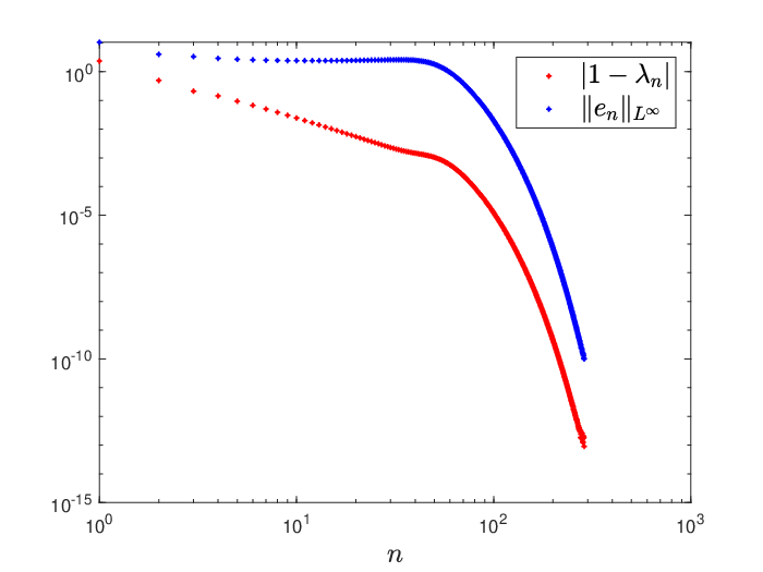
The following proposition justifies these numerical results analytically.

Proposition 5.

The iterative method (34)–(35) diverges from the solitary wave solution $u_{C}$ for any fixed $C\in\mathbb{R}$ .

Proof.

We substitute $w_{n}=u+v_{n}\in H^{1}(\mathbb{R})$ and linearize the iterative method (34)–(35) with respect to $v_{n}$ . For the normalization constant (35), we obtain

\lambda(u+v)=1+\frac{2}{3\int_{\mathbb{R}}u^{2}(u^{\prime})^{2}dx}\int_{\mathbb{R}}(uv+u^{\prime}v_{x}-3u(u^{\prime})^{2}v-3u^{2}u^{\prime}v_{x})dx+\mathcal{O}(\|v\|_{H^{1}}^{2}).

(38)

Writing $\lambda(u+v)=1+\mu(v)+\mathcal{O}(\|v\|_{H^{1}}^{2})$ and substituting it to (34) yields the linearized iterative method:

v_{n+1}=\frac{3}{2}\mu(v_{n})u+\mathcal{M}v_{n},

(39)

where

\mu(v):=\frac{2}{3\int_{\mathbb{R}}u^{2}(u^{\prime})^{2}dx}\int_{\mathbb{R}}(uv+u^{\prime}v_{x}-3u(u^{\prime})^{2}v-3u^{2}u^{\prime}v_{x})dx

(40)

and

\mathcal{M}:=-(1-\partial_{x}^{2})^{-1}(2uu^{\prime\prime}+u^{2}\partial_{x}^{2})

(41)

is the linearized operator. Since $\mathcal{M}u=3u$ , $\mathcal{M}$ is not a contraction in $H^{1}(\mathbb{R})$ ; however it may become a contraction after a constraint imposed by $\lambda$ . In order to add the constraint, we introduce the decomposition $v_{n}=\alpha_{n}u+\xi_{n}$ , where $\alpha_{n}$ is uniquely defined under the orthogonality condition

\int_{\mathbb{R}}(u\xi_{n}+u^{\prime}\partial_{x}\xi_{n}-3u(u^{\prime})^{2}\xi_{n}-3u^{2}u^{\prime}\partial_{x}\xi_{n})dx=0,

(42)

which yields $\mu(\alpha_{n}u+\xi_{n})=-2\alpha_{n}$ . Hence, $\alpha_{n+1}=0$ and $\xi_{n+1}=\mathcal{M}\xi_{n}$ .

The linearized operator (39) is a contraction in $H^{1}(\mathbb{R})$ if the spectrum of $\mathcal{M}$ in $H^{1}(\mathbb{R})$ belongs to the unit disk except for the simple eigenvalue $3$ , for which the eigenvector $u$ is removed by the orthogonality condition (42). By Proposition 6 below, the continuous spectrum of $\mathcal{M}$ is given by ${\rm image}(u^{2})$ . Since ${\rm image}(u^{2})=[0,1+e^{2C}]$ for the solitary wave solution $u_{C}$ with $1+e^{2C}>1$ , $\mathcal{M}$ is not contractive for any fixed $C\in\mathbb{R}$ . Hence, the iterative method (34)–(35) diverges from $u_{C}$ due to the continuous spectrum of $\mathcal{M}$ . ∎

Proposition 6.

Let $u$ be the solitary wave solution $u_{C}$ . The continuous spectrum of the linear operator $\mathcal{M}$ in $H^{1}(\mathbb{R})$ is given by ${\rm image}(u^{2})=[0,1+e^{2C}]$ .

Proof.

Let us consider the spectral problem

\mathcal{M}v=\mu v,\quad v\in H^{1}(\mathbb{R}).

(43)

For simplicity, we work with the cusped soliton $u_{\rm cusp}$ , for which the singularity is placed at one point, $x=0$ . By Theorem 4 in [21, p. 1438], the continuous spectrum of $\mathcal{M}$ is given by the union of the continuous spectra of $\mathcal{M}_{+}$ and $\mathcal{M}_{-}$ restricted on $\mathbb{R}_{\pm}$ subject to the Dirichlet condition at $x=0$ :

\mathcal{M}_{\pm}:=(1-\partial_{x}^{2})^{-1}\left[-u^{2}\partial_{x}^{2}-\frac{2u^{2}}{1-u^{2}}\right]:H^{1}_{0}(\mathbb{R}_{\pm})\mapsto H^{1}_{0}(\mathbb{R}_{\pm}),

(44)

where $H^{1}_{0}(\mathbb{R}_{\pm})$ denote the Sobolev space of $H^{1}(\mathbb{R}_{\pm})$ functions vanishing at $x=0$ . By the symmetry of $u$ , the spectrum of $\mathcal{M}_{+}$ is identical to the spectrum of $\mathcal{M}_{-}$ . Hence, we consider the spectral problem for the operator $\mathcal{M}_{+}$ only.

The Green’s function $G(x,y)$ for $(1-\partial^{2}_{x})G(x,y)=\delta(y)$ in $H^{1}_{0}(\mathbb{R}_{+})$ is given by

G(x,y)=\sinh(x)e^{-y}U(y-x),\quad x,y\in\mathbb{R}_{+},

(45)

where $U$ is the unit step function. Using elementary operations, we can rewrite the spectral problem $\mathcal{M}_{+}v=\lambda v$ for $v\in H^{1}_{0}(\mathbb{R}_{+})$ in the following integral form:

v(x)=\int_{x}^{\infty}G(x,y)\frac{u(y)^{2}[3-u(y)^{2}]}{[u(y)^{2}-\lambda][1-u(y)^{2}]}v(y)dy,\quad x\in\mathbb{R}_{+}.

(46)

The proof that $\sigma_{c}(\mathcal{M}_{+})={\rm image}(u^{2})=[0,1]$ is standard. Indeed, if $\lambda\in{\rm image}(u^{2})$ , then the integral in the right-hand-side of (46) diverges unless $v(x_{\lambda})=0$ at $x_{\lambda}$ given by $u^{2}(x_{\lambda})=\lambda$ , hence the resolvent operator $(\mathcal{M}_{+}-\lambda I)^{-1}$ is unbounded in $H^{1}_{0}(\mathbb{R}_{+})$ . Thus, $\sigma_{c}(\mathcal{M})=\sigma_{c}(\mathcal{M}_{+})\cup\sigma_{c}(\mathcal{M}_{-})={\rm image}(u^{2})=[0,1]$ .

For the case of the solitary wave solution $u_{C}$ with fixed $C\in\mathbb{R}$ , the singularities are placed at two points $x=\pm\ell_{C}$ . Partitioning $\mathbb{R}$ into $(-\infty,-\ell_{C}]\cup[-\ell_{C},\ell_{C}]\cup[\ell_{C},\infty)$ subject to the Dirichlet boundary conditions at $x=\pm\ell_{C}$ gives the same result $\sigma_{c}(\mathcal{M})={\rm image}(u^{2})=[0,1+e^{2C}]$ but the Green’s functions in (46) are expressed differently from the form (45). ∎

Remark 6.

Since ${\rm image}(u^{2})=[0,1]$ for the cusped soliton $u_{\rm cusp}$ , $\mathcal{M}$ is not a strict contraction for the cusped soliton $u_{\rm cusp}$ . Our numerical results on Fig. 13 suggest that $\sigma(M)\backslash\{3\}\subset[-1,1]$ in $H^{1}(\mathbb{R})$ , hence $\mathcal{M}$ is a contraction for the cusped soliton $u_{\rm cusp}$ under the orthogonality condition (42). Despite the lack of strict contraction, the iterative method (34)–(35) converges to the cusped soliton due to discretization and truncation, in agreement with the numerical results shown in Fig. 11 and 12.

Fig. 13 shows the numerical approximation of the spectrum of $\mathcal{M}$ in $H^{1}(\mathbb{R})$ at the cusped soliton $u_{\rm cusp}$ (left) and the bell-shaped soliton $u_{\rm bell}$ (right). The numerical approximations are obtained with the Fourier spectral method. The location of the spectrum of $\mathcal{M}$ agrees with Proposition 6 and Remark 6.

Remark 7.

The cusped soliton $u_{\rm cusp}$ represents the lowest energy state in the continuous family of the solitary wave solutions $u_{C}$ . Indeed, it follows from (18) with $\ell_{C}>0$ for every fixed $C\in\mathbb{R}$ that $E(u_{\rm cusp})\leq E(u_{C})$ . Petviashvili’s method is hence useful to approximate numerically the lowest energy state of the NLS equation.

4.3. Bell-shaped and cusped solitons via Newton method

We represent solutions of the second-order equation (13) as the roots of the nonlinear equation $F(u)=0$ , where

\displaystyle F(u):=-(1-u^{2})\partial_{x}^{2}u+u

(47)

If $u$ is a root of $F$ , then performing a linearization of $F(u+v)$ with respect to $v$ leads to the linearized operator

\displaystyle F(u+v)=\mathcal{L}v+\mathcal{O}(\|v\|_{H^{1}}^{2}),\qquad\mathcal{L}:=-(1-u^{2})\partial_{x}^{2}+\frac{1+u^{2}}{1-u^{2}}.

(48)

Roots of the nonlinear equation $F(u)=0$ in $H^{1}(\mathbb{R})$ can be approximated by using the Newton iterations:

\displaystyle u_{n+1}=u_{n}-\mathcal{L}^{-1}F(u_{n}),\quad n\in\mathbb{N},

(49)

starting with any $u_{1}\in H^{1}(\mathbb{R})$ provided that $\mathcal{L}^{-1}:H^{-1}(\mathbb{R})\mapsto H^{1}(\mathbb{R})$ exists. Note the correspondence $\mathcal{M}=1-(1-\partial_{x}^{2})^{-1}\mathcal{L}$ between linearized operators of the two methods.

The following proposition shows that $\mathcal{L}$ is invertible for the cusped soliton $u_{\rm cusp}$ .

Proposition 7.

Let $u$ be the cusped soliton $u_{\rm cusp}$ . Then, $\sigma(\mathcal{L})=[1,\infty)$ in $L^{2}(\mathbb{R})$ .

Proof.

Let us consider the spectral problem

\mathcal{L}v=\lambda v,\quad v\in{\rm Dom}(\mathcal{L})\subset L^{2}(\mathbb{R}).

(50)

Because $(1-u^{2})^{-1}$ is not integrable near $x=0$ due to singular behavior (21), we have $v(0)=0$ if $v\in{\rm Dom}(\mathcal{L})$ . Multiplying (50) by $v$ and integrating by parts under the condition $v(0)=0$ yields

$\displaystyle\lambda\int_{\mathbb{R}}v^{2}dx$	$\displaystyle=$	$\displaystyle-\int_{\mathbb{R}}(1-u^{2})vv^{\prime\prime}dx+\int_{\mathbb{R}}\frac{1+u^{2}}{1-u^{2}}v^{2}dx$
	$\displaystyle=$	$\displaystyle\int_{\mathbb{R}}(1-u^{2})(v^{\prime})^{2}dx+\int_{\mathbb{R}}(uu^{\prime})^{\prime}v^{2}dx+\int_{\mathbb{R}}\frac{1+u^{2}}{1-u^{2}}v^{2}dx$
	$\displaystyle=$	$\displaystyle\int_{\mathbb{R}}(1-u^{2})(v^{\prime})^{2}dx+\int_{\mathbb{R}}\left[\frac{1+2u^{2}}{1-u^{2}}+(u^{\prime})^{2}\right]v^{2}dx.$

Since $u\in[0,1]$ , we have $\lambda\geq 1$ . Since $u(x)\to 0$ as $|x|\to\infty$ exponentially fast, Weyl’s theory implies that $[1,\infty)\subset\sigma_{c}(\mathcal{L})$ . Hence, $\sigma(\mathcal{L})=[1,\infty)$ for the cusped soliton $u_{\rm cusp}$ . ∎

Remark 8.

For the solitary wave solution $u_{C}$ of Proposition 2 with fixed $C\in\mathbb{R}$ , the weight $(1-u^{2})$ is no longer positive. As a result, $\sigma(\mathcal{L})$ is expected to be sign-indefinite, in agreement with the numerical approximation on Fig. 14 (right).

We study invertibility of $\mathcal{L}$ numerically by rewriting the spectral problem $\mathcal{L}v=\lambda v$ as the generalized eigenvalue problem

\displaystyle\mathcal{A}v=\lambda\mathcal{B}v,\qquad\mathcal{A}:=-(1-u^{2})^{2}\partial_{x}^{2}+(1+u^{2}),\quad\mathcal{B}:=(1-u^{2}).

(51)

In the form (51), the singularity of the potential $\frac{(1+u^{2})}{(1-u^{2})}$ in $\mathcal{L}$ is avoided. The generalized eigenvalue problem (51) can be solved numerically even when $\mathcal{B}$ is not invertible.

Numerical approximations of the spectrum of $\mathcal{L}$ at the cusped and bell-shaped solitons are shown in Fig. 14. The spatial derivatives are replaced by the same Fourier differentiation matrices as before. The numerical results suggest that $\sigma(\mathcal{L})=[1,\infty)$ for the cusped soliton $u_{\rm cusp}$ in agreement with Proposition 7 and $\sigma(\mathcal{L})=(-\infty,\lambda_{0}]\cup[1,\infty)$ with $\lambda_{0}<0$ for the bell-shaped soliton $u_{\rm bell}$ . In both cases, $\mathcal{L}$ is invertible and the Newton iterative method (49) can be used unconditionally.

For solutions from the continuous family $u_{C}$ , numerical results indicate that $\sigma(\mathcal{L}_{+})=(-\infty,\lambda_{C}]\cup[1,\infty)$ , where $\lambda_{C}<0$ depends on $C$ . Figure 15 shows the location of $\lambda_{C}$ with varying $C$ . In agreement with Proposition 7, the results suggest that $\lambda_{C}\to-\infty$ as $C\to-\infty$ , so that the spectrum of $\mathcal{L}$ at for the cusped soliton $u_{\rm cusp}$ reduces to just $[1,\infty)$ .

Figures 16 and 17 show the convergence of the Newton method (49) to the cusped and bell-shaped soliton respectively. As discussed earlier, a key advantage of this method is its enabling to converge from suitable (distinct) initial guesses to both the principal solutions of the IDD model. Another advantage of the method is its ability to converge to arbitrary members $u_{C}$ of the continuous family of solutions. At each step of the iteration, we measure convergence using the distance between successive iterates $\|u_{n+1}-u_{n}\|_{L^{\infty}}$ , and also the approximation error $e_{n}=|F(u_{n})|$ . We stop iterations at step $N$ where the tolerance $\|e_{N}\|_{L^{\infty}}<10^{-10}$ is reached.

5. Spectral stability

In order to derive the spectral stability problem, we use the ansatz

\displaystyle\psi(x,t)=e^{it}[u(x)+e^{\lambda t}(v(x)+iw(x))+e^{\bar{\lambda}t}(\bar{v}(x)+i\bar{w}(x))]

(52)

where $u$ is the solitary wave solution, $v+iw$ is a small perturbation with real $v$ and $w$ , $\lambda$ is the spectral parameter, and the bar denotes complex conjugation. Substituting (52) into the NLS equation (1) and linearizing in $v$ and $w$ gives the spectral stability problem

\displaystyle\left[\begin{array}[]{cc}0&\mathcal{L}_{-}\\ -\mathcal{L}_{+}&0\end{array}\right]\left[\begin{array}[]{c}v\\ w\end{array}\right]=\lambda\left[\begin{array}[]{c}v\\ w\end{array}\right],

where

\displaystyle\mathcal{L}_{+}:=-(1-u^{2})\partial_{x}^{2}+\frac{1+u^{2}}{1-u^{2}},\quad\mathcal{L}_{-}:=

\displaystyle-(1-u^{2})\partial_{x}^{2}+1

Note that $\mathcal{L}_{+}\equiv\mathcal{L}$ is the linearized operator in the Newton method. We consider the spectral problem (5) in $L^{2}(\mathbb{R})$ so that the differential operators $\mathcal{L}_{\pm}$ are closed in

\mathcal{L}_{\pm}:{\rm Dom}(\mathcal{L}_{\pm})\subset L^{2}(\mathbb{R})\mapsto L^{2}(\mathbb{R}),

where ${\rm Dom}(\mathcal{L}_{\pm})=\{v\in L^{2}(\mathbb{R}),\quad(1-u^{2})v^{\prime\prime}\in L^{2}(\mathbb{R})\}$ . The following proposition characterizes the zero eigenvalue of the spectral problem (5) for the cusped soliton.

Proposition 8.

Let $u$ be the cusped soliton $u_{\rm cusp}$ . The spectral problem (5) has a double zero eigenvalue $\lambda=0$ in $L^{2}(\mathbb{R})$ .

Proof.

Due to the phase rotation symmetry of the NLS equation (1), we have

\mathcal{L}_{-}u=-(1-u^{2})u^{\prime\prime}+u=0,

(59)

where $u\in H^{1}(\mathbb{R})$ and $(1-u^{2})u^{\prime\prime}\in H^{1}(\mathbb{R})$ . Hence $(v,w)=(0,u)^{T}$ is the eigenvector of the spectral problem (5) for $\lambda=0$ .

Due to the translation symmetry of the NLS equation (1), we also have

\mathcal{L}_{+}u^{\prime}=-(1-u^{2})u^{\prime\prime\prime}+\frac{1+u^{2}}{1-u^{2}}u^{\prime}=0,

(60)

with $u^{\prime}\in L^{2}(\mathbb{R})$ , however, $(1-u^{2})u^{\prime\prime\prime}\notin L^{2}(\mathbb{R})$ due to the singular behavior (21). Therefore, $(v,w)=(u^{\prime},0)$ is not in the domain of the spectral problem (5) and the geometric multiplicity of $\lambda=0$ is one.

It remains to check the Jordan blocks associated with the eigenvector $(v,w)=(0,u)$ . The first generalized eigenvector satisfies the nonhomogeneous equation

\displaystyle\mathcal{L}_{+}v=-u.

(61)

Since the kernel of $\mathcal{L}_{+}$ is trivial in ${\rm Dom}(\mathcal{L}_{+})\subset L^{2}(\mathbb{R})$ , Fredholm’s alternative theorem implies that there exists $v\in{\rm Dom}(\mathcal{L}_{+})\subset L^{2}(\mathbb{R})$ that solves the nonhomogeneous equation (61). For the cusped soliton, the solution can be found in the explicit form:

v=\frac{1}{2}xu^{\prime},

(62)

since $xu^{\prime}\in H^{1}(\mathbb{R})$ and $(1-u^{2})(xu^{\prime})^{\prime\prime}\in L^{2}(\mathbb{R})$ due to the singular behavior (21).

The second generalized eigenvector, if it exists, satisfies the nonhomogeneous equation

\displaystyle\mathcal{L}_{-}w=v,

(63)

where $v$ is the solution to the nonhomogeneous equation (61). However, no solution $w\in{\rm Dom}(\mathcal{L}_{-})\subset L^{2}(\mathbb{R})$ exists by the Fredholm alternative if

\langle\frac{v}{1-u^{2}},u\rangle\neq 0,

(64)

where we have used the fact that $(1-u^{2})^{-1}\mathcal{L}_{-}$ is a symmetric differential operator. Using (62) and integrating by parts, we obtain

\frac{1}{2}\langle\frac{xu^{\prime}}{1-u^{2}},u\rangle=-\frac{1}{4}\int_{\mathbb{R}}\log(1-u^{2})dx\neq 0,

(65)

where the integration by parts is justified since $x\log(1-u^{2})\to 0$ both as $|x|\to 0$ and as $|x|\to\infty$ . Hence, the algebraic multiplicity of $\lambda=0$ is two. ∎

Remark 9.

The proof of Proposition 8 can be extended to the solution $u_{C}$ with $C\in\mathbb{R}$ up to the nonhomogeneous equation (61). However, $(1-u^{2})(xu^{\prime})^{\prime\prime}\notin L^{2}(\mathbb{R})$ due to the singular behavior (26), hence $v$ is not available in the closed form. Consequently, it is not clear how to show that the constraint (64) holds for the solution $u_{C}$ .

Remark 10.

Besides the result of Proposition 8, it is not clear how to analyze the spectral problem (5) and to prove spectral stability of the cusped soliton. Since $u(x)\to 0$ as $|x|\to\infty$ exponentially fast, the continuous spectrum of the problem is located at $\lambda\in i(-\infty,-1]\cup i[1,\infty)$ . However, $\mathcal{L}_{\pm}$ are not symmetric differential operators compared to the spectral stability problems arising in other NLS-type equations. The case of the solution $u_{C}$ is even more difficult since $1-u^{2}$ is no longer sign-definite.

We approximate the spectral stability problem (5) numerically by using the Fourier discretization matrices. Figure 18 shows the location of the spectrum in the discretized and truncated system (5) for the cusped (left) and bell-shaped (right) solitons. The double zero eigenvalue is detached from the continuous spectrum located on $i(-\infty,-1]\cup i[1,\infty)$ (see Remark 10). Both solitons appear to be spectrally stable for perturbations in $L^{2}(\mathbb{R})$ .

6. Conclusion

We have revisited the prototypical model of the NLS equation with IDD. We have illustrated that the solutions of the model depend on the interplay between the constant coefficient dispersion and the intensity-dependent dispersion. We proved that no solitary wave solutions exist when the two dispersion contributions bear the same sign. On the other hand, the competition between the two leads to a continuous family of solitary wave solutions which are singular at the points of vanishing dispersion, where the constant and intensity-dependent dispersion prefactors cancel each other.

We analyzed three numerical methods which can be used to approximate the relevant solitary waves and showed that the Newton method is robust in approximating different solitary waves of the continuous family, while the regularizing method only converges to the bell-shaped soliton and the Petviashvili method only converges to the cusped soliton being the lowest energy state of the family. We illustrated numerically that the bell-shaped and cusped soliton are spectrally stable in the time-dependent NLS equation.

A number of important outstanding questions remain for further development of the mathematical analysis, including the rigorous proof of the spectral and orbital stability of the solitary waves for which our numerical computations suggest that they are stable. There are also numerous extensions of this class of models that are in their infancy. First off, it is especially relevant to consider if a cancellation of the cubic local nonlinear term (as, e.g., is achieved in BECs in the context of the so-called Feshbach resonances [22]) could be engineered to realize the prototypical IDD model studied herein. Also, one can envision generalizations of the IDD model depending on $|\psi|^{2k}$ and consider the nature of the emerging solutions as a function of $k$ (as has been done in the context of the regular NLS equation [4]). In the same spirit one can envision more complex functional forms of the dispersion coefficient, potentially bearing multiple zero-crossings and attempt to classify the ensuing nonlinear waveforms. Moreover, one can consider lattice-based variants, which could potentially be related to waveguides in optics [23] or associated with optical lattices in BEC [24]. Finally, a natural issue to consider would be the extension of such models into isotropic or anisotropic generalization possibilities into higher dimensions and the dynamics of solitary waves that can arise therein.

References

[1] M.J. Ablowitz and H. Segur, Solitons and the Inverse Scattering Transform, SIAM (Philadelphia, 1981).
[2] M.J. Ablowitz and P.A. Clarkson, Solitons, Nonlinear Evolution Equations and Inverse Scattering, Cambridge University Press (Cambridge, 1991).
[3] M.J. Ablowitz, B. Prinari and A.D. Trubatch, Discrete and Continuous Nonlinear Schrödinger Systems, Cambridge University Press (Cambridge, 2004).
[4] C. Sulem and P.L. Sulem, The Nonlinear Schrödinger Equation, Springer-Verlag (New York, 1999).
[5] A. Hasegawa, Solitons in Optical Communications, Clarendon Press (Oxford, NY 1995).
[6] Yu.S. Kivshar and G.P. Agrawal, Optical solitons: from fibers to photonic crystals, Academic Press (San Diego, 2003).
[7] C.J. Pethick and H. Smith, Bose-Einstein condensation in dilute gases, Cambridge University Press (Cambridge, 2002).
[8] L.P. Pitaevskii and S. Stringari, Bose-Einstein Condensation, Oxford University Press (Oxford, 2003).
[9] M. Kono and M. Škorić, Nonlinear Physics of Plasmas, Springer-Verlag (Heidelberg, 2010).
[10] C. Kharif and E. Pelinovsky and A. Slunyaev, Rogue waves in the ocean, Springer-Verlag (Berlin, 2009).
[11] P. G. Kevrekidis, D. J. Frantzeskakis and R. Carretero-González, The Defocusing Nonlinear Schrödinger Equation, SIAM (Philadelphia, 2015).
[12] A.A. Koser, P.K. Sen, P. Sen, Effect of intensity dependent higher-order dispersion on femtosecond pulse propagation in quantum well waveguides J. Mod. Opt. 56 (2009) 1812-1818.
[13] A.D. Greentree, D. Richards, J.A. Vaccaro, A.V. Durant, S.R. de Echaniz, D.M. Segal, J.P. Marangos, Intensity-dependent dispersion under conditions of electromagnetically induced transparency in coherently prepared multistate atoms, Phys. Rev. A 67 (2003), 023818.
[14] C.Y. Lin, J.H. Chang, G. Kurizki, and R.K. Lee, Solitons supported by intensity-dependent dispersion, Optics Letters 45 (2020), 1471–1474.
[15] G.L. Alfimov, A.S. Korobeinikov, C.J. Lustri, and D.E. Pelinovsky, Standing lattice solitons in the discrete NLS equation with saturation, Nonlinearity 32 (2019), 3445–3484.
[16] V.I. Petviashvili, Equation of an extraordinary soliton, Sov. J. Plasma Phys. 2, 257-258 (1976).
[17] M.J. Ablowitz, Z.H. Musslimani, Spectral renormalization method for computingself-localized solutions to nonlinear systems, Opt. Lett. 30, 2140-2142 (2005).
[18] P. Germain, B. Harrop–Griffiths, and J.L. Marzuola, Compactons and their variational properties for degenerate KdV and NLS in dimension 1, Quart. Appl. Math. 78 (2020), 1–32.
[19] D.E. Pelinovsky, A.V. Slunyaev, A.V. Kokorina, and E.N. Pelinovsky, Stability and interaction of compactons in the sublinear KdV equation, Comm. Nonlin. Science Numer. Simul. (2021), in press.
[20] N. Trefethen, Spectral Methods in MatLab (SIAM, Philadelphia, 2000).
[21] N. Dunford and J.T. Schwartz, Linear Operators. Part II: Spectral Theory (John Wiley & Sons, New York, 1963).
[22] C. Chin, R. Grimm, P. Julienne, E. Tiesinga, Feshbach resonances in ultracold gases, Rev. Mod. Phys. 82 (2010) 1225–1286.
[23] F. Lederer, G. I. Stegeman, D. N. Christodoulides, G. Assanto, M. Segev, and Y. Silberberg, Discrete solitons in optics, Phys. Rep. 463 (2008) 1–126.
[24] O. Morsch, M. Oberthaler, Dynamics of Bose-Einstein condensates in optical lattices, Rev. Mod. Phys. 78 (2006) 179–215.

	$\displaystyle\|x\|$	$\displaystyle=\int_{0}^{v}\frac{d\eta}{\sqrt{\|\log(\eta)\|\left(1+\frac{\log(2-\eta)}{\log(\eta)}\right)}}$
		$\displaystyle=\int_{0}^{v}\frac{d\eta}{\sqrt{\|\log(\eta)\|}}\left[1+\mathcal{O}\left(\frac{1}{\|\log(\eta)\|}\right)\right]\quad\mbox{\rm as}\quad v\to 0^{+}.$		(22)

Localization in optical systems with an intensity-dependent dispersion

Abstract.

1. Introduction

1.1. Main results

Definition 1.

Theorem 1.

Remark 1.

1.2. Organization of the paper

2. Solitary wave solutions of the model

2.1. Solitary wave solutions for b=−1b=-1

Proposition 1.

Proof.

Remark 2.

2.2. Solitary wave solutions for b=1b=1

Proposition 2.

Proof.

Remark 3.

3. Singular behavior near the logarithmic singularity

Proposition 3.

Proof.

Remark 4.

4. Numerical methods for solitary wave solutions

4.1. Bell-shaped soliton via regularization

Proposition 4.

Proof.

Remark 5.

4.2. Cusped soliton via Petviashvili’s method

Proposition 5.

Proof.

Proposition 6.

Proof.

Remark 6.

Remark 7.

4.3. Bell-shaped and cusped solitons via Newton method

Proposition 7.

Proof.

Remark 8.

5. Spectral stability

Proposition 8.

Proof.

Remark 9.

Remark 10.

6. Conclusion

References

2.1. Solitary wave solutions for $b=-1$

2.2. Solitary wave solutions for $b=1$