Gravitational instability of solar prominence threads

We first analyse the situation of the thread initially located at the top of a curved magnetic field (see Fig. 1 top panel). This mass is in equilibrium because the gravity force is zero at $s=L/2$ (see Eq. (1)) and the gradient of the background pressure is zero at the tube apex (see Eq. (3) and Eq. (5)). The goal is to obtain an approximation for the pressure derivative in Eq. (3) once the thread has moved from the initial equilibrium position. In our model we apply line-tying conditions, meaning that pressure fluctuations are not lost along the field lines at the base of the corona. There is no energy leakage through the footpoints and mass flows along the magnetic tube injected from the photosphere are not allowed. Therefore we have perfect reflection at these points because of the big difference in density between the photosphere and corona. It is important to remark that this specific boundary condition allows us to have suspended threads at a given height even in the absence of magnetic dips and that the presence of a chromospheric layer (not included in our model) may affect how the pressure is balanced along the tube.

We denote the length of the thread as $l_{\rm t}$ and by a simple geometrical reasoning $l_{\rm t}/2<s<L-l_{\rm t}/2$ because the thread edge cannot connect with the base of the corona. Under equilibrium at $s=L/2$ the length of the external part of tube that contains the thread is $l_{0}=L/2-l_{\rm t}/2$ along each loop leg (see Fig. 1 top panel). We have the simple relation $L=2l_{0}+l_{\rm t}$. Now we assume that the thread has moved to another location along the magnetic field (see Fig. 1 bottom panel). The distance on the left side is $l_{1}$ now (different from $l_{0}$), while the distance on the right side is $l_{2}$. We have that $l_{1}=s-l_{\rm t}/2$, and $l_{2}=L-l_{1}-l_{\rm t}=L-s-l_{\rm t}/2$. Quiescent prominences are typically $100-200\,{\rm Mm}$ long ($L$) and are about a 100-fold denser than the surrounding corona ($\rho_{\rm t}/\rho_{0}$). However, it is known that the entire bodies of prominences consist in a collection of individual short threads of plasma located in long field lines so that only a fraction of each field line ($l_{\rm t}$) is filled with dense plasma. In this study a wide range of thread parameters are utilised to exemplify a vast sort of prominence threads (see Mackay et al. 2010; Engvold 2015, for a detailed description of solar prominences).

Since the system is assumed to be dissipationless, we consider that the evolution during the motion of the thread is adiabatic. The behaviour of the plasma in the evacuated parts of the tube, that is where the density is low, is similar to that of a piston because of the line-tying conditions at the footpoints. The gas pressure can be written as the background, stratified from gravity, plus a term that depends on the position of the thread. The key idea is to apply the adiabatic law to each part of the tube, but to this term only, removing the contribution from the background,

where $p_{0}$ represents the reference pressure before the thread has moved, changing the length of the evacuated part from $l_{0}$ to $l_{1}$ and pressure from $p_{0}$ to $p_{1}$ for the left side. For the right side we have changes from $l_{0}$ to $l_{2}$ and from $p_{0}$ to $p_{2}$. Since we are considering a perfectly circular geometry we have that $A_{0}=A_{1}=A_{2}$ and the cross-sectional areas cancel in the previous expressions. Now from Eq. (3.1) we obtain that

The hydrostatic equation for the thread is therefore

Using Eq. (3) for the sound speed together with the previous expressions for pressure and gravity we obtain the following equation for $s$, representing the location under static equilibrium of the dense thread along the tube,

where $c^{2}_{{\rm s0}}=\gamma p_{0}/\rho_{0}$, and $\rho_{\rm t}/\rho_{0}$ corresponds to the density contrast between the thread and the density background at $s=L/2-l_{\rm t}/2$. The parameter $\rho_{\rm t}/\rho_{0}$ must be much larger than 1 since we are not taking into account any energy flux through the thread and its mass and length are assumed to be constant.

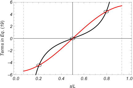
Equation (31) is transcendental and has to be solved numerically. From now on we denote $s_{\rm e}$ a solution of Eq. (31). It is easy to verify that $s_{\rm e}=L/2$ is a solution for any values of the parameters. Hence, there is always an equilibrium solution at the tube apex ($s_{\rm e}^{\mathscr{A}}=L/2$) that can be stable or unstable. Furthermore, the symmetry of the model with respect to $s=L/2$ implies that if there are additional solutions, they appear in pairs ($s_{\rm e}^{\mathscr{L}},s_{\rm e}^{\mathscr{R}}$) verifying $s_{\rm e}^{\mathscr{L}}+s_{\rm e}^{\mathscr{R}}=L$, to wit, the solutions are distributed symmetrically with respect to $s=L/2$: one on the left ($s_{\rm e}^{\mathscr{L}}$) and the other on the right side ($s_{\rm e}^{\mathscr{R}}$) of the tube.

To understand the nature of the these possible situations, in Fig. 2 we plotted the left- and right-hand side terms of Eq. (31) as a function of $s$, for fixed parameters $L$, $c_{{\rm s0}}$, $g$, $\rho_{\rm t}/\rho_{0}$, and varying $l_{\rm t}$ using the projected gravity given in Eq. (1). The gravity acceleration is $g=274\,{\rm m\,s^{-2}}$, and we take a spatial reference length of $H=10,000\,{\rm km}$. The sound speed takes a value of $c_{{\rm s0}}=166\,{\rm km}\,{\rm s^{-1}}$ for a fully ionised coronal tube with $10^{6}$ K temperature. When the two curves cross (see circles) we have a solution at that particular point. On the top panel we have only one solution: the trivial one at $s_{\rm e}^{\mathscr{A}}=L/2$. On the bottom panel however three solutions appear: the trivial one plus two complementary solutions. As we describe in Sect. 4, in the first situation the mass remains at its original position, and, upon being subject to a small disturbance, it oscillates around this point because this equilibrium is stable. In the second situation, the mass is not stable at the initial position at the apex, and after being perturbed the mass moves to one of the solutions along the legs that are energetically more favourable. The stability analysis performed in this and in the following sections provides a simple criterion that tells us when a plasma thread is gravitationally stable or unstable.

We discuss the results from the physical point of view. Figure 2 shows that the existence of the non-trivial solutions of Eq. (31) depends on the thread model parameters. Figure 3 (top panel) shows the equilibrium position $s_{\rm e}$ as a function of $\rho_{\rm t}/\rho_{0}$ for different values of $L$ when the thread length is $l_{\rm t}=0.1\,H$. We obtain that the system only develops the $s_{\rm e}^{\mathscr{L}}$ and the $s_{\rm e}^{\mathscr{R}}$ solutions for values of $\rho_{\rm t}$ beyond ${\rho_{\rm t}}_{\rm b}$. When $\rho_{\rm t}<{\rho_{\rm t}}_{\rm b}$, meaning before the appearance of the bifurcation, $s_{\rm e}^{\mathscr{A}}$ is the only equilibrium position, so that we are in the situation of the top panel of Fig. 2 and therefore $s_{\rm e}^{\mathscr{A}}/L=0.5$ is stable. However, when the thread structure enables the existence of two complementary solutions, these are energetically more suitable so that $s_{\rm e}^{\mathscr{A}}$, which remains located at $s_{\rm e}/L=0.5$ (see horizontal dashed lines in Fig. 3 top panel), becomes an unstable solution. To distinguish between stable or unstable solutions, we represent in Fig. 3 (and in the following figures) stable solutions as solid curves and unstable solutions as dashed curves. In addition, we realise that for the three values of $L$, $s_{\rm e}^{\mathscr{L}}$ and $s_{\rm e}^{\mathscr{R}}$ appear around the same bifurcation value ${\rho_{\rm t}}_{\rm b}$. This means that the bifurcation density value from which we obtain an equilibrium out of the apex of the structure, does not strongly depend on the length of the magnetic tube. We note that $s_{\rm e}$ is normalised to $H$ for normalisation purposes since if we keep the normalisation to $L$, the solutions of the three configurations overlap. This means that the normalised $s_{\rm e}/L$ does not depend strongly on $L$ for this set of parameters. This feature is clearer in the bottom panel of Fig. 3, where $s_{\rm e}$ as a function of $L$ is plotted; when $L$ is large the stable solutions are almost horizontal. Moreover, as was expected, the equilibrium position of the thread drops with increasing $\rho_{\rm t}$. It is interesting to study the dependence of the equilibrium position on the thread length. Figure 3 (middle panel) shows $s_{\rm e}$ as a function of $l_{\rm t}/L$ for different values of $L$ when $\rho_{\rm t}/\rho_{0}=100$. For $L=10\,H$ we obtain that below the bifurcation $s_{\rm e}=s_{\rm e}^{\mathscr{A}}$ is the only solution of Eq. (31) and this is stable, but when $l_{\rm t}>{l_{\rm t}}_{\rm b}$, $s_{\rm e}^{\mathscr{A}}$ becomes unstable and the emerged branches $s_{\rm e}^{\mathscr{L}}$ and $s_{\rm e}^{\mathscr{R}}$ are stable. For $L=15\,H$ and $L=20\,H$ the bifurcation thread length is out of the plot and their $s_{\rm e}^{\mathscr{A}}$ overlaps with that for $L=10\,H$ at $s_{\rm e}/L=0.5$. In Fig. 3 (middle panel) we also see that the equilibrium position of the thread changes along the magnetic tube when the thread length increases. Figure 3 (top and middle panels) show the same behaviour for all sets of parameters, which consists in a sole stable solution for values below the bifurcation, and two symmetric stable solutions out of the apex plus an unstable solution at $s_{\rm e}=L/2$ beyond the bifurcation point. However, Fig. 3 (bottom panel) shows that for some set of parameters, the system does not present the $s_{\rm e}^{\mathscr{L}}$ and $s_{\rm e}^{\mathscr{R}}$ equilibria when $L$ varies so that $s_{\rm e}^{\mathscr{A}}$ is always stable. Interestingly, the bottom panel of Fig. 3 shows that for small changes of $\rho_{\rm t}$, $s_{\rm e}^{\mathscr{L}}$ and $s_{\rm e}^{\mathscr{R}}$ vary significantly. Moreover, we see that the bifurcation length $L_{\rm b}$ for $\rho_{\rm t}/\rho_{0}=133$ and $\rho_{\rm t}/\rho_{0}=138$ is short, around $L_{\rm b}=2.7\,H$ and $L_{\rm b}=1.4\,H$, respectively. These values are shorter than the typical magnetic tube observations.

More aspects about the bifurcation values and how to calculate them are given in Sect. 4. But we finish this section by analysing the presented results from a dynamical systems perspective. The transition from one stable equilibrium solution to two symmetric stable solutions and one unstable solution is characteristic of the supercritical pitchfork bifurcation (see e.g. Sect. 3.4 of Strogatz 2018 or Sect. 20.1E of Wiggins 2003). This bifurcation is present in systems that have a symmetry, such as the symmetry between the left and right sides of our magnetic tube when the thread is initially at the tube apex. In Fig. 3 we find the same type of pitchfork bifurcation in the three panels, although in the bottom panel the unstable solutions for $\rho_{\rm t}/\rho_{0}=133$ and $\rho_{\rm t}/\rho_{0}=138$ are overplotted by the stable solution of $\rho_{\rm t}/\rho_{0}=129$.

It is straightforward to derive analytical expressions for the situation of a thread initially located at any position along the tube, denoted by $s_{0}$, and not necessarily at $L/2$ as discussed in the previous section. We simply need to rewrite Eq. (3.1) as

and the corresponding equilibrium equation analogous to Eq. (31) becomes

Equation (35) simplifies to Eq. (31) when $s_{0}=L/2$. Different types of representative solutions are shown in Fig. 4 and in this case the parameter that has been chosen to change is $\rho_{\rm t}$ (in Fig. 2 it was $l_{\rm t}$). In these plots the initial position of the thread is $s_{0}=0.4/L$, therefore located on the left half of the tube. The left-hand side of Eq. (35) is not symmetric anymore with respect to the tube apex, and this facilitates the existence either of one, two, or three solutions, according to Fig. 4. But we note that by continuity there must be a situation in these circumstances with two solutions when the left- and right-hand curves are tangential. This case is calculated as in Sect. 3.1 by imposing that the spatial derivatives of the left- and right-hand sides of Eq. (35) are equal as follows:

Thus, Eq. (36) has to be satisfied together with Eq. (35) for the system to have two equilibrium solutions. An example of such a situation is found in Fig. 4 middle panel. For simplicity, we still denote the equilibrium position on the left side of the tube as $s_{\rm e}^{\mathscr{L}}$, as $s_{\rm e}^{\mathscr{R}}$ on the right side, and as $s_{\rm e}^{\mathscr{A}}$ for the central near apex solution, so that when the system has only two equilibrium solutions, $s_{\rm e}^{\mathscr{R}}=s_{\rm e}^{\mathscr{A}}$ (or $s_{\rm e}^{\mathscr{L}}=s_{\rm e}^{\mathscr{A}}$). As in Sect. 3.1 the sign of the difference between the left-hand term and the right-hand term of Eq. (36) reveals the nature of the different solutions.

In the bifurcation diagram we find that the characteristic pitchfork for the symmetric case disconnects into two curves: one below $s_{0}/L=0.5$ and another above this value. An example is shown in Fig. 5 (top panel) when the density contrast is changed. The lower curve is always stable, whereas the upper curve has both stable and unstable branches. Therefore, the pitchfork bifurcation occurring in the symmetrical case is essentially replaced in the non-symmetrical case by a stable state (lower curve) alongside a saddle-node bifurcation (upper curve). As we increase the density contrast there is no longer a sharp transition at the bifurcation point representative of the symmetric case (compare with Fig. 3). Hence, the equilibrium position of the thread varies smoothly with the density contrast on the lower stable curve. Furthermore, the stable branch of the upper curve, which is also a permitted equilibrium state of the system, is not accessible unless the thread is given a large initial disturbance, thereby making this equilibrium more favourable. Qualitatively similar results are obtained for the bifurcation diagrams as a function of the thread length and the total length in the middle and bottom panels of Fig. 5, respectively. As was expected, when $s_{0}/L\rightarrow 0.5$, the diagrams approach those in Fig. 3, characterised by a stable solution at $s_{\rm e}/L=0.5$ below the bifurcation values; however we see that the two curves (upper and lower) still remain disconnected for $s_{0}/L=0.49$.

Figure 6 shows the situation when there is a transition between one to three solutions (orange lines, $\rho_{\rm t}/\rho_{0}=200$) when the initial position of the thread, $s_{0}$, is changed. One of the emerging solutions around $s_{0}/L=0.3$, $s_{\rm e}^{\mathscr{A}}$, is unstable, while the other solution, $s_{\rm e}^{\mathscr{R}}$, is stable. This behaviour is similar to that found for the symmetric case with $s_{0}=L/2$ described earlier. In Fig. 6 a case with no bifurcations but with multiple solutions for fixed parameter values ($\rho_{\rm t}/\rho_{0}=400$) is also represented. The solutions that are around the apex (dashed curves) have a different behaviour with respect to the left- and right-hand solutions. In this case $s_{\rm e}^{\mathscr{A}}$ decreases when $s_{0}$ is raised, while for the other two solutions $s_{\rm e}^{\mathscr{L}}$ and $s_{\rm e}^{\mathscr{R}}$ increase with $s_{0}$. When $s_{0}$ moves closer to the tube apex, $s_{\rm e}^{\mathscr{A}}\rightarrow L/2$ and this solution is unstable. In conclusion, given that the initial thread position, $s_{0}$, is not at the apex, this parameter breaks the symmetry of the system. In bifurcation theory it is called an imperfection parameter. The resulting bifurcation diagram of Fig. 6 is no longer symmetric about a horizontal line and possesses an S-shape (see Wang 1994 and Sect. 3.6 of Strogatz 2018). The orange curve in this figure has a lower and an upper bifurcation point, $s_{0,{\rm l}}/L\simeq 0.3$ and $s_{0,{\rm u}}/L\simeq 0.7$, respectively. This S-shaped bifurcation curve can be thought of as the composition of two saddle-node bifurcation curves, the lower (upper) one with its bifurcation point at $s_{0}=s_{0,{\rm l}}$ ($s_{0}=s_{0,{\rm u}}$). The black curve of Fig. 6 is a special case of an S-shaped bifurcation curve because the lower and upper bifurcation points are outside the range of validity of the parameter $s_{0}$. Therefore, the system always supports three solutions.

We start with the trivial solution at the tube apex. We consider a small longitudinal displacement, $\delta s$, of the centre of the plasma thread. We assume that $\delta s\ll L$ because we are interested in the linear regime. The restoring forces acting on the plasma thread are the pressure gradient and the projected gravity force. Let us write the pressure at both sides of the thread as a function of the displacement with respect to $L/2$, the equilibrium position. Using the adiabatic assumption again, the pressure on the left and right parts of the tube is given by

The terms in parenthesis are written as

where in the last step we used the Maclaurin series approximation for small arguments (because $\delta s/L\ll 1$). This approximation is crucial to find the linear result we are looking for, since pressure fluctuations are now linearly proportional to $\delta s$. We have that

and the pressure gradient is given by

For the projected gravity around $s=L/2$ it is not difficult to see that Eq. (1) reduces to a sinus of $\delta s$,

where we again used the approximation for small arguments in the last step.

We have expressions for all the terms that appear in the momentum equation, that is Eq. (6) for $s=L/2+\delta s$, which is now

The right-hand side term of this equation is proportional to $\delta s$ only. The solution to the differential equation is of the form $e^{i\omega t}$ and we have that

where the sound speed of the background was used. According to Eq. (43) we realise that we can have the following situations: $\omega^{2}>0$ ($\omega$ real), meaning that the motion is purely oscillatory around a stable equilibrium; $\omega^{2}<0$ ($\omega$ purely imaginary), indicating that the system is unstable; and $\omega^{2}=0$. This is the expected situation based on the results of Sect. 3 about the equilibrium. Interestingly, it is not difficult to see that the growth rates and frequencies derived from the dispersion relation in Eq. (43) are exactly the same $\tau$ and $\omega$ found in Sect. 3.1 and derived from a mathematical point of view.

The transition between the two regimes ($\omega^{2}=0$) provides helpful information because it corresponds to a bifurcation point, where, as we have seen, the number of solutions and/or their stability can change. This transition takes place when the following condition for the density contrast is satisfied:

where the density contrasts below this bifurcation value correspond to a stable solution, whereas for $\rho_{\rm t}>{\rho_{\rm t}}_{\rm b}$ the stable solution turns unstable. This behaviour is shown in Fig. 7 (top panel), in which $\omega^{2}$ is plotted as a function of $\rho_{\rm t}/\rho_{0}$ for different values of $L$ and for the three possible equilibrium positions $s_{\rm e}^{\mathscr{A}}$, $s_{\rm e}^{\mathscr{L}}$, and $s_{\rm e}^{\mathscr{R}}$. Since the initial position of the thread is at the apex of the structure, $s_{\rm e}^{\mathscr{L}}$ and $s_{\rm e}^{\mathscr{R}}$ are symmetric and have the same frequency, so only one solid curve with $\omega^{2}>0$ is visible to the right of the bifurcation point. Frequencies associated with $s_{\rm e}^{\mathscr{A}}$ are found at the right of the bifurcation point and below zero in Fig. 7. We see that the bifurcation density, which delimits stable solutions (solid curves) with unstable (dashed curves), does not strongly depend on $L$. This behaviour agrees with Eq. (44), which simplifies to ${\rho_{\rm t}}_{\rm b}/\rho_{0}=\frac{4\,c^{2}_{{\rm s0}}\,}{g\pi\,l_{\rm t}}$ when $l_{\rm t}$ is neglected with respect to $L$.

Assuming that $\rho_{\rm t}/\rho_{0}$ and $L$ are fixed, then we have a bifurcation length for the thread that determines if the solution is stable or unstable as follows:

(see middle panel of Fig. 7). For typical prominence values the term inside the square root is always positive and the square root of this term is smaller than 1, providing a physically acceptable value (${l_{\rm t}}_{\rm b}>0$). The equilibrium positions of threads with lengths shorter than ${l_{\rm t}}_{\rm b}$ are always stable.

Finally, from Eq. (43) we find that the bifurcation length of the magnetic field lines is given by

and the term in the denominator is not necessarily positive. A negative bifurcation length is non-physical, meaning that in this situation it is not possible to find a transition from the stable to the unstable regime. Therefore, when

the bifurcation length is negative, thereby implying in our case that the solution is always stable ($\omega^{2}>0$) independent of the length $L$; this is easy to check introducing the condition given by Eq. (47) into Eq. (43). Figure 7 (bottom panel) shows $\omega^{2}$ as a function of $L$ for different values of $\rho_{\rm t}$ and we find a case in which Eq. (47) is satisfied and $\omega^{2}$ is always positive. For values of the parameters that make the left-hand side of Eq. (47) less than 1, the solution is either stable or unstable, depending on the length of the field lines, if $L<L_{\rm b}$ the system that only develops $s_{\rm e}^{\mathscr{A}}$ is stable and if $L>L_{\rm b}$ it is unstable (see lower branch curves in bottom panel of Fig. 7). Interestingly, the bifurcation length $L_{\rm b}$ depends strongly on the density contrast (see the short range of $\rho_{\rm t}/\rho_{0}$ in Fig. 7 bottom panel). We note that to have a stable solution the three criteria must be simultaneously satisfied; these criteria are $\rho_{\rm t}<{\rho_{\rm t}}_{\rm b}$, $l_{\rm t}<{l_{\rm t}}_{\rm b}$, and $L<L_{\rm b}$ or equivalently Eq. (47) for the length of the field lines. This is an interesting result that provides useful information about the behaviour of the system depending on the parameters.

It is worthy noting that the first term on the right-hand side of Eq. (43) is the frequency squared of a slow mode in a slab model of length $l_{\rm t}$ inside a field line with a length of $L$ (Joarder & Roberts 1992; Díaz et al. 2010; Soler et al. 2010). Luna et al. 2012 derived a similar expression for the frequency but for a magnetic field with a dip at the location of the thread. In their formula the sign in front of the gravitational term is positive and therefore the instability is not present in their configuration; their system is always (linearly) stable because they consider a concave upwards geometry for the magnetic field.

Now we generalise the frequency of oscillation for any equilibrium position, $s_{\rm e}$, along the tube and hence we do not restrict the analysis to the equilibrium solution at the tube apex. But we note that the thread is still initially located at $s=L/2$. Under these conditions we have that

where $p_{10}$ and $p_{20}$ correspond to the equilibrium pressures that satisfy Eq. (3.1). We rewrite ${p_{1}}$ as

where we used the Maclaurin series approximation for small arguments, but if $s_{\rm e}$ is similar to $l_{\rm t}/2$ the approximation is not valid. An analogous expression is derived for ${p_{2}}$. The pressure gradient using the previous equations is approximated by

For the projected gravity we need to perform a Taylor expansion of the cosine around the equilibrium position, which is now $s_{\rm e}$,

where we only retain up to linear terms in $s-s_{\rm e}$. We have that $\delta s=s-s_{\rm e}$ according to our notation.

Finally, using the same procedure as before we derive an expression for the oscillation frequency of a thread around the final equilibrium position $s_{\rm e}$, which has been achieved from an initial location of the thread at $s_{0}\neq L/2$. The corresponding pressures at the edge of the thread due to a small displacement $\delta s$ from the equilibrium position are expressed as Eq. (4.1), but now $p_{10}$ and $p_{20}$ correspond to the equilibrium pressures that satisfy Eq. (3.2). Using similar approximations to those in Eq. (49) and cancelling the equilibrium terms according to Eq. (35), we eventually find that the frequency squared is written as

The previous frequency expressions given in Eq. (43) when $s_{0}=s_{\rm e}=L/2$ and Eq. (52) when $s_{0}=L/2$, $s_{\rm e}\neq L/2$ are recovered in Eq. (53). In this equation $s_{\rm e}$ must be a solution to Eq. (35). Obtaining analytical bifurcation values, except for the trivial case ($s_{0}=s_{\rm e}=L/2$), is much more difficult now and it is only possible for the bifurcation density contrast. The rest of bifurcation values are determined numerically. As expected from bifurcation theory, imposing the condition for a bifurcation value, that is $\omega^{2}=0$ in Eq. (53), is completely equivalent to the condition given by Eq. (36) that determines the bifurcation point based only on the equilibrium configuration. This is confirmed by the comparison of the bifurcation values in Fig. 8 and the respective results in Fig. 5. This is also a solid indication that the performed eigenfrequency analysis in this section is coherent.

Now the break of symmetry due to the imperfection parameter $s_{0}$ causes the difference between the frequency squared of $s_{\rm e}^{\mathscr{L}}$ and $s_{\rm e}^{\mathscr{R}}$. This is visible in the plotted upper curves of Fig. 8 (solid curves). Beyond the bifurcation values two branches appear that correspond to $s_{\rm e}^{\mathscr{R}}$ and $s_{\rm e}^{\mathscr{A}}$, which are positive for $s_{\rm e}^{\mathscr{R}}$ (solid curves) and negative for $s_{\rm e}^{\mathscr{A}}$ (dashed curves). Logically, when $s_{0}/L\rightarrow 0.5$ (purple curves), $\omega^{2}$ for $s_{\rm e}^{\mathscr{R}}$ approaches the same value as for $s_{\rm e}^{\mathscr{L}}$. For $s_{\rm e}^{\mathscr{R}}$ (emerging at the bifurcation point), $\omega^{2}$ increases with $\rho_{\rm t}/\rho_{0}$ (top panel) and $l_{\rm t}/H$ (middle panel). For $s_{\rm e}^{\mathscr{L}}$, stable in the whole parameter range, $\omega^{2}$ decreases with $\rho_{\rm t}/\rho_{0}$ and $l_{\rm t}/H$ until it reaches a minimum located before the bifurcation point from where it starts increasing. On the contrary, in the bottom panel of Fig. 8 we see that for $s_{\rm e}^{\mathscr{L}}$ the frequency decreases for large values of $L$.

In Fig. 9 the three square of the frequencies corresponding to the solutions in Fig. 6 are plotted as a function of the initial position of the thread, $s_{0}$. To calculate these frequencies, we used the values of $s_{\rm e}$ that satisfy Eq. (35). We note that $s_{\rm e}^{\mathscr{L}}$ and $s_{\rm e}^{\mathscr{R}}$ are always stable while $s_{\rm e}^{\mathscr{A}}$ is always unstable. As expected from physical grounds the left and right side solutions converge to the same value when there is symmetry in the system, that is for $s_{0}=L/2$; we note that beyond this point the meaning of $s_{\rm e}^{\mathscr{L}}$ and $s_{\rm e}^{\mathscr{R}}$ has to be inverted. We also observe the transition between one and three solutions for a specific choice of parameters ($\rho_{\rm t}/\rho_{0}=200$, orange curves). At the bifurcation point two solutions emerge from $\omega=0$: one representing a stable solution ($s_{\rm e}^{\mathscr{R}}$) and another corresponding to an unstable solution ($s_{\rm e}^{\mathscr{A}}$). We also see that $\omega^{2}$ significantly varies with $s_{0}/L$ for stable solutions, but it is essentially independent of $s_{0}/L$ for unstable solutions.