Error estimate of the Non Intrusive Reduced Basis method with finite volume schemes

Abstract

The context of this paper is the simulation of parameter-dependent partial differential equations (PDEs). When the aim is to solve such PDEs for a large number of parameter values, Reduced Basis Methods (RBM) are often used to reduce computational costs of a classical high fidelity code based on Finite Element Method (FEM), Finite Volume (FVM) or Spectral methods. The efficient implementation of most of these RBM requires to modify this high fidelity code, which cannot be done, for example in an industrial context if the high fidelity code is only accessible as a ”black-box” solver. The Non Intrusive Reduced Basis method (NIRB) has been introduced in the context of finite elements as a good alternative to reduce the implementation costs of these parameter-dependent problems. The method is efficient in other contexts than the FEM one, like with finite volume schemes, which are more often used in an industrial environment. In this case, some adaptations need to be done as the degrees of freedom in FV methods have different meanings. At this time, error estimates have only been studied with FEM solvers. In this paper, we present a generalisation of the NIRB method to Finite Volume schemes and we show that estimates established for FEM solvers also hold in the FVM setting. We first prove our results for the hybrid-Mimetic Finite Difference method (hMFD), which is part the Hybrid Mixed Mimetic methods (HMM) family. Then, we explain how these results apply more generally to other FV schemes. Some of them are specified, such as the Two Point Flux Approximation (TPFA).

Elise Grosjean ¹¹ 1 Sorbonne Université and Université de Paris, CNRS, Laboratoire Jacques-Louis Lions (LJLL), F-75005 Paris, France, Yvon Maday ¹¹ 1 Sorbonne Université and Université de Paris, CNRS, Laboratoire Jacques-Louis Lions (LJLL), F-75005 Paris, France ²² 2 Institut Universitaire de France

Keywords: Reduced Basis Method, Finite Volume Method

Introduction

This paper is concerned with the efficient simulation of parameter-dependent partial differential equations (PDEs), with a parameter varying in a given set $\mathcal{G}$ . For complex physical systems, computational costs can be huge. It may happen, for instance in the context of parameter optimization or real time simulations in an industrial context, that the same problem needs to be solved for several parameter values.

In such cases, different model order reductions (MOR) like the reduced basis methods have been proposed (see eg [25, 21]) based on POD or greedy selection of the reduced basis, the reduced basis elements being computed accurately enough through a high fidelity code. In these approaches, the efficient implementation of the reduced method, leading to reductions in the computational time, requires to be able to deeply enter into the high fidelity code, in order to compute offline, a key ingredient which saves the implementation costs online. This can be tedious, even impossible when the code has been bought, as it is often the case in an industrial context. The Non Intrusive Reduced Basis methods (NIRB) [24, 7] has been proposed in this framework. This method is useful to reduce computational costs of parametric-dependent PDEs in a non intrusive way. Unlike other MOR, the NIRB method does not require to modify the solver code and hence does not depend on the numerical approach underlying the code. This method, based on two grids, one fine where high fidelity computations are done offline and one coarse which is used online, has been introduced in [24, 7]. It was presented and analysed in the case where the high fidelity code is based on a finite element solver. In these papers, an optimal error estimate is recovered and illustrated with numerical simulations. The method can be extended to other classical discretizations but the key ingredient is a better approximation rate in the $L^{2}$ norm than in the energy norm, thanks to the Aubin-Nitsche’s trick that is easy for variational approximations. In addition, the degrees of freedom in FVM don’t have the same status as in FEM and the transfer of information from one grid to another must be adapted. The aim of this paper is to propose the adaptation of the NIRB method to FV and to propose the numerical analysis able to recover the classical error estimate with Finite Volume (FV) schemes.

The Non Intrusive Reduced Basis Method.

Let $\Omega$ be an open bounded domain in $\mathbb{R}^{d}$ with $d\leq 3$ . The NIRB method in the context of a high fidelity solver of finite element or finite volume types involves two partitioned meshes, one fine mesh $\mathcal{M}_{h}$ and one coarse mesh $\mathcal{M}_{H}$ , where $h$ and $H$ are the respective sizes of the meshes and $h<\!<H$ . The size $h$ (res. $H$ ) is defined as $h=\underset{K\in\mathcal{M}_{h}}{\max\ }h_{K}$ (resp. $H=\underset{K\in\mathcal{M}_{H}}{\max\ }H_{K}$ ) where the diameter $h_{K}$ (or $H_{K}$ ) of any element $K$ in a mesh is equal to $\underset{x,y\in K}{\sup\ }|x-y|$ .

As it is classical in other reduced basis methods, the NIRB method is based on the assumption (assumed or actually checked) that the manifold of all solutions $\mathcal{S}=\{u(\mu),\mu\in\mathcal{G}\}$ has a small Kolmogorov n-width $\varepsilon(n)$ [23]. This leads to the fact that very few well chosen solutions are sufficient to approximate well any element in $\mathcal{S}$ . These well chosen elements are called the snapshots. In this frame, the method is based on two steps : one offline step and one online. The “offline” part is costly in time because the snapshots must be generated with a high fidelity code on the fine mesh $\mathcal{M}_{h}$ . The “online” step is performed on the coarse mesh $\mathcal{M}_{H}$ , and thus much less expensive than a high fidelity computation. This algorithm remains effective as the offline part is performed only once and in advance and also independently from the online stage. The online stage can then be done as many times as desired.

•

In the offline part, several snapshots are computed on the fine mesh for different well chosen parameters in the parameter set $\mathcal{G}$ with the (fine and costly) solver. The best way to determine the required parameters is through a greedy procedure [29, 1, 5] if available or through an SVD approach.
•

The online part consists in computing a coarse solution with the same solver for some (new) parameter $\mu\in\mathcal{G}$ and then $L^{2}$ -project this (coarse) solution on the (fine) reduced basis. This results in an improved approximation, in the sense that we may retrieve almost fine error estimates with a much lower computational cost.

Motivation and earlier works.

Several papers have underlined the efficiency of the NIRB method in the finite element context, illustrated both with numerical results presenting error plots and the online part compurational time [24, 7, 9, 8]. However, to the best of our knowledge, works with Finite Volume (FV) schemes have not yet been studied with a non intrusive approach [22, 28, 20, 27, 6], and they are often preferred to finite element methods in an industrial context. Thanks to recent works on super-convergence [18], and with some technical subtleties, we are now able to generalize the two-grids method which is non intrusive to FV methods and propose the numerical analysis of this method.

Main results.

In the context of $P_{1}$ -FEM solvers, the works [24, 7] retrieve an estimate error of the order of $\mathcal{O}(h+H^{2})$ in the energy norm using the Aubin-Nitsche’s Lemma [3] for the coarse grids solution (for a reduced basis dimension large enough). With FV schemes, no equivalent of the Aubin-Nitsche’s lemma is available, instead, we consider the class of Hybrid Mimetic Mixed methods (HMM) schemes for elliptic equations and use a super-convergence property proven in ( [12, 18, 13]).
Let us consider the following linear second-order parameter dependent problem as our model problem:

		$\displaystyle-\ \textrm{div}(A(\mu)\nabla u)=f\textrm{ in }\Omega,$			(1a)
		$\displaystyle u=0\textrm{ on }\partial\Omega,$			(1b)

where $f\in L^{2}(\Omega)$ , $\mu$ is a parameter in a set $\mathcal{G}$ , and for any $\mu\in\mathcal{G}$ , $A(.;\mu)\mathrel{\mathop{\mathchar 58\relax}}\Omega\to\mathbb{R}^{d\times d}$ is measurable, bounded, uniformly elliptic, and $A(\textbf{x};\mu)$ is symmetric for a.e. $\textbf{x}\in\Omega$ .

Under general hypotheses, it is well known that this problem has a unique solution.

The usual weak formulation for problem (1a)-(1b) reads:
Find $u\in H_{0}^{1}(\Omega)$ such that,

\forall v\in H_{0}^{1}(\Omega),\quad a(u,v;\mu)=(f,v),

(2)

where

a(w,v;\mu)=\int_{\Omega}A(\textbf{x};\mu)\nabla w(\textbf{x})\cdot\nabla v(\textbf{x})\ d\textbf{x},\quad\forall w,v\in H_{0}^{1}(\Omega).

The main result of this paper is the following estimate:

Theorem 0.1 (NIRB error estimate for hMFD solvers).

Let $u_{hH}^{N}(\mu)$ be the reduced solution projected on the fine mesh and generated with the hMFD solver with the unknowns defined on $\textbf{x}_{k}=\overline{\textbf{x}}_{K}$ (the cell centers of mass), and $u(\mu)$ be the exact solution of (2) under an $H^{2}$ regularity assumption (8) (which will be stated later), then the following estimate holds

\mathinner{\!\left\lVert u(\mu)-u_{hH}^{N}(\mu)\right\rVert}_{\mathcal{D}}\leq\varepsilon(N)+C_{1}h+C_{2}(N)H^{2},

(3)

where $C_{1}$ and $C_{2}$ are constants independent of $h$ and $H$ , $C_{2}$ depends on $N$ , the number of functions in the basis, and $\mathinner{\!\left\lVert\cdot\right\rVert}_{\mathcal{D}}$ is the discrete norm introduced in section 1, and $\varepsilon$ depends of the Kolmogorov n-width. If $H$ is such as $H^{2}\sim h$ , and $\varepsilon(N)$ small enough, it results in an error estimate in $\mathcal{O}(h)$ .

Note that if $H$ is chosen such as $H^{2}\sim h$ and $\varepsilon(N)$ small enough, it results in an error estimate in $\mathcal{O}(h)$ .

Outline of the paper.

The rest of this paper is organized as follows. In section 1 we describe the mathematical context. In section 2 we recall the two-grids method. Section 3 is devoted to the proof of theorem 0.1 with the hybrid-Mimetic Finite Difference scheme (hMFD). Section 4 generalizes theorem 0.1 to other schemes, such as the Two Point Flux Approximation (TPFA). In the last section, the implementation is discussed and we illustrate the estimate with several numerical results on the NIRB method.

1 Mathematical Background

1.1 The Hybrid Mimetic Finite Difference method (hMFD)

In this section, we recall the hybrid-Mimetic Finite Difference method (hMFD) [4] and all the notations that will be necessary for the analysis of NIRB method in this finite volume context.

This scheme uses interface values and fluxes as unknowns. The hMFD scheme, which is part of the family of Hybrid Mimetic Mixed methods (HMM) ([16, 11, 17, 15, 12]), is a finite volume method despite its name. Indeed hMFD scheme relies on both a flux balance equation and on a local conservativity of numerical fluxes. HMM also includes mixed finite volume schemes (MFV) [14] and hybrid finite volume schemes (HFV), a hybrid version of the SUSHI scheme [19]. This scheme is built on a general mesh, namely a polytopal mesh, which is a star-shaped mesh regarding the unknowns of the cells.

Describing the hMFD method requires to introduce the Gradient Discretisation (GD) method [16], which is a general framework for the definition and the convergence analysis of many numerical methods (finite element, finite volume, mimetic finite difference methods, etc).
The GD schemes involve a discete space, a reconstruction operator and a gradient operator, which taken together are called a Gradient Discretisation. Selecting the gradient discretisation mostly depends on the boundary conditions (BCs). We now introduce the definition of GD for Dirichlet BCs as in [16] and the GD scheme associated to our model problem.

Definition 1.1.

(Gradient Discretisation) For homogeneous Dirichlet BCs, a gradient discretisation $\mathcal{D}$ is a triplet $(X_{\mathcal{D},0},\Pi_{\mathcal{D}},\nabla_{\mathcal{D}})$ , where the space of degrees of freedom $X_{\mathcal{D},0}$ is a discrete version of the continuous space $H_{0}^{1}(\Omega)$ .

•

$\Pi_{\mathcal{D}}\mathrel{\mathop{\mathchar 58\relax}}X_{\mathcal{D},0}\to L^{2}(\Omega)$ is a function reconstruction operator that relates an element of $X_{\mathcal{D},0}$ to a function in $L^{2}(\Omega)$ .
•

$\nabla_{\mathcal{D}}\mathrel{\mathop{\mathchar 58\relax}}X_{\mathcal{D},0}\to L^{2}(\Omega)^{d}$ is a gradient reconstruction in $L^{2}(\Omega)$ from the degrees of freedom. It must be chosen such that $\mathinner{\!\left\lVert\cdot\right\rVert}_{\mathcal{D}}=\mathinner{\!\left\lVert\nabla_{\mathcal{D}}\cdot\right\rVert}_{{L^{2}(\Omega)}^{d}}$ is a norm on $X_{\mathcal{D},0}$ .

In what follows, we will refer to $\Pi_{\mathcal{D}}^{H}$ or $\Pi_{\mathcal{D}}^{h}$ depending on the mesh considered and for the gradient reconstruction too (respectively $\nabla_{\mathcal{D}}^{H}$ or $\nabla_{\mathcal{D}}^{h}$ ).

Definition 1.2.

(Gradient discretisation scheme) For the variational form (2), the related gradient discretisation scheme with the new operators is defined by:
Find $u_{\mathcal{D}}\in X_{\mathcal{D},0}$ such that, $\forall v_{\mathcal{D}}\in X_{\mathcal{D},0},$

\int_{\Omega}A(\mu)\nabla_{\mathcal{D}}u_{\mathcal{D}}\cdot\nabla_{\mathcal{D}}v_{\mathcal{D}}\ d\textbf{x}=\int_{\Omega}f\ \Pi_{\mathcal{D}}v_{\mathcal{D}}\ d\textbf{x}.

(4)

We will use two general polytopal meshes (Definition 7.2 [16]) which are admissible meshes for the hMFD scheme.

Definition 1.3.

(Polytopal mesh) Let $\Omega$ be a bounded polytopal open subset of $\mathbb{R}^{d}(d\geq 1).$ A polytopal mesh of $\Omega$ is a quadruplet $\mathcal{T}=(\mathcal{M},\mathcal{F},\mathcal{P},\mathcal{V})$ , where:

1.

$\mathcal{M}$ is a finite family of non-empty connected polytopal open disjoint subsets $\Omega$ (the cells) such that $\overline{\Omega}=\underset{K\in\mathcal{M}}{\cup}\overline{K}.$ For any $K\in\mathcal{M}$ , $|K|>0$ is the measure of $K$ and $h_{K}$ denotes the diameter of $K$ .
2.

$\mathcal{F}=\mathcal{F}_{int}\cup\mathcal{F}_{ext}$ is a finite family of disjoint subsets of $\overline{\Omega}$ (the edges of the mesh in 2D), such that any $\sigma\in\mathcal{F}_{int}$ is contained in $\Omega$ and any $\sigma\in\mathcal{F}_{ext}$ is contained in $\partial\Omega$ . Each $\sigma\in\mathcal{F}$ is assumed to be a nonempty open subset of a hyperplane of $\mathbb{R}^{d}$ , with a positive $(d-1)$ -dimensional measure $|\sigma|$ . Furthermore, for all $K\in\mathcal{M}$ , there exists a subset $\mathcal{F}_{K}$ of $\mathcal{F}$ such that $\partial K=\underset{\sigma\in\mathcal{F}_{K}}{\cup}\overline{\sigma}$ . We assume that for all $\sigma\in\mathcal{F},\mathcal{M}_{\sigma}=\{K\in\mathcal{M}\mathrel{\mathop{\mathchar 58\relax}}\ \sigma\in\mathcal{F}_{K}\}$ has exactly one element and $\sigma\subset\partial\Omega$ or $\mathcal{M}_{\sigma}$ has two elements and $\sigma\subset\Omega$ . The center of mass is $\overline{\textbf{x}}_{\sigma}$ , and, for $K\in\mathcal{M}$ and $\sigma\in\mathcal{F}_{K}$ , $\textbf{n}_{K,\sigma}$ is the (constant) unit vector normal to $\sigma$ outward to $K$ .
3.

$\mathcal{P}$ is a family of points of $\Omega$ indexed by $\mathcal{M}$ and $\mathcal{F}$ , denoted by $\mathcal{P}=((\textbf{x}_{K})_{K\in\mathcal{M}},(\textbf{x}_{\sigma})_{\sigma\in\mathcal{F}})$ , such that for all $K\in\mathcal{M},\ \textbf{x}_{K}\in K$ and for all $\sigma\in\mathcal{F},\ \textbf{x}_{\sigma}\in\sigma$ . We then denote by $d_{K,\sigma}$ the signed orthogonal distance between $\textbf{x}_{K}$ and $\sigma\in\mathcal{F}_{K}$ , that is:
$d_{K,\sigma}=(\textbf{x}-\textbf{x}_{K})\cdot\textbf{n}_{K,\sigma}$ , for all $\textbf{x}\in\sigma.$ We then assume that each cell $K\in\mathcal{M}$ is strictly star-shaped with respect to $\textbf{x}_{K}$ , that is $d_{K,\sigma}>0$ for all $\sigma\in\mathcal{F}_{K}$ . This implies that for all $\textbf{x}\in K$ , the line segment $[\textbf{x}_{K},\textbf{x}]$ is included in $K$ . We denote $\overline{\textbf{x}}_{K}$ the center of mass of $K$ and by $\overline{\textbf{x}}_{\sigma}$ the one of $\sigma$ . For all $K\in\mathcal{M}$ and $\sigma\in\mathcal{F}_{K}$ , we denote by $D_{K,\sigma}$ the cone with vertex $\textbf{x}_{K}$ and basis $\sigma$ , that is $D_{K,\sigma}=\{t\textbf{x}_{K}+(1-t)\mathbf{y},t\in(0,1),\mathbf{y}\in\sigma\}$ .
4.

$\mathcal{V}$ is a set of points (the vertices of the mesh). For $K\in\mathcal{M}$ , the set of vertices of $K$ , i.e. the vertices contained in $\overline{K}$ , is denoted $\mathcal{V}_{K}$ . Similarly, the set of vertices of $\sigma\in F$ is $\mathcal{V}_{\sigma}$ .

-1,-1)(6,6)

Figure 1: A cell

K

of a polytopal 2D mesh

The regularity factor for the mesh is

\theta=\underset{\sigma\in\mathcal{F}_{int},\mathcal{M}_{\sigma=\{K,K^{\prime}\}}}{\max}\frac{d_{K,\sigma}}{d_{K^{\prime},\sigma}}+\underset{K\in\mathcal{M}}{\max}(\underset{\sigma\in\mathcal{F}_{K}}{\max}\frac{h_{K}}{d_{K,\sigma}}+\textrm{Card}(\mathcal{F}_{K})).

(5)

In what follows, we will consider two polytopal meshes. The fine mesh will be denoted $\mathcal{T}^{h}=(\mathcal{M}^{h},\mathcal{F}^{h},\mathcal{P}^{h},\mathcal{V}^{h})$ and $\mathcal{T}^{H}=(\mathcal{M}^{H},\mathcal{F}^{H},\mathcal{P}^{H},\mathcal{V}^{H})$ will be referred to as the coarse mesh.

All HMM schemes require to choose one point inside each mesh cell $\textbf{x}_{K}$ , and in the case the center of mass $\overline{\textbf{x}}_{K}$ is chosen, then the scheme corresponds to hMFD and superconvergence is well known [12, 18, 11]. Until section 4, we will consider $\textbf{x}_{K}=\overline{\textbf{x}}_{K}$ .

Definition 1.4.

(Hybrid Mimetic Mixed gradient discretisation (HMM-GD))
For hMFD scheme, we use the following GD (Definition 13.1.1 [16]):

1.

Let $X_{\mathcal{D},0}=\{v=((v_{K})_{K\in\mathcal{M}},(v_{\sigma})_{\sigma\in\mathcal{F}})\mathrel{\mathop{\mathchar 58\relax}}v_{K}\in\mathbb{R},v_{\sigma}\in\mathbb{R},v_{\sigma}=0\textrm{ if }\sigma\in\mathcal{F}_{ext}\},$
2.

$\Pi_{\mathcal{D}}\mathrel{\mathop{\mathchar 58\relax}}X_{\mathcal{D},0}\to L^{2}(\Omega)$ is the following piecewise constant reconstruction on the mesh:
$\forall v\in X_{\mathcal{D},0},\forall K\in\mathcal{M},$

$\Pi_{\mathcal{D}}v(\textbf{x})=v_{K}\textrm{ on }K.$ (6)

$\nabla_{\mathcal{D}}\mathrel{\mathop{\mathchar 58\relax}}X_{\mathcal{D},0}\to L^{2}(\Omega)^{d}$ reconstructs piecewise constant gradients on the cones $(D_{K,\sigma})_{K\in\mathcal{M},\sigma\in\mathcal{F}_{K}}$ :
$\forall v\in X_{\mathcal{D},0},\forall K\in\mathcal{M},\forall\sigma\in\mathcal{F},\\$

\nabla_{\mathcal{D}}v(\textbf{x})=\nabla_{K}v+\frac{\sqrt{d}}{d_{K,\sigma}}[\mathcal{L}_{K}R_{K}(v)]_{\sigma}\ \textbf{n}_{K,\sigma}\textrm{ on }D_{K,\sigma},

(7)

where:

•

$\nabla_{K}v=\frac{1}{|K|}\sum_{\sigma\in\mathcal{F}_{K}}|\sigma|v_{\sigma}\textbf{n}_{K,\sigma}$ ,
•

$R_{K}\mathrel{\mathop{\mathchar 58\relax}}X_{\mathcal{D},0}\to\mathbb{R}^{\mathcal{F}_{K}}$ is given by $R_{K}(v)=(R_{K,\sigma(v)}))_{\sigma\in\mathcal{F}_{K}}$ with $R_{K,\sigma}(v)=v_{\sigma}-v_{K}-\nabla_{K}v\cdot(\overline{\textbf{x}}_{\sigma}-\textbf{x}_{K})$ ,
•

$\mathcal{L}_{K}$ is an isomorphism of the space $Im(R_{K})$ .

As explained in the introduction of this chapter, hMFD, HFV and MFV schemes are three different presentations of the same method. With the notations above, any HMM method for the weak form (2) can be written (Equation 2.25 [17]):
Find $u_{\mathcal{T}}(\mu)\in X_{\mathcal{D},0}$ such that, for all $v_{\mathcal{T}}\in X_{\mathcal{D},0},$

\mu\underset{K\in\mathcal{M}}{\sum}|K|A_{K}(\mu)\nabla_{K}u_{\mathcal{T}}\cdot\nabla_{K}v_{\mathcal{T}}+\underset{K\in\mathcal{M}}{\sum}R_{K}(v_{\mathcal{T}})^{T}\mathbb{B}_{K}R_{K}(u_{\mathcal{T}})=\underset{K\in\mathcal{M}}{\sum}v_{K}\int_{K}f(\textbf{x})\ d\textbf{x},

where $A_{K}(\mu)$ is the $L_{2}$ projection of $A(\mu)$ on $K$ and $\mathbb{B}_{K}=((\mathbb{B}_{K})_{\sigma,\sigma^{\prime}})_{\sigma,\sigma^{\prime}\in\mathcal{F}_{K}}$ is a symmetric positive definite matrix.
For a certain choice of isomorphism $\mathcal{L}_{K}\mathrel{\mathop{\mathchar 58\relax}}\Im(R_{K})\to\Im(R_{K})$ , the HMM scheme (1.1) is identical to GDs (4) (see Theorem 13.7 [16]).

We now introduce the super-convergence property which will be used in the proof of theorem 0.1, but first we need the following $H^{2}$ regularity assumption (which holds if $A$ is Lipschitz continuous and $\Omega$ is convex):

Let $f\in L^{2}(\Omega),$ the solution $u(\mu)$ to (2) belongs to $H^{2}(\Omega),$ and

\mathinner{\!\left\lVert u(\mu)\right\rVert}_{H^{2}(\Omega)}+\mathinner{\!\left\lVert A(\mu)\nabla u(\mu)\right\rVert}_{H^{1}(\Omega)^{d}}\leq C\mathinner{\!\left\lVert f\right\rVert}_{L^{2}(\Omega)},

(8)

with $C$ depending only on $\Omega$ and $A$ .

We define $\pi_{\mathcal{M}^{h}}\mathrel{\mathop{\mathchar 58\relax}}L^{2}(\Omega)\to L^{2}(\Omega)$ as the orthogonal projection on the piecewise constant functions on $\mathcal{M}^{h}$ that is

\forall\Psi\in L^{2}(\Omega),\quad\forall K\in\mathcal{M}^{h},\quad\pi_{\mathcal{M}^{h}}\Psi=\frac{1}{|K|}\int_{K}\Psi(\textbf{x})\ d\textbf{x}\textrm{ on }K.

Theorem 1.5 (Super-convergence for hMFD schemes, Theorem 4.7 [18]).

Let $d\leq 3$ , $f\in H^{1}(\Omega)$ , and $u(\mu)$ be the solution of (2) under assumption (8). Let $\mathcal{T}_{h}$ be a polytopal mesh, and $\mathcal{D}$ be an HMM gradient discretisation on $\mathcal{T}_{h}$ with the unknowns defined on $\textbf{x}_{K}$ , and let $u_{h}(\mu)$ be the solution of the corresponding GD. Recall that $\overline{\textbf{x}}_{K}$ is the center of mass of $K$ and we are in the case where $\textbf{x}_{K}=\overline{\textbf{x}}_{K}$ . Then, considering $u_{\mathcal{P}}(\mu)$ as the piecewise constant function on $\mathcal{M}_{h}$ equal to $u(\overline{\textbf{x}}_{K};\mu)$ on $K\in\mathcal{M}$ , there exists $C>0$ not depending on $h$ such that

\mathinner{\!\left\lVert\Pi_{\mathcal{D}}^{h}u_{h}(\mu)-u_{\mathcal{P}}(\mu)\right\rVert}_{L^{2}(\Omega)}\leq C(\mathinner{\!\left\lVert f\right\rVert}_{H^{1}(\Omega)}+\mathinner{\!\left\lVert u\right\rVert}_{H^{2}(\Omega)})h^{2}.

(9)

To recover (9) in the case $\textbf{x}_{K}=\overline{\textbf{x}}_{K}$ , we used the Lemma 7.5 of [18] on the approximation of $H_{2}$ functions by affine functions to obtain

\mathinner{\!\left\lVert\pi_{\mathcal{M}^{h}}u(\mu)-u_{\mathcal{P}}(\mu)\right\rVert}_{L^{2}(\omega)}\leq Ch^{2}\mathinner{\!\left\lVert u\right\rVert}_{H^{2}(\Omega)}.

Remark 1.6.

We consider here $\mathinner{\!\left\lVert\cdot\right\rVert}_{\mathcal{D}}$ as the discrete semi norm of $H^{1}$ so as not to make notations too cumbersome. The usual discrete semi-norm for $H^{1}$ is defined by

\forall v\in\mathcal{T},\ |v|_{\mathcal{T},2}^{2}=\underset{K\in\mathcal{M}}{\sum}\underset{\sigma\in\mathcal{F}_{K}}{\sum}|\sigma|d_{K,\sigma}\left\rvert\frac{v_{\sigma}-v_{K}}{d_{K,\sigma}}\right\rvert^{2}.

(10)

Under some conditions on the regularity of the mesh, this norm and $\mathinner{\!\left\lVert\nabla_{\mathcal{D}}\cdot\right\rVert}_{L^{2}(\Omega)^{d}}$ are equivalent (Lemma 13.11 [16]).

In the next section, we recall the offline and the online parts of the two-grids algorithm.

2 The Non Intrusive Reduced Basis method (NIRB)

This section recalls the main steps of the two-grids method algorithm [24, 7].

Let $u_{h}(\mu)$ refer to the hMFD solution on a fine polytopal mesh $\mathcal{T}_{h}$ , with cells $\mathcal{M}_{h}$ and respectively $u_{H}(\mu)$ the one on a coarse mesh $\mathcal{T}_{H}$ , with the cells $\mathcal{M}_{H}$ .

We briefly recall the NIRB method. Points 1 and 2 are in the offline part, and the others are done online.

1.

Several snapshots $\{u_{h}(\mu_{i})\}_{i\in\{1,\dots N\}}$ are computed with the hMFD scheme (4), where $\mu_{i}\in\mathcal{G}\quad\forall i=1,\cdots,N$ . The space generated by the snapshots is named $X_{h}^{N}=Span\{u_{h}(\mu_{1}),\dots,u_{h}(\mu_{N})\}$ .

We generate the basis functions $(\Phi_{i}^{h})_{i=1,\cdots,N}$ with the following steps:

•

A Gram-Schmidt procedure is used, which involves $L^{2}$ orthonormalization of the reconstruction functions.

•

This procedure is also completed by the following eigenvalue problem:

		$\displaystyle\textrm{Find }\Phi^{h}\in X_{h}^{N},\textrm{ and }\lambda\in\mathbb{R}\textrm{ such that: }$
		$\displaystyle\forall v\in X_{h}^{N},\int_{\Omega}\nabla_{\mathcal{D}}^{h}\Phi^{h}\cdot\nabla_{\mathcal{D}}^{h}v\ d\textbf{x}=\lambda\int_{\Omega}\Pi_{\mathcal{D}}^{h}\Phi^{h}\cdot\Pi_{\mathcal{D}}^{h}v\ d\textbf{x},$			(11)

where $\nabla_{\mathcal{D}}^{h}$ and $\Pi_{\mathcal{D}}^{h}$ are respectively the discrete gradient and the discrete reconstruction operators as in the definition of the HMM GD ((6), (7)). We get an increasing sequence of eigenvalues $\lambda_{i}$ , and orthogonal eigenfunctions $(\Pi_{\mathcal{D}}^{h}\Phi_{i}^{h})_{i=1,\cdots,N}$ , orthonormalized in $L^{2}(\Omega)$ and orthogonalized in $H^{1}(\Omega)$ , such that ( $\Phi_{i}^{h})_{i=1,\cdots,N}$ defines a new basis of the space $X_{h}^{N}$ .

3.

We solve the hMFD problem (4) on the coarse mesh $\mathcal{T}_{H}$ for a new parameter $\mu\in\mathcal{G}$ . Let us denote by $u_{H}(\mu)$ the solution.
4.

We then introduce $\alpha_{i}^{H}(\mu)=\int_{\Omega}\Pi_{\mathcal{D}}^{H}u_{H}(\mu)\cdot\Pi_{\mathcal{D}}^{h}\Phi_{i}^{h}\ d\textbf{x}$ . The approximation used in the two-grids method is $u_{Hh}^{N}(\mu)=\overset{N}{\underset{i=1}{\sum}}\alpha_{i}^{H}(\mu)\Pi_{\mathcal{D}}^{h}\Phi_{i}^{h}.$

In the next section, we detail how to obtain the classical finite elements estimate in $\mathcal{O}(h)$ on the NIRB algorithm, when the snapshots are computed with the hMFD GD using a polytopal mesh.

3 NIRB error estimate

In this section, we consider $\textbf{x}_{K}=\overline{\textbf{x}}_{K}$ which is the case with the hMFD scheme. Some other cases will be detailed in section 4.
We now continue with the proof of theorem 0.1.

Proof.

In this proof, we will denote $A\lesssim B$ for $A\leq CB$ with $C$ not depending on $h$ or $H$ .

We use the triangle inequality on $\mathinner{\!\left\lVert u(\mu)-u_{Hh}^{N}(\mu)\right\rVert}_{\mathcal{D}}$ to get

	$\displaystyle\mathinner{\!\left\lVert u(\mu)-u_{Hh}^{N}(\mu)\right\rVert}_{\mathcal{D}}$	$\displaystyle\leq\mathinner{\!\left\lVert u(\mu)-\Pi_{\mathcal{D}}^{h}u_{h}(\mu)\right\rVert}_{\mathcal{D}}+\mathinner{\!\left\lVert\Pi_{\mathcal{D}}^{h}u_{h}(\mu)-u_{hh}^{N}(\mu)\right\rVert}_{\mathcal{D}}+\mathinner{\!\left\lVert u_{hh}^{N}(\mu)-u_{Hh}^{N}(\mu)\right\rVert}_{\mathcal{D}}$
		$\displaystyle=\mathrel{\mathop{\mathchar 58\relax}}T_{1}+T_{2}+T_{3},$		(12)

where $u_{hh}^{N}(\mu)=\overset{N}{\underset{i=1}{\sum}}\alpha_{i}^{h}(\mu)\Pi_{\mathcal{D}}^{h}\Phi_{i}^{h},$ and $\alpha_{i}^{h}(\mu)=\int_{\Omega}\Pi_{\mathcal{D}}^{h}u_{h}(\mu)\cdot\Pi_{\mathcal{D}}^{h}\Phi_{i}^{h}\ d\textbf{x}$ .

•

The first term $T_{1}$ can be estimated using a classical result for finite volume schemes (Consequence of Proposition 13.16 [16]) such that:

\mathinner{\!\left\lVert u(\mu)-\Pi_{\mathcal{D}}^{h}u_{h}(\mu)\right\rVert}_{\mathcal{D}}\lesssim h\mathinner{\!\left\lVert u\right\rVert}_{H^{2}(\Omega)}.

(13)

•

The best achievable error in the uniform sense of a fine solution projected into $X_{h}^{N}$ relies on the notion of Kolmogorov n-width (Theorem 20.1 [26]). If $\mathcal{K}$ is a compact set in a Banach space $V$ , the Kolmogorov n-width of $\mathcal{K}$ is

d_{n}(\mathcal{K})=\underset{\textrm{ dim}(V_{n})\leq n}{\inf}\quad\underset{v\in\mathcal{K}}{\sup}\quad\underset{w\in V_{n}}{\min}\mathinner{\!\left\lVert v-w\right\rVert}_{V}.

(14)

Here we suppose the set of all the reconstructions of the solutions $\mathcal{S}=\{\Pi_{\mathcal{D}}^{h}u_{h}(\mu),\mu\in\mathcal{G}\}$ has a low complexity which means for an accuracy $\varepsilon=\varepsilon(N)$ related to the Kolmogorov n-width of the manifold $\mathcal{S}$ , there exists a set of parameters $\{\mu_{1},\dots,\mu_{N}\}\in\mathcal{G}$ , such that [10, 24, 7, 5]

T_{2}=\mathinner{\!\left\lVert\Pi_{\mathcal{D}}^{h}u_{h}(\mu)-\overset{N}{\underset{i=1}{\sum}}\alpha_{i}^{h}(\mu)\Pi_{\mathcal{D}}^{h}\Phi_{i}^{h}\right\rVert}_{\mathcal{D}}\leq\varepsilon(N).

(15)

•

Consider the term $T_{3}$ now. We will need the following proposition where the property of super-convergence for the hMFD scheme (9) is used.

Proposition 3.1.

Let $u_{H}(\mu)$ be the solution of the hMFD on a polytopal mesh $\mathcal{T}_{H}$ with the unknowns on $\textbf{x}_{K}=\overline{\textbf{x}}_{K}$ . Denote by $u(\mu)$ the exact solution of equation (2), and let $(\Phi_{i}^{h})_{i=1,\cdots,N}$ be the basis functions of the NIRB algorithm, then there exists a constant $C=C(N)>0$ not depending on $H$ or $h$ ,and depending on $N$ such that

\left\rvert\int_{\Omega}(u(\mu)-\Pi_{\mathcal{D}}^{H}u_{H}(\mu))\cdot\Pi_{\mathcal{D}}^{h}\Phi_{i}^{h}\ d\textbf{x}\right\rvert\lesssim((\mathinner{\!\left\lVert\Phi_{i}\right\rVert}_{L^{\infty}(\Omega)}+C(N))\mathinner{\!\left\lVert u\right\rVert}_{H^{2}(\Omega)}+\mathinner{\!\left\lVert f\right\rVert}_{H^{1}(\Omega)})H^{2}.

(16)

Proof.

Since $\mathcal{M}_{H}$ is a partition of $\Omega$ ,

\displaystyle\int_{\Omega}\Pi_{\mathcal{D}}^{H}u_{H}(\mu)\cdot\Pi_{\mathcal{D}}^{h}\Phi_{i}^{h}\ d\textbf{x}

\displaystyle=\underset{K\in\mathcal{M}_{H}}{\sum}\int_{K}\Pi_{\mathcal{D}}^{H}u_{H}(\mu)\cdot\Pi_{\mathcal{D}}^{h}\Phi_{i}^{h}\ d\textbf{x}.

(17)

To begin with, let $\Pi_{0}^{H}\mathrel{\mathop{\mathchar 58\relax}}\mathcal{C}(\Omega)\to L^{\infty}(\Omega)$ be the piecewise constant projection operator on $\mathcal{M}_{H}$ such that:

\Pi_{0}^{H}\Phi(\textbf{x})=\Psi(\textbf{x}_{K}),\quad\textrm{ on }K,\quad\forall K\in\mathcal{M}_{H},\quad\forall\Psi\in\mathcal{C}(\Omega).\\

(18)

We use the triangle inequality on the left part of the inequality (16) and therefore,

	$\displaystyle\left\lvert\int_{\Omega}(u(\mu)-\Pi_{\mathcal{D}}^{H}u_{H}(\mu))\cdot\Pi_{\mathcal{D}}^{h}\Phi_{i}^{h}\ d\textbf{x}\right\rvert$	$\displaystyle\leq\left\rvert\int_{\Omega}(u(\mu)-\Pi_{0}^{H}u(\mu))\cdot\Pi_{\mathcal{D}}^{h}\Phi_{i}^{h}\ d\textbf{x}\right\rvert+\left\rvert\int_{\Omega}(\Pi_{0}^{H}u(\mu)-\Pi_{\mathcal{D}}^{H}u_{H}(\mu))\cdot\Pi_{\mathcal{D}}^{h}\Phi_{i}^{h}\ d\textbf{x}\right\rvert,$
		$\displaystyle=\mathrel{\mathop{\mathchar 58\relax}}T_{3,1}+T_{3,2}.$		(19)

–

We first consider the term $T_{3,1}$ , but beforehand the estimate of $T_{3,1}$ requires the use of a further operator which we now introduce. Each cell $K\in\mathcal{M}_{H}$ is star-shaped with respect to a ball $B_{K}$ centered in $\textbf{x}_{K}$ of radius $\rho=\underset{\sigma\in\mathcal{F}_{K}}{\textrm{min }}d_{K,\sigma}$ (Lemma B.1 [16]). We then use an averaged Taylor polynomial as in [3] but simplified. Let us consider the following polynomial of $u(\mu)$ averaged over $B_{K}$ :

Q_{K}u(\textbf{x};\mu)=\frac{1}{|B_{K}|}\int_{B_{K}}[u(\mathbf{y};\mu)+D^{1}u(\mathbf{y};\mu)(\textbf{x}-\mathbf{y})]\ d\mathbf{y}.\\

(20)

This polynomial is of degree less or equal to $1$ in x.
Let us introduce $\Pi_{1}^{H}\mathrel{\mathop{\mathchar 58\relax}}H^{1}(\Omega)\cap\mathcal{C}(\Omega)\to\mathbb{R}$ , the piecewise affine projection operator on $\mathcal{M}_{H}$ such that:

\Pi_{1}^{H}\Psi=Q_{K}\Psi(\textbf{x}),\quad\textrm{ on }K,\quad\forall K\in\mathcal{M}_{H},\quad\forall\Psi\in H^{1}(\Omega)\cap\mathcal{C}.\\

(21)

With the triangle inequality, we obtain

	$\displaystyle T_{3,1}$	$\displaystyle\leq\left\rvert\int_{\Omega}(u(\mu)-\Pi_{1}^{H}u(\mu))\cdot\Pi_{\mathcal{D}}^{h}\Phi_{i}^{h}\ d\textbf{x}\right\rvert+\left\rvert\int_{\Omega}(\Pi_{1}^{H}u(\mu)-\Pi_{0}^{H}u(\mu))\cdot\Pi_{\mathcal{D}}^{h}\Phi_{i}^{h}\ d\textbf{x}\right\rvert,$
		$\displaystyle=\mathrel{\mathop{\mathchar 58\relax}}T_{3,1,1}+T_{3,1,2}.$		(22)

Using the Cauchy-Schwarz inequality,

$\displaystyle T_{3,1,1}$	$\displaystyle\leq\int_{\Omega}\left\rvert(u(\mu)-\Pi_{1}^{H}u(\mu))\cdot\Pi_{\mathcal{D}}^{h}\Phi_{i}^{h}\right\rvert\ d\textbf{x},$
	$\displaystyle\leq\mathinner{\!\left\lVert u(\mu)-\Pi_{1}^{H}u(\mu)\right\rVert}_{L^{2}(\Omega)}\mathinner{\!\left\lVert\Pi_{\mathcal{D}}^{h}\Phi_{i}^{h}\right\rVert}_{L^{2}(\Omega)},$
	$\displaystyle\leq\mathinner{\!\left\lVert u(\mu)-\Pi_{1}^{H}u(\mu)\right\rVert}_{L^{2}(\Omega)},\textrm{ since $\Pi_{\mathcal{D}}^{h}\Phi_{i}^{h}\quad\forall i=1,\cdots,N$ are normalized in }L^{2}.$	(23)

Let $K\in\mathcal{M}_{H}$ . As in Proposition 4.3.2 [3],

\underset{\textbf{x}\in\overline{K}}{\sup\ }|u(\textbf{x};\mu)-Q_{K}u(\textbf{x};\mu)|\lesssim H_{K}^{2-\frac{d}{2}}|u(\mu)|_{H^{2}(K)}.

(24)

Since $K\subset B(\textbf{x},H)$ for all $\textbf{x}\in K$ ,

\displaystyle|K|

\displaystyle\leq|B(\textbf{x}_{K},H)|=|B(0,1)|H_{K}^{d}.

(25)

Thus, with the inequalities (25) and (24), we get

\underset{\textbf{x}\in\overline{K}}{\sup\ }|u(\textbf{x};\mu)-Q_{K}u(\textbf{x};\mu)|\lesssim H_{K}^{2}|K|^{-\frac{1}{2}}|u(\mu)|_{H^{2}(K)},

(26)

taking the square and integrating over $K$ , we obtain

\int_{K}|u(\mu)-\Pi_{1}^{H}u(\mu)|^{2}\ d\textbf{x}\lesssim H_{K}^{4}|u(\mu)|_{H^{2}(K)}^{2},

(27)

and summing over $K$ yields

\mathinner{\!\left\lVert u(\mu)-\Pi_{1}^{H}u(\mu)\right\rVert}_{L^{2}(\Omega)}\lesssim H^{2}|u(\mu)|_{H^{2}(\Omega)}.

(28)

The inequality (28), combined with (23), entails that

T_{3,1,1}\lesssim H^{2}|u(\mu)|_{H^{2}(\Omega)}.

(29)

The term $T_{3,1,2}$ can be estimated using a continuous reconstruction of $\Phi_{i}^{h}$ , denoted by $\Phi_{i}$ .
With the triangle inequality,

	$\displaystyle\left\rvert\int_{\Omega}(\Pi_{1}^{H}u(\mu)-\Pi_{0}^{H}u(\mu))\cdot\Pi_{\mathcal{D}}^{h}\Phi_{i}^{h}\ d\textbf{x}\right\rvert$	$\displaystyle\leq\left\rvert\int_{\Omega}(\Pi_{1}^{H}u(\mu)-\Pi_{0}^{H}u(\mu))(\Pi_{\mathcal{D}}^{h}\Phi_{i}^{h}-\Pi_{0}^{H}\Phi_{i})\ d\textbf{x}\right\rvert$
		$\displaystyle+\left\rvert\int_{\Omega}(\Pi_{1}^{H}u(\mu)-\Pi_{0}^{H}u(\mu))\cdot\Pi_{0}^{H}\Phi_{i})\ d\textbf{x}\right\rvert.$		(30)

Since $\textbf{x}_{K}$ is the center of mass, $\int_{K}\textbf{x}\ d\textbf{x}=|K|\textbf{x}_{K}$ . Therefore,

\int_{K}Q_{K}u(\textbf{x};\mu)\ d\textbf{x}=|K|Q_{K}u(\textbf{x}_{K};\mu).

(31)

From the inequality (24),

\displaystyle|Q_{K}u(\textbf{x}_{K};\mu)-u(\textbf{x}_{K};\mu)|\lesssim H_{K}^{2-\frac{d}{2}}|u(\mu)|_{H^{2}(K)}.

(32)

Thus, since $\Pi_{0}^{H}\Phi_{i}$ is constant on each cell $K\in\mathcal{M}_{H}$ , and $|K|\lesssim H_{K}^{d}$ (25),

$\displaystyle\left\rvert\int_{\Omega}(\Pi_{1}^{H}u(\mu)-\Pi_{0}^{H}u(\mu))\cdot\Pi_{0}^{H}\Phi_{i}\ d\textbf{x}\right\rvert$	$\displaystyle=\left\rvert\underset{K\in\mathcal{M}_{H}}{\sum}\int_{K}(Q_{K}u(\textbf{x};\mu)-u(\textbf{x}_{K};\mu))\cdot\Pi_{0}^{H}\Phi_{i}\ d\textbf{x}\right\rvert,$
	$\displaystyle\leq\underset{K\in\mathcal{M}_{H}}{\sum}\left\rvert\Phi_{i}(x_{K})\int_{K}Q_{K}u(\textbf{x};\mu)-u(\textbf{x}_{K};\mu)\ d\textbf{x}\right\rvert,$
	$\displaystyle\leq\underset{K\in\mathcal{M}_{H}}{\sum}\|K\|\left\rvert\Phi_{i}(x_{K})(Q_{K}u(\textbf{x}_{K};\mu)-u(\textbf{x}_{K};\mu))\right\rvert,\textrm{ from \eqref{centerofmass}},$
	$\displaystyle\leq\mathinner{\!\left\lVert\Phi_{i}\right\rVert}_{L^{\infty}(\Omega)}\underset{K\in\mathcal{M}_{H}}{\sum}\|K\|\left\rvert Q_{K}u(\textbf{x}_{K};\mu)-u(\textbf{x}_{K};\mu)\right\rvert,$
	$\displaystyle\lesssim\mathinner{\!\left\lVert\Phi_{i}\right\rVert}_{L^{\infty}(\Omega)}\underset{K\in\mathcal{M}_{H}}{\sum}\|K\|H_{K}^{2-\frac{d}{2}}\|u(\mu)\|_{H^{2}(K)}\textrm{ from \eqref{estimsurxk}},$
	$\displaystyle\lesssim\mathinner{\!\left\lVert\Phi_{i}\right\rVert}_{L^{\infty}(\Omega)}\underset{K\in\mathcal{M}_{H}}{\sum}H_{K}^{2+\frac{d}{2}}\|u(\mu)\|_{H^{2}(K)}.$	(33)

Since Card $(\mathcal{M}_{H})\simeq H^{-d}$ , using the Cauchy-Schwarz inequality, the inequality (33) becomes

	$\displaystyle\left\rvert\int_{\Omega}(\Pi_{1}^{H}u(\mu)-\Pi_{0}^{H}u(\mu))\cdot\Pi_{0}^{H}\Phi_{i}\ d\textbf{x}\right\rvert$	$\displaystyle\lesssim\mathinner{\!\left\lVert\Phi_{i}\right\rVert}_{L^{\infty}}H^{2}(\underset{K\in\mathcal{M}_{H}}{\sum}\|u(\mu)\|_{H^{2}(K)}^{2})^{\frac{1}{2}},$
		$\displaystyle=\mathinner{\!\left\lVert\Phi_{i}\right\rVert}_{L^{\infty}}\|u(\mu)\|_{H^{2}(\Omega)}H^{2},$		(34)

which implies that there exists a constant $\widetilde{C_{1}}>0$ not depending on $h$ or $H$ such that (30) becomes

T_{3,1,2}\leq\int_{\Omega}\left\rvert(\Pi_{1}^{H}u(\mu)-\Pi_{0}^{H}u(\mu))(\Pi_{\mathcal{D}}^{h}\Phi_{i}^{h}-\Pi_{0}^{H}\Phi_{i})\right\rvert d\textbf{x}+\widetilde{C_{1}}\mathinner{\!\left\lVert\Phi_{i}\right\rVert}_{L^{\infty}}|u(\mu)|_{H^{2}(\Omega)}H^{2}.

(35)

From the Cauchy-Schwarz inequality and the inequality (35),

\displaystyle T_{3,1,2}

\displaystyle\leq\mathinner{\!\left\lVert\Pi_{1}^{H}u(\mu)-\Pi_{0}^{H}u(\mu)\right\rVert}_{L^{2}(\Omega)}\mathinner{\!\left\lVert\Pi_{\mathcal{D}}^{h}\Phi_{i}^{h}-\Pi_{0}^{H}\Phi_{i}\right\rVert}_{L^{2}(\Omega)}+\widetilde{C_{1}}\mathinner{\!\left\lVert\Phi_{i}\right\rVert}_{L^{\infty}}|u(\mu)|_{H^{2}(\Omega)}H^{2}.

(36)

From Bramble-Hilbert’s Lemma (see [3]), we deduce that

\mathinner{\!\left\lVert u(\mu)-\Pi_{0}^{H}u(\mu)\right\rVert}_{L^{2}(\Omega)}\lesssim H\mathinner{\!\left\lVert u(\mu)\right\rVert}_{H^{2}(\Omega)}.

(37)

For the first term in the right-hand side of (36), from (28)-(37) and the triangle inequality,

	$\displaystyle\mathinner{\!\left\lVert\Pi_{1}^{H}u(\mu)-\Pi_{0}^{H}u(\mu)\right\rVert}_{L^{2}(\Omega)}$	$\displaystyle\leq\mathinner{\!\left\lVert\Pi_{1}^{H}u(\mu)-u(\mu)\right\rVert}_{L^{2}(\Omega)}+\mathinner{\!\left\lVert u(\mu)-\Pi_{0}^{H}u(\mu)\right\rVert}_{L^{2}(\Omega)},$
		$\displaystyle\lesssim H\mathinner{\!\left\lVert u\right\rVert}_{H^{2}(\Omega)},\textrm{ neglecting the estimate in $H^{2}$},$		(38)

and the inequality (37) and the classical finite volume estimate as for (13) ( $\Pi_{\mathcal{D}}^{h}\phi_{i}^{h}$ being a linear combination of the family $(\Pi_{\mathcal{D}}^{h}u_{j}^{h})_{j=1}^{N},\ \forall i=1,\cdots,N$ ) implies that there exists $\widetilde{C_{2}}=\widetilde{C_{2}}(N)>0$ not depending of $H$ or $h$ but depending on $N$ such that

	$\displaystyle\mathinner{\!\left\lVert\Pi_{\mathcal{D}}^{h}\Phi_{i}^{h}-\Pi_{0}^{H}\Phi_{i}\right\rVert}_{L^{2}(\Omega)}$	$\displaystyle\leq\mathinner{\!\left\lVert\Pi_{\mathcal{D}}^{h}\Phi_{i}^{h}-\Phi_{i}\right\rVert}_{L^{2}(\Omega)}+\mathinner{\!\left\lVert\Phi_{i}-\Pi^{H}_{0}\Phi_{i}\right\rVert}_{L^{2}(\Omega)},$
		$\displaystyle\leq\widetilde{C_{2}}(N)H,\textrm{ neglecting the estimate in $h$}.$		(39)

From (38)-(39), we deduce that each $L^{2}$ term is in $\mathcal{O}(H)$ in the product of the right-hand side of (36). Hence the equation (30) yields to

T_{3,1,2}=\left\rvert\int_{\Omega}(\Pi_{1}^{H}u(\mu)-\Pi_{0}^{H}u(\mu))\cdot\Pi_{\mathcal{D}}^{h}\Phi_{i}^{h}\ d\textbf{x}\right\rvert\lesssim(\widetilde{C_{1}}\mathinner{\!\left\lVert\Phi_{i}\right\rVert}_{L^{\infty}(\Omega)}+\widetilde{C_{2}}(N))\mathinner{\!\left\lVert u\right\rVert}_{H^{2}(\Omega)}H^{2}.

(40)

–

We now proceed with the estimate on $T_{3,2}\mathrel{\mathop{\mathchar 58\relax}}$
With the super-convergence property on the hMFD scheme (9), and with the normalization of $\Pi_{\mathcal{D}}^{h}\Phi_{i}^{h}$ in $L^{2}(\Omega)$

$\displaystyle\left\rvert\int_{\Omega}(\Pi_{\mathcal{D}}^{H}u_{H}(\mu)-\Pi_{0}^{H}u(\mu))\cdot\Pi_{\mathcal{D}}^{h}\Phi_{i}^{h}\ d\textbf{x}\right\rvert$	$\displaystyle\leq\int_{\Omega}\left\rvert(\Pi_{\mathcal{D}}^{H}u_{H}(\mu)-\Pi_{0}^{H}u(\mu))\cdot\Pi_{\mathcal{D}}^{h}\Phi_{i}^{h}\right\rvert\ d\textbf{x},$
	$\displaystyle\leq\mathinner{\!\left\lVert\Pi_{\mathcal{D}}^{H}u_{H}(\mu)-\Pi_{0}^{H}u(\mu)\right\rVert}_{L^{2}(\Omega)}\mathinner{\!\left\lVert\Pi_{\mathcal{D}}^{h}\Phi_{i}^{h}\right\rVert}_{L^{2}(\Omega)},$
	$\displaystyle\lesssim(\mathinner{\!\left\lVert f\right\rVert}_{H^{1}(\Omega)}+\mathinner{\!\left\lVert u\right\rVert}_{H^{2}(\Omega)})H^{2}.$	(41)

Combining the estimates (29)-(40)-(41) with the inequalities (19)-(22), this results in the inequality (16). ∎

We now consider the third term $T_{3}=\mathinner{\!\left\lVert u_{hh}^{N}(\mu)-u_{Hh}^{N}(\mu)\right\rVert}_{\mathcal{D}}$ .

$\displaystyle T_{3}$	$\displaystyle=\mathinner{\!\left\lVert\overset{N}{\underset{i=1}{\sum}}\alpha_{i}^{h}(\mu)\Pi_{\mathcal{D}}^{h}\Phi_{i}^{h}-\overset{N}{\underset{i=1}{\sum}}\alpha_{i}^{H}(\mu)\Pi_{\mathcal{D}}^{h}\Phi_{i}^{h}\right\rVert}_{\mathcal{D}},$
	$\displaystyle\leq\overset{N}{\underset{i=1}{\sum}}\left\rvert\alpha_{i}^{h}(\mu)-\alpha_{i}^{H}(\mu)\right\rvert\mathinner{\!\left\lVert\Pi_{\mathcal{D}}^{h}\Phi_{i}^{h}\right\rVert}_{\mathcal{D}},$
	$\displaystyle=\overset{N}{\underset{i=1}{\sum}}\left\rvert(\Pi_{\mathcal{D}}^{h}u_{h}(\mu)-\Pi_{\mathcal{D}}^{H}u_{H}(\mu),\Pi_{\mathcal{D}}^{h}\Phi_{i}^{h})_{L^{2}}\right\rvert\mathinner{\!\left\lVert\Pi_{\mathcal{D}}^{h}\Phi_{i}^{h}\right\rVert}_{\mathcal{D}}.$	(42)

From (11), we get that

\displaystyle\mathinner{\!\left\lVert\Pi_{\mathcal{D}}^{h}\Phi_{i}^{h}\right\rVert}_{\mathcal{D}}^{2}\

\displaystyle=\ \int_{\Omega}|\nabla_{\mathcal{D}}\Phi_{i}^{h}|^{2}\ d\textbf{x}\ =\ \lambda_{i}\mathinner{\!\left\lVert\Pi_{\mathcal{D}}\Phi_{i}^{h}\right\rVert}_{L^{2}(\Omega)}^{2}\leq\underset{i=1,\cdots,N}{\max}(\lambda_{i})=\lambda_{N}.

(43)

Therefore we obtain from (42) and (43),

T_{3}\leq\sqrt{\lambda_{N}}\overset{N}{\underset{i=1}{\sum}}\left\rvert(\Pi_{\mathcal{D}}^{h}u_{h}(\mu)-\Pi_{\mathcal{D}}^{H}u_{H}(\mu),\Pi_{\mathcal{D}}^{h}\Phi_{i}^{h})_{L^{2}}\right\rvert.\\

(44)

Using the triangle inequality in the right-hand side of (44),

T_{3}\leq\sqrt{\lambda_{N}}\overset{N}{\underset{i=1}{\sum}}\left\rvert(\Pi_{\mathcal{D}}^{h}u_{h}(\mu)-u(\mu),\Pi_{\mathcal{D}}^{h}\Phi_{i}^{h})\right\rvert+\left\rvert(u(\mu)-\Pi_{\mathcal{D}}^{H}u_{H}(\mu),\Pi_{\mathcal{D}}^{h}\Phi_{i}^{h})\right\rvert.\\

(45)

From Proposition 1, with the estimate (16) applied to $\mathcal{M}_{h}$ and $\mathcal{M}_{H}$ , neglecting the estimate in $\mathcal{O}(h^{2})$

T_{3}\lesssim\sqrt{\lambda_{N}}N((\mathinner{\!\left\lVert\Phi_{i}\right\rVert}_{L^{\infty}(\Omega)}+C(N))\mathinner{\!\left\lVert u\right\rVert}_{H^{2}(\Omega)}+\mathinner{\!\left\lVert f\right\rVert}_{H^{1}(\Omega)})H^{2}.

(46)

The conclusion follows combining the estimates on $T_{1},T_{2}$ and $T_{3}$ (estimates (13),(15) and (46)).

	$\displaystyle\mathinner{\!\left\lVert u(\mu)-u_{Hh}^{N}(\mu)\right\rVert}_{\mathcal{D}}$	$\displaystyle=\mathinner{\!\left\lVert u(\mu)-\sum_{i=1}^{N}\alpha_{i}^{H}(\mu)\Pi_{\mathcal{D}}^{h}\Phi^{h}_{i}\right\rVert}_{\mathcal{D}},$
		$\displaystyle\leq\varepsilon(N)+C_{1}h+C_{2}(N)H^{2}\sim\mathcal{O}(h)\textrm{ if }h\sim H^{2}.$		(47)

∎

4 Results on other FV schemes

In this section, we consider the case where $\textbf{x}_{K}$ is not the center of mass, as it is the case for some FV schemes. Therefore the left hand side of the inequality (33) cannot be estimated using equation (31). The unknowns $\textbf{x}_{K}$ are not necessarily the centers of mass of the cells neither with HMM methods nor with the Two-Point Flux Approximation (TPFA) scheme [2, 13]. Under the following superadmissibility condition

\forall K\in\mathcal{M}_{H},\ \sigma\in\mathcal{F}_{K}\mathrel{\mathop{\mathchar 58\relax}}\ \textbf{n}_{K,\sigma}=\frac{\overline{\textbf{x}}_{\sigma}-\textbf{x}_{K}}{d_{K,\sigma}},

(48)

the TPFA scheme is a member of the the HMM family schemes ( [16] section 13.3 , [17] section 5.3) with the choice $\mathcal{L}_{K}=Id$ . This leads to take $\textbf{x}_{K}$ as the circumcenters of the cells with 2D triangular meshes. Theorem 1.1 holds in 2D on uniform rectangles with TPFA since the superadmissibility condition is satisfied in this case where $\textbf{x}_{K}$ is the centre of mass of the cells. The TPFA scheme is rather simple to implement, and therefore we will present in the last section numerical results with a TPFA solver. We will use the definition of a local grouping of the cells as in [18] (Definition 5.1). We will extend the Theorem 1.1 in the case where such groupings of cells exist.

Definition 4.1.

(Local grouping of the cells). Let $\mathcal{T}_{H}$ be a polytopal mesh of $\Omega$ . A local grouping of the cells of $\mathcal{T}_{H}$ is a partition $\mathfrak{G}$ of $\mathcal{M}_{H}$ , such that for each $G\in\mathfrak{G}$ , letting $U_{G}\mathrel{\mathop{\mathchar 58\relax}}=\underset{K\in G}{\cup}K$ , there exists a ball $B_{G}\subset U_{G}$ such that $U_{G}$ is star-shaped with respect to $B_{G}$ . This implies that for all $\textbf{x}\in U_{G}$ and all $\mathbf{y}\in B_{G}$ , the line segment $[\textbf{x},\mathbf{y}]$ is included in $U_{G}$ . We then deﬁne the regularity factor of $\mathfrak{G}$

\mu_{G}\mathrel{\mathop{\mathchar 58\relax}}=\quad\underset{G\in\mathfrak{G}}{\max}\quad\textrm{Card}(G)\quad+\quad\underset{G\in\mathfrak{G}}{\max}\quad\underset{K\in G}{\max}\quad\frac{H_{K}}{\textrm{diam}(B_{G})},

(49)

and, with $e_{K}=\overline{\textbf{x}}_{K}-\textbf{x}_{K}$ , and

e_{G}\mathrel{\mathop{\mathchar 58\relax}}=\frac{1}{|U_{G}|}\ \underset{K\in G}{\sum}\ |K|\ \mathbf{e}_{K},\quad\forall G\in\mathfrak{G},

(50)

e_{\mathfrak{G}}\mathrel{\mathop{\mathchar 58\relax}}=\underset{G\in\mathfrak{G}}{\max}\quad\left\rvert\mathbf{e}_{G}\right\rvert.

(51)

Note that we are interested in situations where $|\mathbf{e}_{G}|=\left\rvert\frac{1}{|U_{G}|}\sum_{K\in G}|K|\ \mathbf{e}_{K}\right\rvert$ is much smaller than $|\mathbf{e}_{K}|\quad\forall K\in G$ . The aim of this section is to estimate the left hand side of the inequality (33) in $\mathcal{O}(H^{2})$ using a local grouping of the cells. The rest of the proof remains unchanged.

We will need the following Theorem of super-convergence for HMM schemes with local grouping (Theorem 5.4 [18]).

Theorem 4.2 (Super-convergence for HMM schemes with local grouping (Theorem 5.4 [18])).

Let $f\in H^{1}(\Omega)$ , and $u(\mu)$ be the solution of (2) under assumption (8). Let $\mathcal{T}_{h}$ be a polytopal mesh, and $\mathcal{D}$ be an HMM gradient discretisation on $\mathcal{T}_{h}$ and $e_{\mathfrak{G}}$ be a local grouping, and let $u_{h}(\mu)$ be the solution of the corresponding GD. Then, considering $u_{\mathcal{P}}(\mu)$ as the piecewise constant function on $\mathcal{M}_{h}$ equal to $u(\textbf{x}_{K};\mu)$ on $K\in\mathcal{M}$ , there exists $C$ not depending on $H$ or $h$ such that

\mathinner{\!\left\lVert\Pi_{\mathcal{D}}^{h}u_{h}(\mu)-u_{\mathcal{P}}(\mu)\right\rVert}_{L^{2}(\Omega)}\leq C\mathinner{\!\left\lVert f\right\rVert}_{H^{1}(\Omega)}(h^{2}+e_{\mathfrak{G}}).

(52)

Theorem 4.3 (NIRB error estimate with local grouping).

Let $u_{hH}^{N}(\mu)$ be the reduced solution projected on the fine mesh and generated with the hMFD solver with the unknowns defined on $\textbf{x}_{k}$ such that $e_{\mathfrak{G}}$ is in $\mathcal{O}(H^{2})$ on the coarse mesh, and $u(\mu)$ be the exact solution of (2) under assumption (8), then the following estimate holds

\mathinner{\!\left\lVert u(\mu)-u_{hH}^{N}(\mu)\right\rVert}_{\mathcal{D}}\leq\varepsilon(N)+C_{1}h+C_{2}(N)H^{2},

(53)

Proof.

In this proof, we will still denote $A\lesssim B$ for $A\leq CB$ with $C$ not depending on $h$ or $H$ . The reconstruction $\Phi_{i}$ of $\Phi_{i}^{h}$ must belong to $W^{1,\infty}.$ As in the previous section, with the equation (31),

$\displaystyle\left\rvert\int_{\Omega}(\Pi_{1}^{H}u(\mu)-\Pi_{0}^{H}u(\mu))\cdot\Pi_{0}^{H}\Phi_{i}\ d\textbf{x}\right\rvert$	$\displaystyle=\left\rvert\underset{K\in\mathcal{M}_{H}}{\sum}\int_{K}(Q_{K}u(\textbf{x};\mu)-u(\textbf{x}_{K};\mu))\cdot\Pi_{0}^{H}\Phi_{i}\ d\textbf{x}\right\rvert,$
	$\displaystyle=\left\rvert\underset{K\in\mathcal{M}_{H}}{\sum}\Phi_{i}(\textbf{x}_{K})\|K\|\Big[Q_{K}u(\overline{\textbf{x}}_{K};\mu)-u(\textbf{x}_{K};\mu)\Big]\right\rvert,$
	$\displaystyle\leq\left\rvert\underset{K\in\mathcal{M}_{H}}{\sum}\Phi_{i}(\textbf{x}_{K})\|K\|\Big[Q_{K}u(\overline{\textbf{x}}_{K};\mu)-Q_{K}u(\textbf{x}_{K};\mu)\Big]\right\rvert$
	$\displaystyle+\mathinner{\!\left\lVert\Phi_{i}\right\rVert}_{L^{\infty}(\Omega)}\underset{K\in\mathcal{M}_{H}}{\sum}\left\rvert Q_{K}u(\textbf{x}_{K};\mu)-u(\textbf{x}_{K};\mu)\right\rvert\textrm{ from the triangle inequality}.$	(54)

As in the previous section (34),

\mathinner{\!\left\lVert\Phi_{i}\right\rVert}_{L^{\infty}(\Omega)}\underset{K\in\mathcal{M}_{H}}{\sum}|K|\left\rvert Q_{K}u(\textbf{x}_{K};\mu)-u(\textbf{x}_{K};\mu)\right\rvert\lesssim\mathinner{\!\left\lVert\Phi_{i}\right\rVert}_{L^{\infty}(\Omega)}\mathinner{\!\left\lVert u\right\rVert}_{H^{2}(\Omega)}H^{2}.

(55)

Thus, the inequality (54) yields

\left\rvert\int_{\Omega}(\Pi_{1}^{H}u(\mu)-\Pi_{0}^{H}u(\mu))\cdot\Pi_{0}^{H}\Phi_{i}\ d\textbf{x}\right\rvert\lesssim\left\rvert\underset{K\in\mathcal{M}_{H}}{\sum}\Phi_{i}(\textbf{x}_{K})|K|\Big[Q_{K}u(\overline{\textbf{x}}_{K};\mu)-Q_{K}u(\textbf{x}_{K};\mu)\Big]\right\rvert+\mathinner{\!\left\lVert\Phi_{i}\right\rVert}_{L^{\infty}(\Omega)}\mathinner{\!\left\lVert u\right\rVert}_{H^{2}(\Omega)}H^{2}.

(56)

With the triangle inequality, the first term in (56) becomes

$\displaystyle\left\rvert\underset{K\in\mathcal{M}_{H}}{\sum}\Phi_{i}(\textbf{x}_{K})\|K\|\Big[Q_{K}u(\overline{\textbf{x}}_{K};\mu)-Q_{K}u(\textbf{x}_{K};\mu)\Big]\right\rvert$	$\displaystyle\lesssim\left\rvert\underset{K\in\mathcal{M}_{H}}{\sum}\Big[\Phi_{i}(\textbf{x}_{G})+(\Phi_{i}(\textbf{x}_{K})-\Phi_{i}(\textbf{x}_{G}))\Big]\|K\|\Big[Q_{K}u(\overline{\textbf{x}}_{K};\mu)-Q_{K}u(\textbf{x}_{K};\mu)\Big]\right\rvert,$
	$\displaystyle\lesssim\left\rvert\underset{K\in\mathcal{M}_{H}}{\sum}\Phi_{i}(\textbf{x}_{G})\|K\|\Big[Q_{K}u(\overline{\textbf{x}}_{K};\mu)-Q_{K}u(\textbf{x}_{K};\mu)\Big]\right\rvert$
	$\displaystyle+\mathinner{\!\left\lVert\nabla\Phi_{i}\right\rVert}_{L^{\infty}(\Omega)}\underset{K\in\mathcal{M}_{H}}{\sum}H_{K}\|K\|\left\rvert Q_{K}u(\overline{\textbf{x}}_{K};\mu)-Q_{K}u(\textbf{x}_{K};\mu)\right\rvert\textrm{ since diam($U_{G}$) $\leq\mu_{G}H_{K}$ }.$	(57)

Using the decomposition of the mesh in patches $U_{G}$ and with the definition of $Q_{K}$ , the first term of (57) gives

	$\displaystyle\left\rvert\underset{K\in\mathcal{M}_{H}}{\sum}\Phi_{i}(\textbf{x}_{G})\|K\|\Big[Q_{K}u(\overline{\textbf{x}}_{K};\mu)-Q_{K}u(\textbf{x}_{K};\mu)\Big]\right\rvert$	$\displaystyle\leq\left\rvert\underset{G\in\mathfrak{G}}{\sum}\underset{K\in G}{\sum}\Phi_{i}(\textbf{x}_{G})\frac{\|K\|}{\|B_{K}\|}\int_{B_{K}}D^{1}u(\mathbf{y})\cdot\mathbf{e}_{K}\ d\mathbf{y}\right\rvert,$
		$\displaystyle\leq\underset{G\in\mathfrak{G}}{\sum}\mathinner{\!\left\lVert\Phi_{i}\right\rVert}_{L^{\infty}(G)}\left\rvert\underset{K\in G}{\sum}\Big(\frac{1}{\|B_{K}\|}\int_{B_{K}}D^{1}u(\mathbf{y})\ d\mathbf{y}\Big)\|K\|\ \mathbf{e}_{K}\right\rvert.$		(58)

Using the definition of $Q_{K}$ (20), the second term in (57) yields

$\displaystyle\mathinner{\!\left\lVert\nabla\Phi_{i}\right\rVert}_{L^{\infty}(\Omega)}\underset{K\in\mathcal{M}_{H}}{\sum}H_{K}\|K\|\left\rvert Q_{K}u(\overline{\textbf{x}}_{K};\mu)-Q_{K}u(\textbf{x}_{K};\mu)\right\rvert$	$\displaystyle=\mathinner{\!\left\lVert\nabla\Phi_{i}\right\rVert}_{L^{\infty}(\Omega)}\underset{K\in\mathcal{M}_{H}}{\sum}H_{K}\frac{\|K\|}{\|B_{K}\|}\left\rvert\int_{B_{K}}D^{1}u(\mathbf{y})\cdot\mathbf{e}_{K}\ d\mathbf{y}\right\rvert,$
	$\displaystyle\lesssim\mathinner{\!\left\lVert\nabla\Phi_{i}\right\rVert}_{L^{\infty}(\Omega)}\underset{K\in\mathcal{M}_{H}}{\sum}H_{K}^{2}\mathinner{\!\left\lVert\nabla u\right\rVert}_{L^{1}(B_{K})},\textrm{ since $\|B_{K}\|\geq\theta_{H}^{-1}\|K\|$ \eqref{reg}},$
	$\displaystyle\leq H^{2}\mathinner{\!\left\lVert\nabla\Phi_{i}\right\rVert}_{L^{\infty}(\Omega)}\mathinner{\!\left\lVert\nabla u\right\rVert}_{L^{1}(\Omega)}.$	(59)

Thus (57) becomes

	$\displaystyle\left\rvert\underset{K\in\mathcal{M}_{H}}{\sum}\Phi_{i}(\textbf{x}_{K})\|K\|\Big[Q_{K}u(\overline{\textbf{x}}_{K};\mu)-Q_{K}u(\textbf{x}_{K};\mu)\Big]\right\rvert$	$\displaystyle\lesssim\underset{G\in\mathfrak{G}}{\sum}\mathinner{\!\left\lVert\Phi_{i}\right\rVert}_{L^{\infty}(G)}\left\rvert\underset{K\in G}{\sum}\Big(\frac{1}{\|B_{K}\|}\int_{B_{K}}D^{1}u(\mathbf{y})\ d\mathbf{y}\Big)\|K\|\ \mathbf{e}_{K}\right\rvert$
		$\displaystyle+H^{2}\mathinner{\!\left\lVert\nabla\Phi_{i}\right\rVert}_{L^{\infty}(\Omega)}\mathinner{\!\left\lVert\nabla u\right\rVert}_{L^{1}(\Omega)}.$		(60)

Now, the Lemma 7.6. in [18] is going to be used three times on the first term the right hand side of (60). This lemma reads:
Let $U,\ V$ and $O$ be open sets of $\mathbb{R}^{d}$ such that, for all $(\textbf{x},\mathbf{y})\in U\times V,\ [\textbf{x},\mathbf{y}]\subset O$ . There exists $C$ only depending on $d$ such that, for all $\Phi\in W^{1,1}(O)$ ,

\left\rvert\frac{1}{|U|}\int_{U}\Phi(\textbf{x})\ d\textbf{x}-\frac{1}{|V|}\int_{V}\Phi(\textbf{x})\ d\textbf{x}\right\rvert\leq C\frac{\textrm{diam}(O)^{d+1}}{|U||V|}\int_{O}|\nabla\Phi(\textbf{x})|\ d\textbf{x}.

(61)

We will use it successively with $[U,V,O]=[B_{K},K,U_{G}]$ , $[U,V,O]=[K,B_{G},U_{G}]$ , and $[U,V,O]=[B_{G},U_{G},U_{G}]$ .

We use the triangle inequality on (58),

$\displaystyle\underset{G\in\mathfrak{G}}{\sum}\mathinner{\!\left\lVert\Phi_{i}\right\rVert}_{L^{\infty}(G)}\left\|\underset{K\in G}{\sum}\Big(\frac{1}{\|B_{K}\|}\int_{B_{K}}D^{1}u(\mathbf{y})\ d\mathbf{y}\Big)\|K\|\ \mathbf{e}_{K}\right\|$	$\displaystyle\leq\underset{G\in\mathfrak{G}}{\sum}\mathinner{\!\left\lVert\Phi_{i}\right\rVert}_{L^{\infty}(G)}\Big\|\underset{K\in G}{\sum}\Big(\left\|\frac{1}{\|B_{K}\|}\int_{B_{K}}D^{1}u(\mathbf{y})\ d\mathbf{y}-\ \frac{1}{\|K\|}\int_{K}D^{1}u(\mathbf{y};\mu)\ d\mathbf{y}\right\|$
	$\displaystyle+\ \left\|\frac{1}{\|K\|}\int_{K}D^{1}u(\mathbf{y};\mu)\ d\mathbf{y}\ -\ \frac{1}{\|B_{G}\|}\int_{B_{G}}D^{1}u(\mathbf{y};\mu)\ d\mathbf{y}\right\|$
	$\displaystyle+\left\|\frac{1}{\|B_{G}\|}\int_{B_{G}}D^{1}u(\mathbf{y};\mu)\ d\mathbf{y}\ -\ \frac{1}{\|U_{G}\|}\int_{U_{G}}D^{1}u(\mathbf{y};\mu)\ d\mathbf{y}\right\|$
	$\displaystyle+\frac{1}{\|U_{G}\|}\int_{U_{G}}D^{1}u(\mathbf{y};\mu)\ d\mathbf{y}\Big)\ \|K\|\ \mathbf{e}_{K}\Big\|.$	(62)

and we get

	$\displaystyle\underset{G\in\mathfrak{G}}{\sum}\mathinner{\!\left\lVert\Phi_{i}\right\rVert}_{L^{\infty}(G)}\left\|\underset{K\in G}{\sum}\Big(\frac{1}{\|B_{K}\|}\int_{B_{K}}D^{1}u(\mathbf{y})\ d\mathbf{y}\Big)\|K\|\ \mathbf{e}_{K}\right\|$	$\displaystyle\lesssim\underset{G\in\mathfrak{G}}{\sum}\mathinner{\!\left\lVert\Phi_{i}\right\rVert}_{L^{\infty}(G)}\Big\|\underset{K\in G}{\sum}\Big(\mathinner{\!\left\lVert u\right\rVert}_{W^{2,1}(U_{G})}\textrm{diam}(U_{G})^{d}\Big[\frac{\textrm{diam}(U_{G})}{\|B_{K}\|\|K\|}$
		$\displaystyle+\frac{\textrm{diam}(U_{G})}{\|B_{G}\|\|K\|}+\frac{\textrm{diam}(U_{G})}{\|U_{G}\|\|B_{G}\|}\Big]+\frac{1}{\|U_{G}\|}\int_{U_{G}}D^{1}u(\mathbf{y};\mu)\ d\mathbf{y}\Big)\ \|K\|\ \mathbf{e}_{K}\Big\|.$		(63)

With the regularity factor $\theta_{H}$ (see the previous definition of a polytopal mesh (5)), $|K|\leq|B(0,1)|H_{K}^{d}\lesssim|B_{K}|\theta_{H}^{d}.$ Since $\textrm{Card}(G)$ is bounded by $\mu_{G}$ , $\textrm{diam}(U_{G})\leq\mu_{G}H_{K}$ . Thus, $\textrm{diam}(U_{G})^{d}\leq\mu_{G}^{d}H_{K}^{d},$ and $\frac{\textrm{diam}(U_{G})}{|B_{K}|}\leq C$ , $\ |B_{G}|\geq\mu_{G}^{-d}\textrm{diam}(U_{G})^{d},\ |B_{G}|\gtrsim\mu_{G}^{-d}H_{K}^{d}\gtrsim\mu_{G}^{-d}|K|,$ and $|U_{G}|\geq\textrm{diam}(U_{G})^{d}.$
Therefore (63) becomes

	$\displaystyle\underset{G\in\mathfrak{G}}{\sum}\mathinner{\!\left\lVert\Phi_{i}\right\rVert}_{L^{\infty}(G)}\left\|\underset{K\in G}{\sum}\Big(\frac{1}{\|B_{K}\|}\int_{B_{K}}D^{1}u(\mathbf{y})\ d\mathbf{y}\Big)\|K\|\mathbf{e}_{K}\right\|$	$\displaystyle\lesssim\underset{G\in\mathfrak{G}}{\sum}\mathinner{\!\left\lVert\Phi_{i}\right\rVert}_{L^{\infty}(G)}\Big\|\underset{K\in G}{\sum}\Big(\mathinner{\!\left\lVert u\right\rVert}_{W^{2,1}(U_{G})}\frac{\textrm{diam}(U_{G})}{\|K\|}$
		$\displaystyle+\frac{1}{\|U_{G}\|}\int_{U_{G}}D^{1}u(\mathbf{y};\mu)\ d\mathbf{y}\Big)\ \|K\|\ \mathbf{e}_{K}\Big\|.$		(64)

Since $\textrm{diam}(U_{G})\leq\mu_{G}H_{K}$ and $|\mathbf{e}_{K}|\leq H_{K}$ ,

	$\displaystyle\underset{G\in\mathfrak{G}}{\sum}\mathinner{\!\left\lVert\Phi_{i}\right\rVert}_{L^{\infty}(G)}\left\|\underset{K\in G}{\sum}\Big(\frac{1}{\|B_{K}\|}\int_{B_{K}}D^{1}u(\mathbf{y})\ d\mathbf{y}\Big)\|K\|\ \mathbf{e}_{K}\right\|$	$\displaystyle\lesssim\underset{G\in\mathfrak{G}}{\sum}\mathinner{\!\left\lVert\Phi_{i}\right\rVert}_{L^{\infty}(G)}\Big[\underset{K\in G}{\sum}H_{K}^{2}\mathinner{\!\left\lVert u\right\rVert}_{W^{2,1}(U_{G})}$
		$\displaystyle+\left\rvert\frac{1}{\|U_{G}\|}\underset{K\in G}{\sum}\int_{U_{G}}D^{1}u(\mathbf{y};\mu)\ d\mathbf{y}\|K\|\mathbf{e}_{K}\right\rvert\Big].$		(65)

Then,

	$\displaystyle\underset{G\in\mathfrak{G}}{\sum}\mathinner{\!\left\lVert\Phi_{i}\right\rVert}_{L^{\infty}(G)}\left\|\underset{K\in G}{\sum}\Big(\frac{1}{\|B_{K}\|}\int_{B_{K}}D^{1}u(\mathbf{y})\ d\mathbf{y}\Big)\|K\|\mathbf{e}_{K}\right\|$	$\displaystyle\lesssim\underset{G\in\mathfrak{G}}{\sum}\mathinner{\!\left\lVert\Phi_{i}\right\rVert}_{L^{\infty}(G)}\underset{K\in G}{\sum}H_{K}^{2}\mathinner{\!\left\lVert u\right\rVert}_{W^{2,1}(U_{G})}$
		$\displaystyle+\underset{G\in\mathfrak{G}}{\sum}\mathinner{\!\left\lVert\Phi_{i}\right\rVert}_{L^{\infty}(G)}\left\rvert\frac{1}{\|U_{G}\|}\underset{K\in G}{\sum}\|K\|\ \mathbf{e}_{K}\right\rvert\left\rvert\int_{U_{G}}D^{1}u(\mathbf{y};\mu)\ d\mathbf{y}\right\rvert,$		(66)

which implies, since $\textrm{Card}(G)\leq\mu_{G}$ ,

	$\displaystyle\underset{G\in\mathfrak{G}}{\sum}\mathinner{\!\left\lVert\Phi_{i}\right\rVert}_{L^{\infty}(G)}\left\|\underset{K\in G}{\sum}\Big(\frac{1}{\|B_{K}\|}\int_{B_{K}}D^{1}u(\mathbf{y})\ d\mathbf{y}\Big)\|K\|\mathbf{e}_{K}\right\|$	$\displaystyle\lesssim\underset{G\in\mathfrak{G}}{\sum}\mathinner{\!\left\lVert\Phi_{i}\right\rVert}_{L^{\infty}(G)}H^{2}\mathinner{\!\left\lVert u\right\rVert}_{W^{2,1}(U_{G})}$
		$\displaystyle+\underset{G\in\mathfrak{G}}{\sum}\mathinner{\!\left\lVert\Phi_{i}\right\rVert}_{L^{\infty}(G)}\left\rvert\frac{1}{\|U_{G}\|}\underset{K\in G}{\sum}\|K\|\ \mathbf{e}_{K}\right\rvert\mathinner{\!\left\lVert u\right\rVert}_{W^{1,1}(U_{G})}.$		(67)

and finally,

\underset{G\in\mathfrak{G}}{\sum}\mathinner{\!\left\lVert\Phi_{i}\right\rVert}_{L^{\infty}(G)}\left\rvert\underset{K\in G}{\sum}\frac{1}{|B_{K}|}\int_{B_{K}}D^{1}u(\mathbf{y})\ d\mathbf{y}|K|\ \mathbf{e}_{K}\right\rvert\leq\mathinner{\!\left\lVert\Phi_{i}\right\rVert}_{L^{\infty}(\Omega)}\mathinner{\!\left\lVert u\right\rVert}_{W^{2,1}(\Omega)}H^{2}+\mathinner{\!\left\lVert\Phi_{i}\right\rVert}_{L^{\infty}(\Omega)}\underset{G\in\mathfrak{G}}{\max\ }\mathinner{\!\left\lVert u\right\rVert}_{W^{1,1}(\Omega)}\left\rvert\frac{1}{|U_{G}|}\underset{K\in G}{\sum}|K|\ \mathbf{e}_{K}\right\rvert.

(68)

This results using (54), (55), (57), (59), and (68) in

\left\rvert\int_{\Omega}(\Pi_{1}^{H}u(\mu)-\Pi_{0}^{H}u(\mu))\cdot\Pi_{0}^{H}\Phi_{i}\ d\textbf{x}\right\rvert\lesssim(\mathinner{\!\left\lVert\Phi_{i}\right\rVert}_{W^{1,\infty}(\Omega)}\mathinner{\!\left\lVert u\right\rVert}_{W^{2,1}(\Omega)}+\mathinner{\!\left\lVert u\right\rVert}_{H^{2}(\Omega)}\mathinner{\!\left\lVert\Phi_{i}\right\rVert}_{L^{\infty}(\Omega)})H^{2}+(\mathinner{\!\left\lVert\Phi_{i}\right\rVert}_{L^{\infty}(\Omega)}\mathinner{\!\left\lVert u\right\rVert}_{W^{1,1}(\Omega)})e_{\mathfrak{G}}.

(69)

If $e_{\mathfrak{G}}=\underset{G\in\mathfrak{G}}{\max\ }\left\rvert\bigg(\frac{1}{|U_{G}|}\underset{K\in G}{\sum}|K|\ \mathbf{e}_{K}\bigg)\right\rvert$ is in $\mathcal{O}(H^{2})$ then the estimate of $\left\rvert\int_{\Omega}(\Pi_{1}^{H}u(\mu)-\Pi_{0}^{H}u(\mu))\cdot\Pi_{0}^{H}\Phi_{i}\ d\textbf{x}\right\rvert$ is in $\mathcal{O}(H^{2}).$ This concludes the proof since the rest is similar to the one of Theorem 0.1. Note that for the estimate of $T_{3,2}$ (41), the equation (52) from the Theorem of super-convergence with local grouping is used instead of (9). ∎

5 Some details on the implementation and numerical results

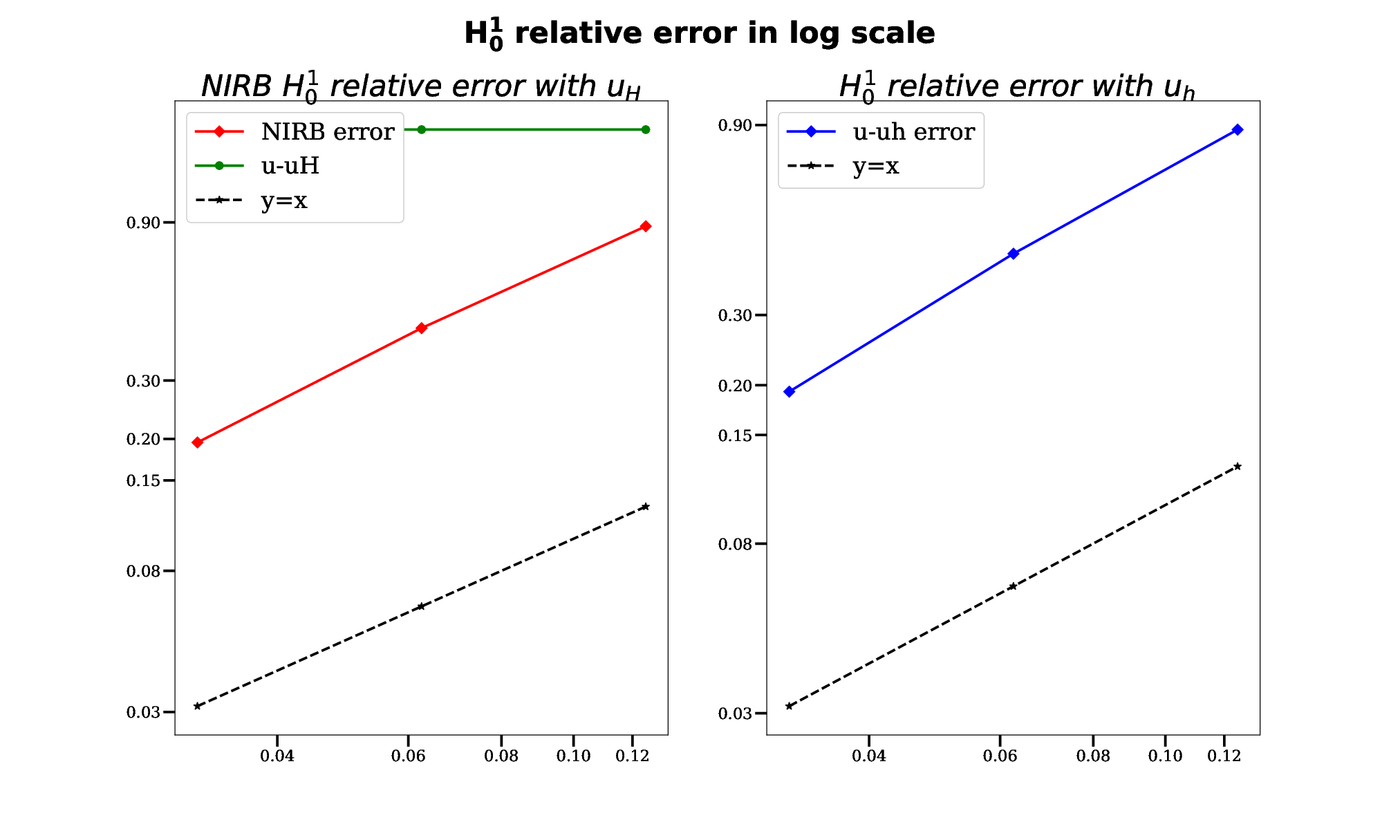
We consider two simple cases in 2D for the numerical results based with the TPFA scheme. Both results are computed on the unit square. We use an harmonic averaging of the diffusion coefficient( [17] section 5.3). Our variable parameter is $\mu\in\mathbb{R}^{4}=(\mu_{1},\mu_{2},\mu_{3},\mu_{4})$ . For both cases, the size of mesh $h$ is defined as the maximum length of the edges. The diffusion coefficient we consider here is $A(\mu)=(2\mu_{1}+\mu_{2}\sin(x+y)\cos(xy))$ and $f=(\mu_{3}(1-y)+\mu_{4}x(1-x))$ . We choose random coefficients for the snapshots with $N=5$ and our solution is defined with $\mu_{1}=0.99,\ \mu_{2}=0.8,\ \mu_{3}=0.2,\ \mu_{4}=0.78$ . For the exact solution, we consider the TPFA solution on a finer mesh (Figures 2, 4). For the computation of the norm, we use the discrete semi-norm as in the remark of the section 1 (10). NIRB results are compared to the classical finite volume error (Figures 3, 5). We measure the following relative error

\frac{\mathinner{\!\left\lVert u(\mu)-u_{Hh}^{N}(\mu)\right\rVert}_{\mathcal{T},2}}{\mathinner{\!\left\lVert u(\mu)\right\rVert}_{\mathcal{T},2}}.

(70)

Uniform grid

The first case presents results on a rectangular uniform grid where $\textbf{x}_{K}$ is the center of mass of the cell.

Refer to caption — Figure 2: coarse and fine solution with the uniform grid

Triangular mesh

The second case is defined on a triangular mesh where $\textbf{x}_{K}$ are the circumcenter of the cells, such that $e_{\mathfrak{G}}$ is in $\mathcal{O}(H^{2})$ .

Discussion on the implementation

We implemented the TPFA scheme on Scilab and retrieved several solutions for the NIRB algorithm on Python to highlight the black box side of the solver.

•

Implementation of TPFA
The TPFA on $\mathcal{T}_{h}$ reads: Find $u_{h}=(u_{K})_{K\in\mathcal{M}}$ such that:

\forall K\in\mathcal{M}_{h},\underset{\sigma\in\mathcal{F}_{K}\cap\mathcal{F}_{int}}{\sum}\tau_{\sigma}(u_{K}-u_{L})+\underset{\sigma\in\mathcal{F}_{K}\cap\mathcal{F}_{ext}}{\sum}\tau_{\sigma}u_{K}=\int_{K}f(\textbf{x})d\textbf{x},

(71)

where the harmonic average $\tau_{\sigma}=|\sigma|\frac{A(\textbf{x}_{L};\mu)A(\textbf{x}_{K};\mu)}{A(\textbf{x}_{L};\mu)\times d_{L,\sigma}+A(\textbf{x}_{K};\mu)\times d_{K,\sigma}}$ on $\mathcal{F}_{int}$ , and $\tau_{\sigma}=|\sigma|\frac{A(\textbf{x}_{K};\mu)}{d_{K,\sigma}}$ on $\mathcal{F}_{ext}$ .

To assemble the matrices $A$ of the TPFA scheme, we iterate on each edge, and we add the harmonic average $\tau_{\sigma}$ on each cell, and for $b$ we add the term $|D_{K,\sigma}|\times f(x_{K})$ .

•

Time execution (min,sec)

NIRB Online FV solver

uniform grid 00:06 01:48

triangular mesh 00:05 01:15

Remark 5.1.

Note that for the discontinuous diffusion coefficient $A$ , with the TPFA scheme, we recovered numerically the same estimate as in the Lipschitz continuous case, when we use the harmonic mean even if the proof no longer works.

Acknowledgements

This work is supported by the FUI MOR_DICUS. We would like to give special thanks to Nora Aïssiouene at the LJLL for her precious help.

References

[1] M. Barrault, C. Nguyen, A. Patera, and Y. Maday. An ‘empirical interpolation’ method: application to efficient reduced-basis discretization of partial differential equations. Comptes rendus de l’Académie des sciences. Série I, Mathématique, 339-9:667–672, 2004.
[2] F. Boyer. An introduction to finite volume methods for diffusion problems. French-Mexican Meeting on Industrial and Applied Mathematics Villahermosa, Mexico, November 25-29 2013.
[3] S. Brenner and R. Scott. The mathematical theory of finite element methods, volume 15. Springer Science & Business Media, 2007.
[4] F. Brezzi, K. Lipnikov, and M. Shashkov. Convergence of the mimetic finite difference method for diffusion problems on polyhedral meshes. SIAM Journal on Numerical Analysis, 43(5):1872–1896, 2005.
[5] A. Buffa, Y. Maday, A. T. Patera, C. Prud’homme, and G. Turinici. A priori convergence of the greedy algorithm for the parametrized reduced basis method. ESAIM: Mathematical Modelling and Numerical Analysis-Modélisation Mathématique et Analyse Numérique, 46(3):595 – 603, 2012.
[6] Fabien Casenave, Alexandre Ern, and Tony Lelièvre. A nonintrusive reduced basis method applied to aeroacoustic simulations. Advances in Computational Mathematics, 41(5):961–986, Jun 2014.
[7] R. Chakir. Contribution à l’analyse numérique de quelques problèmes en chimie quantique et mécanique. PhD thesis, 2009. Doctoral dissertation.
[8] R. Chakir, P. Joly, Y. Maday, and P. Parnaudeau. A non intrusive reduced basis method: application to computational fluid dynamics. 2013, September.
[9] R. Chakir, Y. Maday, and P. Parnaudeau. A non-intrusive reduced basis approach for parametrized heat transfer problems. Journal of Computational Physics, 376:617–633, 2019.
[10] A. Cohen and R. DeVore. Approximation of high-dimensional parametric pdes. arXiv preprint arXiv:1502.06797, 2015.
[11] L. B. da Veiga, K. Lipnikov, and G. Manzini. The mimetic finite difference method for elliptic problems, volume 11. Springer, 2014.
[12] D. A. Di Pietro, A. Ern, and S. Lemaire. An arbitrary-order and compact-stencil discretization of diffusion on general meshes based on local reconstruction operators. Computational Methods in Applied Mathematics, 14(4):461–472, 2014.
[13] J. Droniou. Finite volume schemes for diffusion equations: Introduction to and review of modern methods. Mathematical Models and Methods in Applied Sciences, 24 (8):1575–1619, 2014.
[14] J. Droniou and R. Eymard. A mixed finite volume scheme for anisotropic diffusion problems on any grid. Numerische Mathematik, 105(1):35–71, 2006.
[15] J. Droniou, R. Eymard, T. Gallouet, and R. Herbin. Gradient schemes: a generic framework for the discretisation of linear, nonlinear and nonlocal elliptic and parabolic equations. Mathematical Models and Methods in Applied Sciences, 23(13):2395–2432, 2013.
[16] J. Droniou, R. Eymard, T. Gallouët, C. Guichard, and R. Herbin. The gradient discretisation method. Springer, 82, 2018.
[17] J. Droniou, R. Eymard, T. Gallouët, and R. Herbin. A unified approach to mimetic finite difference, hybrid finite volume and mixed finite volume methods. Mathematical Models and Methods in Applied Sciences, 20(02):265–295, 2010.
[18] J. Droniou and N. Nataraj. Improved $l^{2}$ estimate for gradient schemes and super-convergence of the tpfa finite volume scheme. 3:1254–1293, 2017.
[19] R. Eymard, T. Gallouët, and R Herbin. Discretization schemes for linear diffusion operators on general non-conforming meshes. Finite volumes for complex applications V, pages 375–382, 2008.
[20] B. Haasdonk and M. Ohlberger. Reduced basis method for explicit finite volume approximations of nonlinear conservation laws. In Proc. 12th International Conference on Hyperbolic Problems: Theory, Numerics, Application. Citeseer, 2008.
[21] Jan S Hesthaven, Gianluigi Rozza, Benjamin Stamm, et al. Certified reduced basis methods for parametrized partial differential equations. Springer, 2016.
[22] O. Iliev, Y. Maday, and T. Nagapetyan. A Two-grid Infinite-volume/reduced Basis Scheme for the Approximation of the Solution of Parameter Dependent PDE with Applications the AFFFF Devices. Citeseer, 2013.
[23] A. Kolmogoroff. Über die beste annaherung von funktionen einer gegebenen funktionenklasse. Annals of Mathematics, pages 107–110, 1936.
[24] Y. Maday and R. Chakir. A two-grid finite-element/reduced basis scheme for the approximation of the solution of parametric dependent p.d.e. 2009.
[25] A. Quarteroni, A. Manzoni, and F. Negri. Reduced basis methods for partial differential equations: an introduction. Springer, 92, 2015.
[26] A. Quarteroni and S. Quarteroni. Numerical models for differential problems, volume 2. Springer, 2009.
[27] R. Sanchez. Application des techniques de bases réduites à la simulation des écoulements en milieux poreux. Université Paris-Saclay - CentraleSupélec, 2017.
[28] G. Stabile, S. Hijazi, A. Mola, S. Lorenzi, and G. Rozza. Pod-galerkin reduced order methods for cfd using finite volume discretisation: vortex shedding around a circular cylinder. Communications in Applied and Industrial Mathematics, 8(1):210–236, 2017.
[29] K. Veroy, C. Prud’Homme, and A. T. Patera. Reduced-basis approximation of the viscous Burgers equation: rigorous a posteriori error bounds. Comptes rendus de l’Académie des sciences. Série I, Mathématique, 337(9):619–624, November 2003.

$\displaystyle\left\rvert\underset{K\in\mathcal{M}_{H}}{\sum}\Phi_{i}(\textbf{x}_{K})\|K\|\Big[Q_{K}u(\overline{\textbf{x}}_{K};\mu)-Q_{K}u(\textbf{x}_{K};\mu)\Big]\right\rvert$	$\displaystyle\lesssim\left\rvert\underset{K\in\mathcal{M}_{H}}{\sum}\Big[\Phi_{i}(\textbf{x}_{G})+(\Phi_{i}(\textbf{x}_{K})-\Phi_{i}(\textbf{x}_{G}))\Big]\|K\|\Big[Q_{K}u(\overline{\textbf{x}}_{K};\mu)-Q_{K}u(\textbf{x}_{K};\mu)\Big]\right\rvert,$
	$\displaystyle\lesssim\left\rvert\underset{K\in\mathcal{M}_{H}}{\sum}\Phi_{i}(\textbf{x}_{G})\|K\|\Big[Q_{K}u(\overline{\textbf{x}}_{K};\mu)-Q_{K}u(\textbf{x}_{K};\mu)\Big]\right\rvert$
	$\displaystyle+\mathinner{\!\left\lVert\nabla\Phi_{i}\right\rVert}_{L^{\infty}(\Omega)}\underset{K\in\mathcal{M}_{H}}{\sum}H_{K}\|K\|\left\rvert Q_{K}u(\overline{\textbf{x}}_{K};\mu)-Q_{K}u(\textbf{x}_{K};\mu)\right\rvert\textrm{ since diam($U_{G}$) $\leq\mu_{G}H_{K}$ }.$	(57)

	$\displaystyle\left\rvert\underset{K\in\mathcal{M}_{H}}{\sum}\Phi_{i}(\textbf{x}_{G})\|K\|\Big[Q_{K}u(\overline{\textbf{x}}_{K};\mu)-Q_{K}u(\textbf{x}_{K};\mu)\Big]\right\rvert$	$\displaystyle\leq\left\rvert\underset{G\in\mathfrak{G}}{\sum}\underset{K\in G}{\sum}\Phi_{i}(\textbf{x}_{G})\frac{\|K\|}{\|B_{K}\|}\int_{B_{K}}D^{1}u(\mathbf{y})\cdot\mathbf{e}_{K}\ d\mathbf{y}\right\rvert,$
		$\displaystyle\leq\underset{G\in\mathfrak{G}}{\sum}\mathinner{\!\left\lVert\Phi_{i}\right\rVert}_{L^{\infty}(G)}\left\rvert\underset{K\in G}{\sum}\Big(\frac{1}{\|B_{K}\|}\int_{B_{K}}D^{1}u(\mathbf{y})\ d\mathbf{y}\Big)\|K\|\ \mathbf{e}_{K}\right\rvert.$		(58)

$\displaystyle\mathinner{\!\left\lVert\nabla\Phi_{i}\right\rVert}_{L^{\infty}(\Omega)}\underset{K\in\mathcal{M}_{H}}{\sum}H_{K}\|K\|\left\rvert Q_{K}u(\overline{\textbf{x}}_{K};\mu)-Q_{K}u(\textbf{x}_{K};\mu)\right\rvert$	$\displaystyle=\mathinner{\!\left\lVert\nabla\Phi_{i}\right\rVert}_{L^{\infty}(\Omega)}\underset{K\in\mathcal{M}_{H}}{\sum}H_{K}\frac{\|K\|}{\|B_{K}\|}\left\rvert\int_{B_{K}}D^{1}u(\mathbf{y})\cdot\mathbf{e}_{K}\ d\mathbf{y}\right\rvert,$
	$\displaystyle\lesssim\mathinner{\!\left\lVert\nabla\Phi_{i}\right\rVert}_{L^{\infty}(\Omega)}\underset{K\in\mathcal{M}_{H}}{\sum}H_{K}^{2}\mathinner{\!\left\lVert\nabla u\right\rVert}_{L^{1}(B_{K})},\textrm{ since $\|B_{K}\|\geq\theta_{H}^{-1}\|K\|$ \eqref{reg}},$
	$\displaystyle\leq H^{2}\mathinner{\!\left\lVert\nabla\Phi_{i}\right\rVert}_{L^{\infty}(\Omega)}\mathinner{\!\left\lVert\nabla u\right\rVert}_{L^{1}(\Omega)}.$	(59)

$\displaystyle\underset{G\in\mathfrak{G}}{\sum}\mathinner{\!\left\lVert\Phi_{i}\right\rVert}_{L^{\infty}(G)}\left\|\underset{K\in G}{\sum}\Big(\frac{1}{\|B_{K}\|}\int_{B_{K}}D^{1}u(\mathbf{y})\ d\mathbf{y}\Big)\|K\|\ \mathbf{e}_{K}\right\|$	$\displaystyle\leq\underset{G\in\mathfrak{G}}{\sum}\mathinner{\!\left\lVert\Phi_{i}\right\rVert}_{L^{\infty}(G)}\Big\|\underset{K\in G}{\sum}\Big(\left\|\frac{1}{\|B_{K}\|}\int_{B_{K}}D^{1}u(\mathbf{y})\ d\mathbf{y}-\ \frac{1}{\|K\|}\int_{K}D^{1}u(\mathbf{y};\mu)\ d\mathbf{y}\right\|$
	$\displaystyle+\ \left\|\frac{1}{\|K\|}\int_{K}D^{1}u(\mathbf{y};\mu)\ d\mathbf{y}\ -\ \frac{1}{\|B_{G}\|}\int_{B_{G}}D^{1}u(\mathbf{y};\mu)\ d\mathbf{y}\right\|$
	$\displaystyle+\left\|\frac{1}{\|B_{G}\|}\int_{B_{G}}D^{1}u(\mathbf{y};\mu)\ d\mathbf{y}\ -\ \frac{1}{\|U_{G}\|}\int_{U_{G}}D^{1}u(\mathbf{y};\mu)\ d\mathbf{y}\right\|$
	$\displaystyle+\frac{1}{\|U_{G}\|}\int_{U_{G}}D^{1}u(\mathbf{y};\mu)\ d\mathbf{y}\Big)\ \|K\|\ \mathbf{e}_{K}\Big\|.$	(62)

	$\displaystyle\underset{G\in\mathfrak{G}}{\sum}\mathinner{\!\left\lVert\Phi_{i}\right\rVert}_{L^{\infty}(G)}\left\|\underset{K\in G}{\sum}\Big(\frac{1}{\|B_{K}\|}\int_{B_{K}}D^{1}u(\mathbf{y})\ d\mathbf{y}\Big)\|K\|\ \mathbf{e}_{K}\right\|$	$\displaystyle\lesssim\underset{G\in\mathfrak{G}}{\sum}\mathinner{\!\left\lVert\Phi_{i}\right\rVert}_{L^{\infty}(G)}\Big\|\underset{K\in G}{\sum}\Big(\mathinner{\!\left\lVert u\right\rVert}_{W^{2,1}(U_{G})}\textrm{diam}(U_{G})^{d}\Big[\frac{\textrm{diam}(U_{G})}{\|B_{K}\|\|K\|}$
		$\displaystyle+\frac{\textrm{diam}(U_{G})}{\|B_{G}\|\|K\|}+\frac{\textrm{diam}(U_{G})}{\|U_{G}\|\|B_{G}\|}\Big]+\frac{1}{\|U_{G}\|}\int_{U_{G}}D^{1}u(\mathbf{y};\mu)\ d\mathbf{y}\Big)\ \|K\|\ \mathbf{e}_{K}\Big\|.$		(63)