Gauging diffraction patterns: field of view and bandwidth estimation in lensless holography

Throughout this paper, we use lower case letters for functions and scalars (e.g. $o$ and $\lambda$), boldface lowercase letters for vectors (e.g. $\boldsymbol{o}$) upper case calligraphic letters for operators acting on functions (e.g. $\mathcal{M}$) and boldface uppercase letters for matrices (e.g. $\mathbf{H}$). $\boldsymbol{x}^{\top}$ is the adjoint (i.e. the conjugate transpose) of $\boldsymbol{x}$. $\left\|\boldsymbol{x}\right\|_{2}=\sqrt{\boldsymbol{x}^{\top}\boldsymbol{x}}$ is the Euclidean norm of $\boldsymbol{x}$. $\boldsymbol{x}^{\top}\boldsymbol{y}$ is the scalar product t between vectors $\boldsymbol{x}$ and $\boldsymbol{y}$ and $\boldsymbol{x}\,\times\boldsymbol{y}$ their element-wise product.

With these notations, each wave is represented by a square integrable 2D function from $\mathbb{R}^{2}$ to $\mathbb{C}$ (e.g. $w\,:\,\mathbb{R}^{2}\rightarrow\mathbb{C}$) and with lateral coordinates $\boldsymbol{x}=[x_{1},x_{2}]^{\top}$. The discretized version of this wave is the vector $\boldsymbol{w}$ ordered in lexicographical order (e.g. $\boldsymbol{w}=[w_{1},\dots,w_{N}]^{\top}$ where $N$ is the number of pixels). Functions and vectors with a hat (e.g. $\widehat{w}$) and without a hat (e.g. $w$) are in Fourier domain and space domain respectively.

”We consider the lensless setup depicted in Fig. 1: a thin (2D) sample, described by the function $o\,:\,\mathbb{R}^{2}\rightarrow\mathbb{C}$, is placed orthogonally to the optical axis at $z=0$. It is illuminated by a plane wave of wavelength $\lambda$ (or a wavenumber $k=n\frac{2\,\pi}{\lambda}$) arriving with an incidence angle $\boldsymbol{\theta}=[\theta_{1},\theta_{2}]^{\top}$ relatively to the optical axis. After propagation in a medium of refractive index $n$, the diffracted wave $w$ is recorded by a detector of size $\ell_{1}\times\ell_{2}$ placed at a distance $z$, orthogonally to the optical axis. The detector produces the discrete measurements $\boldsymbol{d}\in\mathbb{R}^{N}$.

To give a correct interpretation of the measurements $\boldsymbol{d}$, one has to derive a rigorous model accounting for the totality of the measured information. This is summed up by building the forward operator $\mathcal{M}:\,L^{2}(\mathbb{R}^{2})\to\mathbb{R}^{N}$ acting on the Hilbert space of squared integrable functions $L^{2}$ and linking the object $o$ to the measurements $\boldsymbol{d}\in\mathbb{R}^{N}$:

where $\boldsymbol{e}$ is an error term.

In lensless holography, this forward operator can be described as the composition of three operators:

where $\mathop{\circ}$ denotes the composition and:

• •

  $\mathcal{H}:\,L^{2}(\mathbb{R}^{2})\to L^{2}(\mathbb{R}^{2})$ models the light propagation from the sample plane to the detector plane. This linear operator is described in Sec. 2.2.

• •

  $\mathcal{C}:\,L^{2}(\mathbb{R}^{2})\to L^{2}(\mathbb{D})$ cuts the input function on the compact support $\mathbb{D}\subset\mathbb{R}^{2}$ describing the sensitive area of the detector of size $\boldsymbol{\ell}=[\ell_{1},\ell_{2}]^{\top}$:

  $\displaystyle\mathcal{C}(f)(\boldsymbol{x})$

  $\displaystyle=\left\{\begin{array}[]{ll}f(\boldsymbol{x})&\text{if }\boldsymbol{x}\in\,\mathbb{D}\,,\\ 0&\text{otherwise}\,.\end{array}\right.$

• •

  $\mathcal{S}:\,L^{2}(\mathbb{D})\to\mathbb{R}_{+}^{N}$ models the sensing and the sampling performed by a detector with $N$ pixels. In inline holography, the detector samples the intensity of the scattered wave.

Right after the interaction of the illumination wave with the sample $o$, the complex wave field $v$ is:

where $\sin(\boldsymbol{\theta})=[\sin(\theta_{1}),\sin(\theta_{2})]^{\top}$ is the component wise 2D sine. It can be expressed as a shift in the Fourier domain:

where $\boldsymbol{\omega}=[\omega_{1},\omega_{2}]^{\top}\in\mathbb{R}^{2}$ is the 2D angular frequency and $\mathcal{F}$ is the continuous (non unitary) 2D Fourier transform operator defined as:

The property of shifting the sample’s Fourier spectrum by a tilted illumination can be used to perform aperture synthesis as in Fourier ptychography[44].

Given the high numerical aperture of a lensless setup, the propagation is modeled in the near-field regime by the mean of the angular spectrum (AS) propagation mode [8]. It gives the Fourier transform of the complex wave field $w$ in the detector plane as:

where $\widehat{f}^{\mathrm{AS}}$ is the angular spectrum transfer function for $z\gg\lambda$ (neglecting evanescent waves) [8]:

Let us note here that when most of the propagating wave energy is concentrated on low angular frequencies, the propagation kernel is non null only when $\left\|\boldsymbol{\omega}\right\|^{2}\ll k^{2}$ leading to the approximation $\sqrt{k^{2}-\left\|\boldsymbol{\omega}\right\|^{2}}\approx k-\frac{\left\|\boldsymbol{\omega}\right\|^{2}}{2\,k}$. This is the paraxial approximation and, discarding the constant term $\mathrm{e}^{\jmath\,k\,z}$, the propagation kernel becomes the Fresnel transfer function:

The wave field in the detector plane $w$ can be rewritten in the space domain expressing the operator $\mathcal{H}$ as:

where $\widehat{h}$ is the shifted angular spectrum transfer function [45]:

Its expression in space is the Hyugens-Fresnel convolution kernel [8] under oblique illumination [45]:

The Wigner distribution function $W^{\mathrm{F}}$ of the Fresnel transfer function given Eq. (10) is [49]:

where $\widehat{f}^{\mathrm{F*}}$ is the complex conjugate of $\widehat{f}^{\mathrm{F}}$ and $\delta$ the Dirac delta function.

As a multiplication in Fourier domain is a convolution along the space dimension in the Wigner domain, the Fresnel propagation corresponds to a horizontal shearing of the signal SBP [50] as depicted in Fig. 2.b. As stated in [23], to prevent loss of information, the propagated signal must be sampled on an area of width $\ell_{s}+z\,\frac{B_{s}}{k}$ that encompasses all its support in the Wigner domain.

Conversely, as in practice the propagated signal is sampled on a rectangular area in the Wigner domain of width $\ell$, the lensless holographic setup probe a region of the sampled sheared in the opposite direction as depicted on the dark grey area of Fig. 3. This means that under Fresnel approximation for a band-limited sample of angular bandwidth $B_{s}$, the FoV of a setup with a detector of width $\ell$ is $\ell_{1}^{\mathrm{F}}\times\ell_{2}^{\mathrm{F}}$ with:

As a consequence of the shearing of the space-bandwidth product, the bandwidth and thus the resolution of a lensless setup varies within the FoV [25, 26, 27]. The resolution is coarser at the center (with a resolution of $r_{\textrm{center}}=\frac{\lambda\,z}{2\,\ell}$ at best) than on the edges of the FoV (resolution of $r_{\textrm{edge}}=\frac{4\,\pi}{B_{s}}$ at best).

Wigner distribution function of the angular spectrum kernel Eq. (9) is impossible to estimate analytically. However, its support in the Wigner domain can be estimated using the instantaneous frequency of the angular spectrum kernel expressed in space Eq. (14):

where $\mathop{\operator@font Arg}\nolimits(h)$ is the complex argument of ${h}$ and $\xi_{i}(\boldsymbol{x})$ is the instantaneous frequency along the dimension $i$ and at the position $\boldsymbol{x}$. In 1D (taking $x=x_{1}$ and $x_{2}=0$):

The propagation kernel $h$ is a chirp and its instantaneous frequency increases monotonically with $x$. This means that the probed bandwidth of a lensless setup varies within the FoV. At a given position in the sample plane, the bandwidth probed by the setup is bounded by the instantaneous frequencies at each edges of the sensor. As a consequence, the SBP of a lensless setup is the area between $\xi(x+\frac{\ell}{2})$ and $\xi(x-\frac{\ell}{2})$ as depicted Fig. 3. It is:

that corresponds to a number of degrees of freedom of $2\,\frac{\ell}{\lambda}$: the highest number of degrees of freedom it is physically possible to record on a detector of size $\ell$. The incidence angle shifts the SBP along the angular frequency axis without changing its shape. The center of the FoV $\boldsymbol{x}^{c}$ is given by:

as it is expected from geometrical optics.

For low spatial frequencies (i.e. within the paraxial approximation), SBP of AS and Fresnel (in dark gray on Fig. 3) are identical.

To perfectly explain the propagated wave in the detector plane, one has to model the sampled a rectangular area in the Wigner domain that encompasses all the SBP of the angular spectrum. That is on a bandwidth of $B=2\,k$ centered on $k\,\sin(\theta)$. Along the space dimension, this SBP spans the whole axis implying an infinite FoV: $\ell^{\mathrm{AS}}=\infty$. This is a consequence of the infinite size in space of the AS kernel Eq. (14).

Assessing the size of the propagation kernel in space also amounts to estimate the smallest sampling rate of the Fourier space needed to perfectly sample $\widehat{h}^{\mathrm{AS}}$. It is estimated by computing its highest instantaneous frequencies along both dimension:

The instantaneous frequency $\tau_{1}$ (resp. $\tau_{2}$) is infinite for $\omega_{1}=k\,\left(\mathop{\operator@font sign}\nolimits(\theta_{1})+\sin(\theta_{1})\right)$ (resp. $\omega_{2}=k\,\left(\mathop{\operator@font sign}\nolimits(\theta_{2})+\sin(\theta_{2})\right)$). The diffraction patterns are thus infinitely extended in the detector plane highlighting the bandlimited nature of $\widehat{h}^{\mathrm{AS}}$. However, $\widehat{h}^{\mathrm{AS}}$ is still approximately well sampled as long as the phase difference of $\widehat{h}^{\mathrm{AS}}$ between two consecutive frequels is lower than $\pi$ [51]. This is true when the FoV $\ell^{\prime}\times\ell^{\prime}$ verifies :

The theoretical FoV given by Eq. (25) is too large, much larger than the effective FoV of the setup in practice. As an example, $\ell^{\prime}=3\,$m for the parameters used in [3]: $\lambda=681\,$nm and $z=1.02\,$mm. However several physical phenomena decrease the size of diffraction pattern detectable in practice, narrowing the FoV.

The extent of the diffraction kernel can be defined as the area where its intensity is over the detector detection limits. This can be characterized as the distance $p$ from the center of a diffraction kernel after which the fringes are no longer detectable by the sensor.

In the detector plane, the contrast of a diffraction pattern decreases with the distance from its center. As it scatters more power, the larger the object is, the wider its diffraction pattern is. The largest diffraction pattern is given by a half plane:

Along the $x_{1}$ axis, the diffraction by a half plane under inclined illumination is given by [52]:

where $(r,\alpha)$ are polar coordinates as depicted on Fig. 4. $F$ is the Fresnel integral under the form:

The geometrical shadow of the edge is $x_{c}=z\,\tan(\theta)$ and its distance from the edge is $r_{c}=z/\cos(\theta)$. In an in-line setup, the intensity for $t>0$ ($\alpha>0$) is approximately bounded by (see Fig. 5 for two examples) :

The half-width of the diffraction pattern to the left $p^{-}$ is the distance $t$ from $x_{c}$ after which the fringes are no longer detectable. The threshold $\eta$ below which the fringes are no longer visible is defined as the smallest effective quantification level relatively to illumination mean intensity $I_{0}$.

where $\sigma$ is the mean standard deviation of the noise and $\zeta$ is the quantification level of the camera. The half-width of the diffraction pattern to the right $p^{+}$ is given by the symmetry with respect to the sensor (that is changing the sign of $\theta$). As the bound in Eq. (32) depends only on $|\theta|$, we have $p_{i}^{+\mathrm{noise}}=p_{i}^{-\mathrm{noise}}=p_{i}^{\mathrm{noise}}$. Given the threshold $\eta$, the half-width of the diffraction pattern along dimension $i$ is $p_{i}^{\mathrm{noise}}$, such that:

As an example, for the parameters used in [3] ($\lambda=681\,$nm and $z=1.02\,$mm, $\theta_{1}=9^{\circ}$) and a camera of width $\ell_{1}=5.3\,\textrm{mm}$ and $20\,$dB of noise ($\eta=10^{-2}$), the estimated bound is $p_{i}^{\mathrm{noise}}=911$µm leading to a width of the field of view of $\ell_{1}^{\prime}=7.1\,\textrm{mm}$ much more tractable than $\ell^{\prime}=3\,\textrm{m}$ given by Eq. (25).

Let us notice that in detection applications such as [24] scatterers can be detected in an even larger FoV as the noise is averaged on a large number of pixels increasing the effective $\mathrm{SNR}$.

In the previous sections, we always consider illumination light as a single monochromatic plane wave. However, in practice any real source must have a finite size and a finite spectral bandwidth. This partial coherence affects the size of the diffraction patterns as it decreases the visibility of the fringes and blurs out intensity high spatial frequencies. As the spatial frequencies of the fringes increase with the distance from the center of the diffraction pattern, this effectively reduces its extent. It is possible to assess the extension of the diffraction pattern by considering the Born approximation model of inline holography where the diffraction pattern is generated by the interferences between the illumination wave $v_{i}$ and the wave $v_{d}$ diffracted by a scatterer P as depicted on Fig. 6. On the detector plane, at a distance $\boldsymbol{\Delta}=[\Delta_{1},\Delta_{2}]^{\top}$ from the center of the diffraction pattern, the coherence of these two waves can be described by their mutual coherence factor [53] :

where $\left\langle v(t)\right\rangle_{t}$ is the average over time. When $\boldsymbol{\Delta}=0$ (at the center of the diffraction pattern) illumination wave and diffracted wave coincide and $\left|\mu(\boldsymbol{\Delta})\right|$ is maximum. When $\left|\mu(\boldsymbol{\Delta})\right|=0$ the two waves are mutually incoherent and no longer interfere.

To simplify further computations, we set an upper bound estimate on $\mu(\boldsymbol{\Delta})$ that is separable along both lateral axis giving the maximal possible extension of the diffraction pattern:

Along dimension $i$, the coherence factor $\mu_{i}(\Delta_{i})$ can be inferred from both spectral and spatial coherence of the illumination wave (supposed quasi-homogeneous [53]) given by its complex degree of coherence :

Using the notation given on Fig. 6, the distance between P and A is $\delta_{i}^{AP}=\frac{\Delta_{i}}{\cos{(\theta_{i})}}$ the relative time delay between B and A (for $v_{i}$), and P and B (for $v_{d}$) are:

This gives the mutual coherence factor between $v_{i}$ and $v_{d}$ at position $\Delta_{i}$:

This relation will be used to determine the half-width of the diffraction pattern in the two limiting cases: (i) a spatially coherent illumination ($\gamma({\delta},\tau)=\gamma(0,\tau),\ \forall{\delta}$ ) and (ii) a spatially incoherent quasi-monochromatic illumination ($\gamma({\delta},\tau)=\gamma({\delta},0),\ \forall{\tau}$ ).

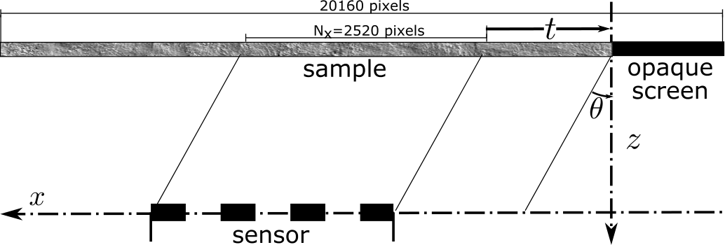
We now illustrate the usefulness of the bounds derived in the previous sections on simulations. We define a reference intensity $\boldsymbol{r}$ with suitable noise and coherence properties. This reference is established by simulating the propagation over a large FoV of $20160\times 20160$ pixels while computing the modeling error $E$ in each experiments on a much smaller area ($2520\times 2520$ pixels). The effect of partial coherence is simulated using a Monte-Carlo method.

In all experiments, we plot the modeling error $E(t)$ (in dB) between this reference $\boldsymbol{r}$ and the intensity $\boldsymbol{s}$ computed when part of the sample is zeroed by an opaque screen as depicted on Fig. 8. The intensity $\boldsymbol{s}(t)$ is simulated by propagating the masked sample exactly as the reference $\boldsymbol{r}$ but without noise and coherence effects. This error $E$ is computed as a function of the lateral distance $t$ of the screen to the edge of the sensor projected at the sample depth parallel to the illumination incidence. It is normalized by the error for the intensity computed without the screen $\boldsymbol{s}_{\infty}$ (or when $t$ is very large):

This error is maximum when $t=0$ showing the modeling error made when the FoV it restricted to the size of the sensor and goes to $0$ as $t$ increase.

For each experimental condition the measured modeling error $E(t)$ is averaged over many experiments with different objects and noise realizations. We use 5 different images that were randomly shifted to generate dozens of images used in simulations. These images¹¹ 1 All images are available at https://doi.org/10.6084/m9.figshare.7998143 and https://doi.org/10.6084/m9.figshare.7998134 are shown on Fig. 9. Three of these were built using very large images eventually padded with mirror boundaries to the size $20160\times 20160$ pixels. One pure phase and one pure transmittance object were built from vector graphic defined USAF-1951 resolution target discretized at the right resolution. The propagation is perform with pixels of size $104\,\textrm{nm}<\lambda/4$ to ensure that no aliasing occurs in the intensity modeling. From the object plane to the detector plane, the propagation was modeled using BLAS (Band-Limited Angular Spectrum) model [33] that implements a version of the angular spectrum propagation kernel filtered to prevent aliasing. As all the propagations are performed over the same large FoV and with the same small pixel-size, this filtering has no influence on our estimations. The physical parameters used all experiments are given in Tab.1. All numerical experiments were implemented²² 2 code available on https://github.com/FerreolS/COMCI within the framework of the GlobalBioIm library [54].

To assess the quality of the bounds derived in Sec. 4 for i.i.d. Gaussian noise, the modeling error $E(t)$ is estimated for two cases: (i) for a fixed noise level and varying the incidence angle, (ii) for a fixed incidence angle and varying the noise level. All the curves are computed by averaging the error over 100 different simulations.

Figure 10 shows the modeling error for incidence angles of $\theta_{1}=[0^{\circ},30^{\circ},45^{\circ},60^{\circ}]$ and a noise level of $20\,$dB. As the width of the diffraction pattern is independent of the sign of the incidence angle, negative incidence would have produces similar curves. Figure 11 shows the modeling error for an incidence angle of $\theta_{1}=45^{\circ}$ and noise level of $[6,14,20,26]$ dB. The bounds derived in Eq. (35) are plotted on these figures. They are approximately at the bend of each plot and provide a good trade-off between the size of the FoV and the modeling error.

The effect of a finite temporal coherence on the reference $\boldsymbol{r}$ is computed using Monte-Carlo method averaging 100 intensities in the sensor plane for wavelengths drawn under a Normal law modeling an illumination source with a Gaussian emission spectrum. Figure 12 shows the modeling error $E(t)$ for an incidence of $\theta_{1}=-30^{\circ}$ and several coherence lengths $L_{c}=[2,20,80]\,\text{\textmu{}m}$ typical of light sources used for digital holography (from white light to laser diode).

We simulate the reference $\boldsymbol{r}$ as the hologram of the sample illuminated by an uniformly bright incoherent quasi-monochromatic circular source. To that end, we model the effect of a finite spatial coherence using Monte-Carlo method averaging 100 intensities for illumination incidence drawn uniformly within the angular size of the source. Figure 13 shows the modeling error for a source placed at $\theta_{1}=-30^{\circ}$ and with different angular radius $\alpha=[0.05^{\circ},0.07^{\circ},0.2^{\circ}]$.

References

- [1] O. Mudanyali, D. Tseng, C. Oh, S. O. Isikman, I. Sencan, W. Bishara, C. Oztoprak, S. Seo, B. Khademhosseini, and A. Ozcan, “Compact, light-weight and cost-effective microscope based on lensless incoherent holography for telemedicine applications,” Lab on a Chip 10, 1417 (2010).
- [2] M. Rostykus, F. Soulez, M. Unser, and C. Moser, “Compact lensless phase imager,” Optics Express 25, 4438 (2017).
- [3] M. Rostykus, F. Soulez, M. Unser, and C. Moser, “Compact in-line lensfree digital holographic microscope,” Methods 136, 17–23 (2018).
- [4] C. P. Allier, G. Hiernard, V. Poher, and J. M. Dinten, “Bacteria detection with thin wetting film lensless imaging,” Biomedical Optics Express 1, 762 (2010).
- [5] O. Mudanyali, E. McLeod, W. Luo, A. Greenbaum, A. F. Coskun, Y. Hennequin, C. P. Allier, and A. Ozcan, “Wide-field optical detection of nanoparticles using on-chip microscopy and self-assembled nanolenses,” Nature Photonics 7, 247–254 (2013).
- [6] S. Murata and N. Yasuda, “Potential of digital holography in particle measurement,” Optics & Laser Technology 32, 567–574 (2000).
- [7] U. Schnars and W. Jüptner, “Direct recording of holograms by a CCD target and numerical reconstruction,” Applied Optics 33, 179 (1994).
- [8] J. Goodman, Introduction to Fourier Optics (Roberts and Company Publishers, 2004).
- [9] J. H. Milgram and W. Li, “Computational reconstruction of images from holograms,” Applied Optics 41, 853 (2002).
- [10] F. Dubois, O. Monnom, C. Yourassowsky, and J.-C. Legros, “Border processing in digital holography by extension of the digital hologram and reduction of the higher spatial frequencies,” Applied Optics 41, 2621 (2002).
- [11] A. Migukin, V. Katkovnik, and J. Astola, “Wave field reconstruction from multiple plane intensity-only data: augmented lagrangian algorithm,” Journal of the Optical Society of America A 28, 993 (2011).
- [12] T. Latychevskaia and H.-W. Fink, “Resolution enhancement in digital holography by self-extrapolation of holograms,” Optics Express 21, 7726 (2013).
- [13] W. Bishara, T.-W. Su, A. F. Coskun, and A. Ozcan, “Lensfree on-chip microscopy over a wide field-of-view using pixel super-resolution,” Optics Express 18, 11181 (2010).
- [14] J. Zhang, J. Sun, Q. Chen, J. Li, and C. Zuo, “Adaptive pixel-super-resolved lensfree in-line digital holography for wide-field on-chip microscopy,” Scientific Reports 7 (2017).
- [15] Z. Luo, A. Yurt, R. Stahl, A. Lambrechts, V. Reumers, D. Braeken, and L. Lagae, “Pixel super-resolution for lens-free holographic microscopy using deep learning neural networks,” Optics Express 27, 13581 (2019).
- [16] T. M. Kreis, M. Adams, and W. P. O. Jueptner, “Methods of digital holography: a comparison,” in “Optical Inspection and Micromeasurements II,” C. Gorecki, ed. (SPIE, 1997).
- [17] F. Soulez, L. Denis, É. Thiébaut, C. Fournier, and C. Goepfert, “Inverse problem approach in particle digital holography: out-of-field particle detection made possible,” Journal of the Optical Society of America A 24, 3708 (2007).
- [18] L. Denis, D. Lorenz, E. Thiébaut, C. Fournier, and D. Trede, “Inline hologram reconstruction with sparsity constraints,” Optics Letters 34, 3475 (2009).
- [19] C. Fournier, F. Jolivet, L. Denis, N. Verrier, E. Thiebaut, C. Allier, and T. Fournel, “Pixel super-resolution in digital holography by regularized reconstruction,” Applied Optics 56, 69 (2016).
- [20] A. Greenbaum, W. Luo, B. Khademhosseinieh, T.-W. Su, A. F. Coskun, and A. Ozcan, “Increased space-bandwidth product in pixel super-resolved lensfree on-chip microscopy,” Scientific Reports 3 (2013).
- [21] W. Luo, A. Greenbaum, Y. Zhang, and A. Ozcan, “Synthetic aperture-based on-chip microscopy,” Light: Science & Applications 4, e261–e261 (2015).
- [22] L. Onural, “Sampling of the diffraction field,” Applied Optics 39, 5929 (2000).
- [23] A. Stern and B. Javidi, “Improved-resolution digital holography using the generalized sampling theorem for locally band-limited fields,” Journal of the Optical Society of America A 23, 1227 (2006).
- [24] F. Soulez, L. Denis, C. Fournier, É. Thiébaut, and C. Goepfert, “Inverse-problem approach for particle digital holography: accurate location based on local optimization,” Journal of the Optical Society of America A 24, 1164 (2007).
- [25] C. Fournier, L. Denis, and T. Fournel, “On the single point resolution of on-axis digital holography,” Journal of the Optical Society of America A 27, 1856 (2010).
- [26] D. P. Kelly, “Resolution limits in practical digital holographic systems,” Optical Engineering 48, 095801 (2009).
- [27] Y. Hao and A. Asundi, “Resolution analysis of a digital holography system,” Applied Optics 50, 183 (2011).
- [28] T. E. Agbana, H. Gong, A. S. Amoah, V. Bezzubik, M. Verhaegen, and G. Vdovin, “Aliasing, coherence, and resolution in a lensless holographic microscope,” Optics Letters 42, 2271 (2017).
- [29] J. Zhang, J. Sun, Q. Chen, and C. Zuo, “Resolution analysis in a lens-free on-chip digital holographic microscope,” IEEE Transactions on Computational Imaging 6, 697–710 (2020).
- [30] N. Chacko, M. Liebling, and T. Blu, “Discretization of continuous convolution operators for accurate modeling of wave propagation in digital holography,” Journal of the Optical Society of America A 30, 2012 (2013).
- [31] D. P. Kelly, “Numerical calculation of the fresnel transform,” Journal of the Optical Society of America A 31, 755 (2014).
- [32] J.-P. Liu, “Controlling the aliasing by zero-padding in the digital calculation of the scalar diffraction,” Journal of the Optical Society of America A 29, 1956 (2012).
- [33] K. Matsushima and T. Shimobaba, “Band-limited angular spectrum method for numerical simulation of free-space propagation in far and near fields,” Optics Express 17, 19662 (2009).
- [34] K. Matsushima, “Shifted angular spectrum method for off-axis numerical propagation,” Optics Express 18, 18453 (2010).
- [35] S. Odate, C. Koike, H. Toba, T. Koike, A. Sugaya, K. Sugisaki, K. Otaki, and K. Uchikawa, “Angular spectrum calculations for arbitrary focal length with a scaled convolution,” Optics Express 19, 14268 (2011).
- [36] H. M. Ozaktas, S. Ö. Arık, and T. Coşkun, “Fundamental structure of fresnel diffraction: natural sampling grid and the fractional fourier transform,” Optics Letters 36, 2524 (2011).
- [37] K. Falaggis, T. Kozacki, and M. Kujawinska, “Computation of highly off-axis diffracted fields using the band-limited angular spectrum method with suppressed gibbs related artifacts,” Applied Optics 52, 3288 (2013).
- [38] T. Kozacki and K. Falaggis, “Angular spectrum-based wave-propagation method with compact space bandwidth for large propagation distances,” Optics Letters 40, 3420 (2015).
- [39] A. Ritter, “Modified shifted angular spectrum method for numerical propagation at reduced spatial sampling rates,” Optics Express 22, 26265 (2014).
- [40] T. Shimobaba, T. Kakue, N. Okada, M. Oikawa, Y. Yamaguchi, and T. Ito, “Aliasing-reduced fresnel diffraction with scale and shift operations,” Journal of Optics 15, 075405 (2013).
- [41] X. Yu, T. Xiahui, Q. Yingxiong, P. Hao, and W. Wei, “Band-limited angular spectrum numerical propagation method with selective scaling of observation window size and sample number,” Journal of the Optical Society of America A 29, 2415 (2012).
- [42] F. Gori, “Fresnel transform and sampling theorem,” Optics Communications 39, 293–297 (1981).
- [43] J. Liang and M. F. Becker, “Spatial bandwidth analysis of fast backward fresnel diffraction for precise computer-generated hologram design,” Applied Optics 53, G84 (2014).
- [44] G. Zheng, R. Horstmeyer, and C. Yang, “Wide-field, high-resolution fourier ptychographic microscopy,” Nature photonics 7, 739–745 (2013).
- [45] C.-S. Guo, Y.-Y. Xie, and B. Sha, “Diffraction algorithm suitable for both near and far field with shifted destination window and oblique illumination,” Optics Letters 39, 2338 (2014).
- [46] D. Mendlovic, A. W. Lohmann, and Z. Zalevsky, “Space–bandwidth product adaptation and its application to superresolution: examples,” Journal of the Optical Society of America A 14, 563 (1997).
- [47] A. Stern and B. Javidi, “Sampling in the light of wigner distribution,” Journal of the Optical Society of America A 21, 360 (2004).
- [48] D. Claus, D. Iliescu, and P. Bryanston-Cross, “Quantitative space-bandwidth product analysis in digital holography,” Applied Optics 50, H116 (2011).
- [49] A. W. Lohmann, R. G. Dorsch, D. Mendlovic, C. Ferreira, and Z. Zalevsky, “Space–bandwidth product of optical signals and systems,” Journal of the Optical Society of America A 13, 470 (1996).
- [50] A. W. Lohmann, “Image rotation, wigner rotation, and the fractional fourier transform,” Journal of the Optical Society of America A 10, 2181 (1993).
- [51] D. G. Voelz and M. C. Roggemann, “Digital simulation of scalar optical diffraction: revisiting chirp function sampling criteria and consequences,” Applied Optics 48, 6132 (2009).
- [52] C. J. R. Sheppard and M. Hrynevych, “Diffraction by a half-plane: a generalization of the fresnel diffraction theory,” Optics Letters 16, 1060 (1991).
- [53] J. W. Goodman, Statistical optics (John Wiley & Sons, 2015).
- [54] E. Soubies, F. Soulez, M. T. McCann, T.-a. Pham, L. Donati, T. Debarre, D. Sage, and M. Unser, “Pocket guide to solve inverse problems with GlobalBioIm,” Inverse Problems 35, 1–20 (2019).
- [55] D. H. Kelly, “Spatial frequency, bandwidth, and resolution,” Applied Optics 4, 435 (1965).