Conditional Frechet Inception Distance
Abstract
We consider distance functions between conditional distributions. We focus on the Wasserstein metric and its Gaussian case known as the Frechet Inception Distance (FID). We develop conditional versions of these metrics, analyze their relations and provide a closed form solution to the conditional FID (CFID) metric. We numerically compare the metrics in the context of performance evaluation of modern conditional generative models. Our results show the advantages of CFID compared to the classical FID and mean squared error (MSE) measures. In contrast to FID, CFID is useful in identifying failures where realistic outputs which are not related to their inputs are generated. On the other hand, compared to MSE, CFID is useful in identifying failures where a single realistic output is generated even though there is a diverse set of equally probable outputs.
I Introduction
Generative models have revolutionized the machine learning world by learning how to efficiently sample from an unknown distribution. Such models have become ubiquitous since the introduction of the seminal Generative Adversarial Network (GAN) [12]. Conditional GANs were then developed to sample from a conditional distribution [25]. Recent unsupervised training of models can even learn from an unpaired dataset when the inputs and outputs are not aligned [43, 31, 14, 3]. Every day new models are developed improving state of the art, such as speech-to-image translations [19]. Yet, it is still poorly understood how to measure their performance. There is a large body of works on unconditional metrics that help in comparing different models [23, 7]. Among these, the Frechet Inception Distance [13] (FID) has become a popular measure due to its simplicity. Perhaps surprisingly, it is also frequently used in the analysis of conditional generators, e.g., [30, 42, 19]. The goal of this work is therefore to introduce conditional versions of FID, develop the necessary machinery and examine it in different models and datasets.
Measuring the distance between two distributions is a fundamental problem in statistics. There are classical metrics based on likelihoods, divergences and other statistical notions, e.g. Kullback Leibler divergence (KLD) [32], Wasserstein distance (WD) [36], and total variation [36]. Each emphasizes various properties of the distributions with different sample and computational complexities. Unfortunately, modern applications involve huge dimensional datasets in which estimating these distances is difficult. Practical approaches consider simplified measures based on low dimensional embeddings, accuracy in some downstream task and/or some restricted parametric family. Arguably the most widely adopted metric in the computer vision literature is the Inception Score (IS) [33]. It is applicable for classification tasks and is based on the KLD of the labels. Another measure is based on “inference through optimization” where a nearest GAN sample is optimized per real sample [24]. It is also popular to use human evaluation, specifically the “real vs fake” test, in which a pair of fake and real images is shown to a user and she needs to identify the real image [40]. Many metrics are designed to evaluate image quality. For example, LPIPS use learned features to measure the perceptual difference between two images [41]. SSIM uses correlations between the pixels of the images [37]. PSNR measures the peak signal to noise ratio between two monochrome images. Finally, one of the simplest and most popular metrics is FID which is based on an InceptionV3 embedding, and a particularization of WD to the simple case of multivariate normal distributions [13].
Developing accurate and simple distances between conditional distributions is a more challenging problem. Instead of having two distributions, we now have two classes of distributions conditioned on a common input (feature). Most works simply ignore the conditioning and use unconditional metrics, e.g. [2], or combine FID measure with some other metric such as SSIM [38]. When the conditioning variables are discrete valued, it is natural and simple to resort to multiple unconditional metrics for each possible value [28]. This is clearly intractable in the continuous case. Instead, we take the natural next step and consider the average distance between conditional distributions. We begin with the general Wasserstein case and then focus on the special Gaussian FID case. Together, the main contributions of this paper are:
- •
We define the conditional Wasserstein distance (CWD) and provide a closed form conditional FID (CFID) in the Gaussian case.
- •
We analyze the relations between the different metrics. We prove that the MSE bounds CWD from above, whereas WD bounds it from below. We prove that the conditional metric can be interpreted as a joint metric that emphasizes the conditioning variable.
- •
We demonstrate the advantages of CFID over competing metrics in evaluating modern conditional generative models. On one hand, CFID is better than FID in identifying failures where realistic outputs which are not related to their inputs are generated. On the other hand, CFID is better than MSE in identifying failures where a single realistic output is generated even though there is a diverse set of equally probable outputs.
I-A Related Work
I-A1 Image to Image Translation
CFID is aimed at evaluating conditional generators and in particular image-to-image translation models. These involve different tasks including image colorization [40], image super-resolution [18] and different domain transfer tasks such as edges to natural image or map to aerial image [16].
Most of the above tasks are ill-conditioned and significant effort is spent on learning the full conditional probability rather than a single solution in the new domain. For this purpose, BicycleGAN [45] uses a latent vector that can be sampled at test time.
Image-to-image translation models can be divided into paired (supervised) models and unpaired (unsupervised) models. The paired models [16, 45] are trained with an aligned dataset of inputs and outputs, whereas unpaired models rely on decoupled datasets and must resort to different techniques to enforce the relation between input and the output. CycleGAN [44] uses cycle consistency, UNIT [20] adds weight sharing constraints and [31] uses a linear mapping together with an iterative closest points algorithm.
I-A2 Variants of FID
FID is a standard measure for GAN evaluation and there are lots of variations and extensions.
The original FID relied on an IncectionV3 embedding [34]. Other representations were proposed for different tasks: Frechet ChemNet distance for molecules imagery [29] or Frechet video distance for video [35]. Recently, [27] showed that features based on a self-supervised trained model are preferable in natural images.
Class-aware FID [21] is useful when the dataset consists of discrete classes which can be evaluated separately. Other conditional FID metrics for discrete inputs include [26, 28, 5].
The closest work to CFID is [9] where a version of FID for joint distributions of continuous inputs and outputs was considered. In Section 4, we elaborate on the relations between CFID and this joint metric. Briefly, we show that CFID can be interpreted as a joint metric in which we restrict the attention to identical input distributions and emphasize their importance by scaling the inputs without bound.
II Conditional Wasserstein
In this section, we define the conditional Wasserstein distance between two conditional distributions. For this purpose consider a triplet of random vectors . Both and are conditioned on the same as illustrated in Fig. 1. Our goal is to develop a distance function between the distributions and conditioned on .
The conditional model induces the following distributions
| (1) |
These distributions do not fully characterize the full joint distribution as we have not specified . Typically, it is assumed that and are conditionally independent given but we do not rely on any such assumption in the paper.
The classical and simplest statistical metric for comparing and is the MSE:
| (2) |
Due to the total law of expectation, computing the conditional MSE and then averaging is identical to the standard MSE:
| (3) |
Unlike the metrics below, computing the MSE requires additional knowledge on . For completeness, we note that, in the context of image processing, it is less common to use MSE, but simple variations on it known as PSNR or SSIM.
The main downside to MSE is that it compares specific realizations of and rather than their distributions. For this purpose, WD is a standard performance measure. It is defined as:
| (4) |
where is the set of joint distributions with prescribed marginals:
| (5) |
Remarkably, WD does not need access to the joint distribution of and relies on the joint distribution that minimizes the MSE.
Based on the above definitions, we are now ready to define CWD. Given some , one can use . But this will result in a function of which is a random variable. Therefore, similarly to (3), we define CWD by taking an outer expectation with respect to :
| (6) |
To gain more intuition on CWD and its properties, it in instructive to order the three metrics.
Lemma 1.
| (7) |
Proof.
First we note that and are identical, except that in we are minimizing with respect to the the joint distributions , while in is given and satisfies the optimization constraints. Thus .
Next, we turn to prove that . involves an infinite number of optimization problems parameterized by . We denote the optimal solution for each by . Then
| (8) | |||||
We define
| (9) |
and note that it is a feasible solution for WD, as it satisfies:
and the same for . Thus WD satisfies:
completing the proof.
∎
Lemma 1 emphasizes the advantages of using CWD over its competitors:
- •
CWD is better than MSE in comparing the stochastic diversity within the distributions of and . Two models may be identical with zero CWD but have a large MSE due to high variability. MSE is useful when both and are deterministic functions of , but is otherwise misleading.
- •
CWD is better than WD in evaluating the conditioning. Two models may have zero WD but be very different. For example, one of the models can completely ignore the conditioning and just shuffle the outputs. On the other hand, if CWD is zero, then so is WD and the models are identical.
III Conditional Frechet Inception Distance
In practice, generative models are typically evaluated using a special case of WD known as FID. FID is a successful approximation that tradeoffs sample and computational complexities with expressive power. First, it restricts the attention to multivariate normal marginals which involve only second order statistics. Second, it does not work directly with and , but with their embeddings which are hopefully of lower dimension and “more Gaussian”. These nonlinear embeddings are very important and will be examined in the experimental section, but, in this section, we assume that the data was previously embedded and work directly with .
Consider two multivariate Gaussian distributions
| (10) | |||||
| (11) |
After some algebraic manipulations, plugging these into WD yields [11, 13]
| (12) | ||||
where denotes the squared root of a positive definite matrix as defined by its eigenvalue decomposition. If the matrix is singular it is common practice to use a small diagonal regularization .
Moving on to the conditional setting in Fig. 1 we define
| (13) | |||||
| (14) |
Both are conditioned on the same distributed as
| (15) |
The conditional moments satisfy the identities [17]:
| (16) |
| (17) |
Note that this simplistic model leads to means that depend linearly on the inputs , but the conditional covariances are constant and independent of (see future work).
Similarly to (12), CFID is defined in the next lemma.
Lemma 2.
The conditional FID is given by:
| (18) | ||||
Proof.
The proof is based on plugging the conditional mean and covariances and simple algebraic manipulations. Full details are in the appendix. ∎
As expected, it is easy to see that CFID is only a function of the second order statistics. It is zero if and only if as well as , .
III-A Sample Distances
In practice, we do not have access to the true distribution functions but use a dataset where is a conditioning feature vector, is a true output and is a generated output. Estimating CFID given such a dataset is straight forward. Each of the moments in (III)-(III) is simply replaced by its empirical version, namely the corresponding sample means and sample covariances.
IV Conditional vs. Restricted models
In this section, we present an alternative approach for evaluating conditional models. It behaves somewhere “between” the marginal and the conditional approaches, and sheds more light on their differences. In particular, the restricted approach is based on comparing the joint distributions of vs. .
First, we define the WD between the two joint distributions with different inputs denoted by and :
| (19) |
In the multivariate normal case, this is exactly the definition of FJD in [9].
In the context of conditional models, it makes sense to restrict the attention to the case in which , i.e. . This yields the Restricted Wasserstein Distance (RWD)
| (20) |
Intuitively, JWD allows different marginals for and . RWD assumes these inputs are independent realizations from identical marginal distributions, i.e., . Finally, CWD assumes that the realizations themselves are identical, i.e., . The probabilstic model is illustrated in Fig. 2.
The next lemma shows that RWD is generally somewhere “between” WD and CWD. It can approach CWD if we put more emphasis on the inputs. For this purpose, we define two triplets of random variables which are identical up to a scaling factor on :
| (21) |
where is a deterministic scaling factor. Let CWD and RWD denote the metrics associated with , and CWDα and RWDα denote the metrics associated with the scaled .
Lemma 3.
The Wasserstein distances satisfy
| (22) |
Furthermore,
| (23) |
Proof.
The full proof is provided in the appendix. The main idea is to introduce an additional metric denoted by RWD3:
| (24) |
As its name suggests, RWD3 is based on a minimization with respect to , whereas RWD relies on a minimization with respect to . This makes RWD3 more similar to CWD. The proof follows by showing that
| (25) |
due to their feasible sets and objectives.
The second part of the proof shows that the first inequality in (25) is actually tight if we replace RWD by RWDα with . For this purpose, note that
| (26) |
For unbounded , RWDα is finite only if . Thus, its optimal solution satisfies
| (27) |
where is the delta of Dirac. This is exactly the definition of RWD3 which is identical to CWD.
Next, for , the joint distributions and are reduced to the marginal distributions and , and the objective is reduced to . Together, .
Finally, by changing variables , it is easy to show that is invariant to .
∎
To conclude this section, CWD is invariant to scaling of . This agrees with the well known property that correlation coefficients are invariant to scaling of their random variables. On the other hand, depending on the scaling, RWD changes between WD and CWD. This behaviour is illustrated in Fig. 3 for the special case of Gausssian distributions in which RWDα particularizes to RFIDα and can be easily computed.

V Experiments

| Model | Unpaired | Diverse |
|---|---|---|
| Pix2Pix | no | no |
| MUNIT | yes | yes |
| Aug | no | yes |
| AugFixed | partially | no |
| Aug | partially | yes |
In this section, we evaluate different generative models using the various metrics via numerical experiments. In all the experiments, we consider FID, CFID, and RFID. For comparison, we also provide MSE results using the same embedding as the FID metrics. Finally, as common in the image processing literature, we also report PSNR results (on the raw pixels without any embedding).
For convenience, we list the different generative models and their properties. In Table I, Paired models are trained on an aligned dataset of inputs and outputs where is paired with for the same index . Unpaired models use two decoupled datasets for the inputs and outputs . Diverse models generate multiple outputs for the same input.
All models were trained using PyTorch [45], with the default parameters. More details are provided below in the different subsections.

V-A Paired models
Our first set of experiments considered intensive simulations comparing paired many conditional generators (in addition to those detailed above) in different datasets. We compared various metrics including FID, CFID, IS, LPIPS, SSIM, PSNR and related metrics on downstream tasks. We expected that CFID would provide a better evaluation than FID, but both metrics typically behaved similarly. Apparently, all the models succeeded in “squeezing out” the information available in their paired dataset, and mostly differed in their output distributions as measured by FID. This led us to consider more modern unpaired models in the next experiments. There, the main challenge is learning the relations between the inputs and outputs.
V-B Paired vs unpaired models
Our second set of experiments compared a paired Pix2Pix model from [16] to an unpaired MUNIT model from [15]. We used a subset of the the CelebA [22] dataset with samples, divided into a training set of size and a test set of size . For the FID embedding we used the last max-pool InceptionV3 layer [34]. The results of the experiment are provided in Table II. Fig. 4 shows a few images that were generated by the models. The visual results show that MUNIT generates slightly better looking images, but these are not related to their inputs. Thus, while MUNIT is better in terms of FID, it is much worse in terms of PSNR. CFID identifies this failure and grades Pix2Pix better. In this experiment, RFID behaves similarly to CFID.
| Model | FID | RFID | CFID | MSE | PSNR |
|---|---|---|---|---|---|
| Pix2Pix | 41.23 | 48.55 | 62.39 | 171 | 17.78 |
| MUNIT | 37.02 | 58.23 | 91.82 | 240 | 8.54 |
V-C Diverse vs. fixed model
The previous experiment shows that CFID punishes models that fail to learn the correct conditioning. PSNR also has this property, and therefore the third set of experiments considers the main advantage of CFID over PSNR, namely its ability to evaluate diversity within the distribution. For this purpose, we used the Augmented CycleGAN model from [1]. It allows different percentages of paired vs unpaired training sets. It can also be configured to generate a fixed output or a diverse set of outputs (by either using a fixed latent value for the entire test set or by using randomized latent values, respectively). We use the Edges2Shoes dataset [16]. The original dataset has only examples in the test set, which is insufficient for estimate the metrics accurately. Therefore, we re-divided the data to a training set of size and a test set of size .
The numerical results are provided in Table III and Fig. 5 shows a few representative images that were generated by the models. The visual results show that while both Aug and AugFixed (that is, Augmented CycleGan with paired data with random and fixed latent input respectively) fail to colorize the edges with the correct colors, the random model outputs more reasonable images. The fixed model outputs only black-red shoes that do not capture the full distribution. Indeed, the numerical results also show that the PSNR of the fixed model is better but its FID is much worse. As promised, CFID captures both effects and grades the random model better. To complete the picture we also compare to a stronger model which is both paired and diverse - Aug. It is better than all its competitors. However, the gains vs the Aug model are quite small, probably because of the locality bias of the transformation [31]. In all the models, RFID is consistent with CFID.
| Model | FID | RFID | CFID | MSE | PSNR |
|---|---|---|---|---|---|
| Aug10% | 9.90 | 13.80 | 26.57 | 167 | 15.74 |
| Aug10% fixed | 31.56 | 35.88 | 45.81 | 153 | 17.78 |
| Aug80% | 9.91 | 13.76 | 26.11 | 164 | 15.78 |
V-D Different Embeddings
The performance of CFID clearly depends on the chosen embedding of the images. Recently, it was shown that different embeddings can result in different FID rankings [27]. Self supervised embeddings were recommended over the standard InceptionV3 embedding which was trained for image classification. Thus, we repeat the Edges2Shoes experiment with the SwAV embedding [6]. Table IV shows that although the values of the metrics are different, they are consistent with the InceptionV3 embedding and we see the same trend. The only difference is that now the RFID of the supervised model is slightly better than the model, demonstrating the higher sensitivity of CFID.
| Model | FID | RFID | CFID | MSE | PSNR |
|---|---|---|---|---|---|
| Aug 10% | 0.89 | 1.13 | 1.95 | 8.69 | 15.74 |
| Aug 10% fixed | 2.54 | 2.79 | 3.03 | 7.06 | 17.78 |
| Aug 80% | 0.91 | 1.15 | 1.91 | 8.41 | 15.78 |
V-E Different Embeddings for Input and Output
CFID involves inputs and outputs all of which need to be cleverly embedded for meaningful metrics. In the previous sections, we used the same embeddings for the inputs and the outputs. However, it should be noticed that the inputs are not necessarily in the same domain of the output. In some cases, the inputs are even natural language whereas the outputs are images [39]. Thus, different embedding may be needed for the input and the outputs. The Edges2Shoes dataset is also an example for this scenario, since the input is very far from a natural image and a model that was trained on natural image dataset (as InceptionV3 and SwAV) may be inappropriate. Thus we repeat the Edges2Shoes experiment again, now without an embedding at all on the input and with an InceptionV3 embedding for the output. In order to achieve a reasonable sample complexity, we downscale the input image to size 32x32. Table V shows that values of CFID and RFID are slightly changed (FID and MSE are clearly unchanged). Nonetheless, the trends are the same as before. Here too, the RFID of the supervised model is slightly better than the model.
| Model | FID | RFID | CFID | MSE | PSNR |
|---|---|---|---|---|---|
| Aug 10% | 9.90 | 15.15 | 29.7 | 167 | 15.74 |
| Aug 10 fixed% | 31.56 | 35.67 | 46.20 | 153 | 17.78 |
| Aug 80% | 9.91 | 15.17 | 29.10 | 164 | 15.78 |
V-F Sample Complexity
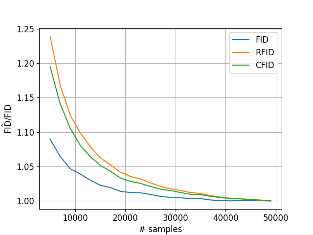
In the last experiment, we explore the sample complexity of CFID in practice. Following [27] we examine the dependence of the estimated values of RFID and CFID on the number of samples. Figure 6 shows the estimated values of the FID, RFID and CFID as a function of the number of samples, normalized on the values that were estimated using the entire test data (50k samples). We use the Pix2Pix model on the rotation task. As expected, the results show that all the metrics behave similarly. As noted in [27] for FID, all the metrics overestimate their population values. CFID and RFID both require more samples than FID, and CFID is a bit more efficient.
VI Discussion
In this paper, we considered conditional versions of the popular Wasserstein and Frechet distances. We introduced novel metrics and addressed their use in evaluating conditional generative models. In these settings, we showed that the conditional metrics outperform both the classical MSE metric and their corresponding unconditional metrics. In particular, a good conditional score signals that the model succeeded in its two tasks: generating realistic outputs that correspond to the correct input; and generating a diverse set of samples that fully capture the underlying output distribution.
There are many directions for future work on conditional metrics. Even within the Gaussian framework, stronger FID metrics can allow more expressive models, e.g. non-constant conditional covariances that depend on the inputs. For more realistic measures, non-Gaussian distributions should be considered as in [4, 10]. Theory can focus on sample complexity analysis of the different metrics and its dependence on the different parameters and embeddings.
References
- [1] Amjad Almahairi, Sai Rajeshwar, Alessandro Sordoni, Philip Bachman, and Aaron Courville. Augmented cyclegan: Learning many-to-many mappings from unpaired data. In International Conference on Machine Learning, pages 195–204. PMLR, 2018.
- [2] Hamed Alqahtani, Manolya Kavakli-Thorne, Gulshan Kumar, and Ferozepur SBSSTC. An analysis of evaluation metrics of GANs. In International Conference on Information Technology and Applications (ICITA), 2019.
- [3] Karim Armanious, Chenming Jiang, Sherif Abdulatif, Thomas Küstner, Sergios Gatidis, and Bin Yang. Unsupervised medical image translation using cycle-medGAN. In 2019 27th European Signal Processing Conference (EUSIPCO), pages 1–5. IEEE, 2019.
- [4] Akbar Assa and Konstantinos N Plataniotis. Wasserstein-distance-based gaussian mixture reduction. IEEE Signal Processing Letters, 25(10):1465–1469, 2018.
- [5] Yaniv Benny, Tomer Galanti, Sagie Benaim, and Lior Wolf. Evaluation metrics for conditional image generation. International Journal of Computer Vision, 129(5):1712–1731, 2021.
- [6] Mathilde Caron, Ishan Misra, Julien Mairal, Priya Goyal, Piotr Bojanowski, and Armand Joulin. Unsupervised learning of visual features by contrasting cluster assignments. arXiv preprint arXiv:2006.09882, 2020.
- [7] Jen-Tzung Chien and Chun-Lin Kuo. Variational bayesian GAN. In 2019 27th European Signal Processing Conference (EUSIPCO), pages 1–5. IEEE, 2019.
- [8] Min Jin Chong and David Forsyth. Effectively unbiased fid and inception score and where to find them. In Proceedings of the IEEE/CVF conference on computer vision and pattern recognition, pages 6070–6079, 2020.
- [9] Terrance DeVries, Adriana Romero, Luis Pineda, Graham W Taylor, and Michal Drozdzal. On the evaluation of conditional GANs. arXiv preprint arXiv:1907.08175, 2019.
- [10] P Dimitrakopoulos, G Sfikas, and Christophoros Nikou. Wind: Wasserstein inception distance for evaluating generative adversarial network performance. In ICASSP 2020-2020 IEEE International Conference on Acoustics, Speech and Signal Processing (ICASSP), pages 3182–3186. IEEE, 2020.
- [11] Xin Ding, Z Jane Wang, and William J Welch. Subsampling generative adversarial networks: Density ratio estimation in feature space with softplus loss. IEEE Transactions on Signal Processing, 68:1910–1922, 2020.
- [12] Ian J Goodfellow, Jean Pouget-Abadie, Mehdi Mirza, Bing Xu, David Warde-Farley, Sherjil Ozair, Aaron Courville, and Yoshua Bengio. Generative adversarial networks. arXiv preprint arXiv:1406.2661, 2014.
- [13] Martin Heusel, Hubert Ramsauer, Thomas Unterthiner, Bernhard Nessler, and Sepp Hochreiter. GANs trained by a two time-scale update rule converge to a local nash equilibrium. arXiv preprint arXiv:1706.08500, 2017.
- [14] Xun Huang, Ming-Yu Liu, Serge Belongie, and Jan Kautz. Multimodal unsupervised image-to-image translation. In Proceedings of the European conference on computer vision (ECCV), pages 172–189, 2018.
- [15] Xun Huang, Ming-Yu Liu, Serge Belongie, and Jan Kautz. Multimodal unsupervised image-to-image translation. In ECCV, 2018.
- [16] Phillip Isola, Jun-Yan Zhu, Tinghui Zhou, and Alexei A Efros. Image-to-image translation with conditional adversarial networks. In Proceedings of the IEEE conference on computer vision and pattern recognition, pages 1125–1134, 2017.
- [17] Steven M Kay. Fundamentals of statistical signal processing. Prentice Hall PTR, 1993.
- [18] Christian Ledig, Lucas Theis, Ferenc Huszár, Jose Caballero, Andrew Cunningham, Alejandro Acosta, Andrew Aitken, Alykhan Tejani, Johannes Totz, Zehan Wang, et al. Photo-realistic single image super-resolution using a generative adversarial network. In Proceedings of the IEEE conference on computer vision and pattern recognition, pages 4681–4690, 2017.
- [19] Jiguo Li, Xinfeng Zhang, Chuanmin Jia, Jizheng Xu, Li Zhang, Yue Wang, Siwei Ma, and Wen Gao. Direct speech-to-image translation. IEEE Journal of Selected Topics in Signal Processing, 14(3):517–529, 2020.
- [20] Ming-Yu Liu, Thomas Breuel, and Jan Kautz. Unsupervised image-to-image translation networks. In Advances in neural information processing systems, pages 700–708, 2017.
- [21] Shaohui Liu, Yi Wei, Jiwen Lu, and Jie Zhou. An improved evaluation framework for generative adversarial networks. arXiv preprint arXiv:1803.07474, 2018.
- [22] Ziwei Liu, Ping Luo, XiaoGANg Wang, and Xiaoou Tang. Deep learning face attributes in the wild. In Proceedings of the IEEE international conference on computer vision, pages 3730–3738, 2015.
- [23] Mario Lucic, Karol Kurach, Marcin Michalski, Sylvain Gelly, and Olivier Bousquet. Are GANs created equal? a large-scale study. arXiv preprint arXiv:1711.10337, 2017.
- [24] Luke Metz, Ben Poole, David Pfau, and Jascha Sohl-Dickstein. Unrolled generative adversarial networks. arXiv preprint arXiv:1611.02163, 2016.
- [25] Mehdi Mirza and Simon Osindero. Conditional generative adversarial nets. arXiv preprint arXiv:1411.1784, 2014.
- [26] Takeru Miyato and Masanori Koyama. cGANs with projection discriminator. In International Conference on Learning Representations, 2018.
- [27] Stanislav Morozov, Andrey Voynov, and Artem Babenko. On self-supervised image representations for gan evaluation. In International Conference on Learning Representations, 2020.
- [28] Naila Murray. PfaGAN: An aesthetics-conditional GAN for generating photographic fine art. In Proceedings of the IEEE/CVF International Conference on Computer Vision Workshops, pages 0–0, 2019.
- [29] Kristina Preuer, Philipp Renz, Thomas Unterthiner, Sepp Hochreiter, and Gunter Klambauer. Fréchet chemnet distance: a metric for generative models for molecules in drug discovery. Journal of chemical information and modeling, 58(9):1736–1741, 2018.
- [30] Suman Ravuri and Oriol Vinyals. Classification accuracy score for conditional generative models. arXiv preprint arXiv:1905.10887, 2019.
- [31] Eitan Richardson and Yair Weiss. The surprising effectiveness of linear unsupervised image-to-image translation. arXiv preprint arXiv:2007.12568, 2020.
- [32] Yossi Rubner, Carlo Tomasi, and Leonidas J Guibas. The earth mover’s distance as a metric for image retrieval. International journal of computer vision, 40(2):99–121, 2000.
- [33] Tim Salimans, Ian Goodfellow, Wojciech Zaremba, Vicki Cheung, Alec Radford, and Xi Chen. Improved techniques for training GANs. In Advances in neural information processing systems, pages 2234–2242, 2016.
- [34] Christian Szegedy, Vincent Vanhoucke, Sergey Ioffe, Jon Shlens, and Zbigniew Wojna. Rethinking the inception architecture for computer vision. In Proceedings of the IEEE conference on computer vision and pattern recognition, pages 2818–2826, 2016.
- [35] Thomas Unterthiner, Sjoerd van Steenkiste, Karol Kurach, Raphael Marinier, Marcin Michalski, and Sylvain Gelly. Towards accurate generative models of video: A new metric & challenges. arXiv preprint arXiv:1812.01717, 2018.
- [36] Cédric Villani. Optimal transport: old and new, volume 338. Springer Science & Business Media, 2008.
- [37] Zhou Wang, Alan C Bovik, Hamid R Sheikh, and Eero P Simoncelli. Image quality assessment: from error visibility to structural similarity. IEEE transactions on image processing, 13(4):600–612, 2004.
- [38] Sheng You, Ning You, and Minxue Pan. Pi-rec: Progressive image reconstruction network with edge and color domain. arXiv preprint arXiv:1903.10146, 2019.
- [39] Han Zhang, Tao Xu, Hongsheng Li, Shaoting Zhang, Xiaogang Wang, Xiaolei Huang, and Dimitris N Metaxas. Stackgan++: Realistic image synthesis with stacked generative adversarial networks. IEEE transactions on pattern analysis and machine intelligence, 41(8):1947–1962, 2018.
- [40] Richard Zhang, Phillip Isola, and Alexei A Efros. Colorful image colorization. In European conference on computer vision, pages 649–666. Springer, 2016.
- [41] Richard Zhang, Phillip Isola, Alexei A Efros, Eli Shechtman, and Oliver Wang. The unreasonable effectiveness of deep features as a perceptual metric. In Proceedings of the IEEE conference on computer vision and pattern recognition, pages 586–595, 2018.
- [42] Sharon Zhou, Mitchell L Gordon, Ranjay Krishna, Austin Narcomey, Li Fei-Fei, and Michael S Bernstein. Hype: A benchmark for human eye perceptual evaluation of generative models. arXiv preprint arXiv:1904.01121, 2019.
- [43] Jun-Yan Zhu, Taesung Park, Phillip Isola, and Alexei A Efros. Unpaired image-to-image translation using cycle-consistent adversarial networks. In Proceedings of the IEEE international conference on computer vision, pages 2223–2232, 2017.
- [44] Jun-Yan Zhu, Taesung Park, Phillip Isola, and Alexei A Efros. Unpaired image-to-image translation using cycle-consistent adversarial networkss. In Computer Vision (ICCV), 2017 IEEE International Conference on, 2017.
- [45] Jun-Yan Zhu, Richard Zhang, Deepak Pathak, Trevor Darrell, Alexei A Efros, Oliver Wang, and Eli Shechtman. Toward multimodal image-to-image translation. In Advances in Neural Information Processing Systems, 2017.
-A Proof of Lemma 2
This proof is quite technical and straight forward. We begin with the means: =
| (28) |
For the term
| (29) |
For the term
| (30) |
For the term
| (31) |
Thus
| (32) |
Now back to CFID, we conclude that:
| (33) | ||||
-B
Proof of Lemma 3
For convenience, we begin by recalling the definitions of the different distances:
| (34) |
| (35) |
| (36) |
| (37) |
| (38) |
Part 1: We begin by proving
CWD involves an infinite number of optimization problems parameterized by . We denote the optimal solution to CWD by . We then define
| (39) |
We prove the inequality by showing that (39) is feasible for RWD3 and yields the same objective. For this purpose, note that it is a legitimate distribution
| (40) |
and feasible since
| (41) |
| (42) |
Finally, it is easy to see that it gives the same objective value as CWD for:
| (43) |
| (44) |
Actually, the inequality is tight and . To prove this, we will show the other direction:
| (45) |
We denote the optimal solution to by . We then define
| (46) |
We prove the inequality by showing that (46) is feasible for CWD and yields the same objective. For this purpose, note that it is legitimate distribution for all :
| (47) |
Because is a valid solution for RWD3, thus:
| (48) |
That is, (46) is a legitimate distribution for all . Now we show that it also a valid solution:
| (49) |
| (50) |
Finally it yields the same objective value as RWD3 (as shown in (43)).
Part 2: Next, we continue to prove
RWD3 and RWD are very similar. The only difference is that RWD3 minimizes over , whereas RWD minimizes over . To prove the inequality, we denote the optimal solution to RWD3 by and claim that
| (51) |
is feasible for RWD and yields the same objective. Indeed, the delta function ensures that for any function . Therefore:
| (52) |
| (53) |
| (54) |
as required.
Part 3: Finally, it remains to show that
| (55) |
For this purpose, note that
Thus, we can omit the squared norm associated with . Next, we denote the optimal solution to RWD by and define
| (58) |
This bivariate distribution is feasible for MWD and yields the same objective value as required.
Now we prove the second part of the lemma, that is:
| (59) |
We prove the inequality is tight if we replace RWD by RWDα with . For this purpose, note that:
| (60) |
For unbounded , RWDα is finite only if . Thus, the optimal solution satisfies
| (61) |
where is the delta of Dirac. This is exactly the definition of RWD3 which is identical to CWD.
For , the joint distributions and are reduced to the marginal distributions and and the objective is reduced to . Thus, .
Finally, we show that is invariant to . Note that:
| (62) |
Changing variables in the integral over : gives the same value as the original CWD.