A Deep Deterministic Policy Gradient-based Strategy for Stocks Portfolio Management
Abstract
With the improvement of computer performance and the development of GPU-accelerated technology, trading with machine learning algorithms has attracted the attention of many researchers and practitioners. In this research, we propose a novel portfolio management strategy based on the framework of Deep Deterministic Policy Gradient, a policy-based reinforcement learning framework, and compare its performance to that of other trading strategies. In our framework, two Long Short-Term Memory neural networks and two fully connected neural networks are constructed. We also investigate the performance of our strategy with and without transaction costs. Experimentally, we choose eight US stocks consisting of four low-volatility stocks and four high-volatility stocks. We compare the compound annual return rate of our strategy against seven other strategies, e.g., Uniform Buy and Hold, Exponential Gradient and Universal Portfolios. In our case, the compound annual return rate is 14.12%, outperforming all other strategies. Furthermore, in terms of Sharpe Ratio (0.5988), our strategy is nearly 33% higher than that of the second-best performing strategy.
Index Terms:
Reinforcement Learning, Deep Learning, Portfolio ManagementI Introduction
Portfolio management is generally defined as the process of allocating assets such as stocks, futures and options by constructing an internal representation (model) of the markets[1]. Based on existing theories, many timing strategies, stock-picking strategies, statistic arbitrage and portfolio management strategies are proposed in the last decades. For example, Dzitkowski and Kozicki employed Long Short-Term Memory (LSTM) in High Frequency Trading[2]; Mehtab, Sen and Dutta analyzed the sentiments in social media and utilized the sentiment-related information based on self-organizing fuzzy neural networks (SOFNN) to predict stock price[3]. Such supervised-learning algorithms rely on historical information, e.g., price information, calculated indices, non-financial information and other information to predict future price movements. Unfortunately, given the efficient market hypothesis and non-stationarity property in the price time series, it is seemingly impossible to truly make price predictions timely and accurately. Furthermore, price prediction does not translate directly into actual market action. In addition to the prediction of price movement, rational judgment is also required to implement portfolio strategy.
Recently, many studies on the use of reinforcement learning have drawn much attention of research not only because they no longer need to predict price, but due to their superior performance in Board Games, Go, and Video Games[4], which mimic the environment of financial market to some extent. Gao et al.[5] [24] discretized the action space which is defined as the weight of portfolio wealth in different stocks, and combined the Convolutional Neural Network (CNN) with dueling Q-net (DQN) to obtain the optimal actions. However, finite action space models might result in local optimum or no optimum at all, as they are limited by the number of action combinations. Besides, Gao et al.’s strategy model[5] [24] and many other traditional strategies such as Exponential Gradient (EG)[20] and Online Moving Average Reversion (OLMAR)[21] dismiss transaction cost. Apart from the above limitations, some strategies are simply tested in a short period of time, e.g., spanning one or two years, which makes it difficult to experience different market phases.
In this paper, instead of discretizing the continuous action space into finite action space, we use a Deep Deterministic Policy Gradient (DDPG)[4] framework specifically designed for multi-asset trading strategy in continuous action space. This framework allows the DDPG agent to receive the market states and then optimize trading policies (actions), which are the portfolio wealth allocations in different time steps. The framework will output the optimized trading policies (actions) for each time step, which we will subsequently use to calculate the returns and other performance metrics to evaluate our DDPG-based strategy.
The motivation of our work is two-fold. First, the need of applying reinforcement learning model in continuous action space in portfolio management inspires us to apply the DDPG framework. Second, different from previous work which dismisses transaction cost[5] [17] [21] [19], we want to explore the impact of transaction cost on our strategy.
The novelty of our work is as follows: Unlike other DDPG-based models where CNN are employed as both critics and actors network[5][10], we propose a new framework, which consists of two LSTM networks working as critic and target-critic network respectively, as well as two fully connected (FC) networks working as actor and target-actor.
The key contribution of our research is that we compare our DDPG-based strategy’s performance under the conditions with and without transaction cost, and discover a counterintuitive result that the strategy with transaction cost is more robust and profitable than that without transaction cost, we also provide a plausible explanation for this phenomenon in our experiment. Furthermore, we assess the efficiency of our strategy against seven other traditional strategies using the same dataset, and find their returns are neither as stable nor as high as our DDPG strategy. The compound annual return rate of our DDPG strategy (14.12%) is at least twice as much as other traditional strategies. In terms of Sharpe Ratio (SR), our DDPG strategy (0.5988) is nearly 33% higher than that of the second best strategy (0.3679).
The organization of the rest of this paper is as follows. Section II describes the dataset we use. Section III provides a mathematical treatment to our problem, and also gives a brief introduction to our DDPG strategy in comparison to other traditional RL methods. Section IV proposes some basic assumptions used in our research, Section V presents a detailed description of our strategy. Section VI contains the results as well as the analysis of our strategy. Finally in Section VII, conclusions of the research and future research directions are given.
II Dataset and Features
The stock data comes from Yahoo Finance including eight US stocks ranging from July 1999 to July 2020. Notably, the data includes the 2008 market crash as well as 2020 Covid-19 market crisis in order to train and test our model with real world fluctuations. We choose four stocks with low volatility measured by and four stocks with high volatility to formulate our portfolio. Four high volatility stocks are: , , , [7](see Figure 1(a)); four low volatility stocks are: , , , [8](see Figure 1(b)).
For data pre-processing, we calculate the Relative Strength Index of two-day time period (RSI2), daily simple return rate and logarithm daily return rate for each stock. Furthermore, we directly drop off the empty values since the price information for some stocks are not available every day, but such situation is rare, which means directly omitting empty values will not significantly influence our result.


(a)Adjusted Prices of High Volatility Stocks; (b)Adjusted Prices of Low Volatility Stocks
III Problem Statement
Portfolio management is the action of continuous reallocation of a capital into a number of financial assets[23]. In practice, the investors modify the weight of portfolio in different assets at each trade period. In this work, we set the trade period as one day. We shall first provide some mathematical notations:
- •
: The number of assets, here we have
- •
[1]: Portfolio vector, its -th component represents the ratio of the total budget invested to the -th asset at time , such that
- •
: The adjusted closing price of stock at time
- •
: The RSI of two-day time period of stock at time
- •
: The shares holding of stock at time
where means the largest integer less or equal than
- •
: Portfolio Value at time
- •
: Cash owned at time
- •
: State at time , a tuple consisting of , where and , thus
- •
: Reward at time , defined as:
- •
: Action taken at time , we treat it as the the ratio of total budget of each asset, i.e.
- •
: The probability that if .
- •
: The value of taking action in state under a policy
where is called discounting factor
Traditionally, the reinforcement learning problem is a straightforward framing of the problem of learning from interaction between agent and environment to achieve a goal. The learner and decision-maker is called the agent, while the environment is the outside thing it interacts with. These interact continuously, i.e., the agent chooses actions, and the environment responds to the actions and return rewards that the agent seeks to maximize overtime. To achieve this, the agent needs to modify its action following policy, a mapping from states to probabilities of selecting each possible action[9].
If both the action space and state space are not large, rendering a possibility to record the value of all combination of states and actions , the agent can determine its optimal action by looking up the value from -table, i.e.

In our experiment, however, the state space is of 42-dimension, and each entry of one state is a continuous real number, and so as the action space. Therefore, it is neither feasible nor reasonable to use table-lookup method to obtain the optimal policy. We shall use DDPG as our basic model because it does not have special requirements for state space and action space, which means it can solve either finite or infinite space problems.
IV Assumptions
- •
Assumption 1: The liquidity of all market assets is high enough that, each trade can be executed immediately at the orderd price, i.e. zero slippage.
- •
Assumption 2: The action of agent will not affect the market.
- •
Assumption 3: A small transaction cost per transaction ($0.001) was used to encapsulate the various trading fees[6], and no other commisions.
- •
Assumption 4: The portfolio keeps unchanged during the period from the end of previous trading day and the beginning of next trading day.
- •
Assumption 5: No other assets are chosen besides the selected stocks.
- •
Assumption 6: The volume of each stock is large enough, so the model can buy or sell every stock at any trading day.
V Methods
V-A From Actor-Critics Methods to DDPG
Actor–critic methods[4] are temporal-difference (TD) methods with a separate memory structure to explicitly represent the policy without depending on the value function. The policy structure is known as the actor, since it is used to select actions given the input state. The estimated value function is known as the critic as it evaluates the action value made by the actor. The critic learns about and critique the policy being adopted by the actor. The critique takes the form of a TD error[9]:
where is the current value function implemented by the critic.

Typically, the critic is a function with state as input and an evaluation value as output. After each action is selected, the critic evaluates the new state to see if things turn out to be better or worse than expected. Similarly, following the feedback from critic, the actor learns how valuable its action is, and tends to choose the optimal action.
Essentially, both the critic and actor are function approximators, and therefore we can use neural network to construct them. The DDPG algorithm (Figure 4) can generate deterministic actions directly from the policy of actor without sampling according to the probability distribution of action, so it is called deterministic policy. In the learning phase, a noise function is added to the deterministic action to realize the small-scale exploration near such deterministic action[11]. In addition, the algorithm also backups a set of parameters for actor and critical network respectively to calculate the expectation of action value, so as to improve the guidance level of critics[4]. The networks using the backup parameters are called the target networks. The purpose of such two sets parameter design (backup parameters and real-time updating parameters) is to reduce the non-convergence caused by the approximated data[9].

The specific application scenarios of these four networks are as follows:
- •
Actor Network: According to the current state , generating specific action of exploring or not exploring.
- •
Target-Actor Network: Based on the follow-up state given by the environment, a new action is generated.
- •
Critic Network: Computing state-action value
- •
Target-Critic Network: Given subsequent state-action pair , calculating to compute expected , i.e.,
V-B Data Processing
Since the inputs of critic network and target-critic network are state and action , we concatenate these two vectors to form a new vector .
V-C Network Frameworks
For the critic network and target-critic network, we choose an LSTM network (figure 5) with 3 hidden layers for implementation. The LSTM is a promising choice to handle with time-series as it is effective in solving the problems regarding gradient vanish and gradient explosion.

The input dimension is since our mini-batch size is . The hidden size (node number) of the first layer and second layer are respectively. We also set hyperparameter “dropout” to 0.35. Following the first two LSTM layers, we construct a fully connnected layer with hidden size , and finally an output layer showing value(Figure 6).

To evalute the critic network, we use Huber-Loss with :

For actor network (Figure 8), we use fully connected (FC) network layout. The input is the state variable of 42-dimensioned. The size of three hidden layers are respectively, with function as activation. The output is an 8-dimensioned action vector with each entry . Thus we use function to project the raw output to interval . The loss function of actor network[4] is as follows:
where is the output of actor network, is the mini-batch size, is the output of critic network.

V-D Tradeoff between Exploitation and Exploration
We use -greedy algorithm to provide a balance between exploitation and exploration. For each learning, the program generates a random number between 0 and 1, saying , if , we exploit, and if , we explore using Ornstein Uhlenbeck Action Noise (OU noise) algorithm[13] instead of Gaussian Noise, as OU noise is autocorrelated while Gaussian Noise are time-independent (Figure 9). In particular, we set a batch of stratified in our experiment:
We firstly denote as the total state number our model has experienced at time .
We also set the soft update hyperparameter to be 0.09.

V-E Performance Metrics
Three different metrics have been used to evaluate the performance of trading strategies. The first is Compound Annual Return Rate (CARR), which is defined as:
where:
- •
: The portfolio wealth at the last test day.
- •
: The portfolio wealth at the begining test day.
- •
: Number of years
The second metric is Sharpe Ratio (SR) which mainly represents the risk adjusted return of strategies. [15]:
where
and represents the rate of return of risk-free asset. We set in our experiment.
The third metric is the Maximum Drawdown (MDD), which we use to assess the risk resistance of an investment strategy completely[16].
where and represent different time steps.
This metric denotes the maximum portfolio value loss from a peak to bottom.
VI Result and Analysis
VI-A Settings
We set initial money to be 1,000,000, and the trading frequency is daily. In other words, we reallocate our portfolio everyday. We also choose the data from July 1999 to July 2016 as training set, and backtest our strategy in the whole dataset from July 1999 to July 2020.
For a more intuitive comparison, we choose a benchmark strategy: At the first test day, we allocate the same amount of money to each stock, i.e. , then we hold these stocks shares until the end test day.
VI-B Cost-Free DDPG Strategy
We first give the result of the Cost-free DDPG strategy (Figure 10), in which we omit the transaction cost. From this figure, we observe that the performance of the Cost-free DDPG strategy from 1999 to the end of 2008 does not exceed that of the benchmark strategy. The performance of the two strategies is almost identical in this time period. However, starting from 2009, the Cost-free DDPG strategy performs significantly better than the benchmark strategy, even though it experiences larger drawdowns in 2015, 2018 and 2020. To some extent, the Cost-free DDPG strategy is an amplification of the benchmark strategy, both on return and loss. The Cost-free strategy’s Compound Annual Return Rate (CARR) is 11.78%, Sharpe Ratio (SR) is 0.4781, Maximum Drawdown (MDD) is 56.67%.

VI-C Cost DDPG Strategy
The return curve of the Cost DDPG strategy is given in Figure 11, where we take into account of the transaction cost of $0.001 per share for each transaction. Also, the profit distribution histogram is presented (Figure 12).

Compared to the benchmark strategy, the return of Cost DDPG strategy outperforms that of benchmark from 2001, which is earlier than the Cost-free DDPG strategy. After 2001, the return of Cost DDPG strategy start to steadily increase until 2008, with the arrival of the global financial crisis. Both benchmark strategy and Cost DDPG strategy experience a pronounced drawdown, while the drawdown of Cost DDPG strategy is less than that of the benchmark. Since 2008, Cost DDPG strategy’s return begins to rise again. If we particularly focus on the time period after July 2016, the return of the Cost DDPG strategy continuously increases until the beginning of 2020, as the Covid-19 epidemic deals a huge blow to the global market. Finally, the Cost DDPG strategy’s Compound Annual Return Rate (CARR) is 14.12%, Sharpe Ratio (SR) is 0.5988, Maximum Drawdown (MDD) is 49.13%.

VI-D Comparison Between Cost Strategy and Cost-free Strategy
Both Cost-Free strategy and Cost strategy performed similarly in the first two years, so does the benchmark strategy. It is possible to explain this as both strategies underfitted at the initial stage since the training data is not sufficient enough. Starting from 2001, all three strategies increase steadily until 2008, when all strategies experience a significant drawdown, but the Cost DDPG strategy is the most robust during this period, with its drawdown being the smallest among the three. Subsequently, the returns of all three strategies rebound to varying degrees, but the returns of both the Cost-free DDPG strategy and the benchmark strategy remain volatile after 2011. When we specifically focus on time period after 2016, both Cost-free and Cost DDPG strategies make profits during this period, despite their returns declining sharply in 2020 due to Covid-19.
One counterintuitive result is that the Cost DDPG strategy performs better than the Cost-Free DDPG strategy in our experiment. We should provide a plausible explanation here: The transaction cost added in reward function could be treated as a small constant penalty term, which will encourage our model to choose cautious actions, i.e. the actions making profits not only without transaction cost, but also with transaction cost. Moreover, a small amount of transaction costs can also make the strategy profitable without expending too much on transaction fees.
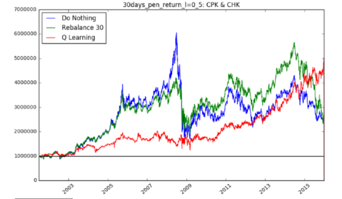
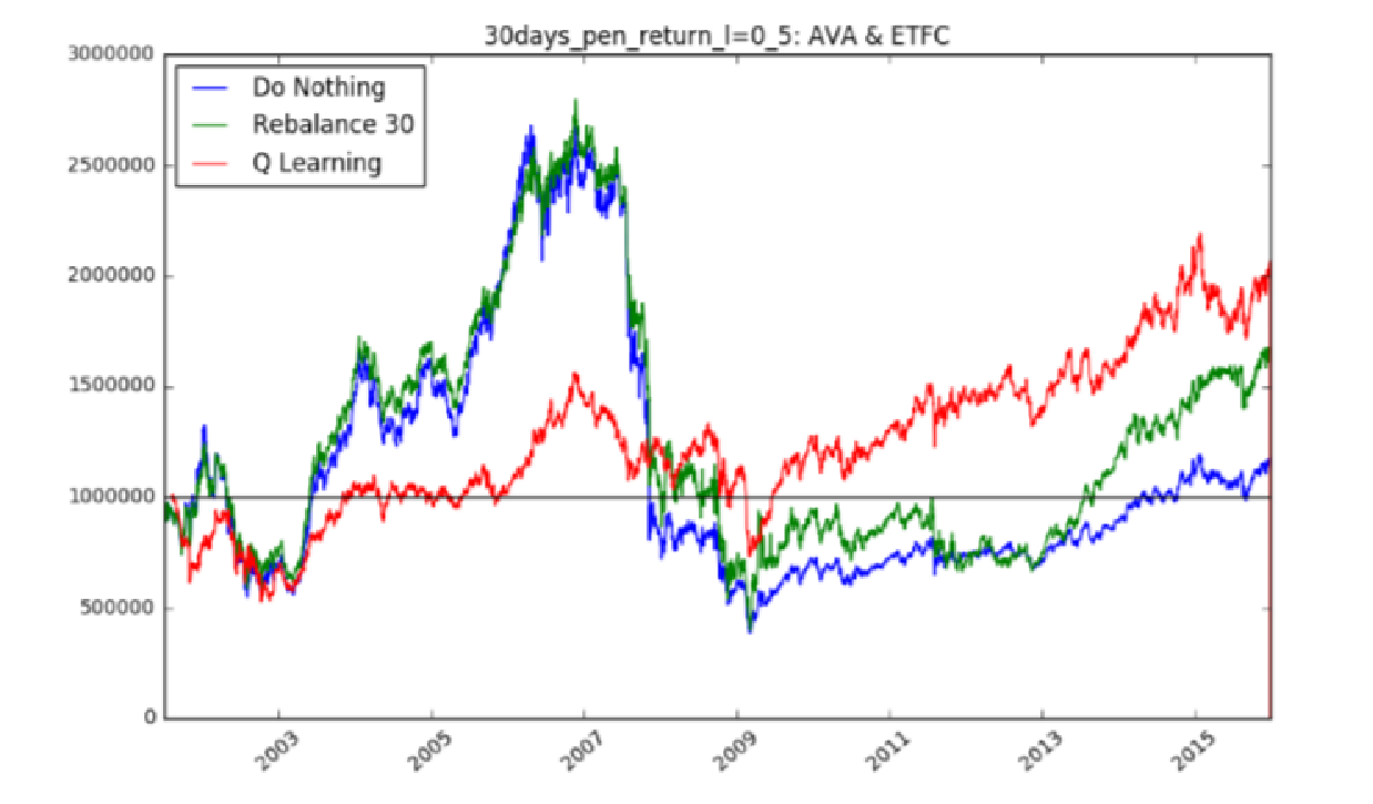
Jin and El-Saawy[6]’s work indicates that a penalty term added in reward might make the strategy more robust and profitable. This partly validates our explanation on why Cost DDPG strategy outperforms the Cost-free DDPG strategy. They modify the portfolio reward to include a penalty for volatility:
where is the portfolio value at time , is the penalty factor, and is the modified portfolio value at time , is the variance. They test their Deep Q-Learning strategy (DQN) in different portfolio, and found out the penalized strategy are more stable even in different markets. Figure 13 shows their DQN strategy performance while choosing CPK and CHK as trading stocks, and Figure 14 presents the result in AVA and ETFC.
VI-E Strategy Comparison
We compare our cost DDPG-based strategy with several traditional strategies as below:
- •
Aniticor (ANTICOR) [17]
- •
The Uniform Buy and Hold (BAH), a portfolio management approach simply equally spreading the total wealth into the selected assets and holding them without making any purchases or selling until the end. This is our benchmark strategy in previous graphs.[18]
- •
Uniform Constant Rebalanced Portfolios (CRP) [19]
- •
Exponential Gradient (EG) [20]
- •
Online Moving Average Reversion (OLMAR) [21]
- •
Passive Aggressive Mean Reversion (PAMR) [22]
- •
Universal Portfolios (UP) [19]
All the above strategies are tested with the same transaction cost as our cost DDPG-based strategy. Figure 15 illustrates the accumulative return over the investment horizon of the test period.

| CARR | SR | MDD | |
| Anticor | 7.94% | 0.3679 | 0.8117 |
| BAH | 4.37% | 0.2711 | 0.6423 |
| CRP | 5.77% | 0.3141 | 0.6428 |
| EG | 5.39% | 0.3027 | 0.6415 |
| OLMAR | -4.06% | 0.2331 | 0.9780 |
| PAMR | 6.09% | 0.3595 | 0.9501 |
| UP | 4.95% | 0.2892 | 0.6394 |
| DDPG | % |
Overall, our cost DDPG strategy outperforms other strategies for the majority of the test trading period, though the advantage is not obvious at the beginning. The difference between cost DDPG strategy and others becomes obvious especially in the last few trading periods. Despite the excellent performance of the PAMR and OLMAR strategies from 2009 to 2010, their ultimate performance are worse than that of cost DDPG strategy due to the sharp decline after 2010. Both MDD and SR suggest the instability of these two strategies, which makes them vulnerable to the market full of risk. The performance metrics table(Table 1) indicates that the numerical results of cost DDPG strategy are the best among other strategies in profitability and stability aspects. In terms of CARR, the result of the DDPG strategy (14.12%) is almost twice than that of the second largest benchmarks Anticor (7.94%) over the test trading period. As for the risk measure, the cost DDPG strategy still has the best performance by holding the minimum MDD (0.4913), comparing with the UP strategy (0.6394) which is the second lowest. In terms of SR, cost DDPG strategy (0.5988) is nearly 33% larger than that of Anticor strategy (0.3679), which is the second largest.
In conclusion, the aforementioned results demonstrate the outstanding and stable profitability of DDPG strategy in comparison with other traditional strategies.
VII Conclusions and Future Work
VII-A Conclusions
In this paper, we propose a novel pattern of DDPG reinforcement learning framework, including the LSTM critic network and the Fully Connected actor network. This DDPG strategy makes profits in our selected portfolio set — 4 low volatility U.S stocks and 4 high volatility U.S stocks. Moreover, we use Compound Annual Return Rate, Sharpe Ratio, and Maximum Drawdown as performance metrics. In our experiment, the Cost DDPG strategy outperforms seven other traditional strategies in all three performance metrics. We also compare the performance of our DDPG strategy with and without transaction cost, and provide a plausible explanation to the result that DDPG strategy with transaction cost is more profitable and more robust than the Cost-free strategy.
Our strategy still has a number of drawbacks. First, we assume that there is no transaction slippage (Assumption 1), which is unrealistic in real market. Random transaction slippage happening might result in unexpected results in strategy reward. Second, we assume that each stock is available on any trading day (Assumption 6). Nevertheless, the stock might not be available sometimes, which will influence the return as well.
VII-B Future Work
For future work, we shall look into an improved DDPG strategy with transaction slippage in order to simulate the real market. The slippage might cause the strategy not to trade at the expected price, and then lead to the decline of profit. To solve this, we will try to modify the reward function so that the loss caused by slippage will be considered. Moreover, we will consider the situation that some stocks are not avaible in particular days. One possible solution to this problem is to expand our portfolio divisions, which will reduce the impact of non-tradable stocks on final return. Futhermore, our improved strategy will try to include short transactions by modifying the action space.
References
- [1] A. Filos,“Reinforcement Learning for Portfolio Management,” , 2019, arXiv:1909.09571v1.
- [2] K. Dzitkowski and T. Kozicki, “High Frequency Trading Price Prediction using LSTM Recursive Neural Networks,” 2015.
- [3] S. Mehtab, J. Sen and A. Dutta, “Stock Price Prediction Using Machine Learning and LSTM-Based Deep Learning Models,” , 2009, arXiv:2009.10819.
- [4] D. Silver, G. Lever, N. Heess, T. Degris, D. Wierstra, and Martin Riedmiller, “Deterministic Policy Gradient Algorithms,” , pages 387–395, 2014.
- [5] Z. Gao, Y. Gao, Y. Hu, Z. Jiang and J. Su, “Application of Deep Q-Network in Portfolio Management,” 2020 5th IEEE International Conference on Big Data Analytics (ICBDA), Xiamen, China, pp. 268-275, 2020
- [6] O. Jin and H. El-Saawy, “Portfolio Management using Reinforcement Learning,” Stanford University, 2016
- [7]
Market Watch(2020, December 20)[Online]. Available: https://www.marketwatch.com/investing/fund/sphb/holdings?
mod=mw_quote_tab - [8] Yahoo Finance(2020, December 20)[Online]. Available: https://finance.yahoo.com/news/navigate-market-volatility-5-low-140802735
- [9] R.S. Sutton and A.G. Barto, Reinforcement Learning: An Introduction, MA: MIT Press, 2012
- [10] Z. Liang, H. Chen, J. Zhu, K. Jiang and Y. Li, “Adversarial Deep Reinforcement Learning in Portfolio Management ,” , 2018, arXiv:1808.09940v3.
- [11] T.P. Lillicrap, J.J. Hunt, A. Pritzel, N. Heess, T. Erez, Y. Tassa, D. Silver and D. Wierstra, “Continuous Control With Deep Reinforcement Learning,” , 2019, arXiv:1509.02971v6.
- [12] R.C. Staudemeyer and E.R. Morris, “Understanding LSTM – a tutorial into Long Short-Term Memory Recurrent Neural Networks,” , 2019, arXiv:1909.09586v1.
- [13] G.E. Uhlenbeck and L.S. Ornstein, “On the theory of the brownian motion,” , 36(5): 823, 1930.
- [14] Y. Deng, F. Bao, Y. Kong, Z. Ren, and Q. Dai, “Deep direct reinforcement learning for financial signal representation and trading,” IEEE transactions on neural networks and learning systems, vol. 28, no. 3, pp. 653–664, 2017
- [15] W. F. Sharp, “The sharpe ratio,” The journal of portfolio management, vol. 21, no. 1, pp. 49-58, 1994, doi:10.3905/jpm.1994.409501.
- [16] M. Magon-Ismail and A. F. Atiya, “Maximum drawdown,” Risk Magazine, vol. 17, no. 10, pp. 99-102, 2004.
- [17] A. Borodin, R. El-Yaniv, and V. Gogan, “Can we learn to beat the best stock,” Journal of Artificial Intelligence Research, vol. 21, pp. 579, 2004.
- [18] B. Li and S. C. H. Hoi, “Online portfolio selection: A survey,” ACM Computing Surveys, vol.46, pp.35, 2014.
- [19] T. M. Cover, “Universal portfolios,” Mathematical finance. An International Journal of Mathematics, Statistics and Financial Economics, vol. 1, no. 1, pp. 1, 1991.
- [20] D. P. Helmbold, R. E. Schapire, Y. Singer, and M. K. Warmuth, “Online portfolio selection using multiplicative updates,” Mathematical Finance, vol. 8, no. 4, pp. 325–347, 1998.
- [21] B. Li, S. C. Hoi, D. Sahoo, and Z. Liu, “Moving average reversion strategy for on-line portfolio selection,” Artificial Intelligence, vol. 222, pp.104-123, 2015, doi:10.1016/j.artint.2015.01.006.
- [22] B. Li, P. Zhao, S. C. H. Hoi, and V. Gopalkrishnan, “PAMR: Passive Aggressive Mean Reversion Strategy for Portfolio Selection,” Machine Learning, vol. 87, no. 2, pp.221, 2012.
- [23] Z. Jiang, D. Xu, and J. Liang, “A deep reinforcement learning framework for the financial portfolio management problem,” arXiv, 2017, arXiv:1706.10059.
- [24] Y. Gao, Z. Gao, Y. Hu, S. Song, Z. Jiang, and J. Su, “A Framework of Hierarchical Deep Q-Network for Portfolio Management“. In Proceedings of the 13th International Conference on Agents and Artificial Intelligence - Volume 2: ICAART, ISBN 978-989-758-484-8, pages 132-140. DOI: 10.5220/0010233201320140, 2021