Expected Extinction Times of Epidemics with State-Dependent Infectiousness
Abstract
We model an epidemic where the per-person infectiousness in a network of geographic localities changes with the total number of active cases. This would happen as people adopt more stringent non-pharmaceutical precautions when the population has a larger number of active cases. We show that there exists a sharp threshold such that when the curing rate for the infection is above this threshold, the expected time for the epidemic to die out is logarithmic in the initial infection size, whereas when the curing rate is below this threshold, the expected time for epidemic extinction is infinite. We also show that when the per-person infectiousness goes to zero asymptotically as a function of the number of active cases, the expected extinction times all have the same asymptote independent of network structure. We make no mean-field assumption while deriving these results. Simulations on real-world network topologies bear out these results, while also demonstrating that if the per-person infectiousness is large when the epidemic size is small (i.e., the precautions are lax when the epidemic is small and only get stringent after the epidemic has become large), it might take a very long time for the epidemic to die out. We also provide some analytical insight into these observations.
Index Terms:
Epidemic modeling, network analysisI Introduction
Newly emerging infectious diseases that quickly spread across population centers in an increasingly interconnected world form a large portion of human infections [1]. These epidemics spread over contact networks and the characteristics of this spread have been widely studied [2, 3, 4, 5, 6, 7, 8]. In this work, we develop a state-dependent infectiousness model for the spread of epidemics over a network of population centers and analytically prove that the epidemic dynamics follow certain properties. Specifically, we characterize the expected time of epidemic extinction and show that it exhibits a threshold behavior where it is either logarithmic in the initial infection size or infinite depending on whether the curing rate is higher or lower than a threshold. We make no mean-field assumption while deriving this threshold. We believe our model captures important features of epidemic spreading not captured in prior literature, and our results advance the understanding of epidemic spread.
We model the epidemic as a Markov spreading process over a network whose nodes represent population centers such as cities or large communities, and the connections between them indicate the amount of contact between the population centers. New infections could either be due to interactions with people from neighboring population centers, or due to community spread within the population center. We model these two components of epidemic spread separately.
In a typical epidemic, especially in the early stages of newly emerging infections, vaccines and other pharmaceutical means to combat the disease are unlikely to be available. Further, in the early stages of the epidemic, the number of susceptible people in a typical population center is very large, and effectively infinite, until a large majority of the population has developed herd immunity. We capture these properties in a model where the number of infections in each population center can potentially grow without bound.
In cases where the infected population is a significant fraction of the total population, the epidemic would spread more slowly than what is predicted by our model. This is because for a given number of infected individuals, our model assumes that the susceptible population is larger than it actually is. So our model would over-estimate the effective rate at which the contagion spreads, and the number of (new) infections in our model stochastically dominates the actual number of infections. Thus, in those settings, the threshold obtained from our model would still hold for the quick-extinction case.
Whereas models at the person level [9, 10, 11, 12, 13] capture interactions between individual people and might help us predict the probability of a particular person getting infected, it is prohibitively expensive to collect information about all individuals in a city and compute over a network that treats each person as a distinct node. Population center-level models allow us to predict the epidemic trajectory over a much larger number of people at the level of countries or even the world.
Related work on metapopulation [14, 15, 16, 17] also develops population center-level models, but uses a mean field-type approximation, which assumes the existence of a (sharp) threshold and finds it. In contrast, sharp thresholds emerge in our work. Like [9, 10], we directly characterize the time it takes for epidemic extinction. But unlike [9, 10], where there is a gap between the conditions for a short- and long-lasting epidemic, we prove there is a sharp threshold for the curing rate which separates the conditions for short- and long-lasting epidemics.11 1 Note that the “mean field” described in [10] is over the network, not the infection probabilities. Note that our model is at the population center-level (compared to the person-level model in [9, 10]). Besides the work on metapopulation, other prior work which claim a sharp threshold between the two regimes [11, 18, 12, 13] have assumed it and employed a mean field-type approximation. Our analysis is significantly different from the analysis of the extinction time of the mean-field dynamics. The advantage of this stochastic-analysis framework is that it allows the possibility of obtaining tail bounds for the extinction time, whereas the existing mean-field models, in their current form, do not offer that scope. While we do not present tail bounds on extinction time in this work, in Sec. VI, we plot the confidence bounds on the extinction times obtained from simulations of the stochastic dynamics.
Another key aspect of our model is that the per-person infectiousness of the epidemic is a function of the number of active cases in the system. State-dependent infectiousness influences the epidemic trajectory as people tend to take more precautions [19, 20, 21] and governments tend to impose more restrictions on travel, gatherings, etc. [22, 19] as the number of active cases increases. Moreover, these changes in contact can be well-described using changes in the parameters of standard epidemiological compartment models [23]; models that incorporate these considerations may yield predictions that are significantly different from models that do not [24]. As explained in [25], modeling the effects of human behavior on epidemic spread is necessary for realistic models. Although time-dependent infectiousness has been studied empirically in [26], we analytically model infectiousness as a function of the number of active cases in the system, which provides a (tractable) theoretical basis to time-varying infectiousness. A person-level model for state-dependent infectiousness has been developed in [10], but as explained earlier, modeling the epidemic at the population center-level allows us to predict the epidemic trajectory over a much larger number of people. We prove the population center-level model has a sharp epidemic threshold for the extinction times, in contrast to the gap between the conditions for short- and long-lasting epidemics in [10]. Related to this are [12] and [13], which develop person-level models where individual people get alerted in the presence of infected neighbors and take more precautions or change their contacts.
Other related work on epidemic extinction time include [27] which estimates extinction time in SIR networks using simulations; [28] which calculates the extinction-time distribution in an aggregate non-network model; [29] which computes the mean extinction times for all possible configurations of small networks; [30, 31] which use the Wentzel-Kramers-Brillouin approximation; and [32] which characterizes the epidemic extinction times over a “mean” network formed from a given degree distribution.
To summarize, our main contribution is a sharp, analytical, and direct (not mean-field) characterization of the extinction time in a population center-level model with state-dependent infectiousness. This, to the best of our knowledge, is new.
The remainder of this paper is organized as follows. Sec. II describes our model. Under this model, Sec. III proves the existence of a sharp threshold: if the curing rate is greater than this threshold, the mean time for epidemic die-out starting from a state with a cumulative of infections is of order , and if the curing rate is below this threshold, the mean die-out time is infinite. Sec. IV generalizes the results to settings with asymmetric and weighted graphs. Then Sec. V proves that the asymptotic mean extinction time is (exactly) equal to independent of graph structure if the per-person infectiousness functions go to zero asymptotically. This would happen if the level of precautions people take to combat the epidemic keep getting more stringent with increasing numbers of active cases. Sec. VI provides simulation and computation results, and Sec. VII concludes.
II Model
Let there be a set of localities22 2 Note that “localities” can refer to population centers at various levels of demographic aggregation. They could represent countries, states, cities, or even neighborhoods within a city. Indeed, there can be marked differences in how people react to a contagion even within a single large urban area [33]. , and at each locality , the number of infected people at time is given by . We assume each locality has a large enough population that for our purposes, for all , the range of is the set of all non-negative integers. There is a graph across the localities, and when the localities and are connected. The adjacency matrix of is the matrix having if and otherwise. For ease of presentation, we first assume that the graph is symmetric: implies . We relax this assumption in Sec. IV. A connection between two localities means that infected people in one locality can infect susceptible people in the other locality. Further, we assume the graph is connected, i.e., for every , there exists a path between and in .
Let the total number of people infected at time be , i.e., . The rate of growth of the infection at locality at time consists of two components:
- 1.
the intra-locality growth rate due to interactions within the locality given by , and
- 2.
the between-locality growth rate, where the rate of growth due to for each is given by .
Here, and are positive real-valued functions of the total number of infections in the system, which give the rate of growth of the infection per infecting agent. We assume that these per-person infectiousness functions are bounded. Let their suprema be given by and . We also assume that the asymptotic limits for these functions exist as the total number of infections grows without bound: and . Let the curing rate for every infected agent be . This is independent of the graph , the level of precautions taken ( and ), or the number of infections at any node , and just depends on the nature of the infection. We show the model pictorially in Fig. 1.
For each , the above discussion implies the following rates for the infection:
| (1) |
Let us use the vector to denote the state of the system at time . The th element of is , the number of infections at node at time . Let denote the time it takes to go from a state to the all-zero state . Once the epidemic reaches the all-zero state, it is extinct, since one can only contract the infection from someone else,33 3 Note that this is true for many viral infections since the only host for these viruses are humans. However, this may not be the case for other infections. and if there are no infected individuals, the epidemic can never rebound later. The mean extinction time (also called the mean hitting time) starting from the state is given by .
III Sharp Threshold
In this section, we state our main result as Theorem 1.
Theorem 1.
Let and . Let denote the spectral radius of the adjacency matrix of the (symmetric) undirected graph . Let the system start in some state that has infections cumulatively, i.e., . If the graph is connected, then the following hold.
- (i)
If , then for some constant .
- (ii)
If , then .
Before we prove Theorem 1, let us first observe a property of the spectral radius, , of . Since we have assumed that is connected, the Perron-Frobenius theorem (see [34]) implies that every element of the eigenvector corresponding to is strictly positive, i.e., .
We prove Theorem 1 in two parts: (i) , and (ii) .
III-A Curing rate above the threshold
For proving part (i) of Theorem 1, the following claim, which follows from analyzing the time evolution of along the eigen-direction of , is useful.
Claim 1.
When and are constant, i.e., and for all , and , then for some where .
Proof:
Please see Appendix A. ∎
We are now ready to prove part (i) of Theorem 1.
Proof:
Since we have , , and , it follows from the definition of limit [35] that there is an such that
| (2) |
When the system starts in any state with a cumulative number of infections , which is greater than , it must go through a state where the cumulative number of infections is to reach the all-zero state. However, if the system starts in a state that has less than infections in total, then it may or may not reach a state with infections. This gives us
where is the amount of time it takes to reach a state with a total of infections starting from state .
Using (2), we make the following observations.
- (a)
Between and any state with a total of infections, every state satisfies , and thus a system with a constant infectiousness equal to satisfies Claim 1.
- (b)
Since our system has an infectiousness less than the system with constant infectiousness in point (a) for every state with , using a stochastic-dominance argument, the time it takes for epidemic extinction in the constant-infectiousness system should be greater (in expectation) than the time our system takes to go from to a state with infections.
Using these observations and Claim 1, it follows that whenever . Since is a constant independent of , we have
when and . For , is less than the constant , and hence follows directly. ∎
III-B Curing rate below the threshold
We now move to the case where . For this case, we use the discrete-time Markov chain (DTMC) embedded in the continuous-time Markov chain (CTMC) . Let , and let be the state of our system after transitions. Then form a DTMC. However, the number of transitions in the CTMC must be countable for every sample path of the CTMC if the embedded DTMC is to include every transition in the CTMC. If the transitions in the CTMC are otherwise uncountably infinite, we cannot map all the transitions in the CTMC to transitions in the DTMC.
If the CTMC’s transitions are countable, and if the embedded DTMC is transient, there is a nonzero probability that the sequence does not contain the all-zero state , with zero infections at all nodes. This in turn implies there is a nonzero probability that our system does not reach the zero state starting from infections initially (because the transitions are countable). This gives us an infinite mean hitting time .
We first state as Claim 2 that our system has a countable number of transitions. We use this together with a theorem from [36] (stated as Theorem 2 here) to prove the transience of our system when .
Claim 2.
Let be the set of all transition times for the continuous-time Markov chain given by (1). There exists an injection from to with probability , i.e., the set is countable.
Proof:
To show that the embedded discrete-time Markov chain is transient, the following theorem from [36] (paraphrased in our notation) is useful.
Theorem 2 (from [36]).
Let the state space of the Markov chain be given by . If there exists a function that satisfies the following properties:
- (a)
for some , ,
- (b)
for some , and , ,
then the Markov chain is transient.
Note that the conditions for transience in Theorem 2 are similar to Foster’s well-known work [38]. While the conditions for positive recurrence from [38] are still widely used, the conditions for transience require the potential function to be bounded. The conditions for transience given in Theorem 2 from [36] are easier to use. See [39] for other variants.
Proof:
We first prove that the DTMC embedded in our CTMC satisfies the conditions of Theorem 2, which implies that the embedded DTMC is transient. Claim 2 then ensures that the transience of the embedded DTMC implies transience of the CTMC.
For the embedded DTMC, let us define the potential function
Recall that is the Perron-Frobenius eigenvector of , which ensures that and so is a valid potential function. This gives us . Condition (a) of Theorem 2 is straightforward to verify since for some , where is the vector whose th element is and the rest are . So for all , where is the maximum element of .
We now define , and thus the set in condition (b) of Theorem 2. We set , where shall be determined later. This means that a sufficient condition for the transience of the embedded DTMC is that condition (b) of Theorem 2 should hold in the set . Note that since we have defined , implies .
Let , and let the sum of all rates in (1) when the system is in this state be . Let . Using (1), we get
Observe that
| (3) |
where is the maximum degree in the graph.
Since , where is the minimum element of , we get
for all . Since and , the definition of limit ensures that for a sufficiently large , is arbitrarily close to for all . Since , we have
for all for a sufficiently large . (Recall that which implies for all .) This proves the transience of the embedded DTMC.
Transience of the embedded DTMC means that starting in state , there is a nonzero probability that the sequence of states does not contain the all-zero state with nonzero probability (directly from the definition of transience used in [36] in their proof of Theorem 2). Using Claim 2, this means that the CTMC defined in (1) has a nonzero probability of never reaching the all-zero state. Hence the average hitting time is infinite. ∎
IV Extension to General Networks
So far, we have assumed that the connection graph among the population centers is symmetric () and unweighted (). However, this is not true for many real-world networks: the rate of infection spread between any two connected centers need not be identical, and the rate of infection spread from to need not be equal to the rate of infection spread from to for a connected pair . Thus, it is important to study the behavior of the epidemic under a general connection network given by a general asymmetric, (nonnegative) real-valued adjacency matrix .44 4 Rather than defining the graph as a set of node pairs, we now define it as a set of triples , where is the weight of the edge from to . The adjacency matrix concisely captures all this information. However, it is still reasonable to assume that the graph is strongly connected, i.e., there exists a path with nonzero edges from any center to any other center . This is because it is rarely the case that there exist no paths from one population center to another.
Further, the intra-locality growth rate of infections need not be identical for all the population centers, as this rate typically depends on local factors like population density [40] and social capital [41]. Let us use the parameter to modulate the growth rate of the infection at location . Let be a diagonal matrix with as the th element of its diagonal.
These considerations give us the following expressions for the rates of epidemic spread.
| (4) |
for all , where indicates the th element of a vector.
Theorem 3.
Let the system start in some state that has infections cumulatively, i.e., . For the epidemic described by (4), the following hold.
- (i)
If , then for some constant .
- (ii)
If , then .
Proof:
Note that the Perron-Frobenius theorem holds for the matrix , and we can find a strictly positive eigenvector of , which has the (positive, real) eigenvalue (see [34]). The proof follows directly by replacing the used in Claim 1 and Theorem 1 with the Perron-Frobenius eigenvector of . ∎
While Theorem 3 provides a sharp threshold in terms of , it is difficult to separate the contributions of the between-locality spreading term and the intra-locality spreading term . It would be nice to have sufficient conditions for fast die-out and long-lasting epidemic in terms of expressions where these two contributions are decoupled. Towards this end, we provide two corollaries.
Corollary 1.
Let the system start in some state that has infections cumulatively, i.e., . If is a scalar matrix , i.e., if the intra-locality rate-modulating factor for every locality , then the following hold.
- (i)
If , then for some constant .
- (ii)
If , then .
Proof:
Please see Appendix C. ∎
For the next corollary, we need a theorem from [42] which relates the spectral radius of nonnegative asymmetric matrices to the spectral radius of certain symmetric matrices. We state this as Claim 3 (in a form useful for us).
Claim 3 (from [42]).
For any nonnegative (square) matrix ,
where is the element-wise product of matrices and is the element-wise square root.
Note that the th element of is and the th element of is . Both and are symmetric matrices. This reduction to symmetric matrices allows us to apply Weyl’s inequalities on the conditions in Theorem 3. We state this formally as Corollary 2. See the textbook [43] for the details regarding Weyl’s inequalities. We also provide short proofs of the inequalities used here in Appendix D.
Corollary 2.
Let the system start in some state that has infections cumulatively, i.e., . Then the following hold.
- (i)
If , then for some constant .
- (ii)
If , then .
Proof:
Applying the upper bound in Claim 3 to the spectral-radius expression in part (i) of Theorem 3, we get
Since and are both symmetric matrices, we can apply one of Weyl’s inequalities (see [43] or Appendix D) to get
| (5) |
Equation (5) ensures that whenever the condition in part (i) of Corollary 2 is satisfied, the condition in part (i) of Theorem 3 is satisfied as well. This proves part (i) of Corollary 2.
For part (ii) of Corollary 2, observe that
This is because there is no position that has a nonzero element in both the matrices and . Further, the matrix is diagonal (and hence symmetric), and so we have
Using the lower bound in Claim 3, we get
Since and are both symmetric matrices, we can apply another one of Weyl’s inequalities (see [43] or Appendix D) to get
Thus, whenever the condition in part (ii) of Corollary 2 is true, the condition in part (ii) of Theorem 3 is true as well. This concludes the proof of part (ii) of Corollary 2. ∎
Unlike Theorem 1, Theorem 3, and Corollary 1 where the thresholds are sharp, there is a gap between the thresholds for a quick die-out and long-lasting epidemic in Corollary 2. However, Corollary 2 decouples the contributions of the graph structure and the variation in intra-locality spreading in the thresholds.
V Vanishing Infectiousness
In this section, we consider the special case where the per-person infectiousness functions decrease to zero as the number of active cases in the system increases: . For this, we define upper-bound and lower-bound Markov chains using the maximum and minimum node degrees. We then show that both these Markov chains have the same asymptotic mean hitting times if the per-person infectiousness functions go to zero asymptotically.
Let the maximum node in-degree in be and the minimum node in-degree be .55 5 For weighted graphs, use the definitions and . Adding up (1) over all the localities gives us the following upper- and lower-bound Markov chains for the system-wide epidemic.
| Upper-bound Markov chain: | ||||
| (6) |
and
| lower-bound Markov chain: | ||||
| (7) |
The mean hitting times of these upper- and lower-bound Markov chains are, respectively, higher and lower than the mean hitting times of the original epidemic. Proofs that they are in fact bounds are straightforward.
We can see that the form of both (6) for the upper-bound Markov chain and (7) for the lower-bound Markov chain can be captured using a rate coefficient as follows.
| (8) |
Any results we derive for a general apply for both the upper-bound and lower-bound Markov chains. So we now derive bounds for the hitting times of a general Markov chain satisfying (8).
Let be the time it takes for the infection to go to infections starting from infections. Starting from infections, the probability that the system given by (8) goes to infections next (instead of infections) is given by . Similarly, the probability that the system goes to infections next after infections is given by . This gives us
where is the time it takes to make the next transition from infections. Using , rearranging the terms, and replacing with throughout, we get
for . Defining yields
| (9) |
for with .
So if we can find , we will be able to compute all the mean hitting times (not necessarily in closed form). To compute , we compute the steady-state probability in state of the transformed Markov chain in Fig. 2, whose hitting times are the same as the required Markov chain in (8). The modification we have done to the Markov chain in (8) is the addition of the extra transition out of the zero state with a rate . This does not change the hitting time from any nonzero state since the time it takes to reach the zero state for the first time is independent of the rate of transition out of the zero state. However, the transformation gives us a positive-recurrent Markov chain, for which the steady-state probabilities are well-defined and non-trivial. Further, the mean hitting times are independent of the birth rate from , .
Let be the steady-state probability of finding the chain in node . Local balance between node and node gives
which on expanding out yields
for . Using , we get
| (10) |
From renewal theory (see [44, Chapter 7]), we have
Since the rate of transition out of the zero state (in the modified Markov chain) is , , and this gives
Substituting the expression for from (10) implies the following claim.
Claim 4.
The mean hitting time from one infected agent to zero infected agents is given by
whenever the Markov chain in Fig. 2 is positive recurrent.
Our goal in this section has been to compute the asymptotic mean hitting times when and are . These conditions translate to for both the upper-bound Markov chain (6) and the lower-bound Markov chain (7). We get there by first computing the (asymptotic) mean hitting times when , which we do in the next subsection.
V-A Hitting time bounds when is a constant
Substituting in the expression for in Claim 4, we get
| (11) |
and expanding out (9) for gives us
Since by definition, substituting the expression from (11) gives us
and since for all positive integers , we get
using the geometric series , which implies
This directly leads us to the following claim.
Claim 5.
When the per-person infectiousness is given by for all for some , the mean hitting time to go to zero infections starting from infections satisfies
V-B When
When the infectiousness functions and go to zero, i.e., and , the for both the upper-bound Markov chain in (6) and the lower-bound Markov chain in (7) go to zero. Hence, if we can derive the asymptotic mean hitting time for , it will give us matching asymptotes for the upper and lower bounds, which means we have the exact asymptote.
We will show that for any arbitrarily small , we can use Claim 5 to show that the asymptote for is arbitrarily close to . We state this formally as Theorem 4.
Theorem 4.
If , then the mean hitting times of the Markov chain in Fig. 2 satisfy
Before proving Theorem 4, let us first state a claim which will be useful.
Claim 6.
Proof:
Please see Appendix E. ∎
We are now ready to prove Theorem 4.
Proof:
Proving is equivalent to proving that for any , we can find an such that for all (from the definition of limit [35]).
Further, from the lower bound in Claim 6, we get
For a sufficiently large , can be made arbitrarily close to . Thus we get
for all sufficiently large , which concludes the proof. ∎
V-C Putting it together for the original epidemic on
For both the upper-bound Markov chain in (6) and the lower-bound Markov chain in (7), the infectiousness per person goes to zero if both and go to zero as . Since Theorem 4 applies for any chain with , both these upper- and lower-bound Markov chains satisfy Theorem 4. Since both these chains have the same asymptote, by sandwiching, even the original epidemic on must have the same asymptote. This gives us the following corollary.
Corollary 3.
If and , then for any locality graph , we have
where is the time taken by the epidemic to go from a cumulative of infections in the system to .
Corollary 3 implies that if the per-person infectiousness functions go to zero asymptotically, i.e., if the (non-pharmaceutical) precautions get arbitrarily more stringent as the number of cases increases, then the mean hitting times have the asymptote independent of the locality graph.
VI Simulations & Numerical Computations
In this section, we present some simulations and numerical computations to demonstrate the theoretical results of the preceding sections.
VI-A Network-wide simulations
For simulations, we use the network from [15] which is a graph where the nodes represent the top US airports and the edge weights are the number of seats scheduled on flights between the airports in the year 2002. We consider the top of these nodes and normalize the adjacency matrix with the mean column weight (this normalization just scales the values of ). We simulate the model described in Sec. II using Gillespie’s algorithm [45].
First, in Fig. 3, we simulate using constant values for and . Specifically, we set and for all , and choose to get the value of shown on the plot. For both the values of , we simulate the system times and show the trajectories of over time in the plot, and the interval that contains of the simulated states at each time instant. We obtain this interval by finding the maximum and minimum state values after ignoring the top and bottom of the simulations. We also show the plot of computed theoretically by solving the differential equation for (see Appendix A). As we can see in Fig. 3a, when , most of the simulated trajectories of the system show an epidemic that is not dying out. Even though more than of the simulations die out (as the interval shows), since most of the simulations show an epidemic that becomes increasingly larger with time, the expected extinction time would be infinite, in line with what we have theoretically proven in Theorem 1. On the other hand, in Fig. 3b, when , all the trajectories of the system result in the epidemic dying out relatively quickly. Further, in this case, the confidence bounds on the extinction time are meaningfully defined, and we show the confidence interval of the extinction time in Fig. 3b. This interval is calculated in the same way as the interval for the state trajectory. For all the simulations, we start with an initial epidemic size of , placed uniformly at random at one of the nodes.


When the values of and change with , if or for all , then the results are very similar to the ones in Fig. 3, and hence we omit these plots. In Fig. 4, we show the results of simulations where starts from a value greater than for small , but eventually falls to a value smaller than for larger . The value of where this transition happens is shown on the plots in Fig. 4. We can see in Fig. 4 that there seems to be a “metastable” state at the point where the infectiousness is equal to the curing rate. Note that since the value of eventually falls below for large enough , the condition in part (i) of Theorem 1 is true, and so the mean hitting time should be logarithmic in the initial infection size. However, these simulations suggest that the epidemic takes a very long time to die out in this case. It seems that the die-out times are in fact exponential in the infection size where the infectiousness and curing rate are equal. Please see Appendix F for some insight into this behavior. This means that even though Theorem 1 guarantees that the mean die-out time would be logarithmic in the initial infection size if the asymptotic rate of infectiousness is less than the curing rate, it is still very important that measures such as lockdowns and other non-pharmaceutical precautions are implemented in the early stages of an epidemic.
VI-B Numerical computations for vanishing
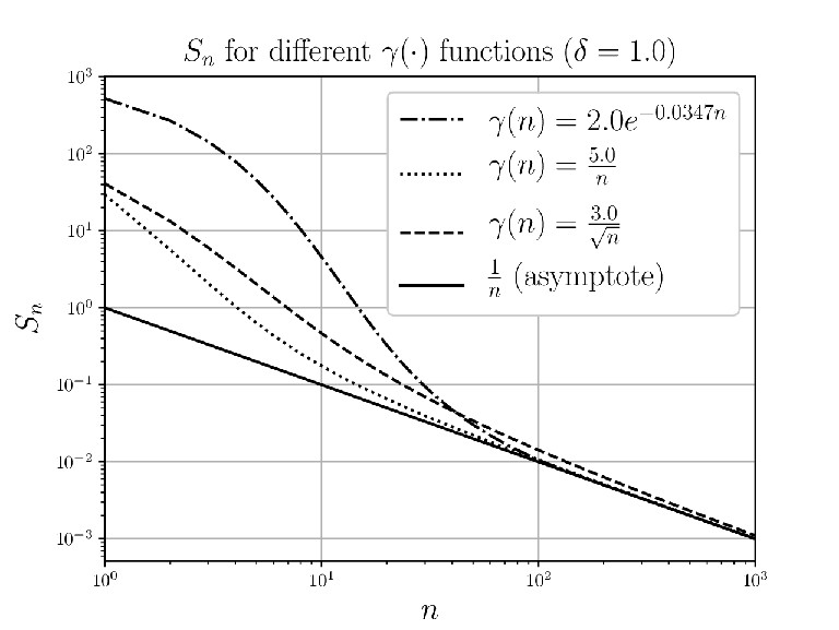
Here, we provide some numerical computations to support Theorem 4. Note that in contrast to the network-wide simulations in Fig. 3 and 4 where we have used the infectiousness functions and , we use here which captures the infectiousness for both the upper- and lower-bound Markov chains together in a single expression using (8). We consider three different functions and plot the values of computed using the recursion from (9) (with the base case from Claim 4). We plot this in Fig. 5.

Fig. 5 shows that even small changes in can cause large changes in the values of . Further, Fig. 5 may seem to indicate that even these small changes cause the mean hitting times to not converge to the same asymptote. This would be contrary to what we expect from Theorem 4. However, the reason we do not see all the three curves in Fig. 5 converge to the same asymptote is that the convergence happens extremely slowly. This is not very surprising, given that the asymptote is the function . Since the logarithmic function increases very slowly, differences between for different functions at small values of take a very long time to become insignificant, and the values become close to each other only at very large values of .
To demonstrate this, consider . We choose this function because it leads to easier analysis. Similar arguments hold for any other function as well. Substituting this into Claim 4 gives us
| (12) |
Equation (12) is quite sensitive to the value of . For example, with , we get a derivative of at . Small changes in the value of can significantly change the value of . We can use the recursion from (9) to analytically find the value of to find that is even more sensitive to the value of . Since is of the form , and asymptotically reaches , these differences in become negligible only for a very large value of .
We can verify this using Fig. 6 where we plot the values of for different functions. We see that all of them eventually reach the asymptote . This means that for large enough , the mean hitting times will all be indistinguishable from . However, we need an extremely large value of for the differences to become negligible.
VII Conclusion
We have developed a model for epidemic spread within and across population centers with state-dependent infectiousness. In this model, we directly prove (without mean-field assumptions) that there exists a sharp threshold for the curing rate such that when is more than a threshold, the epidemic dies out quickly (the mean lifetime is of logarithmic order in the initial infection size), and when is less than the threshold, the mean lifetime of the epidemic is infinite. Although is not typically something we can control, especially in the initial stages of a pandemic without vaccines or other medication, it is possible to lower the threshold by following more stringent precautions. While we do not provide prescriptive solutions for managing pandemics, we hope that this work would offer useful insights to policymakers.
While our model makes no mean-field assumptions to characterize the extinction time, we provide theoretical results only on its expected value. It is of interest to establish high-probability bounds on extinction time and characterize how strongly extinction time concentrates. Combining techniques in Claim 2 with literature on (discrete-time) Markov concentration [47, 48] might be pursued.
There is also scope for developing broader and more realistic models of state-dependent infectiousness. Empirical work suggests that people take precautions against contagions not only in response to the actual number of infections, but also to other factors like the media attention on infection prevalence [20, 21]. These models should capture infectiousness as a function of both the actual infection prevalence and the spread of awareness through (social) media.
Finally, it is important to accurately infer parameters of our model using historical and current epidemiological data so as to inform practical applications.
References
- [1] D. M. Morens and A. S. Fauci, “Emerging infectious diseases: Threats to human health and global stability,” PLoS Pathog., vol. 9, no. 7, p. e1003467, Jul. 2013.
- [2] M. D. Shirley and S. P. Rushton, “The impacts of network topology on disease spread,” Ecol. Complex., vol. 2, no. 3, pp. 287–299, Sep. 2005.
- [3] M. E. Newman, “Spread of epidemic disease on networks,” Phys. Rev. E, vol. 66, no. 1, p. 016128, Jul. 2002.
- [4] G. Giordano, F. Blanchini, R. Bruno, P. Colaneri, A. Di Filippo, A. Di Matteo, and M. Colaneri, “Modelling the COVID-19 epidemic and implementation of population-wide interventions in Italy,” Nature Med., vol. 26, no. 6, pp. 855–860, Jun. 2020.
- [5] V. Colizza, A. Barrat, M. Barthélemy, and A. Vespignani, “The modeling of global epidemics: Stochastic dynamics and predictability,” Bull. Math. Biol., vol. 68, no. 8, pp. 1893–1921, Nov. 2006.
- [6] T. Kuchler, D. Russel, and J. Stroebel, “JUE Insight: The geographic spread of COVID-19 correlates with the structure of social networks as measured by Facebook,” J. Urban Econ., p. 103314, Jan. 2021.
- [7] Y. Zhou, L. Wang, L. Zhang, L. Shi, K. Yang, J. He, B. Zhao, W. Overton, S. Purkayastha, and P. Song, “A spatiotemporal epidemiological prediction model to inform county-level COVID-19 risk in the United States,” Harvard Data Sci. Rev., Aug. 2020.
- [8] S. Gómez, A. Arenas, J. Borge-Holthoefer, S. Meloni, and Y. Moreno, “Discrete-time Markov chain approach to contact-based disease spreading in complex networks,” Europhys. Lett., vol. 89, no. 3, p. 38009, Feb. 2010.
- [9] A. Ganesh, L. Massoulié, and D. Towsley, “The effect of network topology on the spread of epidemics,” in Proc. 24th Annu. Joint Conf. IEEE Comput. Commun. Soc. (INFOCOM 2005), vol. 2, Mar. 2005, pp. 1455–1466.
- [10] F. Fagnani and L. Zino, “Diffusion of innovation in large scale graphs,” IEEE Trans. Netw. Sci. Eng., vol. 4, no. 2, pp. 100–111, 2017.
- [11] P. Van Mieghem, J. Omic, and R. Kooij, “Virus spread in networks,” IEEE/ACM Trans. Netw., vol. 17, no. 1, pp. 1–14, Jun. 2008.
- [12] F. D. Sahneh, A. Vajdi, J. Melander, and C. M. Scoglio, “Contact adaption during epidemics: A multilayer network formulation approach,” IEEE Trans. Netw. Sci. Eng., vol. 6, no. 1, pp. 16–30, Nov. 2017.
- [13] F. D. Sahneh, F. N. Chowdhury, and C. M. Scoglio, “On the existence of a threshold for preventive behavioral responses to suppress epidemic spreading,” Sci. Rep., vol. 2, no. 632, Sep. 2012.
- [14] V. Colizza and A. Vespignani, “Invasion threshold in heterogeneous metapopulation networks,” Phys. Rev. Lett., vol. 99, no. 14, p. 148701, 2007.
- [15] V. Colizza, R. Pastor-Satorras, and A. Vespignani, “Reaction–diffusion processes and metapopulation models in heterogeneous networks,” Nature Phys., vol. 3, no. 4, pp. 276–282, Apr. 2007.
- [16] V. Colizza and A. Vespignani, “Epidemic modeling in metapopulation systems with heterogeneous coupling pattern: Theory and simulations,” J. Theor. Biol., vol. 251, no. 3, pp. 450–467, 2008.
- [17] L. Wang and X. Li, “Spatial epidemiology of networked metapopulation: An overview,” Chin. Sci. Bull., vol. 59, no. 28, pp. 3511–3522, 2014.
- [18] D. Chakrabarti, Y. Wang, C. Wang, J. Leskovec, and C. Faloutsos, “Epidemic thresholds in real networks,” ACM Trans. Inf. Syst. Secur., vol. 10, no. 4, pp. 1–26, Jan. 2008.
- [19] Y. Yan, A. A. Malik, J. Bayham, E. P. Fenichel, C. Couzens, and S. B. Omer, “Measuring voluntary and policy-induced social distancing behavior during the COVID-19 pandemic,” Proc. Natl. Acad. Sci., vol. 118, no. 16, Apr. 2021.
- [20] E. P. Fenichel, N. V. Kuminoff, and G. Chowell, “Skip the trip: Air travelers’ behavioral responses to pandemic influenza,” PloS ONE, vol. 8, no. 3, p. e58249, Mar. 2013.
- [21] M. Springborn, G. Chowell, M. MacLachlan, and E. P. Fenichel, “Accounting for behavioral responses during a flu epidemic using home television viewing,” BMC Infectious Diseases, vol. 15, no. 1, pp. 1–14, Dec. 2015.
- [22] K. J. Bourassa, “State-level stay-at-home orders and objectively measured movement in the United States during the COVID-19 pandemic,” Psychosomatic Med., Dec. 2020.
- [23] S. Chang, E. Pierson, P. W. Koh, J. Gerardin, B. Redbird, D. Grusky, and J. Leskovec, “Mobility network models of COVID-19 explain inequities and inform reopening,” Nature, vol. 589, pp. 82–87, Jan. 2021.
- [24] E. P. Fenichel, C. Castillo-Chavez, M. G. Ceddia, G. Chowell, P. A. G. Parra, G. J. Hickling, G. Holloway, R. Horan, B. Morin, C. Perrings, M. Springborn, L. Velazquez, and C. Villalobos, “Adaptive human behavior in epidemiological models,” Proc. Natl. Acad. Sci., vol. 108, no. 15, pp. 6306–6311, Apr. 2011.
- [25] L. Sattenspiel, “Modeling the spread of infectious disease in human populations,” Am. J. Phys. Anthropol., vol. 33, no. S11, pp. 245–276, 1990.
- [26] Y.-C. Chen, P.-E. Lu, C.-S. Chang, and T.-H. Liu, “A time-dependent SIR model for COVID-19 with undetectable infected persons,” IEEE Trans. Netw. Sci. Eng., vol. 7, no. 4, pp. 3279–3294, Sep. 2020.
- [27] P. Holme, “Extinction times of epidemic outbreaks in networks,” PLoS ONE, vol. 8, no. 12, p. e84429, Dec. 2013.
- [28] B. S. Khatri, “Stochastic extinction of epidemics: how long would it take for SARS-CoV-2 to die out without herd immunity?” medRxiv, Aug. 2020.
- [29] P. Holme and L. Tupikina, “Epidemic extinction in networks: insights from the smallest graphs,” New J. Phys., vol. 20, no. 11, p. 113042, Nov. 2018.
- [30] J. Hindes and I. B. Schwartz, “Epidemic extinction and control in heterogeneous networks,” Phys. Rev. Lett., vol. 117, no. 2, p. 028302, Jul. 2016.
- [31] H. Chen, F. Huang, H. Zhang, and G. Li, “Epidemic extinction in a generalized susceptible-infected-susceptible model,” J. Stat. Mech., vol. 2017, no. 1, p. 013204, Jan. 2017.
- [32] F. Ball and T. House, “Heterogeneous network epidemics: real-time growth, variance and extinction of infection,” J. Math. Biol., vol. 75, no. 3, pp. 577–619, Sep. 2017.
- [33] C. Kim, S. H. Cheon, K. Choi, C.-H. Joh, and H.-J. Lee, “Exposure to fear: Changes in travel behavior during MERS outbreak in Seoul,” KSCE J. Civ. Eng., vol. 21, no. 7, pp. 2888–2895, Nov. 2017.
- [34] A. E. Brouwer and W. H. Haemers, Spectra of Graphs. Springer Science & Business Media, 2011.
- [35] G. B. Thomas, Jr. and R. L. Finney, Calculus and Analytic Geometry, 9th ed. Addison-Wesley Publishing Company, 1996.
- [36] V. A. Malyšev and M. V. Men’šikov, “Ergodicity, continuity and analyticity of countable markov chains,” Trudy Moskovskogo Matematicheskogo Obshchestva, vol. 39, pp. 3–48, 1979, English Transl. in Trans. Moscow Math. Soc., 1981.
- [37] S. I. Resnick, Adventures in Stochastic Processes. Springer Science & Business Media, 1992.
- [38] F. G. Foster, “On the stochastic matrices associated with certain queuing processes,” Ann. Math. Stat., vol. 24, no. 3, pp. 355–360, Sep. 1953.
- [39] R. Srikant and L. Ying, Communication Networks: an Optimization, Control, and Stochastic Networks Perspective. Cambridge, United Kingdom: Cambridge University Press, 2013.
- [40] D. W. S. Wong and Y. Li, “Spreading of COVID-19: Density matters,” PLoS ONE, vol. 15, no. 12, p. e0242398, Dec. 2020.
- [41] L. R. Varshney and R. Socher, “COVID-19 growth rate decreases with social capital,” medRxiv, Apr. 2020.
- [42] A. J. Schwenk, “Tight bounds on the spectral radius of asymmetric nonnegative matrices,” Linear Algebra Appl., vol. 75, pp. 257–265, Mar. 1986.
- [43] R. Bhatia, Matrix Analysis. New York: Springer, 1997.
- [44] S. M. Ross, Introduction to Probability Models. London, United Kingdom: Academic Press, 2019.
- [45] D. T. Gillespie, “Exact stochastic simulation of coupled chemical reactions,” J. Phys. Chem., vol. 81, no. 25, pp. 2340–2361, Dec. 1977.
- [46] F. Johansson et al., mpmath: a Python library for arbitrary-precision floating-point arithmetic (version 1.0.0), Sep. 2017. [Online]. Available: http://mpmath.org/
- [47] T. Kötzing, “Concentration of first hitting times under additive drift,” Algorithmica, vol. 75, no. 3, pp. 490–506, Jul. 2016.
- [48] D. Paulin, “Concentration inequalities for Markov chains by Marton couplings and spectral methods,” Elec. J. Prob., vol. 20, pp. 1–32, Jan. 2015.
| Akhil Bhimaraju received the B.Tech. and M.Tech. degrees in electrical engineering from the Indian Institute of Technology Madras in 2020. He is currently a Ph.D. student with the department of electrical and computer engineering and the Coordinated Science Laboratory at the University of Illinois Urbana–Champaign. His research interests include mathematical modeling of engineering problems. |
| Avhishek Chatterjee received the Ph.D. degree in electrical and computer engineering from The University of Texas at Austin in 2015. From 2015 to 2017, he was a Post–Doctoral Research Associate with the Coordinated Science Laboratory, University of Illinois Urbana–Champaign. He is currently an Assistant Professor with the Department of Electrical Engineering, IIT Madras. His research interests lie in theoretical studies of dynamics, optimal designs, and operations of stochastic networks. |
| Lav R. Varshney (S’00–M’10–SM’15) received the B.S. degree (magna cum laude) with honors in electrical and computer engineering from Cornell University, Ithaca, NY, USA, in 2004, and the S.M., E.E., and Ph.D. degrees in electrical engineering and computer science from the Massachusetts Institute of Technology, Cambridge, MA, USA, in 2006, 2008, and 2010, respectively. He is currently an associate professor of electrical and computer engineering, with further affiliations in computer science, industrial engineering, neuroscience, digital agriculture, and personalized nutrition with the University of Illinois Urbana–Champaign. He is also a computational scientist with Brookhaven National Laboratory, Upton, NY, USA. |
Appendix A Proof of Claim 1
The following proof that we provide here closely resembles the proof of [9, Theorem 3.1]. However, since we are not interested in the exact constant like [9], we avoid the use of matrix exponentials seen there. The rates of (1) (with constant and ) give us the following differential equation:
where is the identity matrix (of correct size). Multiply each side of the equation with ( is the eigenvector of corresponding to ). This gives us
| (13) |
Since is an eigenvector of with eigenvalue , and an eigenvector of with eigenvalue (every vector is an eigenvector of with eigenvalue ), (13) gives us
This is a differential equation in terms of , and solving it gives us
Let and denote the maximum and minimum elements of , i.e., and . Since , is strictly positive. This gives us
| (14) |
The mean hitting time can be written as
for any . The last inequality follows from the fact that since it is a probability (which gives the first term), and the Markov inequality which gives us (for the second term).
Appendix B Proof of Claim 2
Divide the time axis into intervals of unit length. Given any (finite) , if the number of transitions in all intervals preceding and including is finite, then the cardinality of the set is finite. Further, this cardinality is unique for each , allowing us to map to this unique natural number plus one. Thus we get an injective mapping (if the number of transitions in each interval is finite).
At the start of the interval, assume that the Markov chain starts in state with . The probability that there are at least transitions in the interval satisfies
| (15) |
where are the amounts of time it takes to transition out of the first states starting from at the beginning of the interval.
Since the total rate of transition rate out of is given by , the total transition rate out of any state with at most infections is less than or equal to . Recall that , , and is the maximum degree among nodes of . Define .
So in the worst case, which gives the greatest probability on the right side of (15), we have . This gives us
If as , then the probability that there are infinite transitions in the interval goes to . But this is equivalent to as .
This gives us
For a large enough , we can make arbitrarily close to . This implies
where is chosen to be large enough so that is at most away from for all . The sum goes to infinity because the sum of the harmonic series goes to infinity. Since this ensures that the Markov chain only has a finite number of transitions in any interval, it concludes the proof.
Appendix C Proof of Corollary 1
We need to show that
Recall that the spectral radius of a matrix is defined as the maximum absolute value of the eigenvalues of the matrix. Let be an eigenvalue of . This yields
or
This implies is an eigenvalue of for every eigenvalue of . The Perron-Frobenius theorem (see [34]) guarantees that there exists a positive eigenvalue of which has the maximum absolute value. Thus the maximum absolute value of is .
Appendix D Spectral Radius of Sum of Symmetric and Diagonal Matrices
In this appendix, we prove a special case of Weyl’s inequality which suffices for the purposes of this paper. We state this formally in Claim 7.
Claim 7.
Let be any nonnegative symmetric matrix and be any nonnegative diagonal matrix. Then
where denotes the spectral radius.
Proof:
Recall that the spectral radius of a matrix is the maximum absolute value of the eigenvalues of the matrix. For symmetric matrices, the eigenvalues are all real, and since and are nonnegative, the Perron-Frobenius theorem ensures that there is a positive eigenvalue which has the maximum absolute value. Thus we have
Let be the unit vector which maximizes , i.e., . This gives
where the second inequality follows since is the least value of subject to since is a diagonal matrix. This proves the lower bound of Claim 7.
For the upper bound, we have
which concludes the proof. ∎
Appendix E Proof of Claim 6
Since , for any , we can find an such that for all , . Let denote the time it takes to go from infections to infections (for the first time). Then we have
But the birth rate of the Markov chain between and is less than (from the definition of ). So should be less than the expected time to go from to in a Markov chain where all the birth rates are . This gives us (using Claim 5):
Since depends only on given a , this concludes the proof for the second inequality.
The first inequality is relatively straightforward since is the lower bound in Claim 5 if the birth rate was throughout.
Appendix F Extinction time exponential in equilibrium point
For simplicity, we just consider the upper- and lower-bound Markov chains using the rates from (8) defined using the function here. We expect similar arguments to hold for the network-wide epidemic as well. Let for all and for all . Since this satisfies the condition of Theorem 4, we are guaranteed that the mean epidemic extinction time is logarithmic in the initial infection size. However, the mean extinction time also turns out to be exponential in , the “equilibrium point,” or the size of the epidemic where the rate of infectiousness goes below the curing rate .
To see this, substitute these values into the expression for from Claim 4. We get
If or are large enough, is greater than an exponential of the form for some . This implies that the mean die-out time is exponential in the equilibrium point .