Robust Models Are More Interpretable
Because Attributions Look Normal

Zifan Wang Matt Fredrikson & Anupam Datta Affiliation: Carnegie Mellon Univeristy Affiliation: Pittsburgh, PA 15213, USA Email: zifan@cmu.edu

Abstract

Recent work has found that adversarially-robust deep networks used for image classification are more interpretable: their feature attributions tend to be sharper, and are more concentrated on the objects associated with the image’s ground-truth class. We show that smooth decision boundaries play an important role in this enhanced interpretability, as the model’s input gradients around data points will more closely align with boundaries’ normal vectors when they are smooth. Thus, because robust models have smoother boundaries, the results of gradient-based attribution methods, like Integrated Gradients and DeepLift, will capture more accurate information about nearby decision boundaries. This understanding of robust interpretability leads to our second contribution: boundary attributions, which aggregate information about the normal vectors of local decision boundaries to explain a classification outcome. We show that by leveraging the key factors underpinning robust interpretability, boundary attributions produce sharper, more concentrated visual explanations—even on non-robust models. Any example implementation can be found at https://github.com/zifanw/boundary.

1 Introduction

Feature attribution methods are widely used to explain the predictions of neural networks (Binder et al. 2016; Dhamdhere et al. 2019; Fong & Vedaldi 2017; Leino et al. 2018; Montavon et al. 2015; Selvaraju et al. 2017; Shrikumar et al. 2017; Simonyan et al. 2013; Smilkov et al. 2017; Springenberg et al. 2014; Sundararajan et al. 2017). By assigning an importance score to each input feature of the model, these techniques help to focus attention on parts of the data most responsible for the model’s observed behavior. Recent work (Croce et al. 2019; Etmann et al. 2019) has observed that feature attributions in adversarially-robust image models, when visualized, tend to be more interpretable—the attributions correspond more clearly to the discriminative portions of the input.

One way to explain the observation relies on the fact that robust models do not make use of non-robust features (Ilyas et al. 2019) whose statistical meaning can change with small, imperceptible changes in the source data. Thus, by using only robust features to predict, these models naturally tend to line up with visibly-relevant portions of the image. Etmann et al. 2019 take a different approach, showing that the gradients of robust models’ outputs more closely align with their inputs, which explains why attributions on image models are more visually interpretable.

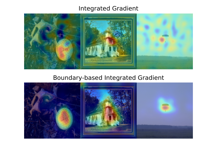
In this paper, we build on this geometric understanding of robust interpretability. With both analytical (Sec. 3) and empirical (Sec. 5) results, we show that the gradient of the model with respect to its input, which is the basic building block of all gradient-based attribution methods, tends to be more closely aligned with the normal vector of a nearby decision boundary in robust models than in “normal” models. Leveraging this understanding, we propose Boundary-based Saliency Map (BSM) and Boundary-based Integrated Gradient (BIG), two variants of boundary attributions (Sec. 4), which base attributions on information about nearby decision boundaries (see an illustration in Fig. 1(a)). While BSM provides theoretical guarantees in the closed-form, BIG generates both quantitatively and qualitatively better explanations. We show that these methods satisfy several desireable formal properties, and that even on non-robust models, the resulting attributions are more focused (Fig. 1(b)) and less sensitive to the “baseline” parameters required by some attribution methods.

To summarize, our main contributions are as follows. (1) We present an analysis that sheds light on the previously-observed phenomeon of robust interpretability, showing that alignment between the normal vectors of decision boundaries and models’ gradients is a key ingredient (Proposition 1, Theorem 1). (2) Motivated by our analysis, we introduce boundary attributions, which leverage the connection between boundary normal vectors and gradients to yield explanations for non-robust models that carry over many of the favorable properties that have been observed of explanations on robust models. (3) We empirically demonstrate that one such type of boundary attribution, called Boundary-based Integrated Gradients (BIG), produces explanations that are more accurate than prior attribution methods (relative to ground-truth bounding box information), while mitigating the problem of baseline sensitivity that is known to impact applications of Integrated Gradients Sundararajan et al. 2017 (Section 6).

2 Background

We begin by introducing our notations. Throughout the paper we use italicized symbols $x$ to denote scalar quantities and bold-face $\mathbf{x}$ to denote vectors. We consider neural networks with ReLU as activations prior to the top layer, and a softmax activation at the top. The predicted label for a given input $\mathbf{x}$ is given by $F(\mathbf{x})=\arg\max_{c}f_{c}(\mathbf{x}),\mathbf{x}\in\mathbb{R}^{d}$ , where $F(\mathbf{x})$ is the predicted label and $f_{i}(\mathbf{x})$ is the output on the class $i$ . As the softmax layer does not change the ranking of neurons in the top layer, we will assume that $f_{i}(\mathbf{x})$ denotes the pre-softmax score. Unless otherwise noted, we use $||\mathbf{x}||$ to denote the $\ell_{2}$ norm of $\mathbf{x}$ , and the $\ell_{2}$ neighborhood centered at $\mathbf{x}$ with radius $\epsilon$ as $B(\mathbf{x},\epsilon)$ .

Explainability.

Feature attribution methods are widely-used to explain the predictions made by DNNs, by assigning importance scores for the network’s output to each input feature. Conventionally, scores with greater magnitude indicate that the corresponding feature was more relevant to the predicted outcome. We denote feature attributions by $\mathbf{z}=g(\mathbf{x},f),\mathbf{z},\mathbf{x}\in\mathbb{R}^{d}$ . When $f$ is clear from the context, we simply write $g(\mathbf{x})$ . While there is an extensive and growing literature on attribution methods, our analysis will focus closely on the popular gradient-based methods, Saliency Map (Simonyan et al. 2013), Integrated Gradient (Sundararajan et al. 2017) and Smooth Gradient (Smilkov et al. 2017), shown in Defs 1-3.

Definition 1 (Saliency Map (SM))

The Saliency Map $g_{\text{S}}(\mathbf{x})$ is given by $g_{\text{S}}(\mathbf{x}):=\frac{\partial f(\mathbf{x})}{\partial\mathbf{x}}$ .

Definition 2 (Integrated Gradient (IG))

Given a baseline input $\mathbf{x}_{b}$ , the Integrated Gradient $g_{\text{IG}}(\mathbf{x};\mathbf{x}_{b})$ is given by $g_{\text{IG}}(\mathbf{x};\mathbf{x}_{b}):=(\mathbf{x}-\mathbf{x}_{b})\int^{1}_{0}\frac{\partial f((\mathbf{x}-\mathbf{x}_{b})t+\mathbf{x}_{b})}{\partial\mathbf{x}}dt$ .

Definition 3 (Smooth Gradient (SG))

Given a zero-centered Gaussian distribution $\mathcal{N}$ with a standard deviation $\sigma$ , the Smooth Gradient $g_{\text{SG}}(\mathbf{x};\sigma)$ is given by $g_{\text{SG}}(\mathbf{x};\sigma):=\mathbb{E}_{\bm{\epsilon}\sim\mathcal{N}(\mathbf{0},\sigma^{2}I)}\frac{\partial f(\bm{\alpha}+\bm{\epsilon})}{\partial\mathbf{x}}$ .

Besides, we will also include results from DeepLIFT (Shrikumar et al. 2017) and grad $\times$ input (element-wise multiplication between Saliency Map and the input) (Simonyan et al. 2013) in our empirical evaluation. As we show in Section 3.2, Defs 1-3 satisfy axioms that relate to the local linearity of ReLU networks, and in the case of randomized smoothing (Cohen et al. 2019), their robustness to input perturbations. We further discuss these methods relative to others in Sec. 7.

Robustness. Two relevant concepts about adversarial robustness will be used in this paper: prediction robustness that the model’s output label remains unchanged within a particular $\ell_{p}$ norm ball and attribution robustness that the feature attributions are similar within the same ball. Recent work has identified the model’s Lipschitz continuity as a bridge between these two concepts (Wang et al. 2020c) and some loss functions in achieving prediction robustness also bring attribution robustness (Chalasani et al. 2020). We refer to robustness as prediction robustness if not otherwise noted.

3 Explainability, Decision Boundaries, and Robustness

In this section, we begin by discussing the role of decision boundaries in constructing explanations of model behavior via feature attributions. We first illustrate the key relationships in the simpler case of linear models, which contain exactly one boundary, and then generalize to piecewise-linear classifiers as they are embodied by deep ReLU networks. We then show how local robustness causes attribution methods to align more closely with nearby decision boundaries, leading to explanations that better reflect these relationships.

3.1 Attributions for linear models

Consider a binary classifier $C(\mathbf{x})=\text{sign}(\mathbf{w}^{\top}\mathbf{x}+\mathbf{b})$ that predicts a label $\{-1,1\}$ (ignoring “tie” cases where $C(\mathbf{x})=0$ , which can be broken arbitrarily). In its feature space, $C(\mathbf{x})$ is a hyperplane $H$ that separates the input space into two open half-spaces $S_{1}$ and $S_{2}$ (see Fig. 2(a)). Accordingly, the normal vector $\hat{\mathbf{n}}$ of the decision boundary is the only vector that faithfully explains the model’s classification while other vectors, while they may describe directions that lead to positive changes in the model’s output score, are not faithful in this sense (see $\mathbf{v}$ in Fig. 2(a) for an example). In practice, to assign attributions for predictions made by $C$ , SM, SG, and the integral part of IG (see Sec. 2) return a vector characterized by $\mathbf{z}=k_{1}\hat{\mathbf{n}}+k_{2}$ (Ancona et al. 2018), where $k_{1}\ \neq 0$ and $k_{2}\in\mathbb{R}$ , regardless of the input $\mathbf{x}$ that is being explained. In other words, these methods all measure the importance of features by characterizing the model’s decision boundary, and are equivalent up to the scale and position of $\hat{\mathbf{n}}$ .

3.2 Generalizing to piecewise-linear boundaries

In the case of a piecewise-linear model, such as a ReLU network, the decision boundaries comprise a collection of hyperplane segments that partition the feature space, as in $H_{1},H_{2}$ and $H_{3}$ in the example shown in Figure 2(b). Because the boundary no longer has a single well-defined normal, one intuitive way to extend the relationship between boundaries and attributions developed in the previous section is to capture the normal vector of the closest decision boundary to the input being explained. However, as we show in this section, the methods that succeeded in the case of linear models (SM, SG, and the integral part of IG) may in fact fail to return such attributions in the more general case of piecewise-linear models, but local robustness often remedies this problem. We begin by reviewing key elements of the geometry of ReLU networks (Jordan et al. 2019).

ReLU activation polytopes. For a neuron $u$ in a ReLU network $f(\mathbf{x})$ , we say that its status is ON if its pre-activation $u(\mathbf{x})\geq 0$ , otherwise it is OFF. We can associate an activation pattern denoting the status of each neuron for any point $\mathbf{x}$ in the feature space, and a half-space $A_{u}$ to the activation constraint $u(\mathbf{x})\geq 0$ . Thus, for any point $\mathbf{x}$ the intersection of the half-spaces corresponding to its activation pattern defines a polytope $P$ (see Fig. 2(b)), and within $P$ the network is a linear function such that $\forall\mathbf{x}\in P,f(\mathbf{x})=\mathbf{w}_{P}^{\top}\mathbf{x}+b_{P}$ , where the parameters $\mathbf{w}_{p}$ and $b_{P}$ can be computed by differentiation (Fromherz et al. 2021). Each facet of $P$ (dashed lines in Fig. 2(b)) corresponds to a boundary that “flips” the status of its corresponding neuron. Similar to activation constraints, decision boundaries are piecewise-linear because each decision boundary corresponds to a constraint $f_{i}(\mathbf{x})\geq f_{j}(\mathbf{x})$ for two classes $i,j$ (Fromherz et al. 2021; Jordan et al. 2019).

Gradients might fail. Saliency maps, which we take to be simply the gradient of the model with respect to its input, can thus be seen as a way to project an input onto a decision boundary. That is, a saliency map is a vector that is normal to a nearby decision boundary segment. However, as others have noted, a saliency map is not always normal to any real boundary segment in the model’s geometry (see the left plot of Fig. 2(c)), because when the closest boundary segment is not within the activation polytope containing $\mathbf{x}$ , the saliency map will instead be normal to the linear extension of some other hyperplane segment (Fromherz et al. 2021). In fact, the fact that iterative gradient descent typically outperforms the Fast Gradient Sign Method (Goodfellow et al. 2015) as an attack demonstrates that this is often the case.

When gradients succeed. While saliency maps may not be the best approach in general for capturing information about nearby segments of the model’s decision boundary, there are cases in which it serves as a good approximation. Recent work has proposed using the Lipschitz continuity of an attribution method to characterize the difference between the attributions of an input $\mathbf{x}$ and its neighbors within a $\ell_{p}$ ball neighborhood (Def. 4) (Wang et al. 2020c). This naturally leads to Proposition 1, which states that the difference between the saliency map at an input and the correct normal to the closest boundary segment is bounded by the distance to that segment.

Definition 4 (Attribution Robustness)

An attribution method $g(\mathbf{x})$ is $(\lambda,\delta)$ -locally robust at the evaluated point $\mathbf{x}$ if $\forall\mathbf{x}^{\prime}\in B(\mathbf{x},\delta),||g(\mathbf{x}^{\prime})-g(\mathbf{x})||\leq\lambda||\mathbf{x}^{\prime}-\mathbf{x}||$ .

Proposition 1

Suppose that $f$ has a $(\lambda,\delta)$ -robust saliency map $g_{\text{S}}$ at $\mathbf{x}$ , $\mathbf{x}^{\prime}$ is the closest point on the closest decision boundary segment to $\mathbf{x}$ and $||\mathbf{x}^{\prime}-\mathbf{x}||\leq\delta$ , and that $\mathbf{n}$ is the normal vector of that boundary segment. Then $||\mathbf{n}-g_{\text{S}}(\mathbf{x})||\leq\lambda||\mathbf{x}-\mathbf{x}^{\prime}||$ .

Proposition 1 therefore provides the following insight: for networks that admit robust attributions (Chen et al. 2019; Wang et al. 2020c), the saliency map is a good approximation to the boundary vector. As prior work has demonstrated the close correspondence between robust prediction and robust attributions (Wang et al. 2020c; Chalasani et al. 2020), this in turn suggests that explanations on robust models will more closely resemble boundary normals.

As training robust models can be expensive, and may not come with guarantees of robustness, post-processing techniques like randomized smoothing (Cohen et al. 2019), have been proposed as an alternative. Dombrowski et al. 2019 noted that models with softplus activations ( $\mathbf{y}=1/\beta\log(1+\exp{(\beta\mathbf{x})})$ ) approximate smoothing, and in fact give an exact correspondence for single-layer networks. Combining these insights, we arrive at Theorem 1, which suggests that the saliency map on a smoothed model approximates the closest boundary normal vector well; the similarity is inversely proportional to the standard deviation of the noise used to smooth the model.

Theorem 1

Let $m(\mathbf{x})$ be a one-layer ReLU network, and denote its smoothed counterpart under the Gaussian with standard deviation $\sigma$ as $m_{\sigma}(\mathbf{x})$ . and $g(\mathbf{x})$ be the saliency map for $m_{\sigma}(\mathbf{x})$ . If $\mathbf{x}^{\prime}$ is the closest adversarial example to $\mathbf{x}$ , and $\forall\mathbf{x}^{\prime\prime}\in B(\mathbf{x},||\mathbf{x}-\mathbf{x}^{\prime}||).||g(\mathbf{x}^{\prime\prime})||\geq c$ , then the following statement holds: $||g(\mathbf{x})-g(\mathbf{x}^{\prime})||\lessapprox\lambda$ where $\lambda\propto O(\frac{1}{\sigma})$ .

Theorem 1 suggests that when randomized smoothing is used, the normal vector of the closest decision boundary segment and the saliency map are similar, and this similarity increases with the smoothness of the model’s boundaries. Because the saliency map for a smoothed model is equivalent to smooth gradient of its non-smooth counterpart (Wang et al. 2020c), the smooth gradient is a better choice whenever computing the exact boundary is too expensive in a standard model. We provide empirical validation of this in Figure 10.

4 Boundary-Based Attribution

Without the properties introduced by robust learning or randomized smoothing, the local gradient, i.e. saliency map, may not be a good approximation of decision boundaries. In this section, we build on the insights of our analysis to present a set of novel attribution methods that explicitly incorporate the normal vectors of nearby boundary segments. Importantly, these attribution methods can be applied to models that are not necessarily robust, to derive explanations that capture many of the beneficial properties of explanations for robust models.

Using the normal vector of the closest decision boundary to explain a classifier naturally leads to Definition 5, which defines attributions directly from the normal of the closest decision boundary.

Definition 5 (Boundary-based Saliency Map (BSM))

Given $f$ and an input $\mathbf{x}$ , we define Boundary-based Saliency Map $B_{\text{S}}(\mathbf{x})$ as follows: $B_{\text{S}}(\mathbf{x})\stackrel{{\scriptstyle\smash{\scriptscriptstyle\mathrm{def}}}}{{=}}\partial f_{c}(\mathbf{x}^{\prime})/\partial\mathbf{x}^{\prime}$ , where $\mathbf{x}^{\prime}$ is the closest adversarial example to $\mathbf{x}$ , i.e. $c=F(\mathbf{x})\neq F(\mathbf{x}^{\prime})$ and $\forall\mathbf{x}_{m}.||\mathbf{x}_{m}-\mathbf{x}||<||\mathbf{x}^{\prime}-\mathbf{x}||\rightarrow F(\mathbf{x})=F(\mathbf{x}_{m})$ .

Incorporating More Boundaries.

The main limitation of using Definition 5 as a local explanation is obvious: the closest decision boundary only captures one segment of the entire decision surface. Even in a small network, there will be numerous boundary segments in the vicinity of a relevant point. Taking inspiration from Integrated Gradients, Definition 6 proposes the Boundary-based Integrated Gradient (BIG) by aggregating the attributions along a line between the input and its closest boundary segment.

Definition 6 (Boundary-based Integrated Gradient(BIG))

Given $f$ , Integrated Gradient $g_{\text{IG}}$ and an input $\mathbf{x}$ , we define Boundary-based Integrated Gradient $B_{\text{S}}(\mathbf{x})$ as follows: $B_{\text{IG}}(\mathbf{x}):=g_{\text{IG}}(\mathbf{x};\mathbf{x}^{\prime})$ , where $\mathbf{x}$ is the nearest adversarial example to $\mathbf{x}$ , i.e. $c=F(\mathbf{x})\neq F(\mathbf{x}^{\prime})$ and $\forall\mathbf{x}_{m}.||\mathbf{x}_{m}-\mathbf{x}||<||\mathbf{x}^{\prime}-\mathbf{x}||\rightarrow F(\mathbf{x})=F(\mathbf{x}_{m})$ .

Geometric View of BIG.

BIG explores a linear path from the boundary point to the target point. Because points on this path are likely to traverse different activation polytopes, the gradient of intermediate points used to compute $g_{\text{IG}}$ are normals of linear extensions of their local boundaries. As the input gradient is identical within a polytope $P_{i}$ , the aggregate computed by BIG sums each gradient $\mathbf{w}_{i}$ along the path and weights it by the length of the path segment intersecting with $P_{i}$ . In other words, one may view IG as an exploration of the model’s global geometry that aggregates all boundaries from a fixed reference point, whereas BIG explores the local geometry around $\mathbf{x}$ . In the former case, the global exploration may reflect boundaries that are not particularly relevant to model’s observed behavior at a point, whereas the locality of BIG may aggregate boundaries that are more closely related (a visualization is shown in Fig. 1(a)).

Finding nearby boundaries. Finding the exact closest boundary segment is identical to the problem of certifying local robustness (Fromherz et al. 2021; Jordan et al. 2019; Kolter & Wong 2018; Lee et al. 2020; Leino et al. 2021b; Tjeng et al. 2019; Weng et al. 2018), which is NP-hard for piecewise-linear models (Sinha et al. 2020). To efficiently find an approximation of the closest boundary segment, we leverage and ensemble techniques for generating adversarial examples, i.e. PGD (Madry et al. 2018), AutoPGD (Croce & Hein 2020) and CW (Carlini & Wagner 2017), and use the closest one found given a time budget. The details of our implementation are discussed in Section 5, where we show that this yields good results in practice.

5 Evaluation

CIFAR10	standard		$\ell_{2}\|0.5$
SM-BSM.	59.96		1.23
IG-AGI	28.20		1.43
IG-BIG	31.22		2.73
ImageNet	standard	$\ell_{2}\|3.0$	$\ell_{\infty}\|\frac{4}{255}$	$\ell_{\infty}\|\frac{8}{255}$
SM-BSM	8.48	0.41	2.25	1.61
IG-AGI	13.52	0.36	1.19	0.86
IG-BIG	17.07	0.69	1.74	1.45

(a)

Corr.	Loc.	EG	PP	Con.
SM-BSM	0.40	0.46	-0.19	0.07
IG-AGI	0.24	0.25	0.05	-0.03
IG-BIG	0.35	0.30	0.20	-0.03

(b)

Figure 3: (a):

\ell_{2}

differences between SM, IG and their boundary variants for robust models. The heading of each column reports the respective training epsilon and the corresponding

\ell_{p}

norm constraint; Appendix B.4 reports the corresponding boxplot. (b): Linear correlation coefficients between the alignment of SM and IG with nearby boundary vectors, and the localization metrics. For each row starting with

\mathbf{X}

Y

, the alignment is defined as

-||\mathbf{X}-Y||

. For each column, the localization results are measured with approach in bold font, a.k.a

\mathbf{X}

Model	Metrics	BIG	BSM	AGI	SM	GTI	SG	IG	DeepLIFT
	Loc.	0.38	0.33	0.33	0.33	0.35	0.34	0.34	0.34
standard	EG	0.54	0.47	0.48	0.47	0.46	0.55	0.5	0.49
	PP	0.87	0.50	0.58	0.50	0.50	0.50	0.51	0.53
	Con.	4.35	3.88	4.01	3.92	3.94	4.06	3.97	3.93
	Loc.	0.39	0.33	0.39	0.33	0.33	0.34	0.33	0.33
$\ell_{2}\|3.0$	EG	0.74	0.6	0.64	0.6	0.63	0.62	0.65	0.64
	PP	0.92	0.50	0.88	0.50	0.55	0.51	0.65	0.77
	Con.	5.03	4.12	4.32	4.10	4.25	4.23	4.37	4.34

Table 1: Results of several attribution methods over 1500 images of IamgeNet using a standard and robust ResNet50 (training

\epsilon

is reported in the first column). BIG: Boundary-based Integrated Gradient. BSM: Boundary-based Saliency Map. AGI: Adversarial Gradient Integration. SM: Saliency Map. GTI: grad

\times

input. SG: Smoothed Gradient. IG: Integrated Gradient. See Appendix E for the corresponding boxplot.

In this section, we first validate that the attribution vectors are more aligned to normal vectors of nearby boundaries in robust models(Fig. 3(a)). We secondly show that boundary-based attributions provide more “accurate” explanations – attributions highlight features that are actually relevant to the label – both visually (Fig. 4 and 5) and quantitatively (Table 1). Finally, we show that in a standard model, whenever attributions more align with the boundary attributions, they are more “accurate”.

General Setup. We conduct experiments over two data distributions, ImageNet (Russakovsky et al. 2015) and CIFAR-10 (Krizhevsky et al.). For ImageNet, we choose 1500 correctly-classified images from ImageNette (Howard), a subset of ImageNet, with bounding box area less than 80% of the original source image. For CIFAR-10, We use 5000 correctly-classified images. All standard and robust deep classifiers are ResNet50. All weights are pretrained and publicly available (Engstrom et al. 2019). Implementation details of the boundary search (by ensembling the results of PGD, CW and AutoPGD) and the hyperparameters used in our experiments, are included in Appendix B.2.

5.1 Robustness $\rightarrow$ Boundary Alignment

In this subsection, we show that SM and IG better align with the normal vectors of the decision boundaries in robust models. For SM, we use BSM as the normal vectors of the nearest decision boundaries and measure the alignment by the $\ell_{2}$ distance between SM and BSM following Proposition 1. For IG, we use BIG as the aggregated normal vectors of all nearby boundaries because IG also incorporates more boundary vectors. Recently, Pan et al. 2021 also provides Adversarial Gradient Integral (AGI) as an alternative way of incorporating the boundary normal vectors into IG. We first use both BIG and AGI to measure how well IG aligns with boundary normals and later compare them in Sec. 5.2, followed by a formal discussion in Sec. 7.

Aggregated results for standard models and robust models are shown in Fig. 3(a). It shows that adversarial training with bigger $\epsilon$ encourages a smaller difference between the difference between attributions and their boundary variants. Particularly, using $\ell_{2}$ norm and setting $\epsilon=3.0$ are most effective for ImageNet compared to $\ell_{\infty}$ norm bound. One possible explanation is that the $\ell_{2}$ space is special because training with $\ell_{\infty}$ bound may encourage the gradient to be more Lipschitz in $\ell_{1}$ because of the duality between the Lipschitzness and the gradient norm, whereas $\ell_{2}$ is its own dual.

5.2 Boundary Attribution $\rightarrow$ Better Localization

In this subsection, we show boundary attributions (BSM, BIG and AGI) better localize relevant features. Besides SM, IG and SG, we also focus on other baseline methods including Grad $\times$ Input (GTI) (Simonyan et al. 2013) and DeepLIFT (rescale rule only) (Shrikumar et al. 2017) that are reported to be more faithful than other related methods (Adebayo et al. 2018; Adebayo et al. 2020).

In an image classification task where ground-truth bounding boxes are given, we consider features within a bounding box as more relevant to the label assigned to the image. Our evaluation is performed over ImageNet only because no bounding box is provided for CIFAR-10 data. The metrics used for our evaluation are: 1) Localization (Loc.) (Chattopadhyay et al. 2017) evaluates the intersection of areas with the bounding box and pixels with positive attributions; 2) Energy Game (EG) (Wang et al. 2020a) instead evaluates computes the portion of attribute scores within the bounding box. While these two metrics are common in the literature, we propose the following additional metrics: 3)Positive Percentage (PP) evaluates the portion of positive attributions in the bounding box because a naive assumption is all features within bounding boxes are relevant to the label (we will revisit this assumption in Sec. 6); and 4) Concentration (Con.) sums the absolute value of attribution scores over the distance between the “mass” center of attributions and each pixel within the bounding box. Higher Loc., EG, PP and Con. are better results. We provide formal details for the above metrics in Appendix B.1.

We show the average scores for ResNet50 models in Table 1 where the corresponding boxplots can be found in Appendix B.4. BIG is noticeably better than other methods on Loc. EG, PP and Con. scores for both robust and standard models and matches the performance of SG on EG for a standard model. Notice that BSM is not significantly better than others in a standard model, which confirms our motivation of BIG – that we need to incorporate more nearby boundaries because a single boundary may not be sufficient to capture the relevant features.

We also measure the correlation between the alignment of SM and BSM with boundary normals and the localization abilities, respectively. For SM, we use BSM to represent the normal vectors of the boundary. For IG, we use AGI and BIG. For each pair $\mathbf{X}$ - $Y$ in $\{\text{{SM}-BSM, {IG}-AGI, {IG}-BIG}\}$ , we measure the empirical correlation coefficient between $-||\mathbf{X}-Y||_{2}$ and the localization scores of $\mathbf{X}$ in a standard ResNet50 and the result is shown in Fig. 3(b). Our results suggest that when the attribution methods better align with their boundary variants, they can better localize the relevant features in terms of the Loc. and EG. However, PP and Con. have weak and even negative correlations. One possible explanation is that the high PP and Con. of BIG and AGI compared to IG (as shown in Table 1) may also come from the choice of the reference points. Namely, compared to a zero vector, a reference point on the decision boundary may better filter out noisy features.

We end our evaluations by visually comparing the proposed method, BIG, against all other attribution methods for the standard ResNet50 in Fig. 4 and for the robust ResNet50 in Fig. 5, which demonstrates that BIG can easily and efficiently localize features that are relevant to the prediction. More visualizaitons can be found in the Appendix E.

Summary. Taken together, we close the loop and empirical show that standard attributions in robust models are visually more interpretable because they better capture the nearby decision boundaries. Thefore, the final take-away from our analitical and empirical results is if more resources are devoted to training robust models, effectively identical explanations can be obtained using much less costly standard gradient-based methods, i.e. IG.

6 Discussion

Properties	black IG	AGI	BIG
Boundary-based	✗	✓	✓
Boundary Search	N/A	PGD	Any
Geometry	Global	Local	Local
Symmetry	✓	✗	✓
Completeness	✓	✓	✓

Baseline Sensitivity. It is naturally to treat BIG frees users from the baseline selection in explaining non-linear classifiers. Empirical evidence has shown that IG is sensitive to the baseline inputs (Sturmfels et al. 2020). We compare BIG with IG when using different baseline inputs, white or black images. We show an example in Fig 6(b). For the first two images, when using the baseline input as the opposite color of the dog, more pixels on dogs receive non-zero attribution scores. Whereas backgrounds always receive more attribution scores when the baseline input has the same color as the dog. This is because $g_{\text{IG}}(\mathbf{x})_{i}\propto(\mathbf{x}-\mathbf{x}_{b})_{i}$ (see Def. 2) that greater differences in the input feature and the baseline feature can lead to high attribution scores. The third example further questions the readers using different baselines in IG whether the network is using the white dog to predict Labrador retriever. We demonstrate that conflicts in IG caused by the sensitivity to the baseline selection can be resolved by BIG. BIG shows that black dog in the last row is more important for predicting Labrador retriever and this conclusion is further validated by our counterfactual experiment in Appendix D. Overall, the above discussion highlights that BIG is significantly better than IG in reducing the non-necessary sensitivity in the baseline selection.

Limitations. We identify two limitations of the work. 1) Bounding boxes are not perfect ground-truth knowledge for attributions. In fact, we find a lot of examples where the bounding boxes either fail to capture all relevant objects or are too big to capture relevant features only. Fixing mislabeled bounding boxes still remain an open question and should benefit more expandability research in general. 2) Our analysis only targets on attributions that are based on end-to-end gradient computations. That is, we are not able to directly characterize the behavior of perturbation-based approaches, i.e. Mask (Fong & Vedaldi 2017), and activation-based approaches, i.e. GradCAM (Selvaraju et al. 2017) and Feature Visualization (Olah et al. 2017).

7 Related Work

Ilyas et al. 2019 shows an alternative way of explaining why robust models are more interpretable by showing robust models usually learn robust and relevant features, whereas our work serves as a geometrical explanation to the same empirical findings in using attributions to explain deep models. Our analysis suggests we need to capture decision boundaries in order to better explain classifiers, whereas a similar line of work, AGI (Pan et al. 2021) that also involves computations of adversarial examples is motivated to find a non-linear path that is linear in the representation space instead of the input space compared to IG. Therefore, AGI uses PGD to find the adversarial example and aggregates gradients on the non-linear path generated by the PGD search. We notice that the trajectory of PGD search is usually extremely non-linear, complex and does not guarantee to return closer adversarial examples without CW or AutoPGD (see comparisons between boundary search approaches in Table B.2). We understand that finding the exact closest decision boundary is not feasible, but our empirical results suggest that the linear path (BIG) returns visually sharp and quantitative better results in localizing relevant features. Besides, a non-linear path should cause AGI fail to meet the symmetry axiom (Sundararajan et al. 2017) (see Appendix C for an example of the importance of symmetry for attributions). We further summarize the commons and differences in Table 6(a).

In the evaluation of the proposed methods, we choose metrics related to bounding box over other metrics because for classification we are interested in whether the network associate relevant features with the label while other metrics (Adebayo et al. 2018; Ancona et al. 2017; Samek et al. 2016; Wang et al. 2020b; Yeh et al. 2019), e.g. infidelity (Yeh et al. 2019), mainly evaluates whether output scores are faithfully attributed to each feature. Our idea of incorporating boundaries into explanations may generalize to other score attribution methods, e.g. Distributional Influence (Leino et al. 2018) and DeepLIFT (Shrikumar et al. 2017). The idea of using boundaries in the explanation has also been explored by T-CAV (Kim et al. 2018), where a linear decision boundary is learned for the internal activations and associated with their proposed notion of concept.

When viewing our work as using nearby boundaries as a way of exploring the local geometry of the model’s output surface, a related line of work is NeighborhoodSHAP (Ghalebikesabi et al. 2021), a local version of SHAP (Lundberg & Lee 2017). When viewing our as a different use of adversarial examples, some other work focuses on counterfactual examples (semantically meaningful adversarial examples) on the data manifold (Chang et al. 2019; Dhurandhar et al. 2018; Goyal et al. 2019).

8 Conclusion

In summary, we rethink the target question an explanation should answer for a classification task, the important features that the classifier uses to place the input into a specific side of the decision boundary. We find the answer to our question relates to the normal vectors of decision boundaries in the neighborhood and propose BSM and BIG as boundary attribution approaches. Empirical evaluations on STOA classifiers validate that our approaches provide more concentrated, sharper and more accurate explanations than existing approaches. Our idea of leveraging boundaries to explain classifiers connects explanations with the adversarial robustness and help to encourage the community to improve model quality for explanation quality.

Acknowledgement

This work was developed with the support of NSF grant CNS-1704845 as well as by DARPA and the Air Force Research Laboratory under agreement number FA8750-15-2-0277. The U.S. Government is authorized to reproduce and distribute reprints for Governmental purposes not with- standing any copyright notation thereon. The views, opinions, and/or findings expressed are those of the author(s) and should not be interpreted as representing the official views or policies of DARPA, the Air Force Research Lab- oratory, the National Science Foundation, or the U.S. Government.

References

Adebayo et al. (2018) Julius Adebayo, Justin Gilmer, Michael Muelly, Ian Goodfellow, Moritz Hardt, and Been Kim. Sanity checks for saliency maps. In Advances in Neural Information Processing Systems, 2018.
Adebayo et al. (2020) Julius Adebayo, Michael Muelly, Ilaria Liccardi, and Been Kim. Debugging tests for model explanations, 2020.
Ancona et al. (2017) Marco Ancona, Enea Ceolini, Cengiz Öztireli, and Markus Gross. Towards better understanding of gradient-based attribution methods for deep neural networks, 2017.
Ancona et al. (2018) Marco Ancona, Enea Ceolini, Cengiz Öztireli, and Markus Gross. Towards better understanding of gradient-based attribution methods for deep neural networks. In International Conference on Learning Representations, 2018.
Binder et al. (2016) Alexander Binder, Grégoire Montavon, Sebastian Lapuschkin, Klaus-Robert Müller, and Wojciech Samek. Layer-wise relevance propagation for neural networks with local renormalization layers. In International Conference on Artificial Neural Networks, pp. 63–71. Springer, 2016.
Carlini & Wagner (2017) Nicholas Carlini and D. Wagner. Towards evaluating the robustness of neural networks. 2017 IEEE Symposium on Security and Privacy (SP), pp. 39–57, 2017.
Chalasani et al. (2020) Prasad Chalasani, Jiefeng Chen, Amrita Roy Chowdhury, Xi Wu, and Somesh Jha. Concise explanations of neural networks using adversarial training. In International Conference on Machine Learning, pp. 1383–1391. PMLR, 2020.
Chang et al. (2019) Chun-Hao Chang, Elliot Creager, Anna Goldenberg, and D. Duvenaud. Explaining image classifiers by counterfactual generation. In ICLR, 2019.
Chattopadhyay et al. (2017) Aditya Chattopadhyay, Anirban Sarkar, Prantik Howlader, and Vineeth N Balasubramanian. Grad-cam++: Generalized gradient-based visual explanations for deep convolutional networks. arXiv preprint arXiv:1710.11063, 2017.
Chen et al. (2019) Jiefeng Chen, Xi Wu, Vaibhav Rastogi, Yingyu Liang, and Somesh Jha. Robust attribution regularization. In Advances in Neural Information Processing Systems, 2019.
Cohen et al. (2019) Jeremy M. Cohen, Elan Rosenfeld, and J. Z. Kolter. Certified adversarial robustness via randomized smoothing. In ICML, 2019.
Croce & Hein (2020) Francesco Croce and Matthias Hein. Reliable evaluation of adversarial robustness with an ensemble of diverse parameter-free attacks. In ICML, 2020.
Croce et al. (2019) Francesco Croce, Maksym Andriushchenko, and Matthias Hein. Provable robustness of relu networks via maximization of linear regions. AISTATS 2019, 2019.
Dhamdhere et al. (2019) Kedar Dhamdhere, Mukund Sundararajan, and Qiqi Yan. How important is a neuron. In International Conference on Learning Representations, 2019. URL https://openreview.net/forum?id=SylKoo0cKm.
Dhurandhar et al. (2018) A. Dhurandhar, P. Chen, Ronny Luss, Chun-Chen Tu, Pai-Shun Ting, Karthikeyan Shanmugam, and Payel Das. Explanations based on the missing: Towards contrastive explanations with pertinent negatives. In NeurIPS, 2018.
Dombrowski et al. (2019) Ann-Kathrin Dombrowski, M. Alber, Christopher J. Anders, Marcel Ackermann, K. Müller, and P. Kessel. Explanations can be manipulated and geometry is to blame. In NeurIPS, 2019.
Engstrom et al. (2019) Logan Engstrom, Andrew Ilyas, Hadi Salman, Shibani Santurkar, and Dimitris Tsipras. Robustness (python library), 2019. URL https://github.com/MadryLab/robustness.
Etmann et al. (2019) Christian Etmann, Sebastian Lunz, Peter Maass, and Carola Schoenlieb. On the connection between adversarial robustness and saliency map interpretability. In Proceedings of the 36th International Conference on Machine Learning, 2019.
Fong & Vedaldi (2017) R. C. Fong and A. Vedaldi. Interpretable explanations of black boxes by meaningful perturbation. In 2017 IEEE International Conference on Computer Vision (ICCV), pp. 3449–3457, 2017. doi: 10.1109/ICCV.2017.371.
Fong & Vedaldi (2017) Ruth C Fong and Andrea Vedaldi. Interpretable explanations of black boxes by meaningful perturbation. In Proceedings of the IEEE international conference on computer vision, pp. 3429–3437, 2017.
Fromherz et al. (2021) Aymeric Fromherz, Klas Leino, Matt Fredrikson, Bryan Parno, and Corina Păsăreanu. Fast geometric projections for local robustness certification. In International Conference on Learning Representations (ICLR), 2021.
Ghalebikesabi et al. (2021) Sahra Ghalebikesabi, Lucile Ter-Minassian, Karla Diaz-Ordaz, and Chris C. Holmes. On locality of local explanation models. arxiv, abs/2106.14648, 2021.
Goodfellow et al. (2015) Ian Goodfellow, Jonathon Shlens, and Christian Szegedy. Explaining and harnessing adversarial examples. In ICLR, 2015.
Goyal et al. (2019) Yash Goyal, Ziyan Wu, Jan Ernst, Dhruv Batra, Devi Parikh, and Stefan Lee. Counterfactual visual explanations. In Proceedings of the 36th International Conference on Machine Learning, pp. 2376–2384, 2019.
(25) Jeremy Howard. imagenette. URL https://github.com/fastai/imagenette/.
Ilyas et al. (2019) Andrew Ilyas, Shibani Santurkar, Dimitris Tsipras, Logan Engstrom, Brandon Tran, and Aleksander Madry. Adversarial examples are not bugs, they are features. In Advances in Neural Information Processing Systems, 2019.
Jordan et al. (2019) Matt Jordan, J. Lewis, and A. Dimakis. Provable certificates for adversarial examples: Fitting a ball in the union of polytopes. In NeurIPS, 2019.
Kim et al. (2018) Been Kim, M. Wattenberg, J. Gilmer, C. J. Cai, James Wexler, F. Viégas, and Rory Sayres. Interpretability beyond feature attribution: Quantitative testing with concept activation vectors (tcav). In ICML, 2018.
Kokhlikyan et al. (2020) Narine Kokhlikyan, Vivek Miglani, Miguel Martin, Edward Wang, Bilal Alsallakh, Jonathan Reynolds, Alexander Melnikov, Natalia Kliushkina, Carlos Araya, Siqi Yan, and Orion Reblitz-Richardson. Captum: A unified and generic model interpretability library for pytorch, 2020.
Kolter & Wong (2018) J. Z. Kolter and E. Wong. Provable defenses against adversarial examples via the convex outer adversarial polytope. In ICML, 2018.
(31) Alex Krizhevsky, Vinod Nair, and Geoffrey Hinton. Cifar-10 (canadian institute for advanced research). URL http://www.cs.toronto.edu/~kriz/cifar.html.
Lee et al. (2020) Sungyoon Lee, Jaewook Lee, and Saerom Park. Lipschitz-certifiable training with a tight outer bound. Advances in Neural Information Processing Systems, 33, 2020.
Leino et al. (2018) Klas Leino, Shayak Sen, Anupam Datta, Matt Fredrikson, and Linyi Li. Influence-directed explanations for deep convolutional networks. In 2018 IEEE International Test Conference (ITC), pp. 1–8. IEEE, 2018.
Leino et al. (2021a) Klas Leino, Ricardo Shih, Matt Fredrikson, Jennifer She, Zifan Wang, Caleb Lu, Shayak Sen, Divya Gopinath, and , Anupam. truera/trulens: Trulens, 2021a. URL https://zenodo.org/record/4495856.
Leino et al. (2021b) Klas Leino, Zifan Wang, and Matt Fredrikson. Globally-robust neural networks, 2021b.
Lundberg & Lee (2017) Scott M Lundberg and Su-In Lee. A unified approach to interpreting model predictions. In Proceedings of the 31st international conference on neural information processing systems, pp. 4768–4777, 2017.
Madry et al. (2018) Aleksander Madry, Aleksandar Makelov, Ludwig Schmidt, Dimitris Tsipras, and Adrian Vladu. Towards deep learning models resistant to adversarial attacks. In International Conference on Learning Representations, 2018.
Montavon et al. (2015) Grégoire Montavon, Sebastian Bach, Alexander Binder, Wojciech Samek, and Klaus-Robert Müller. Explaining nonlinear classification decisions with deep taylor decomposition, 2015.
Olah et al. (2017) Chris Olah, Alexander Mordvintsev, and Ludwig Schubert. Feature visualization. Distill, 2017. doi: 10.23915/distill.00007. https://distill.pub/2017/feature-visualization.
Pan et al. (2021) Deng Pan, Xin Li, and Dongxiao Zhu. Explaining deep neural network models with adversarial gradient integration. In Thirtieth International Joint Conference on Artificial Intelligence (IJCAI), 2021.
Rauber et al. (2017) Jonas Rauber, Wieland Brendel, and Matthias Bethge. Foolbox: A python toolbox to benchmark the robustness of machine learning models. In Reliable Machine Learning in the Wild Workshop, 34th International Conference on Machine Learning, 2017. URL http://arxiv.org/abs/1707.04131.
Rauber et al. (2020) Jonas Rauber, Roland Zimmermann, Matthias Bethge, and Wieland Brendel. Foolbox native: Fast adversarial attacks to benchmark the robustness of machine learning models in pytorch, tensorflow, and jax. Journal of Open Source Software, 5(53):2607, 2020. doi: 10.21105/joss.02607. URL https://doi.org/10.21105/joss.02607.
Russakovsky et al. (2015) Olga Russakovsky, Jia Deng, Hao Su, Jonathan Krause, Sanjeev Satheesh, Sean Ma, Zhiheng Huang, Andrej Karpathy, Aditya Khosla, Michael Bernstein, Alexander C. Berg, and Li Fei-Fei. ImageNet Large Scale Visual Recognition Challenge. International Journal of Computer Vision (IJCV), 115(3):211–252, 2015. doi: 10.1007/s11263-015-0816-y.
Samek et al. (2016) Wojciech Samek, Alexander Binder, Grégoire Montavon, Sebastian Lapuschkin, and Klaus-Robert Müller. Evaluating the visualization of what a deep neural network has learned. IEEE transactions on neural networks and learning systems, 28(11):2660–2673, 2016.
Selvaraju et al. (2017) Ramprasaath R Selvaraju, Michael Cogswell, Abhishek Das, Ramakrishna Vedantam, Devi Parikh, and Dhruv Batra. Grad-cam: Visual explanations from deep networks via gradient-based localization. In Proceedings of the IEEE international conference on computer vision, pp. 618–626, 2017.
Shrikumar et al. (2017) Avanti Shrikumar, Peyton Greenside, and Anshul Kundaje. Learning important features through propagating activation differences. In International Conference on Machine Learning, pp. 3145–3153. PMLR, 2017.
Simonyan et al. (2013) Karen Simonyan, Andrea Vedaldi, and Andrew Zisserman. Deep inside convolutional networks: Visualising image classification models and saliency maps, 2013.
Sinha et al. (2020) Aman Sinha, Hongseok Namkoong, Riccardo Volpi, and John Duchi. Certifying some distributional robustness with principled adversarial training, 2020.
Smilkov et al. (2017) Daniel Smilkov, Nikhil Thorat, Been Kim, Fernanda Viégas, and Martin Wattenberg. Smoothgrad: removing noise by adding noise, 2017.
Springenberg et al. (2014) Jost Tobias Springenberg, Alexey Dosovitskiy, Thomas Brox, and Martin Riedmiller. Striving for simplicity: The all convolutional net, 2014.
Sturmfels et al. (2020) Pascal Sturmfels, Scott Lundberg, and Su-In Lee. Visualizing the impact of feature attribution baselines. Distill, 2020. doi: 10.23915/distill.00022. https://distill.pub/2020/attribution-baselines.
Sundararajan et al. (2017) Mukund Sundararajan, Ankur Taly, and Qiqi Yan. Axiomatic attribution for deep networks. In Proceedings of the 34th International Conference on Machine Learning-Volume 70, pp. 3319–3328. JMLR. org, 2017.
Tjeng et al. (2019) Vincent Tjeng, Kai Y. Xiao, and Russ Tedrake. Evaluating robustness of neural networks with mixed integer programming. In International Conference on Learning Representations, 2019.
Wang et al. (2020a) Haofan Wang, Zifan Wang, Mengnan Du, Fan Yang, Zijian Zhang, Sirui Ding, Piotr Mardziel, and Xia Hu. Score-cam: Score-weighted visual explanations for convolutional neural networks. In Proceedings of the IEEE/CVF Conference on Computer Vision and Pattern Recognition Workshops, pp. 24–25, 2020a.
Wang et al. (2020b) Zifan Wang, Piotr Mardziel, Anupam Datta, and Matt Fredrikson. Interpreting interpretations: Organizing attribution methods by criteria. In Proceedings of the IEEE/CVF Conference on Computer Vision and Pattern Recognition Workshops, pp. 10–11, 2020b.
Wang et al. (2020c) Zifan Wang, Haofan Wang, Shakul Ramkumar, Piotr Mardziel, Matt Fredrikson, and Anupam Datta. Smoothed geometry for robust attribution. In H. Larochelle, M. Ranzato, R. Hadsell, M. F. Balcan, and H. Lin (eds.), Advances in Neural Information Processing Systems, volume 33, pp. 13623–13634. Curran Associates, Inc., 2020c.
Weng et al. (2018) Tsui-Wei Weng, Huan Zhang, H. Chen, Zhao Song, C. Hsieh, D. Boning, I. Dhillon, and L. Daniel. Towards fast computation of certified robustness for relu networks. In ICML, 2018.
Yang et al. (2020) Greg Yang, T. Duan, Edward J. Hu, Hadi Salman, Ilya P. Razenshteyn, and Jungshian Li. Randomized smoothing of all shapes and sizes. ArXiv, abs/2002.08118, 2020.
Yeh et al. (2019) Chih-Kuan Yeh, Cheng-Yu Hsieh, Arun Sai Suggala, David I Inouye, and Pradeep Ravikumar. On the (in) fidelity and sensitivity for explanations. In Advances in Neural Information Processing Systems, 2019.

Appendix A Theorems and Proofs

A.1 Proof of Proposition 1

Proposition 1 Suppose that $f$ has a $(\lambda,\delta)$ -robust saliency map $g_{\text{S}}$ at $\mathbf{x}$ , $\mathbf{x}^{\prime}$ is the closest point on the closest decision boundary segment to $\mathbf{x}$ and $||\mathbf{x}^{\prime}-\mathbf{x}||\leq\delta$ , and that $\mathbf{n}$ is the normal vector of that boundary segment. Then $||\mathbf{n}-g_{\text{S}}(\mathbf{x})||\leq\lambda||\mathbf{x}-\mathbf{x}^{\prime}||$ .

To compute $\mathbf{n}$ can be efficiently computed by taking the derivatice of the model’s output w.r.t to the point that is on the decision boundary such that $\mathbf{n}=\frac{\partial f(\mathbf{x}^{\prime})}{\partial\mathbf{x}^{\prime}}$ and $\forall\mathbf{x}_{m}\in\mathbb{R}^{d},F(\mathbf{x}_{m})=F(\mathbf{x})$ if $||\mathbf{x}_{m}-\mathbf{x}||\leq||\mathbf{x}^{\prime}-\mathbf{x}||$ .

Because we assume $||\mathbf{x}-\mathbf{x}^{\prime}||\leq\delta$ , and the model has $(\lambda,\delta)$ -robust Saliency Map, then by Def. 4 we have

||\mathbf{n}-g_{\text{S}}(\mathbf{x})||\leq\lambda||\mathbf{x}-\mathbf{x}^{\prime}||

A.2 Proof of Theorem 1

Theorem 1 Let $m(\mathbf{x})=ReLU(\mathbf{w}^{\top}\mathbf{x})$ be a one-layer network and when using randomized smoothing, we write $m_{\sigma}(\mathbf{x})$ . Let $g(\mathbf{x})$ be the SM for $m_{\sigma}(\mathbf{x})$ and suppose $\forall\mathbf{x}^{\prime\prime}\in B(\mathbf{x},||\mathbf{x}-\mathbf{x}^{\prime}||),||g(\mathbf{x}^{\prime\prime})||\geq c$ where $\mathbf{x}^{\prime}$ is the closest adversarial example, we have the following statement holds: $||g(\mathbf{x})-g(\mathbf{x}^{\prime})||\lessapprox\lambda$ where $\lambda\propto O(\frac{1}{\sigma})$ .

Before we start the proof, we firstly introduce Randomized Smoothing and its theorem that certify the robustness.

Definition 7 (Randomized Smoothing (Cohen et al. 2019))

Suppose $F(\mathbf{x})=\arg\max_{c}f_{c}(\mathbf{x})$ , the smoothed classifier $G(\mathbf{x})$ is defined as

\displaystyle G(\mathbf{x}):=\arg\max_{c}\Pr{[F(\mathbf{x}+\epsilon)=c]}

(1)

where $\epsilon\sim\mathcal{N}(\mathbf{0},\sigma^{2}I)$

Theorem 2 (Theorem 1 from Cohen et al. (Cohen et al. 2019))

Suppose $F$ and $G$ are defined in Def. 7. For a target instance $\mathbf{x}$ , suppose $\Pr[F(\mathbf{x})=c_{A}]$ is lower-boundded by $p_{A}$ and $\max_{c\neq c_{A}}\Pr[F(\mathbf{x})=c]$ is upper-boundded by $p_{B}$ , then

\displaystyle G(\mathbf{x}^{\prime})=c_{A}\quad\forall\mathbf{x}^{\prime}\in B(\mathbf{x},R_{\sigma})

(2)

where

\displaystyle R_{\sigma}=\frac{\sigma}{2}[\Phi^{-1}(p_{A})-\Phi^{-1}(p_{B})]

(3)

and $\Phi$ is the c.d.f of Gaussian.

We secondly introduce a theorem that connects Randomized Smoothing and Smoothed Gradient.

Theorem 3 (Proposition 1 from Want et al. (Wang et al. 2020c))

Suppose a model $f(\mathbf{x})$ satisfies $|\max|f(\mathbf{x})|<\infty$ . For a Smoothed Gradient $g_{\text{SG}}(\mathbf{x})$ , we have

\displaystyle g_{\text{SG}}(\mathbf{x})=\frac{\partial(f\circledast q)(\mathbf{x})}{\partial\mathbf{x}}

(4)

where $q(\mathbf{x})=\mathcal{N}(\mathbf{0},\sigma^{2}I)$ and $\circledast$ denotes the convolution operation.

Finally, we introduce two theorems that connects Smoothed Gradient with Softplus network.

Theorem 4 (Thoerem 1 from Dombrowski et al. (Dombrowski et al. 2019))

Suppose $m(\mathbf{x})$ is a feed-forward network with softplus- $\beta$ activation and $||\frac{\partial m(\mathbf{x})}{\partial\mathbf{x}}||\geq c$ if $\mathbf{x}\in B(\mathbf{x},\epsilon)$ , then

\displaystyle||\frac{\partial m(\mathbf{x})}{\partial\mathbf{x}}-\frac{\partial m(\mathbf{x}^{\prime})}{\partial\mathbf{x}^{\prime}}||\leq\beta Cd_{g}(\mathbf{x},\mathbf{x}^{\prime})

(5)

where

C=\frac{1}{c}\sum_{i}||W^{(L)}||_{F}||W^{(L-1)}||_{F}...||W^{(i)}||^{2}_{F}...||W^{(1)}||^{2}_{F}

$W^{(i)}$ is the weight for layer $i$ and $d_{g}(\mathbf{x},\mathbf{x}^{\prime})$ is the geodesic distance (which in our case is just the $\ell_{2}$ distance).

Theorem 5 (Thoerem 2 from Dombrowski et al. (Dombrowski et al. 2019))

Denote a one-layer ReLU network as $f(\mathbf{x})=ReLU(\mathbf{w}^{\top}\mathbf{x})$ and a one-layer softplus network as $m_{\beta}(\mathbf{x})=softplus_{\beta}(\mathbf{w}^{\top}\mathbf{x})$ , then the following statement holds:

\displaystyle\mathbb{E}_{\epsilon_{i}\sim p_{\beta}}[\frac{\partial f(\mathbf{x}+\epsilon)}{\partial\mathbf{x}}]=\frac{\partial m_{\frac{\beta}{||\mathbf{w}||}}(\mathbf{x})}{\partial\mathbf{x}}

(6)

where $p_{\beta}(\epsilon_{i})=\frac{\beta}{(\exp{(\beta\epsilon_{i}/2)}+\exp{(-\beta\epsilon_{i}/2)})^{2}}$

We now begin our proof for Theorem 1.

Proof:

Given a one-layer ReLU network $m(\mathbf{x})=ReLU(\mathbf{w}^{\top}\mathbf{x})$ that takes an input $\mathbf{x}\in\mathbb{R}^{d}$ and outputs the logit score for the class of interest. WLOG we assume $\mathbf{w}\in\mathbb{R}^{d}$ is the $j$ -th column of the complete weight matrix $W\in\mathbb{R}^{d\times n}$ , where $j$ is the class of interest. With Theorem 5 we know that

\displaystyle\mathbb{E}_{\epsilon_{i}\sim p_{\beta}}[\frac{\partial m(\mathbf{x}+\epsilon)}{\partial\mathbf{x}}]=\frac{\partial m_{\frac{\beta}{||\mathbf{w}||}}(\mathbf{x})}{\partial\mathbf{x}}

(7)

Dombrowski et al. (Dombrowski et al. 2019) points out that the random distribution $p_{\beta}(\epsilon_{i})=\frac{\beta}{(\exp{(\beta\epsilon_{i}/2)}+\exp{(-\beta\epsilon_{i}/2)})^{2}}$ closely resembles a normal distribution with a standard deviation

\displaystyle\sigma=\sqrt{\log(2)\frac{\sqrt{(2\pi)}}{\beta}}

(8)

Therefore, we have the following relation

\displaystyle\mathbb{E}_{\epsilon_{i}\sim p_{\beta}}[\frac{\partial m(\mathbf{x}+\epsilon)}{\partial\mathbf{x}}]\approx\mathbb{E}_{\epsilon\sim\mathcal{N}(0,\sigma^{2}_{\beta}I)}[\frac{\partial m(\mathbf{x}+\epsilon)}{\partial\mathbf{x}}]

(9)

The LHS of the above equation is Smoothed Gradient, or equaivelently, it is the Saliency Map of a smoothed classifier $m_{\sigma}$ due to Theorem 3. Eq 7 and 9 show that we can analyze randomized smoothing with the tool of an intermeidate softplus network $m_{\beta/||\mathbf{w}||}$ .

\displaystyle\frac{\partial m_{\sigma}(\mathbf{x})}{\partial\mathbf{x}}=\mathbb{E}_{\epsilon\sim\mathcal{N}(0,\sigma^{2}_{\beta}I)}[\frac{\partial m(\mathbf{x}+\epsilon)}{\partial\mathbf{x}}]\approx\frac{\partial m_{\frac{\beta}{||\mathbf{w}||}}(\mathbf{x})}{\partial\mathbf{x}}

(10)

and we denote $g(\mathbf{x}):=\frac{\partial m_{\sigma}(\mathbf{x})}{\partial\mathbf{x}}$ . Now consider Theorem 4, we have

	$\displaystyle\|\|g(\mathbf{x})-g(\mathbf{x}^{\prime})\|\|$	$\displaystyle\approx\|\|\frac{\partial m_{\frac{\beta}{\|\|\mathbf{w}\|\|}}(\mathbf{x})}{\partial\mathbf{x}}-\frac{\partial m_{\frac{\beta}{\|\|\mathbf{w}\|\|}}(\mathbf{x}^{\prime})}{\partial\mathbf{x}^{\prime}}\|\|$		(11)
		$\displaystyle\leq\frac{\beta}{c\|\|\mathbf{w}\|\|}\|\|W\|\|^{2}_{F}\|\|\mathbf{x}-\mathbf{x}^{\prime}\|\|$		(12)

where $\mathbf{x}^{\prime}$ is the closest adversarial example. Because $m_{\sigma}$ is certified to be robust within the neighborhood $B(\mathbf{x},R_{\sigma})$ , therefore, the closest decision boundary is at least $R_{\sigma}$ distance away from the evaluated point $\mathbf{x}$ . We then have

\displaystyle||g(\mathbf{x})-g(\mathbf{x}^{\prime})||\lessapprox\frac{\beta}{c||\mathbf{w}||}||W||^{2}_{F}R_{\sigma}

(13)

Now lets substitute $\beta$ and $R_{\sigma}$ with $\sigma$ using Eq. 8 and 3, we arrive at

\displaystyle||g(\mathbf{x})-g(\mathbf{x}^{\prime})||

\displaystyle\lessapprox\lambda

(14)

where

$\displaystyle\lambda$	$\displaystyle=\frac{\|\|W\|\|^{2}_{F}}{c\|\|\mathbf{w}\|\|}\log(2)\frac{\sqrt{(2\pi)}}{\sigma^{2}}\frac{\sigma}{2}[\Phi^{-1}(p_{A})-\Phi^{-1}(p_{B})]$	(15)
	$\displaystyle=\frac{1}{\sigma}\frac{\sqrt{(2\pi)}\|\|W\|\|^{2}_{F}}{2c\|\|\mathbf{w}\|\|}\log(2)[\Phi^{-1}(p_{A})-\Phi^{-1}(p_{B})]$	(16)
	$\displaystyle\propto O(\frac{1}{\sigma})$	(17)

We use $\lessapprox$ instead of $\leq$ because of the fact we approximate the randomnized smoothing with a similar distribution $p_{\beta}(\epsilon_{i})=\frac{\beta}{(\exp{(\beta\epsilon_{i}/2)}+\exp{(-\beta\epsilon_{i}/2)})^{2}}$ . In fact, a more rigorous proof exists when considering $p_{\beta}$ other than Gaussian. We refer the readers who are interested in the content to Yang et al. (Yang et al. 2020).

Appendix B Experiment Details and Additional Results

B.1 Metrics with Bounding Boxes

We will use the following extra notations in this section. Let $X$ , $Z$ and $U$ be a set of indices of all pixels, a set of indices of pixels with positive attributions, and a set of indices of pixels inside the bounding box for a target attribution map $g(\mathbf{x})$ . We denote the cardinality of a set $S$ as $|S|$ .

Localization (Loc.)

(Chattopadhyay et al. 2017) evaluates the intersection of areas with the bounding box and pixels with positive attributions.

Definition 8 (Localization)

For a given attribution map $g(\mathbf{x})$ , the localization score (Loc.) is defined as

\displaystyle Loc:=\frac{|Z\cap U|}{|U|+|Z\cap(X\setminus U)|}

(18)

Energy Game (EG)

(Wang et al. 2020a) instead evaluates computes the portion of attribute scores within the bounding box.

Definition 9 (Energy Game)

For a given attribution map $g(\mathbf{x})$ , the energy game EG is defined as

\displaystyle EG:=\frac{\sum_{i\in{Z\cap U}}g(\mathbf{x})_{i}}{\sum_{i\in X}\max(g(\mathbf{x})_{i},0)}

(19)

Positive Percentage (PP)

evaluates the sum of positive attribute scores over the total (absolute value of) attribute scores within the bounding box.

Definition 10 (Positive Percentage)

Let $V$ be a set of indices pf all pixels with negative attribution scores, for a given attribution map $g(\mathbf{x})$ , the positive percentage PP is defined as

\displaystyle PP:=\frac{\sum_{i\in{Z\cap U}}g(\mathbf{x})_{i}}{\sum_{i\in{Z\cap U}}g(\mathbf{x})_{i}-\sum_{i\in{V\cap U}}g(\mathbf{x})_{i}}

(20)

Concentration (Con.)

evaluates the sum of weighted distances by the “mass” between the “mass” center of attributions and each pixel within the bounding box. Notice that the computation of $c_{x}$ and $c_{y}$ can be computed with scipy.ndimage.center_of_mass. This definition encourages that pixels with high absolute value of attribution scores to be closer to the mass center.

Definition 11 (Concentration)

For a given attribution map $g(\mathbf{x})$ , the concentration Con. is defined as follws

\displaystyle Con.:=\sum_{i\in U}\hat{g}(\mathbf{x})_{i}/\sqrt{(i_{x}-c_{x})^{2}+(i_{y}-c_{y})^{2}}

(21)

where $\hat{g}$ is the normalized attribution map so that $\hat{g}_{i}=g_{i}/\sum_{i\in U}|g_{i}|$ . $i_{x},i_{y}$ are the coordinates of the pixel and

\displaystyle c_{x}=\frac{\sum_{i\in U}i_{x}\hat{g}(\mathbf{x})_{i}}{\sum_{i\in U}\hat{g}(\mathbf{x})_{i}},c_{y}=\frac{\sum_{i\in U}i_{y}\hat{g}(\mathbf{x})_{i}}{\sum_{i\in U}\hat{g}(\mathbf{x})_{i}}

(22)

Besides metrics related to bounding boxes, there are other metrics in the literature used to evaluate attribution methods (Adebayo et al. 2018; Ancona et al. 2017; Samek et al. 2016; Wang et al. 2020b; Yeh et al. 2019). We focus on metrics that use provided bounding boxes, as we believe that they offer a clear distinction between likely relevant features and irrelevant ones.

Figure 7: Localizaiton performance for attributions on a standard ResNet

Figure 8: Localizaiton performance for attributions on a robust ResNet (

\ell_{2}|3.0

)

B.2 Implementing Boundary Search

Pipeline	Avg Distance	Success Rate
(ImageNet) Standard ResNet50
PGDs	0.549	72.1%
+ CW	0.548	72.1%
+ AutoPGD	0.548	72.1%
(ImageNet) Robust ResNet50 ( $\ell_{2}\|3.0$ )
PGDs	2.870	74.1%
+ CW	2.617	74.1%
+ AutoPGD	2.617	74.1%
(ImageNet) Robust ResNet50 ( $\ell_{\infty}\|4/255$ )
PGDs	2.385	98.9%
+ CW	2.058	98.9%
+ AutoPGD	2.058	98.9%
(ImageNet) Robust ResNet50 ( $\ell_{\infty}\|8/255$ )
PGDs	2.378	99.1%
+ CW	1.949	99.1%
+ AutoPGD	1.949	99.1%
(CIFAR-10) Standard ResNet50
PGDs	0.412	98.7%
+ CW	0.120	98.7%
+ AutoPGD	0.120	98.7%
(CIFAR-10) Robust ResNet50 ( $\ell_{2}\|0.5$ )
PGDs	1.288	99.9%
+ CW	1.096	99.9%
+ AutoPGD	1.096	99.9%

(a)

CIFAR10	standard	robust
$\epsilon$	0.5	1.0
topk	10	10
max iters	15	15
ImageNet	standard	robust
$\epsilon$	2.0	6.0
topk	15	15
max iters	15	15

(b)

Figure 9: (a): Pipeline: the methods used for boundary search. Avg Distance: the average

\ell_{2}

distance between the input to the boundary. Success Rate: the percentage when the pipeline returns an adversarial example. Time: per-instance time with a batch size of 64. We are using much bigger

\epsilon

s for robust models, so the success rates are higher than a standard model. (b): Hyper-parameters used for AGI. We use the default parameteres from the authors’ implementation for ImageNet and make minimal changes for CIFAR-10.

Our boundary search uses a pipeline of PGDs, CW and AutoPGD. Adversarial examples returned by each method are compared with others and closer ones are returned. If an adversarial example is not found, the pipeline will return the point from the last iteration of the first method (PGDs in our case). Hyper-parameters for each attack can be found in Table 2. The implementation of PGDs and CW are based on Foolbox (Rauber et al. 2020; Rauber et al. 2017) and the implementation of AutoPGD is based on the authors’ public repository¹¹ 1 https://github.com/fra31/auto-attack (we only use apgd-ce and apgd-dlr losses for efficiency reasons). All computations are done using a GPU accelerator Titan RTX with a memory size of 24 GB. Comparisons on the results of the ensemble of these three approaches are shown in Fig. 9(a).

	CIFAR10	standard	robust
	$\epsilon$ s	$[0.2,0.4,0.6,0.8,1.0]$	$[0.25,0.5,1.0,1.5,2.0]$
	max steps	100	100
	step size	5e-3	5e-3
PGDs	ImageNet	standard	robust
	$\epsilon$ s	$[36/255.,64/255.,0.3,0.5,0.7,0.9,1.1]$	$[1.0,2.0,3.0,4.0,5.0,6.0]$
	max steps	100	100
	step size	adaptive	adaptive
	CIFAR10	standard	robust
	$\epsilon$	$1.0$	$2.0$
	max steps	100	100
	step size	1e-3	1e-3
CW	ImageNet	standard	robust
	$\epsilon$	$1.0$	$6.0$
	max steps	100	100
	step size	1e-2	5e-2
	CIFAR10	standard	robust
	$\epsilon$	$1.0$	$2.0$
	max steps	100	100
	step size	6e-3	1.6e-2
AutoPGD	ImageNet	standard	robust
	$\epsilon$	$1.1$	$6.0$
	max steps	100	100
	step size	2.3e-2	1.2e-1

Table 2: Hyper-parameters used for adversarial attacks. adaptive means the actual step size is determined by

2*\epsilon

/ max steps.

B.3 Hyper-parameters for Attribution Methods

All attributions are implemented with Captum (Kokhlikyan et al. 2020) and visualized with Trulens (Leino et al. 2021a). For BIG and IG, we use 20 intermediate points between the baseline and the input and the interpolation method is set to riemann_trapezoid. For AGI, we base on the authors’ public repository²² 2 https://github.com/pd90506/AGI. The choice of hyper-paramters follow the default choice from the authors for ImageNet and we make minimal changes to adapt them to CIFAR-10 (see Fig. 9(b)).

To visualize the attribution map, we use the HeatmapVisualizer with blur=10, normalization_type="signed_max" and default values for other keyword arguments from Trulens.

B.4 Detailed Results on Localization Metrics

We show the average scores for each localizaiton metrics in Sec. 5. We also show the boxplots of the scores for each localization metrics in Fig. 7 for the standard ResNet50 model and Fig. 8 for the robust ResNet50 ( $\ell_{2}|3.0$ ). All higher scores are better results.

Figure 10:

\ell_{2}

distances in logarithm between SG and BSG against different standard deviations

\sigma

of the Gaussian noise. Results are computed on ResNet50. Notice the first column corresponds to

\sigma=0

B.5 Additional Experiment with Smoothed Gradient

We empircally validate Theorem 1 in deeper networks, i.e. ResNet50, which suggests that SM on BSM are more similar on models with randomized smoothing, which are known to be robust Cohen et al. 2019. To obtain meaningful explanations on smoothed models, which are implemented by evaluating the model on a large set of noised inputs, we assume that the random seed is known by the adversarial example generator, and search for perturbations that point towards a boundary on as many of the noised inputs simultaneously as possible. We do the boundary search for a subset of 500 images, as this computation is significantly more expensive than previous experiments. Instead of directly computing SM and BSM on the smoothed classifier, we utilize the connection between randomized smoothing and SG (see Theorem 3 in the Appendix A); therefore, we compare the difference between SG on the clean inputs and SG on their adversarial examples (referred as BSG). The setup is shown as follows.

To generate the adversarial examples for the smoothed classifier of ResNet50 with randomized smoothing, we need to compute back-propagation through the noises. The noise sampler is usually not accessible to the attacker who wants to fool a model with randomized smoothing. However, our goal in this section is not to reproduce the attack with similar setup in practice, instead, what we are after is the point on the boundary. We therefore do the noise sampling prior to run PGD attack, and we use the same noise across all the instances. The steps are listed as follows:

1.

We use numpy.random.randn as the sampler for Gaussian noise with its random seed set to 2020. We use 50 random noises per instance.
2.

In PGD attack, we aggregate the gradients of all 50 random inputs before we take a regular step to update the input.
3.

We set $\epsilon=3.0$ and we run at most 40 iterations with a step size of $2*\epsilon/40$ .
4.

The early stop criteria for the loop of PGD is that when less than 10% of all randomized points have the original prediction.
5.

When computing Smooth Gradient for the original points or for the adversarial points, we use the same random noise that we generated to approximate the smoothed classifier.

We plot the results in Fig. 10. Notably, the trend of the log difference against the standard deviation $\sigma$ used for the Gaussian noise validates that the qualitative meaning of Theorem 1 holds even for large networks.

Appendix C Symmetry of Attribution Methods

Sundararajan et al. 2017 prove that a linear path is the only path integral that satisifes symmetry; that is, when two features’ orders are changed for a network that is not using any order information from the input, their attribution scores should not change. One simple way to show the importance of symmetry by the following example and we refer Sundararajan et al. 2017 to readers for more analysis.

Example 1

Consider a function $f(x,y)=min(x,y)$ and to attribute the output of $f$ to the inputs at $x=1,y=1$ we consider a baseline $x=0,y=0$ . An example non-linear path from the baseline to the input can be $(x=0,y=0)\rightarrow(x=1,y=0)\rightarrow(x=1,y=1)$ . On this path, $f(x,y)=min(x,y)=y$ after the point $(x=1,y=0)$ ; therefore, gradient integral will return $0$ for the attribution score of $x$ and $1$ for y (we ignore the infinitesimal part of $(x=0,y=0)\rightarrow(x=1,y=0)$ ). Similarly, when choosing a path $(x=0,y=0)\rightarrow(x=0,y=1)\rightarrow(x=1,y=1)$ , we find $x$ is more important. Only the linear path will return 1 for both variables in this case.

Appendix D Counterfactual Analysis in the Baseline Selection

The discussion in Sec. 6 shows an example where there are two dogs in the image. IG with black baseline shows that the body of the white dog is also useful to the model to predict its label and the black dog is a mix: part of the black dog has positive attributions and the rest is negatively contribute to the prediction. However, our proposed method BIG clearly shows that the most important part is the black dog and then comes to the white dog. To validate where the model is actually using the white dog, we manually remove the black dog or the white dog from the image and see if the model retain its prediction. The result is shown in Fig. 11. Clearly, when removing the black dog, the model changes its prediction from Labrador retriever to English foxhound while removing the white dog does not change the prediction. This result helps to convince the reader that BIG is more reliable than IG with black baseline in this case as a more faithful explanation to the classification result for this instance.

Appendix E Additional Visualizations for BIG

More visualizations comparing BIG with other attributions can be found in Fig. 12 and 13.

Robust Models Are More Interpretable Because Attributions Look Normal

Abstract

1 Introduction

2 Background

Explainability.

Definition 1 (Saliency Map (SM))

Definition 2 (Integrated Gradient (IG))

Definition 3 (Smooth Gradient (SG))

3 Explainability, Decision Boundaries, and Robustness

3.1 Attributions for linear models

3.2 Generalizing to piecewise-linear boundaries

Definition 4 (Attribution Robustness)

Proposition 1

Theorem 1

4 Boundary-Based Attribution

Definition 5 (Boundary-based Saliency Map (BSM))

Incorporating More Boundaries.

Definition 6 (Boundary-based Integrated Gradient(BIG))

Geometric View of BIG.

5 Evaluation

5.1 Robustness →\rightarrow Boundary Alignment

5.2 Boundary Attribution →\rightarrow Better Localization

6 Discussion

7 Related Work

8 Conclusion

Acknowledgement

References

Appendix A Theorems and Proofs

A.1 Proof of Proposition 1

A.2 Proof of Theorem 1

Definition 7 (Randomized Smoothing (Cohen et al. 2019))

Theorem 2 (Theorem 1 from Cohen et al. (Cohen et al. 2019))

Theorem 3 (Proposition 1 from Want et al. (Wang et al. 2020c))

Theorem 4 (Thoerem 1 from Dombrowski et al. (Dombrowski et al. 2019))

Theorem 5 (Thoerem 2 from Dombrowski et al. (Dombrowski et al. 2019))

Appendix B Experiment Details and Additional Results

B.1 Metrics with Bounding Boxes

Localization (Loc.)

Definition 8 (Localization)

Energy Game (EG)

Definition 9 (Energy Game)

Positive Percentage (PP)

Definition 10 (Positive Percentage)

Concentration (Con.)

Definition 11 (Concentration)

B.2 Implementing Boundary Search

B.3 Hyper-parameters for Attribution Methods

B.4 Detailed Results on Localization Metrics

B.5 Additional Experiment with Smoothed Gradient

Appendix C Symmetry of Attribution Methods

Example 1

Appendix D Counterfactual Analysis in the Baseline Selection

Appendix E Additional Visualizations for BIG

Robust Models Are More Interpretable
Because Attributions Look Normal

5.1 Robustness $\rightarrow$ Boundary Alignment

5.2 Boundary Attribution $\rightarrow$ Better Localization