DataLens: Scalable Privacy Preserving Training via Gradient Compression and AggregationConference: Proceedings of the 2021 ACM SIGSAC Conference on Computer and Communications Security; November 15–19, 2021; Virtual Event, Republic of KoreaProceedings of the 2021 ACM SIGSAC Conference on Computer and Communications Security (CCS ’21), November 15–19, 2021, Virtual Event, Republic of KoreaPrice: 15.00DOI: 10.1145/3460120.3484579ISBN: 978-1-4503-8454-4/21/11CCS: Security and privacy Software security engineeringCCS: Computing methodologies Neural networks
Abstract.
Recent success of deep neural networks (DNNs) hinges on the availability of large-scale dataset; however, training on such dataset often poses privacy risks for sensitive training information. In this paper, we aim to explore the power of generative models and gradient sparsity, and propose a scalable privacy-preserving generative model DataLens, which is able to generate synthetic data in a differentially private (DP) way given sensitive input data. Thus, it is possible to train models for different down-stream tasks with the generated data while protecting the private information. In particular, we leverage the generative adversarial networks (GAN) and PATE framework to train multiple discriminators as “teacher" models, allowing them to vote with their gradient vectors to guarantee privacy.
Comparing with the standard PATE privacy preserving framework which allows teachers to vote on one-dimensional predictions, voting on the high dimensional gradient vectors is challenging in terms of privacy preservation. As dimension reduction techniques are required, we need to navigate a delicate tradeoff space between (1) the improvement of privacy preservation and (2) the slowdown of SGD convergence. To tackle this, we propose a novel dimension compression and aggregation approach TopAgg, which combines top- dimension compression with a corresponding noise injection mechanism. We theoretically prove that the DataLens framework guarantees differential privacy for its generated data, and provide a novel analysis on its convergence to illustrate such a tradeoff on privacy and convergence rate, which requires non-trivial analysis as it requires a joint analysis on gradient compression, coordinate-wise gradient clipping, and DP mechanism. To demonstrate the practical usage of DataLens, we conduct extensive experiments on diverse datasets including MNIST, Fashion-MNIST, and high dimensional CelebA and Place365 datasets. We show that DataLens significantly outperforms other baseline differentially private data generative models. Our code is publicly available at https://github.com/AI-secure/DataLens.
Keywords:
Differential Privacy, Generative Models, Gradient Compression1. Introduction
Advanced machine learning methods, especially deep neural networks (DNNs), have achieved great success in a wide array of applications (Jia et al. 2019a; Jia et al. 2019b; Ye et al. 2020), mainly due to the fast development of hardware, their expressive representation power, and the availability of large-scale training datasets. However, one major concern that has risen in machine learning is that the training data usually contain a large amount of privacy sensitive information (e.g., human faces and medical records), which could be leaked via the trained machine learning models (Shokri et al. 2017; Zhang et al. 2020). How to protect such private information while allowing high learning utility for the dataset has attracted a lot of attention. Differentially private (DP) deep learning (Abadi et al. 2016) proposes adding Gaussian noise to the clipped gradient during training, thus ensuring that the learned results are differentially private regarding the training data. However, its learning utility largely decreases with strong privacy requirements. A semi-supervised learning framework PATE (Papernot et al. 2017; Papernot et al. 2018) is later proposed to improve the learning effectiveness at the presence of privacy noise, by leveraging the aggregation of noisy teacher models trained on private datasets. It is shown that the PATE framework is able to improve the learning utility significantly while protecting data privacy. However, applying such privacy preserving training framework from the discriminative model to the generative model to guarantee that the generated data is differentially private is non-trivial given the potential high-dimensional gradient aggregation.
To further improve the flexibility of differentially private machine learning process, in this paper we aim to design a privacy-preserving data generative model which ensures that the data generator and the generated data, instead of only the predictions, are differentially private. This way, the generated data can then be used to train arbitrary models for different down-stream tasks with high flexibility. Having in mind that the generative adversarial networks (GAN) (Goodfellow et al. 2014) achieved great success in terms of generating high quality data, it is natural to ask: Is it possible to leverage the power of GAN in a way to generate data in a differentially private manner? Some recent works have shown promising results on differentially private data generative models (Long et al. 2019; Yoon et al. 2019). However, most of them can only generate low dimensional data such as tabular data with weak privacy guarantees (i.e., with small ). The problem of generating differentially private high dimensional data (e.g., image) with strong privacy guarantees is still open, due to the fact that, in order to achieve strong privacy guarantees, the limited privacy budget is not enough to train a generative model to approximate any high dimensional perturbation.
In the meantime, an independent line of research concerning gradient compression in distributed training for communication efficiency (Wangni et al. 2018; Alistarh et al. 2018; Liu and Zhang 2020; Bernstein et al. 2018a) shows that some noisy compression schemes such as only keeping the top- elements of the gradient would achieve statistically similar convergence rate with vanilla training. This observation could potentially be a remedy for the above problem of high dimensionality — Intuitively, the noises introduced by these noisy compression schemes could also help protect privacy and combining them with traditional DP noise mechanism may allow us to add fewer amount of noise to achieve the same level of DP protection. This intuition inspired our work, which, to our best knowledge, is the first to marry these two lines of research on privacy and communication-efficient distributed learning to achieve both differential privacy guarantees and high model utility on high-dimensional data. As we will see, though intuitively feasible, taking advantage of this intuition is far from trivial.
Specifically, we propose a differentially private data generative model DataLens based on the PATE framework, which trains multiple discriminators as different teacher models to provide the back-propagation information in a differentially private way to the student generator. In addition, to tackle the high-dimensional data problem we mentioned above, we propose an effective noisy gradient compression and aggregation strategy TopAgg to allow each discriminator to vote for the top several dimensions in their gradients and then aggregate their noisy gradient sign to perform back-propagation. We prove the differential privacy guarantees for both the data generator and generated data for DataLens. Furthermore, to ensure the performance of the trained DP generative model, we provide a theoretical convergence analysis for the proposed gradient compression and aggregation strategy. In particular, to our best knowledge, this is the first convergence analysis considering the coordinate-wise gradient clipping together with gradient compression and DP noise mechanism.
Finally, we conduct extensive empirical evaluation on the utility of the generated based on DataLens comparing with several other baselines on image datasets such as MNIST, Fashion-MNIST, CelebA, and Place365, which is of much higher dimension than the tabular data used by existing DP generative models. We show that the generated data of DataLens can achieve the state-of-the-art utility on all datasets compared with baseline approaches. We also conduct a series ablation studies to analyze the visualization quality of the generated data, the data-dependent and data-independent privacy bounds, the impact of different components and hyper-parameters in DataLens, as well as different gradient compression methods.
In addition, to further evaluate the proposed compression and aggregation strategy TopAgg, which is the key building block in DataLens, we also discuss and evaluate TopAgg for the standard DP SGD training. We show that on both MNIST and CIFAR-10 datasets, TopAgg can achieve similar or even better model utility than the state of the art baseline approaches, which leads to an interesting future direction.
Technical Contributions. In this paper, we propose a general and effective differentially private data generative model for high-dimensional image data. We make contributions on both theoretical and empirical front.
- •
We propose an effective differentially private data generative model DataLens, which can be applied for generating high-dimensional image data with limited privacy budgets.
- •
We prove the privacy guarantees for DataLens, and conduct thorough theoretical analysis for the convergence of DataLens. We show that DataLens is able to make a good tradeoff between the privacy protection by adding DP noise and the slowdown of SGD convergence due to the added DP noise.
- •
We propose a novel noisy gradient compression and aggregation algorithm TopAgg by combining the top- dimension compression and a specific DP noise injection mechanism. We also discuss the potential of adapting TopAgg to standard DP SGD training with evaluations.
- •
To illustrate tradeoff between differential privacy and convergence given gradient compression, we provide a novel theoretical analysis jointly considering gradient compression, coordinate-wise gradient clipping, and DP mechanism.
- •
We conduct extensive empirical evaluation on DataLens with four image datasets, including MNIST, Fasion-MNIST, CelebA, and Place365 datasets. We show that in term of the utility of generated data, DataLens significantly outperforms the state-of-the-art DP generative models.
2. Preliminaries
Here we will first provide some background knowledge on differential privacy and data generative models. We then draw connections between the definitions we introduced here and our analysis on DataLens later.
2.1. Differential Privacy
-differential privacy (-DP) is currently an industry standard of privacy notion proposed by Dwork 2008 It bounds the change in output distribution caused by a small input difference for a randomized algorithm. The following definition formally describes this privacy guarantee.
Definition 0 (-Differential Privacy (Dwork 2008)).
A randomized algorithm with domain is -differentially private if for all and for any neighboring datasets and :
Differential privacy is immune to post-processing. Formally, the composition of a data-independent mapping with an -DP mechanism is also -DP (Dwork et al. 2014).
PATE Framework
Private Aggregation of Teacher Ensembles (PATE) is one of the DP mechanisms (Papernot et al. 2017; Papernot et al. 2018) that provide the differential privacy guarantees for trained machine learning models. The PATE framework achieves DP by aggregating the prediction votes from several teacher models, which are trained on private data, as the input with DP noise for a student model, which serves as the final released prediction model with privacy protection. The privacy analysis (Papernot et al. 2017) of PATE is derived using Laplacian mechanism and moments accountant technique based on Abadi et al. 2016, which yields a tight privacy bound when the outputs of teacher models have high consensus over the topmost votes.
2.2. Data Generative Models
Data generative models aim to approximate the distribution of large datasets and thus generate diverse datasets following the similar data distribution., which can be used for data augmentation and further analysis. Recently, Generative Adversarial Network (GAN) (Goodfellow et al. 2014) has been proposed as a deep learning architecture for training generative models. In particular, GAN consists of a generator that learns to generate synthetic records, and a discriminator that is trained to tell real records apart from the fake ones. Given an input datase and a sampled noise , we train the discriminator to minimize the likelihood of classifying the synthetic example from as drawing from the real distribution with the loss function defined as: The generator seeks to maximize the probability of the generated data being predicted as real ones by the discriminator with the loss function defined as: Though GANs are able to generate high-quality data records given large training datasets, such generative models are prone to leak the information of training data (Chen et al. 2020d). This presents us the challenge on how to prevent the training information leakage for generated data, especially when the training data contains a large amount of privacy-sensitive information. In this paper, we aim to train differentially private generative models so that we can enjoy the benefits of generative models to generate unlimited amount of high-utility data for arbitrary downstream tasks, while protecting sensitive training information.
2.3. Gradient Compression
Gradient compression techniques, such as quantization, low-rank approximation, and sparsification, have been studied in the last decade (Koloskova et al. 2019a; Tang et al. 2018; Chen et al. 2020a; Bernstein et al. 2018b; Lim et al. 2019; Vogels et al. 2020). One surprising result is that stochastic gradient descent are often robust to these operations — one can often compress the data by orders of magnitude without significantly slow down the convergence. Most of existing efforts focus on saving the communication overheads in distributed training.
This paper is inspired by these previous research, however, focuses on a different problem — can the saving of communication overheads provide benefits to differential privacy? As we will see, by compressing the gradient in certain way, we are able to decrease the dimension of the gradient without significantly slow down the convergence. This can translate into fewer amount of noises that one needs to add to ensure DP. This intuition, however, requires careful design of the underlying algorithm and imposes novel challenges in theoretical understandings, which is the focus of this work.
3. Threat Model Method Overview
In this section, we will first introduce the threat model that we consider in this paper, then provide an overview of the proposed DataLens framework as a differentially private data generative model. We also provide an overview of the proposed noisy gradient compression and aggregation method TopAgg, which serves as one of the key building blocks in DataLens.
3.1. Threat Model and Goal
In practice, the machine learning models are usually trained by data containing a large amount of privacy sensitive information. Thus, given a trained model, an attacker is able to train some shadow models with partial data or leverage other strategies to infer the “membership” of a training instance (Shokri et al. 2017), which leads to the leakage of sensitive information. For instance, if a person is known to have participated in a heart disease test, her privacy of having heart disease would be revealed. An attacker is also able to recover the training information via data recovery attacks (Carlini et al. 2019; Carlini et al. 2020).
Differential privacy (DP) can protect against membership inference attacks and training-data memorization (Yeom et al. 2018; Carlini et al. 2019). Intuitively, differential privacy guarantees that when the input dataset differs by one record, the output distribution of a differentially private algorithm does not change by much. This definition reduces the risk of membership inference attacks and data recovery attacks given that it prevents the algorithm from memorizing individual record in the input training dataset.
In this paper, our goal is to ensure the differential privacy guarantees for training machine learning models, and therefore protect the privacy of training data. There has been a line of research focusing on providing differential privacy guarantees for the trained machine learning models by adding DP noise during training (Abadi et al. 2016). Here we mainly consider a more flexible case, where we will design a differentially private data generative model, which ensures that the generated data instead of the model’s parameters are differentially private as proved in Theorem 5. Thus, as long as the data are generated, they can be used for training arbitrary down-stream learning tasks with differential privacy guarantees.
Note that besides privacy-preserving, it is also critical to make sure that the generated data is of high utility, and therefore we evaluate the prediction accuracy of models trained on the DP generated data and test their accuracy on real testset. Different with existing data generative models, “visual" quality of the generated DP data is not the main goal of this paper, and we will provide evaluation on the visual quality of the generated data for understanding purpose in Section 5.2 and Table 3. We believe it is interesting future research to integrate other losses to further improve the visual quality of the generated data if it is part of the goal.
3.2. Method Overview
Here we briefly illustrate the proposed DataLens framework, as well as the novel noisy gradient compression and aggregation approach TopAgg which serves as a key building block in DataLens. The goal of DataLens is to generate high-dimensional data which will not leak private information in the training data. In terms of privacy preserving ML training, PATE (Papernot et al. 2018) so far has achieved the state of the art performance, which motivates our privacy analysis. Figure 1 presents an overview for the structure of DataLens. This framework combines the algorithm TopAgg for high dimensional differentially private (DP) gradient compression and aggregation with GAN and the PATE framework. DataLens consists of an ensemble of teacher discriminators and a student generator. The teacher discriminators have access to randomly partitioned non-overlapping sensitive training data. In each training iteration, each teacher model produces a gradient vector to guide the student generator in updating its synthetic records. These gradient vectors from different teachers are compressed and aggregated using the proposed DP gradient aggregation algorithm TopAgg before they are sent to the student generator.

The DP gradient compression and aggregation step is crucial for the privacy protection and utility of the generator. Yet, it is challenging for the algorithm to both preserve high data utility and achieve a strong privacy guarantee. To achieve high data utility, the algorithm needs to preserve the correct gradient directions of the teacher models. As for the privacy guarantee, privacy composition over a high dimensional gradient vector often consumes high privacy budget, resulting in a weaker privacy guarantee.
To address this problem, prior work uses random projection to project the gradient vector onto lower dimensions (Long et al. 2019). However, this approach introduces excessive noise to the gradient directions and greatly undermines the utility of the model, making it hard to analyze the convergence.
In DataLens, we propose a novel algorithm TopAgg for high dimensional DP gradient compression and aggregation. Our main insight hinges on gradient sparsification as indicated in recent work on communication-efficient distributed learning (Alistarh et al. 2017; Alistarh et al. 2018): we can apply aggressive lossy compression on the gradient vectors without slowing down SGD convergence. In this paper, we identify a specific lossy compression scheme under which we can leverage more efficient DP mechanism, thus increasing the utility significantly.
In particular, the proposed gradient compression and aggregation algorithm TopAgg takes the top- entries in a gradient vector and compresses them via stochastic sign gradient quantization (Jin et al. 2020). This step significantly reduces the dimensionality of a gradient vector while preserving the most valuable gradient direction information. After the compression, we perform DP gradient aggregation over the sign gradient vectors with a corresponding noise injection mechanism. Since the gradient vectors have been compressed, the aggregation algorithm has a much lower sensitivity, which leads to a tighter privacy bound. We have also provide a theoretical analysis for the convergence of TopAgg in Section 4.3, which to our best knowledge is the first convergence analysis considering the coordinate-wise gradient clipping together with gradient compression and DP noise mechanism.
4. DataLens: Scalable Privacy Preserving Generative Model
We first present our privacy preserving data generative model DataLens, then perform a rigorous analysis on its privacy guarantee and convergence, and demonstrate the privacy-utility trade-off controlled by the proposed gradient compression method. We also briefly discussion how to adapt the proposed noisy gradient compression and aggregation algorithm TopAgg from DataLens to standard SGD training.
4.1. DataLens Training
We now present the main algorithms used in DataLens. It consists of three parts: an ensemble of teacher discriminators, a student generator, and a DP gradient aggregator. First, we introduce the algorithm for training the student generator and teacher discriminators. Then, we introduce the novel high-dimensional DP gradient compression and aggregation algorithm TopAgg (Algorithm 3). This algorithm consists of two parts: a top- gradient compression algorithm (TopkStoSignGrad, Algorithm 2) that compresses the gradient vectors while preserving the important gradient directions; and a DP gradient aggregation algorithm that aggregates teacher gradient vectors with differential privacy guarantees.
Training DP Generator via Teacher Discriminator Aggregation. On the high level, as shown in Figure 1 the teacher discriminators are trained on non-overlapping sensitive data partitions to distinguish between real and synthetic data. The student generator produces synthetic records, sends them to the teachers for label querying, and uses the aggregated gradient from the teacher discriminators to improve its generated synthetic records. The DP gradient aggregator ensembles the teachers’ gradient vectors and adds DP noise for privacy guarantees. The detailed algorithm for this process is included in the Algorithm 1.
To begin with, we randomly partition the sensitive training dataset into non-overlapping subsets of the same size. Each partition is associated with one teacher discriminator. Then, we iteratively update the student generator and the teacher discriminators. Each iteration consists of the following four steps:
Step 1: Training teacher discriminators. The student generator produces a batch of synthetic records. Each teacher discriminator updates the weights based on standard discriminator loss to reduce its loss on distinguishing the synthetic records from real records in its training data partition.
Step 2: Generating and compressing teacher gradient vectors. Each teacher discriminator computes a gradient vector of the discriminator loss with regard to the synthetic records. Such gradient vector contains the information that could guide the student generator to improve its synthetic records aiming to increase the generated data utility (i.e., classification accuracy of trained models).
Step 3: DP gradient compression and aggregation. In order to perform efficient DP mechanism for the teacher gradient vectors, we propose TopAgg to compress the teacher gradient vectors first and then aggregate them. We perform gradient aggregation over the teachers’ gradient vectors with a corresponding noise injection algorithm that guarantees differential privacy. The final aggregated noisy gradient vector is then passed to the student generator. Details will be discussed in the next subsection.
Step 4: Training the student generator. The student generator learns to improve its synthetic records by back-propagating the aggregated DP gradient vectors produced by the teacher ensemble. We define the loss function for the student generator as , where is the noise sample, is the synthetic data, and is the synthetic data plus the aggregated DP gradient vectors from the teacher discriminators. Since , descending the stochastic gradient on would propagate the aggregated DP gradient vectors from the teacher discriminators to the student generator.
Top- Gradient Compression via Stochastic Sign Gradient. In the Step 3. gradient compression and aggregation, each teacher model compresses its dense, real-valued gradient vector into a sparse sign vector with nonzero entries. We first present and discuss the gradient compression function: (Algorithm 2).
Inspired by the recent results on signSGD (Bernstein et al. 2018a) and gradient compression in communication efficient distributed learning (Alistarh et al. 2018; Wangni et al. 2018), we design a gradient compression algorithm that reduces a gradient vector in two steps. First, we select the top- dimensions in each teacher gradient and set the remaining dimensions to zero. This step reduces the dimensionality of the gradient vector and allows us to achieve a tighter privacy bound during DP gradient aggregation. Then, we clip the gradient at each dimension with threshold , normalize the top- gradient vector, and perform stochastic gradient sign quantization. Specifically, we first select the top- dimensions of the gradient. Let be the j-th dimension selected from the gradient vector g, we then clip each selected dimension as . After normalization, we assign the stochastic gradient sign based on the following rule:
| (1) |
We can see that is an unbiased estimator of . As a result, we transform a dense, real-valued gradient vector into a sparsified -valued vector, which allows more effective differentially private gradient aggregation.
High Dimensional DP Gradient Aggregation. In the gradient aggregation step, we perform differentially private aggregation on the compressed teachers’ gradient vectors. Specifically, we want to guarantee that the change of any teacher gradient vector will not considerably shift the output distribution of the aggregation. Algorithm 3 presents the aggregation algorithm.
After compression, each gradient vector is a sparse sign vector with nonzero entries. Therefore, we propose a novel algorithm that converts gradient aggregation into a voting problem. Specifically, the gradient signs can be viewed as votes for the gradient directions. Each teacher can vote for gradient dimensions. For each dimension in the top- selection, they vote either the positive direction (i.e., ) or the negative direction (i.e., ).
We apply Gaussian mechanism (Mironov 2017) with post-processing thresholding to aggregate the gradient votes. First, we take the sum of the gradient vectors and inject Gaussian noise following distribution . Then, we check whether the noisy vote for each gradient direction is greater than a threshold. This thresholding step guarantees that we only select the gradient directions with high agreement rate among the teacher models. To reach an agreement, the following two conditions need to be satisfied. First, the gradient dimension is ranked as top- for the majority of the teachers. Second, these teachers also agree on the sign of the gradients along these dimensions. With thresholding, we remove the influence of outliers among the teachers. Intuitively, since the selected directions have higher votes, they are unlikely to be changed by the DP noise injection mechanism to preserve utility.
In particular, the Top- stochastic sign gradient quantization and DP gradient aggregation approaches together form a novel DP gradient compression and aggregation algorithm TopAgg (Algorithm 3), which serves as a key building block in DataLens. These joint operators are the first time to be adopted in a data generated model, and we will provide the convergence analysis for these joint operators in Section 4.3.
4.2. Differential Privacy Analysis for DataLens
In this section, we analyze the differential privacy bound for the proposed DataLens framework, and we leverage the Rényi differential privacy in our analysis. We also compare the data-dependent privacy bound and the data-independent privacy bound, and we show the data-independent one is more suitable for analyzing DataLens.
Rényi Differential Privacy
We utilize Rényi Differential Privacy (RDP) to perform the privacy analysis since it supports a tighter composition of privacy budget and can be applied to both data-independent and data-dependent settings. First, we review the definition of RDP and its connection to DP.
Definition 0 (-RDP (Mironov 2017)).
A randomized mechanism is said to guarantee -RDP with if for any neighboring datasets and ,
For any given probability , -RDP implies -differential privacy with bounded by the following theorem. The definition of neighboring dataset in this work follows the standard definition used in PATE framework (Papernot et al. 2017) and DP-SGD framework (Abadi et al. 2016). As noted in Abadi et al. 2016, the neighboring datasets would differ in a single entry, that is, one image instance is present or absent in one dataset compared with the other taking image as an example.
Theorem 2 (From RDP to DP (Mironov 2017)).
If a mechanism guarantees -RDP, then guarantees -differential privacy for any .
In the remaining of this section, we first use RDP to analyze the privacy bound of DataLens, and then derive the final DP bound in Theorem 5. We will first analyze the data-independent and data-dependent privacy bounds.
Data-Independent Privacy Bound
In our PATE based data generative framework, the teacher discriminators have access to the sensitive training data and the student generator learns about the sensitive data from the teachers through the gradient aggregation algorithm. Therefore, if the gradient aggregation algorithm preserves DP or RDP, the same privacy guarantee applies to the student generator based on the post-processing theorems. Hence, we focus on deriving the privacy bound for the gradient aggregation algorithm (TopAgg).
Let be the set of compressed teacher gradient vectors, where is the compressed gradient of the -th teacher. We define sum aggregation function
and, by applying Gaussian mechanism, we have
For any real-valued function , the Gaussian mechanism provides the following RDP guarantee:
Theorem 3 (RDP Guarantee for Gaussian Mechanism (Mironov 2017)).
If has -sensitivity , then the Gaussian mechanism satisfies -RDP.
Thus, to calculate the RDP guarantee for , we first need to calculate the sensitivity (Dwork 2008) of the aggregation algorithm.
Lemma 0.
For any neighboring top- gradient vector sets , differing by the gradient vector of one teacher, the sensitivity for is .
Proof.
The sensitivity is the maximum change in norm caused by the input change. For each of the top- dimension, a teacher could take one of the following two changes: (1) vote for the opposite direction, which flips the gradient sign of one entry; (2) vote for a different dimension, which reduces the vote of one entry and increases the vote on another. The former changes norm by , and the latter by . In the worst case, the teacher flips all the top- gradient signs, the change in norm equals . ∎
Theorem 5.
The TopAgg algorithm (Algorithm 3) guarantees -differential privacy for all and .
Data-Dependent Privacy Bound
The parameters in Definition 1 and in Definition 1 are called the privacy budget of a randomized mechanism. When and are dependent of the input dataset , the privacy bound is data-dependent. In the following section, we compare the data-independent privacy bound in Theorem 5 with a data-dependent privacy bound proposed by Papernot et al. 2018. We prove that, when the algorithm has high dimensional outputs, the data-independent privacy bound (Theorem 5) is tighter and achieves better utility.
First, we revisit the data-dependent RDP bound for randomized algorithms (Papernot et al. 2018):
Theorem 6 (Data-Dependent RDP Bound (Papernot et al. 2018)).
Let be a randomized algorithm with RDP and RDP guarantees and suppose that there exists a likely outcome given a dataset and a bound such that . Additionally, suppose that and . Then, for any neighboring dataset of , we have:
where
The parameters and are optimized to get a data-dependent RDP guarantee for any order .
The above data-dependent RDP bound is tighter than the data-independent bound in Theorem 5 when . Since , the data-dependent bound improves upon the data-independent bound only when the algorithm’s output distribution peaks at a likely outcome . Papernot et al. 2018 demonstrated that the data-dependent privacy bound improves the utility of the PATE framework when teachers vote on one-dimensional predictions. However, we observe that this bound does not always guarantee a better utility for algorithms with high dimensional outputs. Specifically, with the increase of the output dimensionality, there is a diminishing benefit from using the data-dependent privacy bound in Theorem 6.
Below, we demonstrate the observation that the data-independent privacy bound can achieve better utility with the aggregation and thresholding steps in TopAgg. Let represent the composition of these two steps, where is the compressed gradient vector set, is the number of teachers, and is the voting threshold.
Theorem 7.
For any , we have
where is the cumulative distribution function of the normal distribution, is the error function, and is the -th dimension of the gradient vector sum without the noise injection.
Theorem 7 shows that the bound increases with the increasing output dimensionality of . Since the Gaussian mechanism adds independent Gaussian noise along each dimension, this noise flattens out the probability distribution around the likely outcome , and consequently reduces the peak probability for . Therefore, when has a high dimensional output, it is very unlikely for the distribution of the algorithm’s output to have a spike at any certain point (i.e. ). Since the data-dependent privacy bound improves upon the data-independent bound only when , it is unlikely to benefit algorithms with high-dimensional output. Based on this understanding, we use Theorem 5 (the data-independent privacy bound) for the privacy analysis in DataLens. We also provide empirical evaluation of the data-dependent and data-independent privacy bounds in Figure 2 in Section 5.3.
4.3. Convergence Analysis of TopAgg
Why does top- and sign compression help the DP data generation process? In this section, we provide theoretical analysis on the convergence to present the intuition behind our proposed gradient compression and aggregation algorithm TopAgg. Note that, as directly analyzing the convergence of GAN is technically challenging (Mescheder et al. 2018) and beyond the scope of this paper, we focus on an abstract model in which each teacher provides an unbiased gradient estimator for SGD with loss function given input . We believe that this is a plausible assumption since in our setting each teacher has access to a random non-overlapped partition of the input data.
Understanding the convergence behavior of stochastic gradient descent in the context of differential privacy is a challenging problem. At the first glance, the DP noise might look like just another variance term over the stochastic gradient; however, it is the other operations such as the normalization and clipping of gradients that make the analysis much harder. In fact, it is not until recently (Thakkar et al. 2019; Chen et al. 2020c; Pichapati et al. 2019) that researchers developed some results to analyze the behavior of DP-SGD with gradient norm clipping (often limited to scaling norm instead of truncating). In our context, this problem becomes even more challenging, as we need to consider not only element-wise gradient clipping, but also top- compression, an operator that introduces bias, instead of variance to our gradient estimator.
Setup and Assumptions.
We focus on the following setting in which our goal is to minimize over . Recall that the update rule is
| (2) |
for some constant and a clipping constant , with clipping performed coordinate-wise. Here we rephrased the stochastic sign quantization using , when , and , when , where , element-wise. Thus the term is equivalent to Algorithm 2, which takes in a gradient vector of a teacher model’s gradient and returns the compressed gradient vector. Furthermore, is the noise added to ensure differential privacy, since we know from Theorem 5 that when DPTopkAgg satisfies -RDP, the variance of Gaussian noise is , which is proportional to .
Following previous work, we make a set of standard assumptions (Alistarh et al. 2018; Sa et al. 2015; Wangni et al. 2018). We assume that has -Lipschitz gradient, that all are smooth and that we have a bounded gradient, meaning that there exists such that . Furthermore, we assume bounded stochastic variance per coordinate, meaning that for every there exists such that , for all . With respect to compression, we see that is unbiased in our case, i.e. , for all , and of bounded variance, i.e. , for some , and all . Finally, with respect to top-k, we assume (see (Alistarh et al. 2018)) that there exists a non-increasing sequence , such that for all and all , one has Given these assumptions, we have the following result:
Theorem 8.
(Convergence of top- Mechanism with/without Gradient Quantization) Suppose that the above assumptions hold, and let . Then after updates using the learning rate , one has
| (3) |
Moreover, if no quantization is used, i.e. for all x, then one can improve the last term to .
Proof Sketch. The full proof is given in Appendix D, whereas here we explain main ingredients. Intuitively, clipping gradients yields a dichotomy between gradient performing as the usual gradient descent versus the signed gradient descent (as in (Bernstein et al. 2018c)) of magnitude . We start with a well-known fact that having -Lipschitz gradients implies , which allows one to look at the convergence rate step by step. Upon inserting the update rule (2), we split the argument into two cases based on, for and ,
Using a proof by contradiction, we show that the error terms cannot beat the main term for clipped and non-clipped gradients simultaneously. In doing so, the error terms on the RHS of (8) originate from the following: comes from applying the top- mechanism on top of clipped gradients, originates from the variance of the noise attributed to differential privacy, comes from the telescoping property when summing over all steps. The term comes from the clipping dichotomy (also contributing to the term on the LHS), whereas is the variance of quantization step. The without quantization case follows the similar approach, up to the non-existence of randomness in the quantization case, yielding a simpler proof.
Discussion: Why Does Top-K Help? The above result depicts the following tradeoff. As gets smaller the error caused by top- quantization gets larger, leading to two effects:
- (1)
The term , introduced through the bias of top- compression, gets larger;
- (2)
The term, introduced by the differential privacy noise, however, gets smaller.
Given a finite number of iterations , in the worst case the bias introduced through the term dominates when the gradients are evenly distributed over coordinates, yielding that the top- compression can significantly slow down the convergence rate in the worst case. However, previous works (Alistarh et al. 2018; Wangni et al. 2018) empirically verify that under certain real distribution of gradient dimensions, the top- compression does not introduce a large bias, yielding justification for top- compression, especially when the original dimension is of very high dimension. For example, if we assume that the gradient follows the Weibull distribution , for some and , following recent work in gradient compression (Fu et al. 2020), then are, on expectation, distributed as , which for small grows significantly slower than the contribution of the noise due to differential privacy (linear in ) decreases, as decreases. Thus, the convergence-privacy tradeoff for algorithm TopAgg can be clearly characterized. It is obvious that given the convergence guarantee, the compression step could save the privacy budget and therefore improve the utility (i.e. smaller DP noise is added) for training on high-dimensional data, as long as the chosen is not too small.
4.4. Discussion: TopAgg for SGD Training
In addition to the DP generative model, the proposed DP gradient compression and aggregation algorithm TopAgg, which is a key building block of DataLens, is also generalizable for the standard DP SGD training by applying the gradient compression and aggregation in the DP SGD training process. However, since the DP SGD algorithm has already achieved high data utility, the improvement with TopAgg is empirically marginal, and we will defer the details on how to adapt TopAgg to training a differentially private deep neural network and the corresponding evaluation in Appendix A.
5. Experimental Evaluation
In this section, we present the experimental evaluation of DataLens for generating differentially private data with high utility. We compare DataLens with state-of-the-art differentially private generative models and evaluate the data utility and visual quality on high-dimensional image data such as CelebA face and Places365 to demonstrate the effectiveness and scalability of DataLens.
| DC-GAN () | DP-GAN | PATE-GAN | G-PATE | GS-WGAN | DataLens | ||
| MNIST | 0.9653 | 0.4036 | 0.4168 | 0.5810 | 0.1432 | 0.7123 | |
| 0.8011 | 0.6667 | 0.8092 | 0.8075 | 0.8066 | |||
| Fashion-MNIST | 0.8032 | 0.1053 | 0.4222 | 0.5567 | 0.1661 | 0.6478 | |
| 0.6098 | 0.6218 | 0.6934 | 0.6579 | 0.7061 | |||
| CelebA-Gender | 0.8149 | 0.5330 | 0.6068 | 0.6702 | 0.5901 | 0.7058 | |
| 0.5211 | 0.6535 | 0.6897 | 0.6136 | 0.7287 | |||
| CelebA-Hair | 0.7678 | 0.3447 | 0.3789 | 0.4985 | 0.4203 | 0.6061 | |
| 0.3920 | 0.3900 | 0.6217 | 0.5225 | 0.6224 | |||
| Places365 | 0.7404 | 0.3200 | 0.3238 | 0.3483 | 0.3375 | 0.4313 | |
| 0.3292 | 0.3796 | 0.3883 | 0.3725 | 0.4875 |
5.1. Experimental Setup
We compare the generated data utility of DataLens with three state-of-the-art baselines: DP-GAN (Xie et al. 2018), PATE-GAN (Yoon et al. 2019), GS-WGAN (Chen et al. 2020b), and G-PATE (Long et al. 2019) on four image datasets.
Datasets. To demonstrate the advantage of DataLens as being able to generate high dimensional differentially private data, we focuse on high dimensional image datasets, including MNIST (LeCun 1998), Fashion-MNIST (Xiao et al. 2017), CelebA datasets (Liu et al. 2015), and Places365 dataset (Zhou et al. 2017). MNIST and Fashion-MNIST dataset contain grayscale images of dimensions. Both datsets have 60,000 training examples and 10,000 testing examples. The CelebA dataset contains 202,599 color images of celebrity faces. We use the official preprocessed version with face alignment and resize the images to . Places365 dataset is consisted of 1.8M high resolution color images of diverse scene categories. We select three level-2 classes to compose a dataset of size 120,000 and resize the images to .
We create two CelebA datasets based on different attributes: CelebA-Gender is a binary classification dataset with gender as the label, while CelebA-Hair uses three hair color attributes (black/ blonde/ brown) as classification labels. The training and testing set is split following the official partition as (Liu et al. 2015). Since DP-GAN and PATE-GAN did not evaluate their framework on high dimensional image datasets, we run their open-source code and compare with the proposed DataLens framework.
Models. Both the teacher discriminator and the student generator of DataLens uses the same architecture as DC-GAN (Radford et al. 2015). The latent variables sampled from Gaussian distribution are 50-dimensional for MNIST, 50-dimensional () and 64-dimensional () for Fashion-MNIST, 100-dimensional for CelebA datasets, and 100-dimensional for Places365. For , we set top-=200 for MNIST and Fashion-MNIST, top-=700 for CelebA and Places365. For , we set top-=350 for MNIST and Fashion-MNIST, top-=500 for CelebA, and top-=700 for Places365. Ablation studies and discussions on comprehensive hyper-parameter analysis can be found in Section 5.3.
Baselines. For baseline models, DP-GAN uses standard WGAN and adds Gaussian noise on the gradients during training to achieve differential privacy. Both PATE-GAN and G-Pate leverage PATE framework to generate differentially private images based on different teacher aggregation strategies. Since DP-GAN and PATE-GAN did not evaluate or report their frameworks on (high-dimensional) image datasets, we run their open-source code of DP-GAN11 1 Code at https://github.com/illidanlab/dpgan and PATE-GAN22 2 Code at https://bitbucket.org/mvdschaar/mlforhealthlabpub/src/master/alg/pategan/ and compare with our DataLens framework. For GS-WGAN, we use its open-source implementation33 3 Code at https://github.com/DingfanChen/GS-WGAN to train DP generative models. For large , we can reproduce the performance on MNIST and Fashion-MNIST. Under small setting, we tried our best to tune the hyper-parameters of GS-WGAN; however, we observe GS-WGAN is unable to converge given the limited privacy constraints, especially when presented with higher-dimensional data (CelebA, Places365) which is confirmed with the authors.
Evaluation Metrics. We follow standard evaluation pipelines (Long et al. 2019; Yoon et al. 2019; Chen et al. 2020b) and evaluate DataLens as well as baselines in terms of data utility and visual quality under different privacy constraints. Specifically, data utility is evaluated by training a classifier with the generated data and testing the classifier on real test dataset. We consider the testing accuracy on the test set as the indicator for the utility of the synthetic data for downstream tasks. To evaluate the visual quality of generated data for understanding purpose, we consider Inception Score (IS) (Li et al. 2017) and Frechet Inception Distance (FID) (Salimans et al. 2016), which are standard metrics of visual quality in GAN literature. We also provide the images generated by DataLens in Appendix Figure 4 for visualization.
5.2. Experimental Results
In this section, we evaluate DataLens on different datasets. We first compare the generated data utility for DataLens and four other state of the art DP generative model baselines. We then explore the performance of DataLens under limited privacy budgets (i.e., ), which is a challenging while important scenario. We then evaluate the visual quality of the generated data, followed by a range of ablation studies on the data-dependent and data-independent privacy analysis, impacts of different hyper-parameters and components in DataLens, as well as different compression methods. We show that the proposed DataLens not only outperforms all baselines, but also demonstrates additional advantages especially when the privacy budget is small.
| MNIST | Fashion-MNIST | |||||||||
| DP-GAN | PATE-GAN | G-PATE | GS-WGAN | DataLens | DP-GAN | PATE-GAN | G-PATE | GS-WGAN | DataLens | |
| 0.2 | 0.1104 | 0.2176 | 0.2230 | 0.0972 | 0.2344 | 0.1021 | 0.1605 | 0.1874 | 0.1000 | 0.2226 |
| 0.4 | 0.1524 | 0.2399 | 0.2478 | 0.1029 | 0.2919 | 0.1302 | 0.2977 | 0.3020 | 0.1001 | 0.3863 |
| 0.6 | 0.1022 | 0.3484 | 0.4184 | 0.1044 | 0.4201 | 0.0998 | 0.3698 | 0.4283 | 0.1144 | 0.4314 |
| 0.8 | 0.3732 | 0.3571 | 0.5377 | 0.1170 | 0.6485 | 0.1210 | 0.3659 | 0.5258 | 0.1242 | 0.5534 |
| 1.0 | 0.4046 | 0.4168 | 0.5810 | 0.1432 | 0.7123 | 0.1053 | 0.4222 | 0.5567 | 0.1661 | 0.6478 |
Data Utility Evaluation. We first compare DataLens with four baselines under two privacy budget settings and on five high dimensional image datasets, following the standard evaluation pipeline.
From Table 1, we can see that DataLens shows substantially higher performance than all baseline methods especially when . In particular, the performance improvement on MNIST under is more than . Even for high dimensional datasets like CelebA-Hair and Places365 whose dimensionality is 16 times larger than MNIST, DataLens achieves higher performance improvement than the state of the art, which demonstrates its advantages on high dimensional data than other baseline DP generative models. Specifically, we note that GS-WGAN can only converge under large privacy budget () for gray-scale datasets (MNIST and FashionMNIST), as GS-WGAN needs 20k epochs and small noise to converge. In comparison, DataLens can converge within 100 epochs due to the fast convergence rate brought by top- operation for high-dimensional datasets. As a result, under the limited privacy budget () or given high dimensional facial datasets (e.g., CelebA), GS-WGAN is unable to converge and therefore generate low-utility data, making the classifier accuracy close to random guessing; while DataLens can generate high-utility data even with limited privacy budget.
Evaluation under small privacy budget. To further demonstrate the advantage of DataLens as being able to generate high-utility images under small privacy budgets (i.e., higher privacy protection guarantees), we conduct ablation studies on MNIST and Fashion-MNIST under . The experimental results are shown in Table 2.
We find that DataLens achieves the best results compared with the baselines given such tight privacy constraints. With increasing privacy budgets, different DP models gradually converge and the accuracy increases. We note that DataLens converges the fastest and achieves more than accuracy even under smallest privacy budget for both MNIST and Fashion-MNIST datasets; while the baseline models barely converge and the accuracy is similar to random guess. The observed experimental results also support our theoretical analysis that the proposed TopAgg algorithm can introduce a smaller bias and provide high-utility gradient information for the student generator to converge, demonstrating that our method is particularly effective under limited privacy budgets.
Visual Quality Evaluation. We present the quantitative visual quality evaluation of DataLens and baselines in Table 3 based on Inception Score (IS) under different privacy constraints: and . Since CelebA-gender and CelebA-face are from the same distribution of face images and have a lot of overlapping, we mainly consider CelebA-Gender to represent the visual quality for CelebA face dataset.
We observe that DataLens consistently outperform the baselines in terms of visual quality while ensuring the rigorous privacy protection when , which suggests that DataLens can converge faster than the state-of-the-art baselines. Specifically, the generated differentially private MNIST images achieve the inception score of 4.37, improving the strongest baseline G-PATE by more than . When we find that DataLens can be outperformed by GS-WGAN on MNSIT and Fashion-MNIST, but still outperforms all baselines on high-dimensional CelebA datasets. We believe the reason is that while top- operation can help with faster converge the most important information and yield high-utility data, it may lose some detailed and trivial gradient information for image reconstruction. We note that visual quality and data utility are two orthogonal metrics, and DataLens consistently generates data with the highest utility. We provide the evaluation of FID in Appendix Table 12(b), given that FID is evaluated based on models trained with ImageNet which may not be suitable for evaluating datasets such as MNIST. In addition, we believe it would be an interesting future direction to add additional loss terms for improving the visual quality of the generated data with privacy guarantees.
5.3. Ablation Studies
In this section, we conduct a series of ablation studies to further understand the improvements of DataLens, including the empirical exploration of the data-dependent and data-independent privacy bounds, the hyper-parameter impacts, the comparison with different gradient compression methods, as well as the impacts of each component in DataLens pipeline.
| Dataset | Real data | DP- GAN | PATE- GAN | G- PATE | GS- WGAN | DataLens | |
| MNIST | 9.86 | 1.00 | 1.19 | 3.60 | 1.00 | 4.37 | |
| 1.00 | 1.46 | 5.16 | 8.59 | 5.78 | |||
| Fashion- MNIST | 9.01 | 1.03 | 1.69 | 3.41 | 1.00 | 3.93 | |
| 1.05 | 2.35 | 4.33 | 5.87 | 4.58 | |||
| CelebA | 1.88 | 1.00 | 1.15 | 1.11 | 1.00 | 1.18 | |
| 1.00 | 1.16 | 1.12 | 1.00 | 1.42 |
Data-Independent Bound v.s. Data-Dependent Bound. We compute the data-independent privacy bound and the data dependent privacy bound to validate the theoretical comparison in Section 4.2. Figure 2 presents the privacy budget consumption over each training epoch computed by the data-independent bound and the data-dependent bound, respectively. We set for MNIST and Fashion-MNIST, and for CelebA-Hair and CelebA-Gender. The training is stopped when the privacy budget computed by the data independent bound reaches 1. As shown in Figure 2, the data-independent bound is always tighter than the data-dependent one on the high-dimensional datasets. We also notice that models on MNIST and Fashion-MNIST have a similar data-dependent bound, and so are models on CelebA-Hair and CelebA-Gender. These results align with our theoretical analysis in Theorem 6 and Theorem 7. Due to the high dimensionality of the gradients and the Gaussian noise, there is unlikely to be a spike in the probability distribution over the likely outcomes of the gradient aggregation step. Consequently, the data-dependent privacy bound is loose and mostly determined by the dimension of the gradients.


| Top- | # of Teachers | |||||
| 100 | 200 | 300 | 2000 | 3000 | 4000 | |
| MNIST | 0.5889 | 0.7123 | 0.6753 | 0.5841 | 0.7061 | 0.7123 |
| Fashion | 0.5738 | 0.6478 | 0.6088 | 0.5608 | 0.5952 | 0.6478 |
| 0 | 0.1 | 0.3 | 0.5 | 0.7 | 0.9 | |
| MNIST | 0.6361 | 0.6450 | 0.6890 | 0.6921 | 0.7123 | 0.6956 |
| Fashion | 0.5859 | 0.6103 | 0.6060 | 0.6122 | 0.6213 | 0.6478 |
| Top- | # of Teachers | |||||
| 500 | 700 | 900 | 4000 | 6000 | 8000 | |
| CelebA-Gender | 0.6922 | 0.7058 | 0.6811 | 0.6378 | 0.7058 | 0.6936 |
| CelebA-Hair | 0.5792 | 0.6061 | 0.5769 | 0.5669 | 0.5835 | 0.6061 |
| 0.5 | 0.6 | 0.7 | 0.8 | 0.85 | 0.9 | |
| CelebA-Gender | 0.6440 | 0.6789 | 0.6922 | 0.6861 | 0.7058 | 0.6381 |
| CelebA-Hair | 0.4957 | 0.5669 | 0.5612 | 0.6022 | 0.5835 | 0.6061 |
Ablation studies on hyper-parameters. As we can see, DataLens contains several hyper-parameters: the number of the teacher models, the top-, the threshold , the standard deviation of injected Gaussian noise, and the gradient clipping constant . We evaluate a set of hyper-parameters as shown in Table 4. For other parameters, we use: for MNIST and Fashion-MNIST datasets, we set when and when ; for CelebA datasets of higher dimensionality, we set when and when . We set the gradient clipping constant in all experiments. We also follow the default DC-GAN model configuration44 4 Details can be found at https://github.com/carpedm20/DCGAN-tensorflow. and set the batch size the same as the disjoint data partition size.
From Table 4, we observe that training more teacher discriminators will give us better performance in general, as it can save more privacy budgets. However, with more teacher discriminators, each discriminator will have access to a smaller amount of training data, thus leading to a slightly worse performance. We observe this trade-off on the CelebA-Gender dataset, where the optimal number of teachers is . Choosing a proper top- and is bit tricky: as stated in the discussion of Section 4.3, if top- is too small, the model converges slower and is likely to converge to a bad solution. On the other hand, if top- is too large, we will introduce a larger DP noise and the model can soon reach the privacy budget limit given the high sensitivity. In this paper, we search for the best top- via grid search. Another observation is that we usually need to set a high threshold to smooth out the noisy gradient entries from the DP noise, though if the threshold is too high it is likely to ignore the top- voted gradients information. This tradeoff leads us to choose a threshold between and . Finally, we also note that the clipping value has a large impact on the model convergence. We observe given a fixed top-, a reasonably smaller generally yields better convergence rate and data utility. This is aligned with our theorem, because if gets smaller, the convergence bias from the first term will get smaller.
We note that the peformance improvements from DataLens does not necessarily comes from the fact that we have more hyper-parameters, since compared to other baseline methods using PATE framework such as G-PATE and PATE-GAN, DataLens only introduces one more hyper-parameter top- for gradient compression. Moreover, as shown in Table 4, DataLens can outperform all the baselines on CelebA datasets over a wide range of different hyper-parameters in practice.
| TopAgg | D2P-Fed | FetchSGD | |
| MNIST | 0.7123 | 0.1424 | 0.6935 |
| Fashion-MNIST | 0.6478 | 0.1667 | 0.6387 |
| CelebA-Gender | 0.7058 | 0.4445 | 0.6552 |
| CelebA-Hair | 0.6061 | 0.2893 | 0.4926 |
Ablation Studies on the Gradient Compression Methods. Here we analyze the impact of our top- gradient compression method in TopAgg compared with other compression methods in previous works, e.g., D2P-Fed and FetchSGD.
In particular, for D2P-Fed, we replace our Algorithm 2 (TopkStoSignGrad) that uses stochastic sign compression with it, which essentially uses k-level gradient quantization and random rotation for gradient pre-processing. The detailed algorithm is shown in Algorithm 6 and Algorithm 5 in Section C.2. For FetchSGD, we uses the same stochastic sign compression as we leverage sign signal as teacher voting in PATE framework. During aggregation, we use Count Sketch data structure, and use top- and unsketch operation to retrieve the aggregated gradient. The detailed algorithm is shown in Algorithm 7 in Section C.2. From Table 5, we note that D2P-Fed and FetchSGD are outperformed by our TopAgg in terms of data utility, which is mainly due to the increase of the consumption of privacy budget and the introduction of additional noise during aggregation. Concretely, D2P-Fed uses -level gradient quantization, which increases the sensitivity of quantized gradients from to . Without top- mechanism, D2P-Fed compression quickly reaches the limit of the privacy budget, and thus the model barely converges. Although FetchSGD uses a similar top- mechanism during compression, the adoption of Count Sketch data structure introduces additional noisy information when approximating the aggregated gradient, and therefore hurts the utility of the generated data.
Moreover, we record the running time of DataLens and adapted gradient compression methods D2P-Fed and FetchSGD on one Tesla T4 GPU under the best parameters of MNIST, Fashion-MNIST, CelebA-Hair, and Celeb-Gender. The average running for each epoch is shown in Table 6. The time consumption for D2P-Fed is significantly higher than TopAgg due to the k-level quantization step as well as the rotation step for gradient transformation. The time consumption for FetchSGD is significantly higher than TopAgg due to the Count Sketch data structure overhead.
Runtime Analysis. We record the running time of our framework on one RTX-2080 Ti GPU under the best parameter (4000 teacher) of MNIST for for three runs. We then only change the number of teacher discrinimators to 2000 and record the running time again. The average running time for each epoch given different teacher discriminators are 149.92s for 2000 teachers and 322.17s for 4000 teachers, respectively. The student generator converges within 100 epochs, thus the total training time is around hours for MNIST under . The runtime scales almost linear to the number of teachers, so adopting a larger number of teachers will not bring much computation overhead. In contrast, the average training time for DP-GAN and G-PATE takes around hours for MNIST under . Moreover, GS-WGAN requires hundreds of GPU hours to pretrain one thousand non-private GAN as the warm-up steps.
| TopAgg | D2P-Fed | FetchSGD | |
| MNIST | 338.34 s | 492.43s | 785.34 s |
| Fashion-MNIST | 340.84s | 471.02s | 775.35s |
| CelebA-Gender | 1196.60s | 3683.22s | 2622.40s |
| CelebA-Hair | 1120.59s | 8092.50 s | 2620.63s |
| Top- | Stochastic | Aggregation | Accuracy | |
| Quantization | Thresholding | |||
| MNIST | ✓ | ✓ | ✓ | 0.7123 |
| ✗ | ✓ | ✓ | 0.5170 | |
| ✓ | ✗ | ✓ | 0.6741 | |
| ✓ | ✓ | ✗ | 0.6361 | |
| Fashion-MNIST | ✓ | ✓ | ✓ | 0.6478 |
| ✗ | ✓ | ✓ | 0.4775 | |
| ✓ | ✗ | ✓ | 0.6159 | |
| ✓ | ✓ | ✗ | 0.5859 | |
| CelebA-Gender | ✓ | ✓ | ✓ | 0.7058 |
| ✗ | ✓ | ✓ | 0.6134 | |
| ✓ | ✗ | ✓ | 0.6889 | |
| ✓ | ✓ | ✗ | 0.6860 | |
| CelebA-Hair | ✓ | ✓ | ✓ | 0.6061 |
| ✗ | ✓ | ✓ | 0.3318 | |
| ✓ | ✗ | ✓ | 0.5325 | |
| ✓ | ✓ | ✗ | 0.5504 |
Ablation Studies on the Impact of Different Components in DataLens. To further understand where the improvements of DataLens come from, we investigate how each component in DataLens pipeline contributes to the generated data utility improvement in Table 7 on four high-dimensional image datasets.
In particular, we consider the following components: (1) top-, (2) stochastic gradient quantization, and (3) gradient thresholding, and evaluate how they impact the data utility by adding or removing each component. We note that the top- procedure is the most important component based on results in Table 7, since removing this step will largely increase the privacy consumption, leading models fail to converge when given limited privacy budget. Gradient quantization and thresholding are also useful techniques though less critical, contributing to the of the utility improvement as shown in Table 7.
6. Related Work
DP Generative Models. In order to generate data with differential privacy guarantees, several works have been conducted to develop DP generative models for low-dimensional data such as tabular data. Some of them apply differential privacy to traditional data generation algorithms, such as Bayesian networks (Zhang et al. 2017), synthetic data generation from marginal distributions (Qardaji et al. 2014), and the multiplicative weights approach (Hardt et al. 2012). Although these methods have demonstrated good performances on low dimensional datasets, they suffer from either low data utility or high sampling complexity on high dimensional data, and therefore they are usually not suitable for the high-dimensional image datasets discussed in this paper.
Another line of work adapts DP-SGD to GAN. DPGAN (Xie et al. 2018) achieves differential privacy by adding Gaussian noise to the discriminator gradients during the training process. DP-CGAN (Torkzadehmahani et al. 2019) uses a similar approach to guarantee DP and trains a conditional GAN to generate both synthetic data and labels. GS-WGAN (Chen et al. 2020b) uses the Wasserstein loss and sanitizes the data-dependent gradients of the generator to improve data utility. However, these approaches still suffer from low data utility when applied to high dimensional datasets due to privacy budget explosion.
PATE-GAN (Yoon et al. 2019) combines the PATE framework with GAN. It trains multiple teacher discriminators and uses them to update the student discriminator. However, in this framework, it essentially applies PATE to train the discriminator within a GAN. Both the teacher and students models are discriminators and the interaction between the generator and discriminator is not adapted for the teacher-student framework. Thus, PATE-GAN is also only evaluated on low dimensional tabular data and suffers the similar problem under limited privacy budget. G-PATE (Long et al. 2019) improves upon PATE-GAN by directly training a student generator using the teacher discriminators. It uses the random projection algorithm to reduce the gradient dimension during training, which is challenging to analyze its convergence. By combining the PATE framework with top- gradient compression, DataLens demonstrates a significant utility improvement upon PATE-GAN and G-PATE on high dimensional datasets, with theoretical analysis on its convergence.
DP SGD Training. DPDL (Abadi et al. 2016) is the first work that applies the notion of Differential Privacy to the SGD training to prevent deep neural models from exposing private information of training data. DPDL also proposes to compute the privacy cost of the training by moments accountant, which proves to be a tighter bound than the strong composition theorem. McMahan et al. 2019 adopts the notion of Rényi differential privacy, which extends and generalizes the moment accountant to multi-vector queries. Thus, the Rényi differential privacy analysis enables the framework to provide privacy for heterogeneous sets of vectors and is widely adopted by current open-source DP library (Tensorflow Privacy and Pytorch Opacus) implementation. However, the high-dimensional data issue is still present in these algorithms given the fact that the privacy budget can be consumed quickly when aggregating these gradients in a differentially private manner.
Gradient Compression. Communication efficient distributed learning has attracted intensive interests recently. Popular techniques include gradient compression (Alistarh et al. 2017; Alistarh et al. 2018; Sa et al. 2015; Wangni et al. 2018), decentralization (Koloskova et al. 2019b; Lian et al. 2017), and asynchronization (Lian et al. 2015) (see (Ben-Nun and Hoefler 2019)). The essence of these methods is to reason about the noise introduced via relaxations in the system design. cpSGD (Agarwal et al. 2018) is proposed as a binomial DP-mechanism specifically designed for stochastic -level gradient quantization (McMahan et al. 2017) to allow low-precision communication after adding DP noises. Extending this work, D2P-Fed (Wang et al. 2020) instead applies the discrete Gaussian mechanism to the same -level quantization and achieves a stronger privacy guarantee. Similarly, Kairouz et al. (Kairouz et al. 2021) combine discrete Gaussian mechanism with -level quantization to facilitate federated learning with differential privacy and secure aggregation. In comparison, DataLens uses PATE framework to give rigorous privacy guarantee and apply sign compression as teacher voting to save privacy budget. FetchSGD (Rothchild et al. 2020) focuses on communication-efficiency in the federated learning setting, and proposes Count Sketch data structure and top- operation for fast gradient compression and aggregation. However, FetchSGD lacks the discussion for privacy guarantee. In this paper, we explore the relationship between privacy and gradient compression in a different scenario and illustrate how gradient compression can help to achieve better utility in privacy preserving algorithms over high dimensional data. We propose TopAgg by combining stochastic sign (Jin et al. 2020) with top- gradient compression. Our empirical results show that TopAgg outperforms state-of-art gradient compression algorithms on improving model utility with differential privacy guarantee.
7. Conclusion
Overall, we propose a novel and effective differentially private data generative model DataLens, which is applicable to high-dimensional data compared with existing approaches. In addition, we propose a novel algorithm TopAgg to perform gradient compression and aggregation. We provide the DP analysis as well as convergence analysis for the proposed model. Extensive empirical experiments demonstrate that DataLens substantially outperforms the existing DP generative models on different especially high-dimensional image datasets, even under limited privacy budget.
Acknowledgement
We thank the anonymous reviewers for their constructive feedback. We also thank Dingfan Chen and many others for the helpful discussion. This work is partially supported by the NSF grant No.1910100, NSF CNS 20-46726 CAR, and Amazon Research Award.
References
- (1)
- opa (2020) 2020. Opacus – Train PyTorch models with Differential Privacy. https://opacus.ai/
- Abadi et al. (2016) Martín Abadi, Andy Chu, Ian J. Goodfellow, H. Brendan McMahan, Ilya Mironov, Kunal Talwar, and Li Zhang. 2016. Deep Learning with Differential Privacy. Proceedings of the 2016 ACM SIGSAC Conference on Computer and Communications Security (2016).
- Agarwal et al. (2018) Naman Agarwal, Ananda Theertha Suresh, Felix Xinnan X Yu, Sanjiv Kumar, and Brendan McMahan. 2018. cpSGD: Communication-efficient and differentially-private distributed SGD. In Advances in Neural Information Processing Systems.
- Alistarh et al. (2017) Dan Alistarh, Demjan Grubic, Jerry Li, Ryota Tomioka, and Milan Vojnovic. 2017. QSGD: Communication-Efficient SGD via Gradient Quantization and Encoding. In Advances in Neural Information Processing Systems.
- Alistarh et al. (2018) Dan Alistarh, Torsten Hoefler, Mikael Johansson, Nikola Konstantinov, Sarit Khirirat, and Cedric Renggli. 2018. The Convergence of Sparsified Gradient Methods. In Advances in Neural Information Processing Systems.
- Ben-Nun and Hoefler (2019) Tal Ben-Nun and Torsten Hoefler. 2019. Demystifying Parallel and Distributed Deep Learning: An In-Depth Concurrency Analysis. ACM Comput. Surv. (2019).
- Bernstein et al. (2018a) Jeremy Bernstein, Yu-Xiang Wang, Kamyar Azizzadenesheli, and Animashree Anandkumar. 2018a. signSGD: Compressed Optimisation for Non-Convex Problems. In Proceedings of the 35th International Conference on Machine Learning.
- Bernstein et al. (2018b) Jeremy Bernstein, Yu-Xiang Wang, Kamyar Azizzadenesheli, and Animashree Anandkumar. 2018b. signSGD: Compressed Optimisation for Non-Convex Problems. Proceedings of the 35th International Conference on Machine Learning 80 (2018), 560–569.
- Bernstein et al. (2018c) Jeremy Bernstein, Yu-Xiang Wang, Kamyar Azizzadenesheli, and Animashree Anandkumar. 2018c. signSGD: Compressed Optimisation for Non-Convex Problems. In Proceedings of the 35th International Conference on Machine Learning (Proceedings of Machine Learning Research, Vol. 80). PMLR, 560–569.
- Carlini et al. (2020) Nicholas Carlini, Samuel Deng, Sanjam Garg, Somesh Jha, Saeed Mahloujifar, Mohammad Mahmoody, Shuang Song, Abhradeep Thakurta, and Florian Tramer. 2020. An Attack on InstaHide: Is Private Learning Possible with Instance Encoding? arXiv preprint arXiv:2011.05315 (2020).
- Carlini et al. (2019) Nicholas Carlini, Chang Liu, Úlfar Erlingsson, Jernej Kos, and Dawn Song. 2019. The secret sharer: Evaluating and testing unintended memorization in neural networks. In 28th USENIX Security Symposium (USENIX Security 19). 267–284.
- Chen et al. (2020a) Chia-Yu Chen, Jiamin Ni, Songtao Lu, Xiaodong Cui, Pin-Yu Chen, Xiao Sun, Naigang Wang, Swagath Venkataramani, Vijayalakshmi (viji) Srinivasan, Wei Zhang, and Kailash Gopalakrishnan. 2020a. ScaleCom: Scalable Sparsified Gradient Compression for Communication-Efficient Distributed Training. Adv. Neural Inf. Process. Syst. 33 (2020), 13551–13563.
- Chen et al. (2020b) Dingfan Chen, Tribhuvanesh Orekondy, and Mario Fritz. 2020b. GS-WGAN: A Gradient-Sanitized Approach for Learning Differentially Private Generators. Neural Information Processing Systems (NeurIPS) (2020).
- Chen et al. (2020d) Dingfan Chen, Ning Yu, Yang Zhang, and Mario Fritz. 2020d. GAN-Leaks: A Taxonomy of Membership Inference Attacks against Generative Models. In CCS ’20: 2020 ACM SIGSAC Conference on Computer and Communications Security, Virtual Event, USA, November 9-13, 2020.
- Chen et al. (2020c) Xiangyi Chen, Steven Z. Wu, and Mingyi Hong. 2020c. Understanding Gradient Clipping in Private SGD: A Geometric Perspective. In Advances in Neural Information Processing Systems, H. Larochelle, M. Ranzato, R. Hadsell, M. F. Balcan, and H. Lin (Eds.), Vol. 33. Curran Associates, Inc., 13773–13782.
- Dwork (2008) Cynthia Dwork. 2008. Differential privacy: A survey of results. In International conference on theory and applications of models of computation. Springer, 1–19.
- Dwork et al. (2014) Cynthia Dwork, Aaron Roth, et al. 2014. The algorithmic foundations of differential privacy. Foundations and Trends® in Theoretical Computer Science 9, 3–4 (2014), 211–407.
- Fu et al. (2020) Fangcheng Fu, Yuzheng Hu, Yihan He, Jiawei Jiang, Yingxia Shao, Ce Zhang, and Bin Cui. 2020. Don’t Waste Your Bits! Squeeze Activations and Gradients for Deep Neural Networks via TinyScript. In International Conference on Machine Learning.
- Goodfellow et al. (2014) Ian Goodfellow, Jean Pouget-Abadie, Mehdi Mirza, Bing Xu, David Warde-Farley, Sherjil Ozair, Aaron Courville, and Yoshua Bengio. 2014. Generative adversarial nets. In Advances in neural information processing systems. 2672–2680.
- Hardt et al. (2012) Moritz Hardt, Katrina Ligett, and Frank McSherry. 2012. A simple and practical algorithm for differentially private data release. In Advances in Neural Information Processing Systems. 2339–2347.
- He et al. (2016) Kaiming He, Xiangyu Zhang, Shaoqing Ren, and Jian Sun. 2016. Deep residual learning for image recognition. In Proceedings of the IEEE conference on computer vision and pattern recognition.
- Jia et al. (2019a) Ruoxi Jia, David Dao, Boxin Wang, Frances Ann Hubis, Nezihe Merve Gürel, Bo Li, Ce Zhang, Costas J. Spanos, and Dawn Xiaodong Song. 2019a. Efficient Task-Specific Data Valuation for Nearest Neighbor Algorithms. Proc. VLDB Endow. 12 (2019), 1610–1623.
- Jia et al. (2019b) Ruoxi Jia, David Dao, Boxin Wang, Frances Ann Hubis, Nick Hynes, Nezihe Merve Gürel, Bo Li, Ce Zhang, Dawn Xiaodong Song, and Costas J. Spanos. 2019b. Towards Efficient Data Valuation Based on the Shapley Value. In AISTATS.
- Jin et al. (2020) Richeng Jin, Yufan Huang, Xiaofan He, Huaiyu Dai, and Tianfu Wu. 2020. Stochastic-Sign SGD for Federated Learning with Theoretical Guarantees. arXiv preprint arXiv:2002.10940 (2020).
- Kairouz et al. (2021) Peter Kairouz, Ziyu Liu, and Thomas Steinke. 2021. The Distributed Discrete Gaussian Mechanism for Federated Learning with Secure Aggregation. arXiv preprint arXiv:2102.06387 (2021).
- Kiefer and Wolfowitz (1952) J. Kiefer and J. Wolfowitz. 1952. Stochastic Estimation of the Maximum of a Regression Function. Annals of Mathematical Statistics 23 (1952), 462–466.
- Koloskova et al. (2019a) Anastasia Koloskova, Sebastian Stich, and Martin Jaggi. 2019a. Decentralized Stochastic Optimization and Gossip Algorithms with Compressed Communication. In Proceedings of the 36th International Conference on Machine Learning (Proceedings of Machine Learning Research, Vol. 97), Kamalika Chaudhuri and Ruslan Salakhutdinov (Eds.). PMLR, Long Beach, California, USA, 3478–3487.
- Koloskova et al. (2019b) Anastasia Koloskova, Sebastian Stich, and Martin Jaggi. 2019b. Decentralized Stochastic Optimization and Gossip Algorithms with Compressed Communication. In Proceedings of the 36th International Conference on Machine Learning.
- Krizhevsky et al. ([n. d.]) Alex Krizhevsky, Vinod Nair, and Geoffrey Hinton. [n. d.]. CIFAR-10 (Canadian Institute for Advanced Research). ([n. d.]). http://www.cs.toronto.edu/˜kriz/cifar.html
- LeCun (1998) Yann LeCun. 1998. The MNIST database of handwritten digits. http://yann.lecun.com/exdb/mnist/ (1998).
- Li et al. (2017) Chunyuan Li, Hao Liu, Changyou Chen, Yuchen Pu, Liqun Chen, Ricardo Henao, and Lawrence Carin. 2017. ALICE: Towards Understanding Adversarial Learning for Joint Distribution Matching. Advances in Neural Information Processing Systems 30 (2017), 5495–5503.
- Lian et al. (2015) Xiangru Lian, Yijun Huang, Yuncheng Li, and Ji Liu. 2015. Asynchronous Parallel Stochastic Gradient for Nonconvex Optimization. In Advances in Neural Information Processing Systems.
- Lian et al. (2017) Xiangru Lian, Ce Zhang, Huan Zhang, Cho-Jui Hsieh, Wei Zhang, and Ji Liu. 2017. Can Decentralized Algorithms Outperform Centralized Algorithms? A Case Study for Decentralized Parallel Stochastic Gradient Descent. In Advances in Neural Information Processing Systems.
- Lim et al. (2019) Hyeontaek Lim, David G Andersen, and Michael Kaminsky. 2019. 3LC: LIGHTWEIGHT AND EFFECTIVE TRAFFIC COMPRESSION FOR DISTRIBUTED MACHINE LEARNING. In Proceedings of the 2nd SysML Conference.
- Liu and Zhang (2020) Ji Liu and Ce Zhang. 2020. Distributed Learning Systems with First-Order Methods. Foundations and Trends® in Databases 9, 1 (2020), 1–100.
- Liu et al. (2015) Ziwei Liu, Ping Luo, Xiaogang Wang, and Xiaoou Tang. 2015. Deep Learning Face Attributes in the Wild. In Proceedings of International Conference on Computer Vision (ICCV).
- Long et al. (2019) Yunhui Long, Suxin Lin, Zhuolin Yang, Carl A Gunter, and Bo Li. 2019. Scalable differentially private generative student model via pate. arXiv preprint arXiv:1906.09338 (2019).
- McMahan et al. (2017) Brendan McMahan, Eider Moore, Daniel Ramage, Seth Hampson, and Blaise Aguera y Arcas. 2017. Communication-efficient learning of deep networks from decentralized data. In Artificial Intelligence and Statistics. PMLR, 1273–1282.
- McMahan et al. (2019) H. Brendan McMahan, Galen Andrew, Ulfar Erlingsson, Steve Chien, Ilya Mironov, Nicolas Papernot, and Peter Kairouz. 2019. A General Approach to Adding Differential Privacy to Iterative Training Procedures. arXiv:1812.06210 [cs.LG]
- Mescheder et al. (2018) Lars Mescheder, Andreas Geiger, and Sebastian Nowozin. 2018. Which Training Methods for GANs do actually Converge?. In Proceedings of the 35th International Conference on Machine Learning.
- Mironov (2017) Ilya Mironov. 2017. Renyi differential privacy. In Computer Security Foundations Symposium (CSF), 2017 IEEE 30th. IEEE, 263–275.
- Mironov et al. (2019) Ilya Mironov, Kunal Talwar, and Li Zhang. 2019. R’enyi Differential Privacy of the Sampled Gaussian Mechanism. arXiv preprint arXiv:1908.10530 (2019).
- Papernot et al. (2017) Nicolas Papernot, Martín Abadi, Ulfar Erlingsson, Ian Goodfellow, and Kunal Talwar. 2017. Semi-supervised knowledge transfer for deep learning from private training data. In International Conference on Learning Representations.
- Papernot et al. (2018) Nicolas Papernot, Shuang Song, Ilya Mironov, Ananth Raghunathan, Kunal Talwar, and Ulfar Erlingsson. 2018. Scalable Private Learning with PATE. In International Conference on Learning Representations.
- Pichapati et al. (2019) Venkatadheeraj Pichapati, Ananda Theertha Suresh, Felix X. Yu, Sashank J. Reddi, and Sanjiv Kumar. 2019. AdaCliP: Adaptive Clipping for Private SGD. CoRR abs/1908.07643 (2019). arXiv:1908.07643 http://arxiv.org/abs/1908.07643
- Qardaji et al. (2014) Wahbeh Qardaji, Weining Yang, and Ninghui Li. 2014. Priview: practical differentially private release of marginal contingency tables. In Proceedings of the 2014 ACM SIGMOD international conference on Management of data. ACM, 1435–1446.
- Radford et al. (2015) Alec Radford, Luke Metz, and Soumith Chintala. 2015. Unsupervised representation learning with deep convolutional generative adversarial networks. arXiv preprint arXiv:1511.06434 (2015).
- Rothchild et al. (2020) Daniel Rothchild, Ashwinee Panda, Enayat Ullah, Nikita Ivkin, Ion Stoica, Vladimir Braverman, Joseph Gonzalez, and Raman Arora. 2020. Fetchsgd: Communication-efficient federated learning with sketching. In International Conference on Machine Learning. PMLR, 8253–8265.
- Sa et al. (2015) Christopher De Sa, Ce Zhang, Kunle Olukotun, and Christopher Ré. 2015. Taming the Wild: A Unified Analysis of HOG WILD! -Style Algorithms. In Proceedings of the 28th International Conference on Neural Information Processing Systems.
- Salimans et al. (2016) Tim Salimans, Ian Goodfellow, Wojciech Zaremba, Vicki Cheung, Alec Radford, and Xi Chen. 2016. Improved techniques for training GANs. In Proceedings of the 30th International Conference on Neural Information Processing Systems. 2234–2242.
- Shokri et al. (2017) R. Shokri, M. Stronati, C. Song, and V. Shmatikov. 2017. Membership Inference Attacks Against Machine Learning Models. In 2017 IEEE Symposium on Security and Privacy (SP). 3–18.
- Tang et al. (2018) Hanlin Tang, Shaoduo Gan, Ce Zhang, Tong Zhang, and Ji Liu. 2018. Communication Compression for Decentralized Training. In Advances in Neural Information Processing Systems 31, S Bengio, H Wallach, H Larochelle, K Grauman, N Cesa-Bianchi, and R Garnett (Eds.). Curran Associates, Inc., 7652–7662.
- Thakkar et al. (2019) Om Thakkar, Galen Andrew, and H. Brendan McMahan. 2019. Differentially Private Learning with Adaptive Clipping. CoRR abs/1905.03871 (2019). arXiv:1905.03871 http://arxiv.org/abs/1905.03871
- Torkzadehmahani et al. (2019) Reihaneh Torkzadehmahani, Peter Kairouz, and Benedict Paten. 2019. Dp-cgan: Differentially private synthetic data and label generation. In Proceedings of the IEEE Conference on Computer Vision and Pattern Recognition Workshops.
- Vogels et al. (2020) Thijs Vogels, Sai Praneeth Karimireddy, and Martin Jaggi. 2020. Practical Low-Rank Communication Compression in Decentralized Deep Learning. Adv. Neural Inf. Process. Syst. 33 (2020).
- Wang et al. (2020) L Wang, R Jia, and D Song. 2020. D2P-Fed: Differentially private federated learning with efficient communication. arxiv. org/pdf/2006.13039 (2020).
- Wangni et al. (2018) Jianqiao Wangni, Jialei Wang, Ji Liu, and Tong Zhang. 2018. Gradient Sparsification for Communication-Efficient Distributed Optimization. In Proceedings of the 32nd International Conference on Neural Information Processing Systems.
- Xiao et al. (2017) Han Xiao, Kashif Rasul, and Roland Vollgraf. 2017. Fashion-mnist: a novel image dataset for benchmarking machine learning algorithms. arXiv preprint arXiv:1708.07747 (2017).
- Xie et al. (2018) Liyang Xie, Kaixiang Lin, Shu Wang, Fei Wang, and Jiayu Zhou. 2018. Differentially Private Generative Adversarial Network. arXiv preprint arXiv:1802.06739 (2018).
- Ye et al. (2020) Yunan Ye, Hengzhi Pei, Boxin Wang, Pin-Yu Chen, Yada Zhu, Ju Xiao, and Bo Li. 2020. Reinforcement-learning based portfolio management with augmented asset movement prediction states. In Proceedings of the AAAI Conference on Artificial Intelligence.
- Yeom et al. (2018) Samuel Yeom, Irene Giacomelli, Matt Fredrikson, and Somesh Jha. 2018. Privacy risk in machine learning: Analyzing the connection to overfitting. In 2018 IEEE 31st Computer Security Foundations Symposium (CSF). IEEE, 268–282.
- Yoon et al. (2019) Jinsung Yoon, James Jordon, and Mihaela van der Schaar. 2019. PATE-GAN: Generating Synthetic Data with Differential Privacy Guarantees. In International Conference on Learning Representations.
- Zhang et al. (2017) Jun Zhang, Graham Cormode, Cecilia M Procopiuc, Divesh Srivastava, and Xiaokui Xiao. 2017. Privbayes: Private data release via bayesian networks. ACM Transactions on Database Systems (TODS) 42, 4 (2017), 25.
- Zhang et al. (2020) Yuheng Zhang, Ruoxi Jia, Hengzhi Pei, Wenxiao Wang, Bo Li, and Dawn Song. 2020. The secret revealer: Generative model-inversion attacks against deep neural networks. In Proceedings of the IEEE/CVF Conference on Computer Vision and Pattern Recognition.
- Zhou et al. (2017) Bolei Zhou, Agata Lapedriza, Aditya Khosla, Aude Oliva, and Antonio Torralba. 2017. Places: A 10 million Image Database for Scene Recognition. IEEE Transactions on Pattern Analysis and Machine Intelligence (2017).
Appendix A TopAgg for DP SGD Training
A.1. DP SGD Training Algorithm with TopAgg
We show the details of the DP SGD training using the TopAgg approach in Algorithm 4. We mainly adopt the DP SGD framework as in Abadi et al. 2016. In particular, at each step of the SGD, we compute the gradient for a random subset of examples, and then use the clipping norm to clip each gradient by their norm. After performing a top- compression of the gradients to select the sub-dimensions, we then take a sum of the compressed gradients, to which we inject the Gaussian noise subsequently. Finally, we update the model with the compressed DP gradient. Theoretically, since the norm of the gradient vector is reduced after the top- compression step, the amount of noise required to achieve the same level of DP guarantee becomes smaller, which implies a potentially better utility of the training algorithm.
Note that directly applying the TopkStoSignGrad algorithm (Algorithm 2) to SGD training does not yield a good utility due to information loss during gradient quantization. To overcome this problem, we specially adapt TopAgg to select and preserve a subset of the dimensions in the gradients based on the requirement imposed on the norm. This new strategy is described as the function NormTopK in Algorithm 4. Concretely, given a gradient vector , we compute by selecting several dimensions in with the highest absolute values to ensure that their squared sum is close to the target norm (here ) after the top- compression, and preserving only the values in the selected dimensions. Thus, the compressed gradient satisfies the condition . The remaining dimensions in are set to 0 since they contain less information. In this way, we achieve the goal of gradient compression without suffering a significant distortion. We note that the sensitivity of the gradient sum is when adapting TopAgg for SGD training, since adding or removing one instance in the training set would lead to the gradient sum differing by , whose norm is bounded by due to the operations in NormTopK. Thus, the variance of the added Gaussian noise is .
A.2. Evaluation of TopAgg for DP SGD
In this section, we demonstrate the universality of the proposed DP gradient compression and aggregation algorithm TopAgg in DataLens, and in particular, the feasibility of applying it to DP SGD training by evaluating its performance on two standard image classification tasks for evaluating DP SGD mechanisms. We first describe the experimental setup. Then we provide extensive evaluation results on a wide range of privacy budgets. Overall, the results show that the TopAgg enabled DP SGD training achieves similar or even better performance on model utility compared with the state-of-the-art Gaussian DP mechanism based on the Moment Account (McMahan et al. 2019) (we will call it GM-DP in the rest of the paper). We also show that TopAgg would bring additional advantages under limited privacy budgets, where the utility gap between the DP model and the vanilla model is large for traditional DP approaches.
A.2.1. Experimental Setup
We evalute TopAgg for DP SGD training on two datasets, and compare its performance with two baseline frameworks, including the differentially private deep learning (DPDL) (Abadi et al. 2016) and GM-DP (McMahan et al. 2019).
Datasets. We experiment with two datasets commonly used in DP SGD research: MNIST (LeCun 1998) and CIFAR-10 (Krizhevsky et al. [n. d.]). Both datasets are standard image classification datasets. The description of MNIST is provided in Section 5.1. Similarly, we use 60,000 instances for training and 10,000 for testing. CIFAR-10 consists of 60,000 3232 colored images of 10 classes. Among all, 50,000 instances are used in training and 10,000 are used in testing.
Models. For MNIST, we adopt a simple convolutional neural network following the default model architecture provided in the example in the open source Opacus library55 5 Code at https://github.com/pytorch/opacus/blob/master/examples/mnist.py. The network is consisted of two convolutional layers each followed by a max pooling layer, as well as two fully connected layers on the top.
For CIFAR-10, we follow the setting of DPDL, where we first pretrain the classifiers on public datasets, then freeze the parameters of feature extractor and finetune on the fully connected layers. In our paper, we use ResNet-18 (He et al. 2016) as the architecture of the classifier and load the model parameters pretrained on ImageNet66 6 Publicly available at https://pytorch.org/docs/stable/torchvision/models.html. We replace the fully connected layer with a randomly initialized linear head that takes features of -dimension extracted from ResNet feature extractor as input and outputs -dimensional prediction logits. During training, we freeze the parameters of ResNet feature extractor including the parameters of Batch Normalization layers to ensure that the feature extractor will not leak any privacy-sensitive data information.
We compare the performance of TopAgg with two state of the art DP SGD mechanisms: GM-DP (McMahan et al. 2019) and DPDL (Abadi et al. 2016). In particular, we build upon Opacus (opa 2020), a PyTorch implementation of GM-DP that implements the DP SGD training scheme and privacy accountant method in (McMahan et al. 2019), which enables convenient control of randomness in the framework. Our implementation of TopAgg for DP SGD training is also built upon the Opacus library. For DPDL which is the first work that proposed and evaluated the DP SGD training scheme, we directly compare with the results reported in Section 5.2 and Section 5.3 of the paper for fairness, which present the best model utility performance.
Evaluation Metrics. We adopt model utility, which is calculated as the classification accuracy of the trained models, as the evaluation metric for assessing the effectiveness of our algorithm TopAgg. For each dataset, each privacy budget , and each NormTopK parameter , we perform an extensive grid search for the combination of hyper-parameters (including gradient clipping norm , noise scale , batch size , and learning rate ) for all methods for fair comparison. We then use the best hyper-parameters to start 10 runs with different random seeds for noise generation and report the averaged results for each method. For models trained under baseline frameworks, we follow the same parameter search protocol and parameter grid to obtain the reported results.
A.2.2. Experimental Results


| TopAgg | GM-DP | |||
| 73.87 4.77 | 75.81 3.59 | 77.15 2.89 | 78.40 4.00 | |
| 85.67 1.48 | 86.12 1.39 | 85.88 1.97 | 84.55 0.98 | |
| 89.84 0.64 | 90.25 0.40 | 90.80 1.04 | 91.17 0.37 | |
| 91.21 0.53 | 91.85 0.21 | 92.35 0.53 | 93.31 0.42 | |
| 92.83 0.52 | 93.50 0.75 | 93.82 0.46 | 94.38 0.24 | |
| 94.41 0.19 | 94.61 0.24 | 94.65 0.27 | 95.08 0.10 | |
| 95.13 0.33 | 95.22 0.20 | 95.42 0.20 | 95.41 0.26 | |
| 97.94 0.19 | 98.58 0.11 | 98.79 0.09 | 99.08 0.04 | |
| TopAgg | GM-DP | |||
| 42.18 0.89 | 44.32 0.59 | 45.87 0.97 | 41.58 2.01 | |
| 65.10 0.48 | 71.47 0.32 | 72.03 0.25 | 71.29 0.27 | |
| 74.70 0.26 | 75.22 0.21 | 75.62 0.15 | 75.13 0.19 | |
| 75.56 0.18 | 76.91 0.17 | 77.65 0.20 | 77.05 0.09 | |
| 79.44 0.07 | 80.23 0.12 | 80.76 0.08 | 80.37 0.13 | |
| 80.19 0.17 | 81.70 0.08 | 82.15 0.15 | 82.19 0.10 | |
| 81.91 0.10 | 82.86 0.05 | 82.82 0.13 | 82.80 0.09 | |
| 82.56 0.36 | 82.91 0.20 | 83.44 0.15 | 83.46 0.04 | |
| 83.40 0.06 | 83.67 0.22 | 84.10 0.07 | 84.44 0.07 | |
| 84.34 0.08 | 84.80 0.18 | 85.18 0.08 | 85.97 0.04 | |
| 84.82 0.04 | 85.11 0.08 | 85.40 0.08 | 86.63 0.05 | |
| 85.13 0.05 | 85.37 0.04 | 85.62 0.04 | 87.05 0.03 | |
| 85.19 0.3 | 85.42 0.02 | 85.80 0.03 | 87.85 0.02 | |
| TopAgg (norm-based) | TopAgg (dim-based) | GM-DP | |||||
| 73.87 4.77 | 75.81 3.59 | 77.15 2.89 | 74.25 3.25 | 78.45 2.89 | 73.55 1.97 | 78.40 4.00 | |
| 85.67 1.48 | 86.12 1.39 | 85.88 1.97 | 83.65 0.73 | 85.59 1.39 | 86.41 0.70 | 84.55 0.98 | |
| 89.84 0.64 | 90.25 0.40 | 90.80 1.04 | 89.10 1.22 | 90.48 0.73 | 89.30 0.74 | 91.17 0.37 | |
We compare TopAgg (with ) with two baselines (GM-DP and DPDL) on DP SGD training under a wide variety of privacy constraints, as shown in Figure 3. For clarity of presentation, we leave the complete set of results in Table 8. For MNIST, we mainly evaluate small privacy budgets (), since the performance gap of private and non-private models on MNIST is negligible for large . For CIFAR-10, specifically, we examine the regions of both small and large respectively in a more comprehensive manner.
We first note that GM-DP is a special case of our TopAgg when . In this case, the complete gradient is preserved after the Top-K step, and therefore the performance of TopAgg is equivalent to GM-DP. Still, we provide both results as a sanity check in Figure 3. We observe that the results of TopAgg () and GM-DP are indeed close in almost all scenarios regardless of the randomness of the algorithm (the green and red lines are generally overlapped).
In Figure 3 (a) for MNIST, different curves are intertwined, indicating that choosing different values can only influence the model performance by a little margin. Thus, it does not hurt to adopt TopAgg with different . The main reason is that, on MNIST, the model utility gap before and after adding DP noise is small, which does not provide space for smaller gradient compression ratios to improve the performance.
Moreover, for CIFAR-10 whose dimensionality is around 4 times larger than MNIST, we observe consistent performance improvements under the limited privacy budget in Figure 3 (b), which is also aligned with our observation in TopAgg for generative models, where our methods demonstrate a large margin over baselines under limited privacy budgets. Specifically, In Table 8 (b) under , we observe that TopAgg with can achieve the model accuracy of , which is more than higher than the baseline. This again verifies our theoretical analysis that TopAgg can help save the privacy budget consumption by compressing the gradient, and therefore substantially help the model convergence and improve the utility of the model.
With larger privacy budgets, Figure 3 (c) shows that TopAgg with very small tends to have worse performance. It indicates that given small , the bias introduced by top- compression outweighs the bias introduced by low differential privacy noise. Without DP noise (), we observe that TopAgg with has slightly worse performance than the GM-DP baseline, which is because without DP noise there is no longer the benefits of lower DP noise brought by top-, while the bias introduced by gradient compression starts to hurt the performance moderately.
We further point out that DPDL has the worst performance among all as shown in Figure 3. This phenomenon is well understood given that the privacy analysis is looser in Abadi et al. (Abadi et al. 2016) compared with the privacy analysis based on Rényi Differential Privacy (Mironov et al. 2019) adopted in both our TopAgg and GM-DP here.
In addition, we empirically examine the hyper-parameters and the impact of gradient compression and noise injection in TopAgg on MNIST. We omit the detailed results in Appendix A. We observe that the bias induced by the DP noise is indeed larger than the gradient compression, which confirms our theoretical analysis of the convergence for TopAgg.
| noise | noise | no noise | |
| NormTopK | TopK-GM-DP | TopAgg | TopK-SGD |
| no compression | GM-DP (McMahan et al. 2019) | – | clipped SGD |
| noise | noise | no noise | |
| NormTopK | 83.86 1.49 | 85.88 1.97 | 91.96 0.61 |
| no compression | 85.05 1.85 | – | 94.26 0.43 |
| noise | noise | no noise | |
| NormTopK | 94.95 0.25 | 95.42 0.20 | 98.03 0.09 |
| no compression | 95.56 0.17 | – | 98.94 0.04 |
| TopAgg | GM-DP | |||
| 10.0 | 5.0 | 5.0 | 3.0 | |
| 5.8 | 6.6 | 7.4 | 8.2 | |
| batch size | 128 | 128 | 128 | 128 |
| learning rate | 0.01 | 0.01 | 0.01 | 0.01 |
| TopAgg | GM-DP | |||
| 12.0 | 10.0 | 10.0 | 10.0 | |
| 3.6 | 3.6 | 3.6 | 3.4 | |
| batch size | 512 | 512 | 512 | 512 |
| learning rate | 0.1 | 0.1 | 0.1 | 0.08 |
| TopAgg | GM-DP | |||
| 16.0 | 12.0 | 10.0 | 14.0 | |
| 1.6 | 1.6 | 1.6 | 1.8 | |
| batch size | 512 | 512 | 512 | 512 |
| learning rate | 0.08 | 0.1 | 0.1 | 0.04 |
| TopAgg | GM-DP | |||
| 1 | 1.5 | 0.8 | 0.3 | |
| 6 | 7 | 6 | 7 | |
| batch size | 24 | 32 | 24 | 32 |
| learning rate | 0.0008 | 0.001 | 0.001 | 0.002 |
| TopAgg | GM-DP | |||
| 1 | 1 | 1 | 1.5 | |
| 2.5 | 2.5 | 2.5 | 3 | |
| batch size | 96 | 96 | 96 | 96 |
| learning rate | 0.005 | 0.005 | 0.005 | 0.005 |
| TopAgg | GM-DP | |||
| 0.5 | 0.5 | 0.5 | 2.5 | |
| 2.5 | 2.5 | 3 | 2.5 | |
| batch size | 2048 | 2048 | 2048 | 2048 |
| learning rate | 0.2 | 0.2 | 0.2 | 0.04 |
A.3. Ablation Studies on Hyper-parameters
DP-SGD algorithms (GM-DP and DPDL) contains several key parameters: the noise multiplier of the injected Gaussian noise, gradient clipping constant , batch size that will affect the sampling rate , and learning rate. TopAgg adds another important parameter for NormTopK on top of the GM-DP framework. To search for the optimal hyper-parameters, we conduct comprehensive grid search. We list the optimal hyper-parameters under several different privacy budgets in Table 11 for MNIST and CIFAR-10.
A.4. Tradeoff between Gradient Compression and Noise Injection
In essence, TopAgg differs from the standard DP SGD training scheme and moment accountant method adopted in GM-DP (McMahan et al. 2019) mainly in the introduction of the gradient compression parameter . On the one hand, using a smaller to compress the gradients leads to more biased results in the returned gradients, which can cause performance degradation. On the other hand, the gradient norm becomes smaller after TopAgg based training which enables the introduction of less noise to achieve the same level of privacy guarantee, and therefore less distortion to the prediction. Noticing the tradeoff, we ask, is there a sweet spot where the performance increase caused by the injection of less noise surpasses the model utility degradation induced by the bias in gradient compression?
To this end, we design a set of control experiments to analyze the impact of the two factors: 1) compression parameter of gradients and 2) amount of injected DP noise. We provide the setup of the control experiments in Table 10(a). Concretely, we investigate 3 levels of noise injection corresponding to the requirement of 3 algorithms (non-private SGD (Kiefer and Wolfowitz 1952), GM-DP (McMahan et al. 2019), and our TopAgg), and 2 scenarios of gradient compression (no compression and our NormTopK compression). Note that only GM-DP and TopAgg satisfy the intended privacy requirements. We do not report the results for the combination of no compression and reduced noise, since it is blatantly non-private and does not offer additional insights. Rather, we investigate the combination of NormTopK and full noise which we title TopK-GM-DP, in a hope to build the bridge between GM-DP and TopAgg. We additionally examine TopK-SGD (the combination of NormTopK and no noise) to get the sense of an upper-bound of the performance after gradient compression. For the purpose of controlling variables, we control the clipping norm and noise scale to be the same for all the scenarios, and train the non-private algorithms using the same number of iterations as the private ones, which is determined by the corresponding privacy budget.
The results of the control experiments on different privacy budgets are provided in Table 10(b) (b). We summarize our observations as follows. First, along each row or each column of Table 10(b) (b), the performance of the training schemes will experience an increase. Naturally, the non-private SGD training will give the best performance of all (despite norm clipping). This means that less noise and no compression will generally yield better results. Second, noise injection has a larger impact on the performance than gradient compression in both cases of small and big . Third, the reduction in the scale of injected noise will compensate the performance decrease caused by gradient compression, therefore resulting in a similar or slightly better performance of TopAgg when compared with GM-DP. Given these observations, we conclude that the impact of gradient compression is negligible compared with noise injection, and that it is beneficial to exploit gradient compression to trade for the reduction in injected noise to achieve a potentially better performance.
Appendix B Visualization of Image Quality
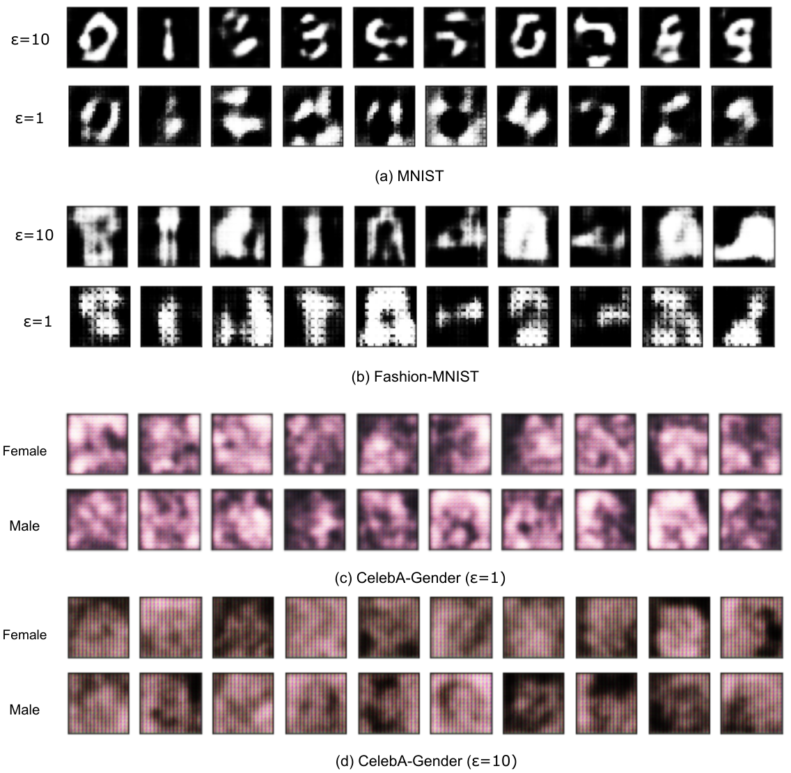
We visualize the private synthetic images for MNIST, Fashion-MNIST and CelebA, as shown in Figure 4. As expected the image has a lot of noise, since our goal is to generate data which can protect privacy and ensure high data utility in terms of training high performance models. It is interesting to see that these generated images are enough to train useful models, which lead to interesting future direction on what ML models actually learn from data.
Appendix C Experimental Details
C.1. Visual Quality Evaluation
We evaluate both Inception Score and Frechet Inception Distance for DataLens and baselines over four datasets. We present the evaluation results in Table 12(b).
For Inception Score, in our experiments, we follow GS-WGAN and use the implementation77 7 https://github.com/ChunyuanLI/MNIST_Inception_Score for Inception Score calculation with pretrained classifiers trained on real datasets (with test accuracy equal to on MNIST, Fashion-MNIST, and CelebA-Gender).
For FID, we observe it is not necessarily consistent with Inception Score (e.g., for MNIST , DataLens has better IS than G-PATE, but worse FID than G-PATE), which we think the reason is because FID is evaluated based on models trained with ImageNet which may not be suitable for evaluating datasets such as MNIST. In our experiments, we follow GS-WGAN and use the implementation88 8 https://github.com/google/compare_gan for FID calculation.
C.2. Adapting Other Gradient Compression Algorithms to DataLens
In this section, we illustrate how we adapt D2P-Fed and FetchSGD to DataLens framework.
For D2P-Fed, we replace our Algorithm 2 (TopkStoSignGrad) that uses stochastic sign compression with their method, which essentially uses k-level gradient quantization and random rotation for gradient pre-processing. The detailed algorithm is shown in Algorithm 6 and Algorithm 5.
For FetchSGD, we uses the same stochastic sign compression as we leverage sign signal as teacher voting in PATE framework. During aggregation, we use Count Sketch data structure, and use top- and unsketch operation to retrieve the aggregated gradient. The detailed algorithm is shown in Algorithm 7.
| Dataset | Metrics | Real data | DP-GAN | PATE-GAN | G-PATE | GS-WGAN | DataLens |
| MNIST | IS | 9.86 | 1.00 | 1.19 | 3.60 | 1.00 | 4.37 |
| FID | 1.04 | 470.20 | 231.54 | 153.38 | 489.75 | 186.06 | |
| Fashion-MNIST | IS | 9.01 | 1.03 | 1.69 | 3.41 | 1.00 | 3.93 |
| FID | 1.54 | 472.03 | 253.19 | 214.78 | 587.31 | 194.98 | |
| CelebA | IS | 1.88 | 1.00 | 1.15 | 1.11 | 1.00 | 1.18 |
| FID | 2.38 | 485.92 | 434.47 | 302.45 | 437.33 | 297.73 |
| Dataset | Metrics | Real data | DP-GAN | PATE-GAN | G-PATE | GS-WGAN | DataLens |
| MNIST | IS | 9.86 | 1.00 | 1.46 | 5.16 | 8.59 | 5.78 |
| FID | 1.04 | 304.86 | 253.55 | 150.62 | 58.77 | 173.50 | |
| Fashion-MNIST | IS | 9.01 | 1.05 | 2.35 | 4.33 | 5.87 | 4.58 |
| FID | 1.54 | 433.38 | 229.25 | 171.90 | 135.47 | 167.68 | |
| CelebA | IS | 1.88 | 1.00 | 1.16 | 1.12 | 1.00 | 1.42 |
| FID | 2.38 | 485.41 | 424.60 | 323.95 | 432.58 | 320.84 |
Appendix D Proofs
Proof of Theorem 7.
We have
where the last equality holds because follows the normal distribution with mean and variance , concluding the proof.
Proof of Theorem 8.
We begin by fixing . The assumption that has -Lipschitz gradient, i.e., , implies, through a well-known argument, that
Recall that Taking the expectation over the quantization and the insertion of data-privacy noise yields
where we used the Cauchy-Schwarz inequality for .
For note that
Claim 1. For and under the assumptions from Theorem 8 one has
| (4) |
Proof of Claim 1. For the ease of notation, let and . First note that, per coordinate ,
The main idea is to prove that one of these yields the main term, which would correspond to for the usual gradient descent, and for the signed gradient descent. With that in mind, let us for each define and , with and , for all . Then
To explore the above mentioned dichotomy, we now rewrite the quantity we are trying to estimate in two ways:
We start by bounding and . For we have
Therefore, for we have
| (5) |
We bound in a similar vein as in (Bernstein et al. 2018c). Note that
Let . Then . Note that
using the Cauchy-Schwarz inequality. This yields
| (6) |
We now want to prove that either or . For the sake of contradiction, suppose that
| (7) |
It is easy to see that these conditions, for imply
| (8) |
whereas for they imply
| (9) |
Let
noting that and . Moreover, since each is a partition of , we have , for all , and for all . Rewriting (8) yields
It is easy to see that this implies
| (10) |
Rewriting (9) in the similar vein yields
which together with 10 implies
which holds only if , contradicting our assumption. Therefore, either or , which proves Claim 1.
Continuing the proof of Theorem 8, we now bound by
We will now bound the RHS in two different ways. First, by expanding different cases per coordinate, it is easy to see that
by assumption. Therefore,
by the Cauchy-Schwarz inequality and the assumption .
On the other hand, since , we easily get
Combining the bounds with respect to and and adding easy analysis of different cases for scaling by yields
| (11) |
For note that
Combining bounds on and yields
Summing over all yields
which after dividing with finishes the proof of the first part.
For the moreover part, in which no quantization is performed, i.e., , for all (point-wise, not just on average), the calculation for becomes
Continuing the proof as above (summing over all and dividing by ) finishes the proof of the second part.