跳到论文正文
W Papers独立论文阅读器 arXiv:2103.10776 论文正文 计算阅读时间 · 0%
引用这篇论文根据当前论文元数据生成,正式投稿前建议核对。


License: CC BY 4.0
arXiv:2103.10776v2 [math-ph] 10 Jun 2021

The square lattice Ising model on the rectangle III:
Hankel and Toeplitz determinants

Alfred Hucht Affiliation: Faculty of Physics, University of Duisburg-Essen, 47048 Duisburg, Germany
August 11, 2026
Abstract

Based on the results obtained in [Hucht, J. Phys. A: Math. Theor. 50, 065201 (2017)], we show that the partition function of the anisotropic square lattice Ising model on the L×ML\times M rectangle, with open boundary conditions in both directions, is given by the determinant of a M/2×M/2\nicefrac{{M}}{{2}}\times\nicefrac{{M}}{{2}} Hankel matrix, that equivalently can be written as the Pfaffian of a skew-symmetric M×MM\times M Toeplitz matrix. The M−1M-1 independent matrix elements of both matrices are Fourier coefficients of a certain symbol function, which is given by the ratio of two characteristic polynomials. These polynomials are associated to the different directions of the system, encode the respective boundary conditions, and are directly related through the symmetry of the considered Ising model under exchange of the two directions. The results can be generalized to other boundary conditions and are well suited for the analysis of finite-size scaling functions in the critical scaling limit using Szegő’s theorem.

1 Introduction

The anisotropic two-dimensional Ising model (Ising25) on the L×ML\times M square lattice is one of the best investigated models in statistical mechanics. In the thermodynamic limit L,M→∞L,M\to\infty, it has a continuous phase transition, from a disordered high-temperature phase to an ordered low-temperature phase, at a critical temperature TcT_{\mathrm{c}}. After the exact solution of the periodic case by Onsager (Onsager44; Kaufman49), many authors have contributed to the knowledge about this model under various aspects, such as different boundary conditions (BCs) or surface effects (McCoyWu73; Baxter82; Abraham86).

Until some years ago, exact solutions for arbitrary temperatures were only known for systems with periodic or antiperiodic boundary conditions in at least one direction, as then a Fourier transform along this translationally invariant direction could be used to diagonalize the problem in the corresponding direction. The remaining direction could be handled afterwards with a transfer matrix method, involving a 2×22\times 2 transfer matrix, taking into account arbitrary boundary conditions, or even line disorder (McCoyWu73).

This changed in 2016, when Baxter (Baxter16; Baxter20) and Hucht (Hucht16a; Hucht16ae; Hucht16b) independently presented exact results for the Ising model on the rectangle, with open boundary conditions in both directions, expressing the partition function as M×MM\times M and M/2×M/2M/2\times M/2 determinants, respectively. While Baxter used Kaufman’s spinor method (Kaufman49) below TcT_{\mathrm{c}} and focused on the thermodynamic limit (Baxter16), where he exactly calculated the corner contributions to the free energy conjectured in (VernierJacobsen12), Hucht utilized the dimer method of Kasteleyn and McCoy & Wu (Kasteleyn61; Kasteleyn63; Fisher66; McCoyWu73; McCoyWu14), combined with Schur reductions and a block transfer matrix formulation of Molinari (Molinari08), and derived closed expressions for finite systems at arbitrary temperatures. The resulting transfer matrices directly correspond to the spinor method matrices, bridging the gap between these so far rather unrelated methods.

Near the critical temperature TcT_{\mathrm{c}}, the direction-dependent bulk correlation length of thermal fluctuations ξ∞δ​(T)\xi_{\infty}^{\delta}(T) diverges according to ξ∞δ​(T>Tc)≃ξ0δ​(T/Tc−1)−ν\xi_{\infty}^{\delta}(T\,{>}\,T_{\mathrm{c}})\simeq\xi_{0}^{\delta}(T/T_{\mathrm{c}}-1)^{-\nu}, where δ=↔,↕\delta=\,\leftrightarrow,\updownarrow denotes the directions corresponding to LL and MM, ξ0δ\xi_{0}^{\delta} are interaction-dependent metric factors, and the correlation length critical exponent is ν=1\nu=1 in the two-dimensional Ising model11 1 The relation “≃\simeq” denoted “asymptotically equal” in the respective limit, and ≡\equiv denotes a definition.. If ξ∞↔,↕(T)\xi_{\infty}^{\leftrightarrow,\updownarrow}(T) is of the order of (or larger as) the respective system size LL or MM, interesting finite-size effects such as the critical Casimir effect emerge, which describes interactions of the system boundaries mediated by long-range critical fluctuations (FisherdeGennes78; FisherAu-Yang80) in close analogy to the quantum electrodynamical Casimir effect (CasimirPolder48; Casimir48). These finite-size effects can be described (HuchtGruenebergSchmidt11) by universal finite-size scaling functions of the form Θ↕​(x↕,ρ)\Theta_{\updownarrow}(x_{\updownarrow},\rho), with temperature scaling variable x↕≡(T/Tc−1)​(M/ξ0↕)1/νx_{\updownarrow}\equiv(T/T_{\mathrm{c}}-1)(M/\xi_{0}^{\updownarrow})^{1/\nu} and generalized aspect ratio ρ≡(L/ξ0↔)/(M/ξ0↕)\rho\equiv(L/\xi_{0}^{\leftrightarrow})/(M/\xi_{0}^{\updownarrow}), that only depend on the bulk and surface universality classes of the model (Kadanoff66; Diehl97a), as well as on the BCs. They have been calculated exactly for many cases, albeit mostly in strip geometry, where the aspect ratio ρ\rho of the system goes to zero (EvansStecki94; Au-YangFisher80; BrankovDantchevTonchev00; Gambassi09a; RudnickZandiShackellAbraham10; AbrahamMaciolek10; AbrahamMaciolek13). The theoretical results from exact calculations, field theory and Monte Carlo simulations (AbrahamMaciolek10; AbrahamMaciolek13; Gambassi09a; Hasenbusch0905; Hasenbusch0907; Hasenbusch0908; Hasenbusch1005; Hasenbusch1104; Hasenbusch1205; Hucht07a; MaciolekGambassiDietrich07; RudnickZandiShackellAbraham10; VasilyevGambassiMaciolekDietrich07; VasilyevGambassiMaciolekDietrich09; HobrechtHucht14) were shown to be in excellent agreement with experiments (GarciaChan99url; GarciaChan00a; GarciaChan00b; GarciaChan02; FukutoYanoPershan05; GanshinScheidemantelGarciaChan06; HertleinHeldenGambassiDietrichBechinger08; GamMacHerNelHelBechDiet09) for various bulk and surface universality classes.

Figure 1: The anisotropic square lattice Ising model on the L×ML\times M rectangle (black), together with its dual lattice (red) and with the relevant couplings (see text). The transfer matrix 𝓣\bm{\mathrm{\mathcal{T}}} (1.6) propagates as indicated.

Directly at the critical point, exact methods or conformal field theory (Polyakov70; Cardy84; BurkhardtEisenriegler95; Cardy2006; BimonteEmigKardar13) can be used to get exact expressions for the Casimir amplitude ΔC​(ρ)\Delta_{\mathrm{C}}(\rho) for arbitrary ρ\rho. This has been done for periodic (FerdinandFisher69; LuWu01) as well as for open BCs (KlebanVassileva91; WuIzmailianGuo12). Using conformal maps, these results can be used to investigate fluctuation-induced forces between colloids in critical suspensions both in theory (SchlesenerHankeDietrich03; KHD09; TrKoGamHarDiet09; GambassiDietrich10; TrZvGamVogtHarBechDiet11; Hasenbusch13; LTHD14; HobrechtHucht15a; ETBEvRD15) and experiment (BrunnerDobnikar04; SoykaZvyaHertHeldBech08; BonnOtwiSacaGuoWegSchall09; ZAB11; GZS12; GZTS12; DVNBS13; NguyenFaHuWeSch13; TasiosDijkstra17). At arbitrary aspect ratios and temperatures, however, the finite-size scaling functions must be derived from the exact solution of the finite system with the correct BCs. For the Ising model, this has been done only in a few cases, namely for the torus with periodic BCs in both directions (HuchtGruenebergSchmidt11; HobrechtHucht16a; HobrechtHucht18a), for the cylinder with open or fixed at the boundaries in one direction (HobrechtHucht16a; HobrechtHucht18b), and for the open rectangle considered here (Hucht16b).

In this work, the calculations of (Hucht16a) are substantially simplified by (i) the use of elliptic functions (Baxter82), (ii) a simplified normalization of the eigenvectors of the relevant M×MM\times M transfer matrices, (iii) a transformation to Hankel and Toeplitz matrices, and (iv) a representation of the sums over transfer matrix eigenvalues through a complex contour integral, having (v) a remarkably simple integrand given by the ratio of two very simple characteristic polynomials, each representing one direction of the two-dimensional Ising model. The preceding publication (Hucht16a) will be denoted I in the following.

1.1 The model

This work focuses on the anisotropic square lattice Ising model on the L×ML\times M open rectangle, shown in figure 1. Our aim is to calculate the partition function

Z=tr⁡exp⁡(𝒦↔​∑ℓ=1L−1∑m=1Mσℓ,m​σℓ+1,m+𝒦↕​∑ℓ=1L∑m=1M−1σℓ,m​σℓ,m+1),Z=\Tr\exp\left(\mathcal{K}^{\leftrightarrow}\sum_{\ell=1}^{L-1}\sum_{m=1}^{M}\sigma_{\ell,m}\sigma_{\ell+1,m}+\mathcal{K}^{\updownarrow}\sum_{\ell=1}^{L}\sum_{m=1}^{M-1}\sigma_{\ell,m}\sigma_{\ell,m+1}\right), (1.1)

with reduced couplings 𝒦δ=β​Jδ\mathcal{K}^{\delta}=\beta J^{\delta} in direction δ=↔,↕\delta=\,\leftrightarrow,\updownarrow, where the trace is over all 2L​M2^{LM} configurations of the L​MLM spins σℓ,m=±1\sigma_{\ell,m}=\pm 1. We assume open BCs both in horizontal (LL) and in vertical (MM) directions, and we assume even MM. The starting point of this work is the matrix product representation (I.29) of the well known Pfaffian representation by Kasteleyn, McCoy & Wu (Kasteleyn63; McCoyWu73), derived in (Hucht16a) using a Schur reduction as well as a block transfer matrix formula by Molinari (Molinari08). We follow the notation of (Hucht16a), with a few clarifying minor modifications. Therefore, we define the dual

a∗≡1−a1+aa^{*}\equiv\frac{1-a}{1+a} (1.2)

of some quantity aa, as well as the quite useful abbreviations22 2 Subscripts a±a_{\pm} are consequently used in this manner, while superscripts a±a^{\pm} may have different meanings.

a±≡a±a−12a_{\pm}\equiv\frac{a\pm a^{-1}}{2} (1.3)

introduced in (I.20), fulfilling (a∗)∗=a=a++a−(a^{*})^{*}=a=a_{+}+a_{-}. The reduced couplings 𝒦δ\mathcal{K}^{\delta} are rewritten using the weights zz and tt according to

z≡tanh⁡𝒦↔,t≡(tanh⁡𝒦↕)∗=e−2​𝒦↕.z\equiv\tanh\mathcal{K}^{\leftrightarrow},\qquad t\equiv(\tanh\mathcal{K}^{\updownarrow})^{*}=\mathrm{e}^{-2\mathcal{K}^{\updownarrow}}. (1.4)

The partition function ZZ of the considered anisotropic Ising model with open BCs in both directions is invariant under exchange of the two directions ↔\leftrightarrow and ↕\updownarrow, where both the system dimensions and the coupling constants are exchanged according to the swap transformation

𝒮:(L,M,𝒦↔,𝒦↕)↦𝒮⁡[(L,M,𝒦↔,𝒦↕)]=(M,L,𝒦↕,𝒦↔),\mathcal{S}:(L,M;\mathcal{K}^{\leftrightarrow},\mathcal{K}^{\updownarrow})\mapsto\mathcal{S}[(L,M;\mathcal{K}^{\leftrightarrow},\mathcal{K}^{\updownarrow})]=(M,L;\mathcal{K}^{\updownarrow},\mathcal{K}^{\leftrightarrow}), (1.5)

such that Z=𝒮⁡[Z]Z=\mathcal{S}[Z]. The swap transformation is a involution, as 𝒮⁡[𝒮⁡[a]]=a\mathcal{S}[\mathcal{S}[a]]=a. We now summarize the required results from reference (Hucht16a).

1.2 Starting point

In equations (27-29) of (Hucht16a) we showed that the square of the partition function (1.1) is proportional to the determinant of a matrix product of the form ⟨𝐞2|𝓣2L|𝐞2⟩\langle\bm{\mathrm{e}}_{2}|\bm{\mathrm{\mathcal{T}}}_{2}^{L}|\bm{\mathrm{e}}_{2}\rangle, with real hyperbolic 2×22\times 2 block transfer matrix 𝓣2\bm{\mathrm{\mathcal{T}}}_{\!2} propagating in horizontal direction. In this work, we will use a “Wick rotated” version of 𝓣2\bm{\mathrm{\mathcal{T}}}_{\!2} according to33 3 𝐀⊤\bm{\mathrm{A}}\negmedspace^{\top} and 𝐀†\bm{\mathrm{A}}^{\dagger} denote the transpose and the conjugate transpose of 𝐀\bm{\mathrm{A}}, respectively. 𝓣≡𝓘​𝓣2​𝓘†,\bm{\mathrm{\mathcal{T}}}\equiv\bm{\mathrm{\mathcal{I}}}\,\bm{\mathrm{\mathcal{T}}}_{\!2}\,\bm{\mathrm{\mathcal{I}}}^{\dagger}, with matrix 𝓘≡(100i)⊗𝟏\bm{\mathrm{\mathcal{I}}}\equiv(\begin{smallmatrix}1&0\\ 0&\mathrm{i}\end{smallmatrix})\otimes\bm{\mathrm{1}}, leading to the complex orthogonal block transfer matrix

𝓣≡[𝐓+−i​𝐓−i​𝐓−𝐓+],\bm{\mathrm{\mathcal{T}}}\equiv\begin{bmatrix}\bm{\mathrm{T}}_{+}&-\mathrm{i}\bm{\mathrm{T}}_{-}\\ \,\mathrm{i}\bm{\mathrm{T}}_{-}&\bm{\mathrm{T}}_{+}\end{bmatrix}, (1.6)

which fulfills 𝓣−1=𝓣⊤\bm{\mathrm{\mathcal{T}}}^{-1}=\bm{\mathrm{\mathcal{T}}}^{\top}. Note that 𝓣\bm{\mathrm{\mathcal{T}}} is not unitary. The two real symmetric M×MM\times M matrices 𝐓±\bm{\mathrm{T}}_{\pm} were given in (I.30) and can be simplified to

𝐓+\displaystyle\bm{\mathrm{T}}_{+} =−t−​z−2​(2+t∗z∗112⋱⋱⋱⋱⋱2112+t∗​z∗)⏟𝐂+(t+​z++t−​z−)​𝟏,\displaystyle=-\frac{t_{-}z_{-}}{2}{\,\,\underbrace{\!\!\begin{pmatrix}2{+}\frac{t^{*}}{z^{*}}&1\\ 1&2&\ddots\\ &\ddots&\ddots&\ddots\\ &&\ddots&2&1\\ &&&1&2{+}t^{*}z^{*}\end{pmatrix}\!\!}_{{\textstyle\bm{\mathrm{C}}}}}\,\,+(t_{+}z_{+}+t_{-}z_{-})\bm{\mathrm{1}}, (1.7a)
𝐓−\displaystyle\bm{\mathrm{T}}_{-} =−t−​z−2​(z∗−1t∗⋰−2​t∗+1z∗⋰⋰⋰z∗−2​t∗+⋰−1t∗1z∗),\displaystyle=-\frac{t_{-}z_{-}}{2}{\begin{pmatrix}&&&z^{*}&-\frac{1}{t^{*}}\\ &&\iddots&-2{t^{*}}_{\!+}&\frac{1}{z^{*}}\\ &\iddots&\iddots&\iddots\\ z^{*}&-2{t^{*}}_{\!+}&\iddots\\ -\frac{1}{t^{*}}&\frac{1}{z^{*}}\end{pmatrix}}, (1.7b)

using the dual couplings z∗z^{*} and t∗t^{*} (the matrix 𝐂\bm{\mathrm{C}} will be utilized later). They are related via the transfer matrix 𝐓=𝐓++𝐓−\bm{\mathrm{T}}=\bm{\mathrm{T}}_{+}+\bm{\mathrm{T}}_{-} according to (1.3),

𝐓±=12(𝐓±𝐓−1)⇔𝐓±1=𝐓+±𝐓−,\bm{\mathrm{T}}_{\pm}=\tfrac{1}{2}\left(\bm{\mathrm{T}}\pm\bm{\mathrm{T}}^{-1}\right)\quad\Leftrightarrow\quad\bm{\mathrm{T}}^{\pm 1}=\bm{\mathrm{T}}_{+}\pm\bm{\mathrm{T}}_{-}, (1.8)

from which directly follows that 𝓣\bm{\mathrm{\mathcal{T}}} can be block diagonalized through a rotation by π/4\pi/4,

𝓡π4​𝓘†​𝓣​𝓘​𝓡−π4=[𝐓𝟎𝟎𝐓−1],\bm{\mathrm{\mathcal{R}}}_{\frac{\pi}{4}}\bm{\mathrm{\mathcal{I}}}^{\dagger}\bm{\mathrm{\mathcal{T}}}\,\bm{\mathrm{\mathcal{I}}}\,\bm{\mathrm{\mathcal{R}}}_{-\frac{\pi}{4}}=\begin{bmatrix}\bm{\mathrm{T}}&\bm{\mathrm{0}}\\ \bm{\mathrm{0}}&\bm{\mathrm{T}}^{-1}\end{bmatrix}, (1.9)

with block rotation matrix 𝓡θ≡(cos⁡θsin⁡θ−sin⁡θcos⁡θ)⊗𝟏\bm{\mathrm{\mathcal{R}}}_{\theta}\equiv(\begin{smallmatrix}\cos\theta&\sin\theta\\ -\sin\theta&\cos\theta\end{smallmatrix})\otimes\bm{\mathrm{1}}, for details see chapter V in (Hucht16a). The open BCs in horizontal direction are represented through the boundary state

|𝐞o⟩≡12​|𝟏i​𝐒⟩,⟨𝐞o|𝐞o⟩=𝟏,|\bm{\mathrm{e}}_{\mathrm{o}}\rangle\equiv\frac{1}{\sqrt{2}}|\begin{array}[]{cc}\bm{\mathrm{1}}&\mathrm{i}\bm{\mathrm{S}}\end{array}\rangle,\qquad\langle\bm{\mathrm{e}}_{\mathrm{o}}|\bm{\mathrm{e}}_{\mathrm{o}}\rangle=\bm{\mathrm{1}}, (1.10)

where |𝐞o⟩|\bm{\mathrm{e}}_{\mathrm{o}}\rangle is a two element block vector, with the M×MM\times M matrices

𝟏≡\displaystyle\bm{\mathrm{1}}\equiv (1⋱1),\displaystyle\left(\begin{array}[]{ccc}1\\ &\;\;\ddots\\ &&1\end{array}\right), 𝐒≡\displaystyle\bm{\mathrm{S}}\equiv (1⋰1).\displaystyle\left(\begin{array}[]{ccc}&&1\\ &\;\;\iddots\\ 1\end{array}\right).

Together with the constant

Z0≡(1−z2)M2​(2−z−)L​M2,Z_{0}\equiv(1-z^{2})^{\frac{M}{2}}\left(\frac{2}{-z_{-}}\right)^{\negmedspace\frac{LM}{2}}\!, (1.17)

the square of the partition function (1.1) then reads

Z2=Z02​det⟨𝐞o|𝓣L|𝐞o⟩,Z^{2}=Z_{0}^{2}\det\langle\bm{\mathrm{e}}_{\mathrm{o}}|\bm{\mathrm{\mathcal{T}}}^{L}|\bm{\mathrm{e}}_{\mathrm{o}}\rangle, (1.18)

see also (Baxter16, (2.35)). Defining the projectors

𝐒±≡12​(𝟏±𝐒),\bm{\mathrm{S}}^{\pm}\equiv\frac{1}{2}\left(\bm{\mathrm{1}}\pm\bm{\mathrm{S}}\right), (1.19)

the argument of the determinant in (1.18) becomes

⟨𝐞o|𝓣L|𝐞o⟩\displaystyle\langle\bm{\mathrm{e}}_{\mathrm{o}}|\bm{\mathrm{\mathcal{T}}}^{L}|\bm{\mathrm{e}}_{\mathrm{o}}\rangle =⟨𝐒+i​𝐒−|[𝐓L𝟎𝟎𝐓−L]|𝐒+i​𝐒−⟩\displaystyle=\langle\begin{array}[]{cc}\bm{\mathrm{S}}^{+}&\mathrm{i}\bm{\mathrm{S}}^{-}\end{array}|\begin{bmatrix}\bm{\mathrm{T}}{}^{L}&\bm{\mathrm{0}}\\ \bm{\mathrm{0}}&\bm{\mathrm{T}}{}^{-L}\end{bmatrix}|\begin{array}[]{cc}\bm{\mathrm{S}}^{+}&\mathrm{i}\bm{\mathrm{S}}^{-}\end{array}\rangle
=𝐒+​𝐓​𝐒+L+𝐒−​𝐓​𝐒−−L=𝐌⊤​𝐌,\displaystyle=\bm{\mathrm{S}}^{+}\,\bm{\mathrm{T}}{}^{L}\,\bm{\mathrm{S}}^{+}+\bm{\mathrm{S}}^{-}\,\bm{\mathrm{T}}{}^{-L}\,\bm{\mathrm{S}}^{-}=\bm{\mathrm{M^{\top}}}\bm{\mathrm{M}}, (1.20c)

with the matrix

𝐌≡𝐱(𝐓L/2𝐒++𝐓−L/2𝐒−),\bm{\mathrm{M}}\equiv\bm{\mathrm{x}}\big(\bm{\mathrm{T}}^{L/2}\,\bm{\mathrm{S}}^{+}+\bm{\mathrm{T}}^{-L/2}\,\bm{\mathrm{S}}^{-}\big), (1.21)

as 𝐒+​𝐒−=𝟎\bm{\mathrm{\bm{\mathrm{S}}^{+}\bm{\mathrm{S}}^{-}=\bm{\mathrm{0}}}}. In the following we will determine the eigenvalues λμ,λ±,μ\lambda_{\mu},\lambda_{\pm,\mu} and common eigenvectors x→μ=(𝐱)μ\vec{x}_{\mu}=(\bm{\mathrm{x}})_{\mu} of 𝐓\bm{\mathrm{T}} and 𝐓±\bm{\mathrm{T}}_{\pm}, which fulfill

𝐓​x→μ\displaystyle\bm{\mathrm{T}}\,\vec{x}_{\mu} =λμ​x→μ,\displaystyle=\lambda_{\mu}\vec{x}_{\mu}, 𝐓±​x→μ\displaystyle\bm{\mathrm{T}}_{\pm}\vec{x}_{\mu} =λ±,μ​x→μ,\displaystyle=\lambda_{\pm,\mu}\vec{x}_{\mu}, (1.22)

where μ=1,…,M\mu=1,\ldots,M.

1.3 The Onsager dispersion relation

The next step in the calculation of the partition function (1.1) is the determination of the eigenvalues λ+,μ\lambda_{+,\mu} as zeroes of the characteristic polynomial (CP) of the tridiagonal matrix 𝐓+\bm{\mathrm{T}}_{+} from (1.7a), which will lead to the Onsager dispersion relation. As we will discuss several characteristic polynomials (CPs) in the following, we first define the CP P𝒂​(x)P_{\boldsymbol{a}}(x) of an arbitrary M×MM\times M matrix 𝐀\bm{\mathrm{A}}, with eigenvalues (𝒂)μ=aμ∈ℂ(\boldsymbol{a})_{\mu}=a_{\mu}\in\mathbb{C}, to be

P𝒂​(x)≡det(x​𝟏−𝐀)=∏μ=1M(x−aμ),P_{\boldsymbol{a}}(x)\equiv\det(x\bm{\mathrm{1}}-\bm{\mathrm{A}})=\prod_{\mu=1}^{M}(x-a_{\mu}), (1.23)

such that P𝒂​(x)P_{\boldsymbol{a}}(x) is a polynomial of degree MM in the indeterminate x∈ℂx\in\mathbb{C}.

Using the well known recursion formula for tridiagonal matrices (see, e.g., (Molinari08)), in (Hucht16a) we derived44 4 The sign change in the definition w.r.t. (I.9) has no effect for even MM.

P𝝀+​(λ+)\displaystyle P_{\boldsymbol{\lambda_{+}}}(\lambda_{+}) =det(λ+​𝟏−𝐓+)=∏μ=1M(λ+−λ+,μ)\displaystyle=\det(\lambda_{+}\bm{\mathrm{1}}-\bm{\mathrm{T}}_{+})=\prod_{\mu=1}^{M}(\lambda_{+}-\lambda_{+,\mu}) (1.24a)
=(t−​z−2)M​⟨1/z∗−t∗|𝐐M|z∗t∗⟩,\displaystyle=\left(\frac{t_{-}z_{-}}{2}\right)^{\negmedspace M}\langle\begin{array}[]{cc}1/z^{*}&-t^{*}\end{array}|\,\bm{\mathrm{Q}}^{M}\,|\begin{array}[]{cc}z^{*}&t^{*}\end{array}\rangle,

where λ+∈ℂ\lambda_{+}\in\mathbb{C}. We point out the obvious similarity between equations (1.18) and (1.24), which will become clearer later. The vertically propagating 2×22\times 2 transfer matrix

𝐐≡(2​t+​z+−λ+t−​z−−110)=(2​ζ+−110)=(2​cos⁡φ−110)\bm{\mathrm{Q}}\equiv\begin{pmatrix}2\frac{t_{+}z_{+}-\lambda_{+}}{t_{-}z_{-}}&-1\\ 1&0\end{pmatrix}=\begin{pmatrix}2\zeta_{+}&-1\\ 1&0\end{pmatrix}=\begin{pmatrix}2\cos\varphi\,&-1\\ 1&0\end{pmatrix} (1.25)

has the eigenvalues ζ±1\zeta^{\pm 1} with modulus one55 5 ζ±1\zeta^{\pm 1} were denoted q±q^{\pm} in (I.42)., such that the nn-th power of 𝐐\bm{\mathrm{Q}} reads

𝐐n=1sin⁡φ​(sin⁡([n+1]​φ)−sin⁡(n​φ)sin⁡(n​φ)−sin⁡([n−1]​φ)).\bm{\mathrm{Q}}^{n}=\frac{1}{\sin\varphi}\begin{pmatrix}\sin([n+1]\varphi)&-\sin(n\varphi)\\ \sin(n\varphi)&-\sin([n-1]\varphi)\end{pmatrix}. (1.26)

Here and in the following, we express the horizontal and vertical eigenvalues (λ,ζ)(\lambda,\zeta) through the introduced angles (γ,φ)(\gamma,\varphi) according to

λ\displaystyle\lambda =eγ,\displaystyle=\mathrm{e}^{\gamma}, λ+\displaystyle\lambda_{+} =cosh⁡γ,\displaystyle=\cosh\gamma, λ−\displaystyle\lambda_{-} =sinh⁡γ,\displaystyle=\sinh\gamma, (1.27a)
ζ\displaystyle\zeta =ei​φ,\displaystyle=\mathrm{e}^{\mathrm{i}\varphi}, ζ+\displaystyle\zeta_{+} =cos⁡φ,\displaystyle=\cos\varphi, ζ−\displaystyle\zeta_{-} =i​sin⁡φ.\displaystyle=\mathrm{i}\sin\varphi. (1.27b)

Equation (1.25) is the point in the calculation where the famous Onsager dispersion relation

λ++t−z−ζ+=t+z+⇔coshγ+t−z−cosφ=t+z+\lambda_{+}+t_{-}z_{-}\zeta_{+}=t_{+}z_{+}\qquad\Leftrightarrow\qquad\cosh\gamma+t_{-}z_{-}\cos\varphi=t_{+}z_{+} (1.28)

between the eigenvalues λ\lambda and ζ\zeta enters the stage, which plays the key role in the exact solution of the square lattice Ising model (Onsager44). It relates the two “good” variables λ\lambda and ζ\zeta for propagation in ↔\leftrightarrow (LL) and ↕\updownarrow (MM) direction, respectively. As pointed out by Baxter (Baxter82, chap. 15.10), a parametrization of relation (1.28) using elliptic functions considerably simplifies the analysis. This parametrization is introduced in the next chapter, and we return to the characteristic polynomials in chapter 3.1.

2 Elliptic parametrization

The key idea behind the elliptic parametrization of the Onsager dispersion relation (1.28) is (i) to substitute the coupling constants (z,t)(z,t) through new constants (k,η)(k,\eta), where kk is temperature-like and η\eta encodes the coupling anisotropy, and (ii) to introduce a complex variable uu that simultaneously parametrizes the quantities ζ=ζ⁡(u)\zeta=\zeta(u) and λ=λ⁡(u)\lambda=\lambda(u) in such a way that (1.28) is always fulfilled66 6 Imagine the simpler case of a circle x2+y2=r2x^{2}+y^{2}=r^{2} being trigonometrically parametrized, with x⁡(u)=r​cos⁡ux(u)=r\cos u, y⁡(u)=r​sin⁡uy(u)=r\sin u and complex parameter uu.. We recapitulate the parametrization of (1.28) through the Jacobi elliptic functions sn⁡(u,k)\Jsn(u,k), cn⁡(u,k)\Jcn(u,k) and dn⁡(u,k)\Jdn(u,k) (Lawden89; NIST; NIST:DLMF), with elliptic modulus kk, by first defining the Jacobi amplitude

ϕ≡am⁡(u,k)\phi\equiv\Jam(u,k) (2.1)

as the inverse function of the elliptic integral of the first kind

u=F(ϕ,k)≡∫0ϕ(1−k2sin2θ)−1/2dθ,u=F(\phi,k)\equiv\int_{0}^{\phi}(1-k^{2}\sin^{2}\theta)^{-1/2}\mathrm{d}\theta, (2.2)

for {ϕ,u,k}∈ℝ.\{\phi,u,k\}\in\mathbb{R}. Consequently, the Jacobi elliptic functions are given by

sn⁡(u,k)≡sin⁡ϕ,cn⁡(u,k)≡cos⁡ϕ,dn⁡(u,k)≡∂ϕ∂u=±1−k2​sin2⁡ϕ,\Jsn(u,k)\equiv\sin\phi,\qquad\Jcn(u,k)\equiv\cos\phi,\qquad\Jdn(u,k)\equiv\frac{\partial\phi}{\partial u}=\pm\sqrt{1-k^{2}\sin^{2}\phi}, (2.3)

and fulfill the sum of squares identities

sn2⁡(u,k)+cn2⁡(u,k)=k2​sn2⁡(u,k)+dn2⁡(u,k)=1.\Jsn^{2}(u,k)+\Jcn^{2}(u,k)=k^{2}\Jsn^{2}(u,k)+\Jdn^{2}(u,k)=1. (2.4)

As common, we suppress the modulus kk if possible and write, e. g., sn⁡u\Jsn u instead of sn⁡(u,k)\Jsn(u,k). We follow Glashier’s notation (NIST:DLMF, (22.2.10)) and define all sixteen Jacobi elliptic functions

pq​u≡pr​uqr​u=1qp​u,wherep,q,r∈{s,c,d,n},\mathrm{pq}\,u\equiv\frac{\mathrm{pr}\,u}{\mathrm{qr}\,u}=\frac{1}{\mathrm{qp}\,u},\qquad\mathrm{where}\qquad\mathrm{p},\mathrm{q},\mathrm{r}\in\{\mathrm{s},\mathrm{c},\mathrm{d},\mathrm{n}\}, (2.5)

including the four trivial ones, ss⁡u=cc⁡u=dd⁡u=nn⁡u=1\Jss u=\Jcc u=\Jdd u=\Jnn u=1.

The Jacobi elliptic functions are double periodic and meromorphic in the complex uu-plane, that is they are analytic up to simple poles. The common quarter-periodicity rectangle has the corners

{us,uc,ud,un}≡{0,K,K+i​K′,i​K′},\{u_{\mathrm{s}},u_{\mathrm{c}},u_{\mathrm{d}},u_{\mathrm{n}}\}\equiv\{0,K,K+\mathrm{i}K^{\prime},\mathrm{i}K^{\prime}\}, (2.6)

see figure 2, where we utilized the graphical interpretation from (NIST:DLMF, (22.4)) and associate the denomination {s,c,d,n}\{\mathrm{s},\mathrm{c},\mathrm{d},\mathrm{n}\} with the four vertices of the quarter-periodicity rectangle. Eventually, the quarter periods KK and K′K^{\prime} are the complete elliptic integrals of the first kind,

K\displaystyle K ≡F⁡(π2,k),\displaystyle\equiv F\big(\tfrac{\pi}{2},k\big), K′\displaystyle K^{\prime} ≡F⁡(π2,k′),\displaystyle\equiv F\big(\tfrac{\pi}{2},k^{\prime}\big), (2.7)

cf. (2.2), with complementary modulus k′k^{\prime} fulfilling k2+k′2=1k^{2}+k^{\prime 2}=1. This elliptic parametrization will lead to substantial simplifications of the results from (Hucht16a), as it firstly eliminates the sign ambiguities of the square roots and secondly introduces certain functions of the parameter uu that substantially simplify the expressions.

2.1 Coupling constants parametrization

There are several possible ways to setup an elliptic parametrization of the Onsager dispersion relation (1.28): one could set k=k^≡z−/t−k=\hat{k}\equiv z_{-}/t_{-} such that 0≤k^<10\leq\hat{k}<1 holds in the ordered phase. This choice is usually used in the literature (IorgovLisovyy11; Baxter16). However, we will argue that many expressions become considerably simpler if we instead use the modulus

k≡t−z−,k\equiv\frac{t_{-}}{z_{-}}, (2.8)

being the reciprocal of k^\hat{k}. It obeys 0≤k<10\leq k<1 in the disordered phase T>TcT>T_{\mathrm{c}} and k>1k>1 in the ordered phase T<TcT<T_{\mathrm{c}}, similar to the reduced inverse temperature β/βc\beta/\beta_{\mathrm{c}}. Note that KK becomes complex for k>1k>1, and we can replace it with its real part, K↦ℜ⁡(K)=K+i​K′K\mapsto\Re(K)=K+\mathrm{i}K^{\prime}, in the complex analysis in order to keep an un-tilted quarter-periodicity rectangle.

The anisotropy parameter η\eta can be introduced in several ways, too. We choose the definition

sn⁡(2​η)≡1i​t−,\Jsn(2\eta)\equiv\frac{1}{\mathrm{i}t_{-}}, (2.9)

such that η\eta is a purely imaginary point in the uu-plane, with 0≤ℑ⁡(η)≤K′/20\leq\Im(\eta)\leq K^{\prime}/2. This leads to the identities

t\displaystyle t =sn⁡η​dn⁡ηi​cn⁡η,\displaystyle=\frac{\Jsn\eta\Jdn\eta}{\mathrm{i}\Jcn\eta}, t+\displaystyle t_{+} =i​cs⁡(2​η),\displaystyle=\mathrm{i}\Jcs(2\eta), t−\displaystyle t_{-} =1i​ns⁡(2​η),\displaystyle=\frac{1}{\mathrm{i}}\Jns(2\eta), (2.10a)
z\displaystyle z =k​sn⁡η​cn⁡ηi​dn⁡η,\displaystyle=k\frac{\Jsn\eta\Jcn\eta}{\mathrm{i}\Jdn\eta}, z+\displaystyle z_{+} =ik​ds⁡(2​η),\displaystyle=\frac{\mathrm{i}}{k}\Jds(2\eta), z−\displaystyle z_{-} =1i​k​ns⁡(2​η).\displaystyle=\frac{1}{\mathrm{i}k}\Jns(2\eta). (2.10b)

For the dual couplings we find the corresponding expressions

t∗+\displaystyle{t^{*}}_{\!+} =−t+t−=cn⁡(2​η),\displaystyle=-\frac{t_{+}}{t_{-}}=\Jcn(2\eta), t∗−\displaystyle{t^{*}}_{\!-} =1t−=i​sn⁡(2​η),\displaystyle=\frac{1}{t_{-}}=\mathrm{i}\Jsn(2\eta), (2.11a)
z∗+\displaystyle{z^{*}}_{\!+} =−z+z−=dn⁡(2​η),\displaystyle=-\frac{z_{+}}{z_{-}}=\Jdn(2\eta), z∗−\displaystyle{z^{*}}_{\!-} =1z−=i​k​sn⁡(2​η),\displaystyle=\frac{1}{z_{-}}=\mathrm{i}k\Jsn(2\eta), (2.11b)

which implies that we can express tt, zz, t∗t^{*} and z∗z^{*} through the Jacobi amplitude (2.1),

t∗\displaystyle t^{*} =ei​am⁡(2​η),\displaystyle=\mathrm{e}^{\mathrm{i}\Jam(2\eta)}, t\displaystyle t =−i​tan⁡[12​am⁡(2​η)],\displaystyle=-\mathrm{i}\tan\!\left[{\textstyle\frac{1}{2}}\Jam(2\eta)\right], (2.12a)
z\displaystyle z =ei​am⁡(2​η~),\displaystyle=\mathrm{e}^{\mathrm{i}\Jam(2\tilde{\eta})}, z∗\displaystyle z^{*} =−i​tan⁡[12​am⁡(2​η~)],\displaystyle=-\mathrm{i}\tan\!\text{$\left[{\textstyle\frac{1}{2}}\Jam(2\tilde{\eta})\right]$}, (2.12b)

where u~\tilde{u} denotes the swap transform (1.5) of a point uu in the complex uu-plane,

u↦u~≡𝒮⁡(u)=12​i​K′−u.u\mapsto\tilde{u}\equiv\mathcal{S}(u)={\textstyle\frac{1}{2}}\mathrm{i}K^{\prime}-u. (2.13)

From (2.2) and the t∗t^{*} identity (2.12a) we conclude that

2​η=F⁡(−i​log⁡t∗,k)=i​K′−F⁡(−i​log⁡z,k).2\eta=F(-\mathrm{i}\log t^{*},k)=\mathrm{i}K^{\prime}-F(-\mathrm{i}\log z,k). (2.14)

Note that in the isotropic case t∗=zt^{*}=z the point η\eta lies symmetrically at

ηiso≡14​i​K′=η~iso,\eta_{\mathrm{iso}}\equiv{\textstyle\frac{1}{4}}\mathrm{i}K^{\prime}=\tilde{\eta}_{\mathrm{iso}}, (2.15)

as 𝒮⁡(ηiso)=ηiso\mathcal{S}(\eta_{\mathrm{iso}})=\eta_{\mathrm{iso}}. Therefore, the transformation (2.13) is a point reflection of the complex uu-plane at the point ηiso\eta_{\mathrm{iso}}.

2.2 Eigenvalues parametrization

The relation of the eigenvalues λ\lambda and ζ\zeta (1.27) to uu is also ambiguous. We follow the literature (Baxter82; IorgovLisovyy11; Baxter16) and define

1λ​ζ±1=e−γ±i​φ2≡k​sn⁡(u∓η),\frac{1}{\sqrt{\lambda\zeta^{\pm 1}}}=\mathrm{e}^{-\frac{\gamma\pm\mathrm{i}\varphi}{2}}\equiv\sqrt{k}\Jsn(u\mp\eta), (2.16)

such that

λ\displaystyle\lambda =eγ=1k​sn⁡(u+η)​sn​(u−η),\displaystyle=\mathrm{e}^{\gamma}=\frac{1}{k\Jsn(u+\eta)\Jsn(u-\eta)}, ζ\displaystyle\zeta =ei​φ=sn⁡(u+η)sn⁡(u−η).\displaystyle=\mathrm{e}^{\mathrm{i}\varphi}=\frac{\Jsn(u+\eta)}{\Jsn(u-\eta)}. (2.17)

The real and positive eigenvalues λμ\lambda_{\mu} correspond to values uμu_{\mu} on the real axis (for λμ>1\lambda_{\mu}>1) as well as on the line ℑ⁡(uμ)=i​K′\Im(u_{\mu})=\mathrm{i}K^{\prime} (for λμ<1\lambda_{\mu}<1). With this definition of λ\lambda, the constants upu_{\mathrm{p}} and λp\lambda_{\mathrm{p}} from (2.6) and (A.1) fulfill λp=λ⁡(up)\lambda_{\mathrm{p}}=\lambda(u_{\mathrm{p}}) and represent the upper and lower bound of the spectrum of 𝐓\bm{\mathrm{T}} and 𝐓−1\bm{\mathrm{T}}^{-1} both above and below TcT_{\mathrm{c}}. In appendix A we give a subset of the large number of identities which can be derived using elliptic functions identities (Lawden89; NIST:DLMF). Especially, we see from (A.11) that the eigenvalues λ\lambda and ζ\zeta are exchanged under the transformation 𝒮\mathcal{S} according to 𝒮⁡[(λ,ζ)]=(ζ,λ)\mathcal{S}[(\lambda,\zeta)]=(\zeta,\lambda).

Figure 2: Structure of the complex elliptic uu-plane for M=4M=4, paramagnetic temperature k=0.95k=0.95, and anisotropy η=34​ηiso\eta=\frac{3}{4}\eta_{\mathrm{iso}}. The eigenvalues λμ\lambda_{\mu} translate to the points uμu_{\mu} (red), while the swap-transformed points u~μ\tilde{u}_{\mu} (blue) represent the eigenvalues ζμ\zeta_{\mu} and lie point-symmetric w.r.t. the point ηiso\eta_{\mathrm{iso}} (green) from (2.15). The corners (2.6) of the quarter-periodicity rectangle are shown in black. The additional eigenvalues λμ−1\lambda_{\mu}^{-1} at positions uˇμ≡uμ+i​K′\check{u}_{\mu}\equiv u_{\mu}+\mathrm{i}K^{\prime} (C.5) and the corresponding eigenvalues ζμ−1\zeta_{\mu}^{-1} are shown in light colors.

Besides the corners of the quarter-periodicity rectangle (2.6), and the eigenvalues uμu_{\mu}, where the CP (1.24) is zero, there are four other important points in the complex uu-plane, namely the positions of the simple poles and simple zeroes of λ⁡(u)\lambda(u) and ζ⁡(u)\zeta(u). Because the Jacobi sn⁡u\Jsn u has a simple zero at u=0u=0 and a simple pole at u=i​K′u=\mathrm{i}K^{\prime}, we find

uλ→∞,ζ→∞\displaystyle u_{\lambda\to\infty,\zeta\to\infty} =+η,\displaystyle=+\eta, uλ→0,ζ→∞\displaystyle u_{\lambda\to 0,\zeta\to\infty} =+i​K′−η,\displaystyle=+\mathrm{i}K^{\prime}-\eta, (2.18a)
uλ→∞,ζ→0\displaystyle u_{\lambda\to\infty,\zeta\to 0} =−η,\displaystyle=-\eta, uλ→0,ζ→0\displaystyle u_{\lambda\to 0,\zeta\to 0} =−i​K′+η.\displaystyle=-\mathrm{i}K^{\prime}+\eta. (2.18b)

These four points will be used later in the analysis of the complex structure of the relevant integrals.

While KK and K′K^{\prime} are the quarter periods of the Jacobi elliptic functions (2.3), all relevant parameters and variables of the considered system, such as t,z,λ,ζt,z,\lambda,\zeta, can be written as meromorphic functions of 2​u2u and 2​η2\eta, see (2.12), (A.16), and (A.17). They are therefore double periodic functions with quarter periods K/2K/2 and K′/2K^{\prime}/2 and half periods KK and K′K^{\prime}, and can be depicted on the periodicity rectangle going from −K−i​K′-K-\mathrm{i}K^{\prime} to K+i​K′K+\mathrm{i}K^{\prime}, as shown in figure 2.

Finally, we remark that the CP zeroes show up in pairs (uμ,−u¯μ)(u_{\mu},-\bar{u}_{\mu}), lying symmetrically with respect to the imaginary axis, see figure 2. The reason for this symmetry is the meromorphicity of the Jacobi elliptic functions, and consequently of λ⁡(u)\lambda(u) and ζ⁡(u)\zeta(u) from (2.17), in combination with the fact that both λ\lambda and ζ\zeta are real for purely imaginary uu. Therefore, λ\lambda and ζ\zeta transform according to f⁡(u)=f⁡(−u¯)¯f(u)=\overline{f(-\bar{u})} under conjugation. This symmetry is sometimes called para-even in the literature, and −u¯-\bar{u} is denoted the para-conjugate of uu (BultheelBarel, 6.29). We could restore the usual symmetry along the real axis f⁡(u)=f⁡(u¯)¯f(u)=\overline{f(\bar{u})}, valid for meromorphic functions f⁡(u)f(u) that are real for real uu, by rotating the complex plane by 90∘90^{\circ} using the Jacobi imaginary transform (NIST:DLMF, §22.6(iv)). This would however break the simple relation to the Jacobi amplitude introduced in the next section. Alternatively, one could also replace uu by i​u\mathrm{i}u in all expressions as done in (Baxter82), but we will keep the present definition.

2.3 The Jacobi amplitudes ω\omega and θ\theta

It turns out in the next chapter that the Jacobi amplitude ω\omega of 2​u2u, as well as its imaginary swap transform θ\theta,

ω\displaystyle\omega ≡am⁡(2​u),\displaystyle\equiv\Jam(2u), θ\displaystyle\theta ≡i​am⁡(2​u~),\displaystyle\equiv\mathrm{i}\Jam(2\tilde{u}), (2.19)

with u~\tilde{u} from (2.13), will play quite important roles in the following77 7 Note that Mathematica (MMA12) can correctly handle the complex Jacobi amplitude only since version 12.1.. They satisfy the identities

sn⁡(2​u)\displaystyle\Jsn(2u) =sin⁡ω,\displaystyle=\sin\omega, sn⁡(2​u~)\displaystyle\Jsn(2\tilde{u}) =1i​sinh⁡θ=−1k​ns⁡(2​u),\displaystyle=\frac{1}{\mathrm{i}}\sinh\theta=-\frac{1}{k}\Jns(2u), (2.20a)
cn⁡(2​u)\displaystyle\Jcn(2u) =cos⁡ω,\displaystyle=\cos\omega, cn⁡(2​u~)\displaystyle\Jcn(2\tilde{u}) =cosh⁡θ=ik​ds⁡(2​u),\displaystyle=\cosh\theta=\frac{\mathrm{i}}{k}\Jds(2u), (2.20b)
dn⁡(2​u)\displaystyle\Jdn(2u) =−coth⁡θ=i​cs⁡(2​u~),\displaystyle=-\coth\theta=\mathrm{i}\Jcs(2\tilde{u}), dn⁡(2​u~)\displaystyle\Jdn(2\tilde{u}) =i​cot⁡ω=i​cs⁡(2​u),\displaystyle=\mathrm{i}\cot\omega=\mathrm{i}\Jcs(2u), (2.20c)

as well as

tan⁡(12​ω)\displaystyle\tan({\textstyle\frac{1}{2}}\omega) =sn⁡u​dn⁡ucn⁡u,\displaystyle=\frac{\Jsn u\Jdn u}{\Jcn u}, e±θ\displaystyle\mathrm{e}^{\pm\theta} =(k​sn⁡u​cn⁡ui​dn⁡u)±1,\displaystyle=\left(k\frac{\Jsn u\Jcn u}{\mathrm{i}\Jdn u}\right)^{\pm 1}, (2.21)

and fulfill the symmetric relation

i​k​sin⁡ω​sinh⁡θ=1.\mathrm{i}k\sin\omega\sinh\theta=1. (2.22)

In summary, we have defined a double periodic complex manifold with the topology of a torus as originally proposed by Baxter (Baxter82), to describe the two-dimensional Ising model on the rectangle. This complex manifold will be called the uu-plane and is sketched in figure 2. The aspect ratio of the torus is temperature-dependent and is encoded in the elliptic modulus kk, while the coupling anisotropy is described by a point η\eta on the torus. The MM eigenvalues λμ\lambda_{\mu} and ζμ\zeta_{\mu} correspond to points uμu_{\mu} and u~μ\tilde{u}_{\mu}, respectively, on the torus. With this set of definitions, we now can return to the characteristic polynomial from section 1.3.

3 Results

3.1 Characteristic polynomials

The characteristic polynomial P𝝀+​(λ+)P_{\boldsymbol{\lambda_{+}}}(\lambda_{+}) of the matrix 𝐓+\bm{\mathrm{T}}_{+} was defined in chapter VI of (Hucht16a). It was used to characterize the spectrum of 𝐓+\bm{\mathrm{T}}_{+} and to derive the finite-size scaling limit in (Hucht16b). For the transfer matrix 𝐓+\bm{\mathrm{T}}_{+} with eigenvalues λ+,μ\lambda_{+,\mu}, equation (1.24) can be simplified to

P𝝀+​(λ+)=(1−t∗2)​(t−​z−2)M​[cos⁡(M​φ)+t+​z−​cos⁡φ−t−​z+z−​sin⁡φ​sin⁡(M​φ)],P_{\boldsymbol{\lambda_{+}}}(\lambda_{+})=(1-{t^{*}}^{2})\left(\frac{t_{-}z_{-}}{2}\right)^{\negmedspace M}\left[\cos(M\varphi)+\frac{t_{+}z_{-}\cos\varphi-t_{-}z_{+}}{z_{-}\sin\varphi}\sin(M\varphi)\right], (3.1)

cf. (I.45), where the angle88 8 For the correct determination of the sign of φ\varphi without elliptic parametrization, see chapter VI in (Hucht16a). φ\varphi is given by the Onsager dispersion relation (1.28). Using the elliptic parametrization from the last section, and especially the Jacobi amplitude ω\omega from (2.19), we find, using (2.10) and (A.17), the surprisingly simple expressions

P𝝀+​(λ+)\displaystyle P_{\boldsymbol{\lambda_{+}}}(\lambda_{+}) =(1−t∗2)​(t−​z−2)M​[cos⁡(M​φ)−cs⁡(2​u)​sin⁡(M​φ)]\displaystyle=(1-{t^{*}}^{2})\left(\frac{t_{-}z_{-}}{2}\right)^{\negmedspace M}\big[\cos(M\varphi)-\Jcs(2u)\sin(M\varphi)\big] (3.2a)
=(1−t∗2)​(t−​z−2)M​sin⁡(M​φ−ω)sin⁡(−ω),\displaystyle=(1-{t^{*}}^{2})\left(\frac{t_{-}z_{-}}{2}\right)^{\negmedspace M}\frac{\sin(M\varphi-\omega)}{\sin(-\omega)}, (3.2b)

as cs⁡(2​u)=cot⁡ω\Jcs(2u)=\cot\omega by (2.20c). Here, λ+\lambda_{+} and φ\varphi depend on uu according to (2.17), (A.11a), or (A.16) and (A.17). As a consequence, the eigenvalues λ+,μ\lambda_{+,\mu} of 𝐓+\bm{\mathrm{T}}_{+} fulfill the simple condition M​φμ=ωμM\varphi_{\mu}=\omega_{\mu}. These simplifications demonstrate the power of the elliptic parametrization in the chosen form, and the introduced Jacobi amplitude ω\omega (2.19) turns out to be a phase shift in φ\varphi-space, describing the open BCs in ↕\updownarrow direction.

Due to the linear CP identity

Pc​𝒂+b​(c​x+b)=∏μ=1M(c​x+b−c​aμ−b)=cM​P𝒂​(x),P_{c\boldsymbol{a}+b}(cx+b)=\prod_{\mu=1}^{M}(cx+b-ca_{\mu}-b)=c^{M}P_{\boldsymbol{a}}(x), (3.3)

we can rewrite (3.2b) in terms of the new variable

χ≡2​(ζ++1)=4​cos2⁡(12​φ)=2t−​z−​(t+​z++t−​z−−λ+),\chi\equiv 2(\zeta_{+}+1)=4\cos^{2}({\textstyle\frac{1}{2}}\varphi)=\frac{2}{t_{-}z_{-}}(t_{+}z_{+}+t_{-}z_{-}-\lambda_{+}), (3.4)

eliminating the factor (t−​z−/2)M(t_{-}z_{-}/2)^{M}, and find the corresponding CP

P𝝌​(χ)=(1−t∗2)​sin⁡(M​φ−ω)sin⁡(−ω).P_{\boldsymbol{\chi}}(\chi)=(1-{t^{*}}^{2})\,\frac{\sin(M\varphi-\omega)}{\sin(-\omega)}. (3.5)

Comparing (3.4) and (1.7a), we see that P𝝌​(χ)P_{\boldsymbol{\chi}}(\chi) is the characteristic polynomial of the matrix 𝐂\bm{\mathrm{C}}, which therefore has the eigenvalues χμ\chi_{\mu}.

3.2 Common eigenvectors

With the help of the introduced elliptic parametrization, the matrix 𝐱\bm{\mathrm{x}} of orthonormal common eigenvectors99 9 The eigenvectors x→μ\vec{x}_{\mu} are row vectors in 𝐱\bm{\mathrm{x}}, i. e., x→μ=(𝐱)μ\vec{x}_{\mu}=(\bm{\mathrm{x}})_{\mu}. of 𝐓±\bm{\mathrm{T}}_{\pm}, 𝐓\bm{\mathrm{T}} and 𝐂\bm{\mathrm{C}}, defined in (1.22) and originally given in (I.50), can be considerably simplified, too. Using the projectors 𝐒±\bm{\mathrm{S}}^{\pm} from (1.19), we can split 𝐱\bm{\mathrm{x}} into an even part 𝐱+\bm{\mathrm{x}}^{+} and an odd part 𝐱−\bm{\mathrm{x}}^{-} according to 𝐱±≡𝐱𝐒±\bm{\mathrm{x}}^{\pm}\equiv\bm{\mathrm{x}}\bm{\mathrm{S}}^{\pm}, such that 𝐱=𝐱++𝐱−\bm{\mathrm{x}}=\bm{\mathrm{x}}^{+}+\bm{\mathrm{x}}^{-} and 𝐱±=±𝐱±​𝐒\bm{\mathrm{x}}^{\pm}=\pm\bm{\mathrm{x}}^{\pm}\bm{\mathrm{S}}, i. e., 𝐱+\bm{\mathrm{x}}^{+} (𝐱−\bm{\mathrm{x}}^{-}) contains the symmetric (skew-symmetric) parts of the eigenvectors. We get

𝐱+\displaystyle\bm{\mathrm{x}}^{+} =12​𝐃12​[e−12​(θμ−ψμ+i​π2)​cos⁡(m2​φμ)cos⁡(12​φμ)]μ=1,m​oddM,\displaystyle=\tfrac{1}{\sqrt{2}}\bm{\mathrm{D}}^{\frac{1}{2}}\left[\mathrm{e}^{-\frac{1}{2}(\theta_{\mu}-\psi_{\mu}+\frac{\mathrm{i}\pi}{2})}\,\frac{\cos({\textstyle\frac{m}{2}}\varphi_{\mu})}{\cos({\textstyle\frac{1}{2}}\varphi_{\mu})}\right]_{\mu=1,\,m\,\text{odd}}^{M}, (3.6a)
𝐱−\displaystyle\bm{\mathrm{x}}^{-} =12​𝐃12​[e+12​(θμ−ψμ+i​π2)​sin⁡(m2​φμ)sin⁡(12​φμ)]μ=1,m​oddM,\displaystyle=\tfrac{1}{\sqrt{2}}\bm{\mathrm{D}}^{\frac{1}{2}}\left[\mathrm{e}^{+\frac{1}{2}(\theta_{\mu}-\psi_{\mu}+\frac{\mathrm{i}\pi}{2})}\,\frac{\sin({\textstyle\frac{m}{2}}\varphi_{\mu})}{\sin({\textstyle\frac{1}{2}}\varphi_{\mu})}\right]_{\mu=1,\,m\,\text{odd}}^{M}, (3.6b)

where mm runs over the odd integers between −M-M and MM. The angle ψ\psi is defined through

e12​(θ−ψ)≡i​z​cn⁡ucn⁡η,\mathrm{e}^{\frac{1}{2}(\theta-\psi)}\equiv\sqrt{\mathrm{i}z}\,\frac{\Jcn u}{\Jcn\eta}, (3.7)

with θ\theta from (2.19), cf. (2.21) and (A.12c), and fulfills

e−ψ=−i​ζ∗=−tan⁡(12​φ),\mathrm{e}^{-\psi}=-\mathrm{i}\zeta^{*}=-\tan({\textstyle\frac{1}{2}}\varphi), (3.8)

see also (D.3b). Using the CP P𝝀+​(λ+)P_{\boldsymbol{\lambda_{+}}}(\lambda_{+}) from (3.2), or alternatively P𝝌​(χ)P_{\boldsymbol{\chi}}(\chi) from (3.5), the diagonal normalization matrix 𝐃\bm{\mathrm{D}} can be substantially simplified from the expression given in (I.50), with the result

(𝐃)μ​μ\displaystyle(\bm{\mathrm{D}})_{\mu\mu} =−t∗z−​(t−​z−2)M−1​1P𝝀+′​(λ+,μ)\displaystyle=-\frac{t^{*}}{z_{-}}\left(\frac{t_{-}z_{-}}{2}\right)^{\negmedspace M-1}\frac{1}{P_{\boldsymbol{\lambda_{+}}}^{\prime}(\lambda_{+,\mu})} (3.9a)
=t∗z−​1P𝝌′​(χμ).\displaystyle=\frac{t^{*}}{z_{-}}\frac{1}{P_{\boldsymbol{\chi}}^{\prime}(\chi_{\mu})}. (3.9b)

Here we used a relation between the normalization of the eigenvectors of a tridiagonal matrix and the derivative P′P^{\prime} of its CP (Parlett80, chapter 7.9). With these simplifications and the diagonal eigenvalue matrix (𝚲)μ​μ=λμ(\bm{\mathrm{\Lambda}})_{\mu\mu}=\lambda_{\mu}, we can rewrite (1.21) as

𝐌=𝚲L/2𝐱++𝚲−L/2𝐱−,\bm{\mathrm{M}}=\bm{\mathrm{\Lambda}}^{\negmedspace L/2}\,\bm{\mathrm{x}}^{+}+\bm{\mathrm{\Lambda}}^{\negmedspace-L/2}\,\bm{\mathrm{x}}^{-}, (3.10)

and the partition function (1.18) becomes Z=Z0​det𝐌Z=Z_{0}\det\bm{\mathrm{M}}. Inserting the definition of 𝐱±\bm{\mathrm{x}}^{\pm} into (3.10), we get the result

𝐖^≡12​[e12​(L​γμ−θμ+ψμ−i​π2)​cos⁡(m2​φμ)cos⁡(12​φμ)+e−12​(L​γμ−θμ+ψμ−i​π2)​sin⁡(m2​φμ)sin⁡(12​φμ)]μ=1,m​oddM,\hat{\bm{\mathrm{W}}}\equiv\frac{1}{\sqrt{2}}\left[\mathrm{e}^{\frac{1}{2}(L\gamma_{\mu}-\theta_{\mu}+\psi_{\mu}-\frac{\mathrm{i}\pi}{2})}\,\frac{\cos({\textstyle\frac{m}{2}}\varphi_{\mu})}{\cos({\textstyle\frac{1}{2}}\varphi_{\mu})}+\mathrm{e}^{-\frac{1}{2}(L\gamma_{\mu}-\theta_{\mu}+\psi_{\mu}-\frac{\mathrm{i}\pi}{2})}\,\frac{\sin(\frac{m}{2}\varphi_{\mu})}{\sin({\textstyle\frac{1}{2}}\varphi_{\mu})}\right]_{\mu=1,\,m\,\text{odd}}^{M}, (3.11)

such that (1.20) becomes 𝐌⊤​𝐌=𝐖^⊤​𝐃​𝐖^.\bm{\mathrm{M}}^{\top}\bm{\mathrm{M}}=\hat{\bm{\mathrm{W}}}\vphantom{\bm{\mathrm{W}}}^{\top}\bm{\mathrm{D}}\hat{\bm{\mathrm{W}}}.

As shown in (Hucht16a), the matrix 𝐖^\hat{\bm{\mathrm{W}}} is a generalized Vandermonde matrix, such that a change of the base leaves the value of the determinant invariant. Hence we can transform from the trigonometric base to the simpler power base and get the corresponding matrix

𝐖≡[eH⁡(m)​(L​γμ−θμ+ψμ)​χμ12​(|m|−1)]μ=1,m​oddM,\bm{\mathrm{W}}\equiv\left[\mathrm{e}^{H(m)(L\gamma_{\mu}-\theta_{\mu}+\psi_{\mu})}\,\chi_{\mu}^{\frac{1}{2}(|m|-1)}\right]_{\mu=1,\,m\,\text{odd}}^{M}, (3.12)

with the Heaviside step function HH, where we have used the variable χ\chi introduced in (3.4), and factored out the exponential for m<0m<0 and moved it to the diagonal matrix

𝐅≡[δμ​ν​e−12​(L​γμ−θμ+ψμ)]μ,ν=1M,\bm{\mathrm{F}}\equiv\left[\delta_{\mu\nu}\,\mathrm{e}^{-\frac{1}{2}(L\gamma_{\mu}-\theta_{\mu}+\psi_{\mu})}\right]_{\mu,\nu=1}^{M}, (3.13)

such that det𝐖^=det𝐅​det𝐖\det\hat{\bm{\mathrm{W}}}=\det\bm{\mathrm{F}}\det\bm{\mathrm{W}}. As det𝐅=t−L2\det\bm{\mathrm{F}}=t^{-\frac{L}{2}} by (3.7), (D.1a) and (D.3b), the resulting squared partition function now reads

Z2=Z02​t−L​det(𝐖⊤​𝐃𝐖).Z^{2}=Z_{0}^{2}\,t^{-L}\det(\bm{\mathrm{W}}^{\top}\bm{\mathrm{D}}\bm{\mathrm{W}}). (3.14)

Up to here, the calculation was similar to (Hucht16a), with one major difference: the occurrence of the terms 1/P𝝌′​(χμ)1/P_{\boldsymbol{\chi}}^{\prime}(\chi_{\mu}) in the diagonal matrix 𝐃\bm{\mathrm{D}} (3.9b) will enable us to use a relation between characteristic polynomials, their associated Vandermonde matrices and certain Hankel matrices.

3.3 Hankelization

The next significant simplification is obtained by utilizing a generalization of the well known relation of the characteristic polynomial P𝒙​(x)P_{\boldsymbol{x}}(x) and the related Vandermonde matrix

𝐕𝒙≡[xμj]μ=1,j=0M​M−1\bm{\mathrm{V}}_{\!\boldsymbol{x}}\equiv\left[\vphantom{A_{2}^{2}}x_{\mu}^{j}\right]_{\mu=1,\,j=0}^{M\hskip 6.02777ptM-1} (3.15)

to a certain Hankel matrix 𝐇𝒙\bm{\mathrm{H}}_{\boldsymbol{x}} (HeinigRost; LutherRost04), also known as ’Vandermonde factorization of a Hankel matrix’. Let

P𝒙​(x)=∏μ=1M(x−xμ)=∑n=0Mbn​xn,P_{\boldsymbol{x}}(x)=\prod_{\mu=1}^{M}(x-x_{\mu})=\sum_{n=0}^{M}b_{n}x^{n}, (3.16)

where bM=1b_{M}=1 by construction, as well as

𝐃𝒙\displaystyle\bm{\mathrm{D}}_{\boldsymbol{x}} ≡[δμ​νP𝒙′​(xμ)]μ,ν=1M,\displaystyle\equiv\left[\frac{\delta_{\mu\nu}}{P_{\boldsymbol{x}}^{\prime}(x_{\mu})}\right]_{\mu,\nu=1}^{M}, 𝐇𝒙−1\displaystyle\bm{\mathrm{H}}_{\boldsymbol{x}}^{-1} ≡[bi+j+1]i,j=0M−1,\displaystyle\equiv\left[\vphantom{A_{2}^{2}}b_{i+j+1}\right]_{i,j=0}^{M-1}, (3.17)

then

𝐕𝒙⊤​𝐃𝒙​𝐕𝒙\displaystyle\bm{\mathrm{V}}^{\top}_{\!\boldsymbol{x}}\,\bm{\mathrm{D}}_{\boldsymbol{x}}\bm{\mathrm{V}}_{\!\boldsymbol{x}} =𝐇𝒙,\displaystyle=\bm{\mathrm{H}}_{\boldsymbol{x}}, det2𝐕𝒙​det𝐃𝒙\displaystyle{\det}^{2}\,\bm{\mathrm{V}}_{\!\boldsymbol{x}}\det\bm{\mathrm{D}}_{\boldsymbol{x}} =1.\displaystyle=1. (3.18)

While 𝐇𝒙−1\bm{\mathrm{H}}_{\boldsymbol{x}}^{-1} is upper anti-triangular, 𝐇𝒙\bm{\mathrm{H}}_{\boldsymbol{x}} itself is lower anti-triangular, e. g. for M=4M=4,

𝐇𝒙−1=(b1b2b31b2b310b31001000)⇒𝐇𝒙=(0001001b~501b~5b~61b~5b~6b~7),\bm{\mathrm{H}}_{\boldsymbol{x}}^{-1}=\begin{pmatrix}b_{1}&b_{2}&b_{3}&1\\ b_{2}&b_{3}&1&0\\ b_{3}&1&0&0\\ 1&0&0&0\end{pmatrix}\quad\Rightarrow\quad\bm{\mathrm{H}}_{\boldsymbol{x}}=\begin{pmatrix}0&0&0&1\\ 0&0&1&\tilde{b}_{5}\\ 0&1&\tilde{b}_{5}&\tilde{b}_{6}\\ 1&\tilde{b}_{5}&\tilde{b}_{6}&\tilde{b}_{7}\end{pmatrix}, (3.19)

with1010 10 As a side note, both b~n=s(n−M)​(𝒙)\tilde{b}_{n}=s_{(n-M)}(\boldsymbol{x}) and bn=(−1)n​s𝟏M−n​(𝒙)b_{n}=(-1)^{n}s_{\boldsymbol{1}_{M-n}}(\boldsymbol{x}) are Schur polynomials. b~n=∑μxμn−1/P𝒙′​(xμ)\tilde{b}_{n}=\sum_{\mu}x_{\mu}^{n-1}/P_{\boldsymbol{x}}^{\prime}(x_{\mu}).

A direct computation (see appendix B) shows that a similar identity holds for the generalized Vandermonde matrix 𝐖\bm{\mathrm{W}} (3.12) in conjunction with 𝐃\bm{\mathrm{D}} from (3.9b), namely

𝐖⊤​𝐃𝐖=[𝟎𝐒​𝐇^1𝐇^1​𝐒𝐇^2]\bm{\mathrm{W}}^{\top}\bm{\mathrm{D}}\bm{\mathrm{W}}=\begin{bmatrix}\bm{\mathrm{0}}&\bm{\mathrm{S}}\hat{\bm{\mathrm{H}}}_{1}\\ \hat{\bm{\mathrm{H}}}_{1}\bm{\mathrm{S}}&\hat{\bm{\mathrm{H}}}_{2}\end{bmatrix} (3.20)

with the M/2×M/2\nicefrac{{M}}{{2}}\times\nicefrac{{M}}{{2}} Hankel matrices

𝐇^Δ≡[∑μ=1Mt∗z−​eΔ⁡(L​γμ−θμ+ψμ)P𝝌′​(χμ)​χμi+j]i,j=0M2−1.\hat{\bm{\mathrm{H}}}_{\Delta}\equiv\left[\sum_{\mu=1}^{M}\frac{t^{*}}{z_{-}}\frac{\mathrm{e}^{\Delta(L\gamma_{\mu}-\theta_{\mu}+\psi_{\mu})}}{P_{\boldsymbol{\chi}}^{\prime}(\chi_{\mu})}\,\chi_{\mu}^{i+j}\right]_{i,j=0}^{\frac{M}{2}-1}. (3.21)

Note that (3.20) is block lower anti-triangular similar to 𝐇𝒙\bm{\mathrm{H}}_{\boldsymbol{x}} in (3.19), as 𝐇^0=𝟎\hat{\bm{\mathrm{H}}}_{0}=\bm{\mathrm{0}}. The important consequence of this result is the generalized determinant identity

det(𝐖⊤​𝐃𝐖)=det2𝐖​det𝐃=det2𝐇^1,\det(\bm{\mathrm{W}}^{\top}\bm{\mathrm{D}}\bm{\mathrm{W}})={\det}^{2}\,\bm{\mathrm{W}}\det\bm{\mathrm{D}}={\det}^{2}\,\hat{\bm{\mathrm{H}}}_{1}, (3.22)

which leads to the surprising result that the Ising partition function can be mapped to a Hankel determinant. Inserting the simplifications from above, and defining 𝐇≡2​i​z−​𝐇^1,\bm{\mathrm{H}}\equiv 2\mathrm{i}z_{-}\hat{\bm{\mathrm{H}}}_{1}, we can draw the square root in (3.14) and get the compact exact expression for the partition function of the square lattice Ising model on the rectangle,

Z\displaystyle Z =Z1​det𝐇,\displaystyle=Z_{1}\det\bm{\mathrm{H}}, Z1\displaystyle Z_{1} ≡t−L2​zM2​(−2z−)L​M2,\displaystyle\equiv t^{-\frac{L}{2}}z^{\frac{M}{2}}\left(-\frac{2}{z_{-}}\right)^{\negmedspace\frac{LM}{2}}, (3.23a)
where the M/2×M/2\nicefrac{{M}}{{2}}\times\nicefrac{{M}}{{2}} Hankel matrix 𝐇=[hi+j+1]i,j=0M/2−1\bm{\mathrm{H}}=\left[\vphantom{A_{2}^{2}}h_{i+j+1}\right]_{i,j=0}^{M/2-1} has the matrix elements
hn≡∑μ=1M2​i​t∗​eL​γμ−θμ+ψμP𝝌′​(χμ)​χμn−1,h_{n}\equiv\sum_{\mu=1}^{M}\frac{2\mathrm{i}t^{*}\,\mathrm{e}^{L\gamma_{\mu}-\theta_{\mu}+\psi_{\mu}}}{P_{\boldsymbol{\chi}}^{\prime}(\chi_{\mu})}\,\chi_{\mu}^{n-1}, (3.23b)

with n=1,…,M−1n=1,\ldots,M-1. This expression represents a significant simplification with respect to the result from (Hucht16a). However, in the next section we will proceed further by rewriting the sum over μ\mu as a complex contour integral, inserting the known formula for P𝝌​(χ)P_{\boldsymbol{\chi}}(\chi) from (3.5).

3.4 Contour integral representation

The matrix elements hnh_{n} of the Hankel matrix 𝐇\bm{\mathrm{H}} (3.23b) can be evaluated using complex contour integration, and the characteristic polynomial P𝝌​(χ)P_{\boldsymbol{\chi}}(\chi) plays a crucial role in this calculation. In principle we use Cauchy’s residual theorem and calculate the sum over μ\mu in hnh_{n} as a contour integral over a suitable contour CC around the points uμu_{\mu} in the complex uu-plane,

hn\displaystyle h_{n} =12​π​i​∮C2​i​t∗​eL​γ−θ+ψP𝝌′​(χ)​χn−1​∂log⁡P𝝌​(χ)∂χ​∂χ∂u​𝑑u\displaystyle=\frac{1}{2\pi\mathrm{i}}\oint_{C}\frac{2\mathrm{i}t^{*}\,\mathrm{e}^{L\gamma-\theta+\psi}}{P_{\boldsymbol{\chi}}^{\prime}(\chi)}\,\chi^{n-1}\,\frac{\partial\log P_{\boldsymbol{\chi}}(\chi)}{\partial\chi}\frac{\partial\chi}{\partial u}\,\mathrm{d}u (3.24a)
=12​π​i​∮C2​i​t∗​eL​γ−θ+ψP𝝌​(χ)​χn−1​∂χ∂u​𝑑u,\displaystyle=\frac{1}{2\pi\mathrm{i}}\oint_{C}\frac{2\mathrm{i}t^{*}\,\mathrm{e}^{L\gamma-\theta+\psi}}{P_{\boldsymbol{\chi}}(\chi)}\,\chi^{n-1}\,\frac{\partial\chi}{\partial u}\,\mathrm{d}u, (3.24b)

where, most importantly, the derivative P𝝌′​(χ)P_{\boldsymbol{\chi}}^{\prime}(\chi) cancels out.

While the CP P𝝌​(χ)P_{\boldsymbol{\chi}}(\chi) has two sets of zeroes uμu_{\mu} and uˇμ\check{u}_{\mu} corresponding to the eigenvalues λμ\lambda_{\mu} and λμ−1\lambda_{\mu}^{-1}, cf. (C.5), the contour CC only encloses the zeroes uμu_{\mu}, see Figure 2. We can easily remove the additional zeroes uˇμ\check{u}_{\mu} by employing a factorization analog to (C.2),

P𝝌​(χ)=1−t∗22​i​sin⁡ω​[1−ei⁡(M​φ−ω)]​[1+e−i⁡(M​φ−ω)].P_{\boldsymbol{\chi}}(\chi)=\frac{1-{t^{*}}^{2}}{2\mathrm{i}\sin\omega}\big[1-\mathrm{e}^{\mathrm{i}(M\varphi-\omega)}\big]\big[1+\mathrm{e}^{-\mathrm{i}(M\varphi-\omega)}\big]. (3.25)

As the first (second) bracket vanishes at uμu_{\mu} (uˇμ\check{u}_{\mu}), we can drop the additional zeroes uˇμ\check{u}_{\mu} by replacing the last term with its value at the zeroes uμu_{\mu}, where M​φ−ω=0M\varphi-\omega=0, to get

hn=12​π​i​∮CeL​γ−θ+ψ1−ei⁡(M​φ−ω)​t−​sin⁡ω​χn−1​∂χ∂u​𝑑u.h_{n}=\frac{1}{2\pi\mathrm{i}}\oint_{C}\frac{\mathrm{e}^{L\gamma-\theta+\psi}}{1-\mathrm{e}^{\mathrm{i}(M\varphi-\omega)}}\,t_{-}\sin\omega\,\chi^{n-1}\,\frac{\partial\chi}{\partial u}\,\mathrm{d}u. (3.26)

In the next step we use (3.8), (A.19b) and (A.20) to eliminate ψ\psi and sin⁡ω\sin\omega. Furthermore, we can move the zeroes of the numerator to the line ℑ⁡(u)=12​K′\Im(u)=\frac{1}{2}K^{\prime} without changing the integral by adding one to the numerator, such that the numerator 1−eL​γ−θ=𝒮⁡[1−ei⁡(M​φ−ω)]1-\mathrm{e}^{L\gamma-\theta}=\mathcal{S}[1-\mathrm{e}^{\mathrm{i}(M\varphi-\omega)}] is precisely the swap transform (1.5) of the denominator, with the result

hn=12​π​i​∮C1−eL​γ−θ1−ei⁡(M​φ−ω)​χn​∂γ∂u​𝑑u.h_{n}=\frac{1}{2\pi\mathrm{i}}\oint_{C}\frac{1-\mathrm{e}^{L\gamma-\theta}}{1-\mathrm{e}^{\mathrm{i}(M\varphi-\omega)}}\,\chi^{n}\,\frac{\partial\gamma}{\partial u}\,\mathrm{d}u. (3.27)

Due to the CP property (3.3) and the Vandermonde property of (3.11), the determinant of (3.26) is invariant under a translation χ↦χ+c\chi\mapsto\chi+c. This freedom is used in (3.27), as χ\chi was defined in (3.4) in order to obey χ=2​cot⁡(12​φ)​sin⁡φ\chi=2\cot(\frac{1}{2}\varphi)\sin\varphi.

Refer to caption

Refer to caption

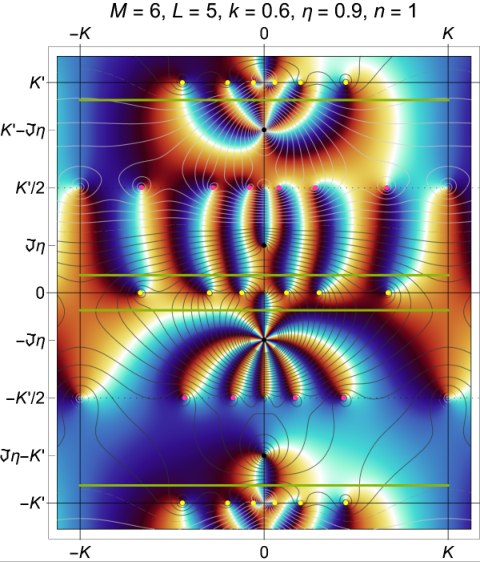
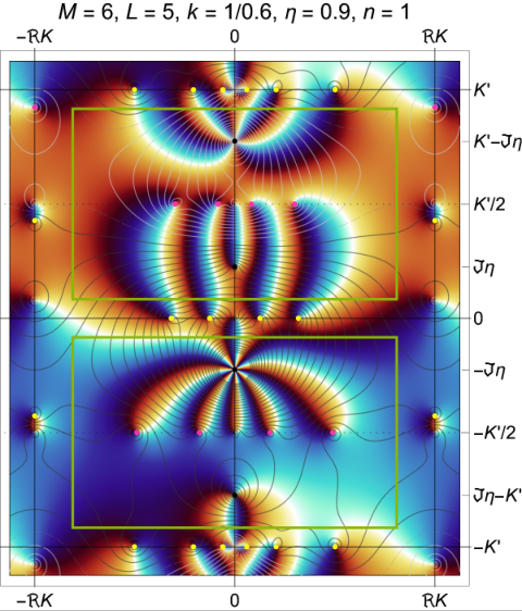
Figure 3: Complex structure of the integrand (3.27) for M=6M=6, L=5L=5, n=1n=1 and anisotropy η=0.9​ηiso\eta=0.9\,\eta_{\mathrm{iso}}, above (k=0.6k=0.6, left) and below (k−1=0.6k^{-1}=0.6, right) the critical point. Yellow: MM zeroes of the denominator, i. e., eigenvalues λμ\lambda_{\mu} of 𝐓\bm{\mathrm{T}}, and their para-conjugate. Pink: LL zeroes of the numerator and their para-conjugate. Black: multiple zeroes/poles from (2.18a), with pole order {−4,1,7,2}\{-4,1,7,2\} from top to bottom in this case. Green: possible integration paths. The contour lines are at constant modulus, with a dashed gray line at 1, and light (dark) gray lines at powers of 2 below (above) 1. The complex phase is color coded, being {white, red, black, blue} at {1,i,−1,−i}\{1,\mathrm{i},-1,-\mathrm{i}\}, such that white turns to red (blue) at zeroes (poles) under ccw. rotation. Note that KK becomes complex for k>1k>1.
Refer to caption
Refer to caption
Figure 4: Complex structure of the integrand (3.27) from figure 3 (left), mapped onto a torus. These pictures might (or might not) be helpful to better understand the setup. Left: the upper circle is the real axis, with the odd zeroes of the denominator (yellow), the outer circle has ℑ(u)=−K′/2\Im(u)=-K^{\prime}/2, with the even zeroes of the numerator (pink), and the black point in front is at −η-\eta. The remaining zeroes are inside and at the bottom. Right: The top circle is the imaginary axis ℜ⁡(u)=0\Re(u)=0, the front ring is the real axis. This representation corresponds to the original directions of the Ising model: the ↕\updownarrow direction goes along the 2​M2M denominator zeroes (yellow) from front to back, the ↔\leftrightarrow direction goes along the 2​L2L numerator zeroes (pink) from left to right, see also table 1.

The resulting integrand is shown in figures 3. At the four points {u0,∞,u∞,∞,u∞,0,u0,0}\{u_{0,\infty},u_{\infty,\infty},u_{\infty,0},u_{0,0}\} (2.18) (black dots), the pole orders1111 11 nn-fold poles (zeroes) have pole order nn (−n-n). {n+1−M,n+1+L−M,n+1+L,n+1}\{n+1-M,n+1+L-M,n+1+L,n+1\} are positive for certain n∈{1,…,M−1}n\in\{1,\ldots,M-1\}. As the additional zeroes at uˇμ\check{u}_{\mu} are removed, we can deform and simplify the integration contour CC to the four straight lines (green), which pairwise enclose the CP zeroes (yellow), or equivalently, the four points (2.18) (black dots). Due to the double periodic complex plane, the integration paths at ℜ⁡(u)=±K\Re(u)=\pm K add up to zero. Note that in the ordered phase below TcT_{\mathrm{c}} the smallest real zero u1u_{1} reaches ±K\pm K and becomes complex, such that the integration contour has to be modified as indicated. In figure 4 the complex torus is depicted.

Summarizing the last steps, we have found an extremely compact representation for the partition function of the anisotropic square lattice Ising model on the rectangle as the determinant of a Hankel matrix 𝐇=[hi+j+1]i,j=0M/2−1\bm{\mathrm{H}}=\left[\vphantom{A_{2}^{2}}h_{i+j+1}\right]_{i,j=0}^{M/2-1},

Z\displaystyle Z =Z1​det𝐇,\displaystyle=Z_{1}\det\bm{\mathrm{H}}, hn\displaystyle h_{n} =12​π​i​∮C1−eL​γ−θ1−ei⁡(M​φ−ω)​χn​∂γ∂u​𝑑u,\displaystyle=\frac{1}{2\pi\mathrm{i}}\oint_{C}\frac{1-\mathrm{e}^{L\gamma-\theta}}{1-\mathrm{e}^{\mathrm{i}(M\varphi-\omega)}}\,\chi^{n}\,\frac{\partial\gamma}{\partial u}\,\mathrm{d}u, (3.28)

with constant Z1Z_{1} from (3.23a). The hnh_{n} are Fourier coefficients (in the χ\chi base) of a so-called symbol function with Fisher-Hartwig type singularities (FisherHartwig68; HartwigFisher69) (see below), which is given by the ratio of two characteristic polynomials. These polynomials are associated with the two directions as well as the corresponding boundary conditions. As the considered system is invariant under an exchange of the two directions, the two CPs are directly related by the symmetry (1.5) of the underlying square lattice Ising model.

Note that the LL zeroes vℓv_{\ell} of the numerator 1−eL​γ−θ1-\mathrm{e}^{L\gamma-\theta} correspond to the LL eigenvalues of a hypothetical L×LL\times L transfer matrix 𝐓~\tilde{\bm{\mathrm{T}}} propagating in vertical direction, which would have been used in an alternative rotated setup. Only in the isotropic square system, where L=ML=M and 𝒦↔=𝒦↕\mathcal{K}^{\leftrightarrow}=\mathcal{K}^{\updownarrow}, these zeroes coincide with the swap-transformed zeroes, vℓ=𝒮⁡(uμ)=u~μv_{\ell}=\mathcal{S}(u_{\mu})=\tilde{u}_{\mu}. Unfortunately, we were not able to simplify the integral (3.28) in this symmetric case.

3.5 From Hankel to Toeplitz

The Hankel matrix (3.27) can be further transformed using the identities derived by Basor & Ehrhardt (BasorEhrhardt02). Using theorem 2.3, the symbols aa and bb, as well as the notation TM​(a)T_{M}(a), HM​(a)H_{M}(a) and HM​[b]H_{M}[b] from (BasorEhrhardt02), the determinant of 𝐇\bm{\mathrm{H}}, with elements (3.27), corresponds to the Hankel moment determinant detHM​[b]\det H_{M}[b] and can be transformed to the symmetric Toeplitz plus Hankel determinant det(TM​(a)+HM​(a))\det(T_{M}(a)+H_{M}(a)), with the symbol

a⁡(ζ)=e−ψ​b​(ζ+)=1−eL​γ−θ1−ei⁡(M​φ−ω)​∂γi​∂φ,a(\zeta)=\mathrm{e}^{-\psi}b(\zeta_{+})=\frac{1-\mathrm{e}^{L\gamma-\theta}}{1-\mathrm{e}^{\mathrm{i}(M\varphi-\omega)}}\,\frac{\partial\gamma}{\mathrm{i}\partial\varphi}, (3.29)

and with the Fourier components (BasorEhrhardt02, eq. (3))

an=a−n\displaystyle a_{n}=a_{-n} =12​π​∮Ca⁡(ei​φ)​e−i​n​φ​∂φ∂u​𝑑u\displaystyle=\frac{1}{2\pi}\oint_{C}a(\mathrm{e}^{\mathrm{i}\varphi})\,\mathrm{e}^{-\mathrm{i}n\varphi}\,\frac{\partial\varphi}{\partial u}\,\mathrm{d}u (3.30a)
=12​π​i​∮C1−eL​γ−θ1−ei⁡(M​φ−ω)​ζ−n​∂γ∂u​𝑑u.\displaystyle=\frac{1}{2\pi\mathrm{i}}\oint_{C}\frac{1-\mathrm{e}^{L\gamma-\theta}}{1-\mathrm{e}^{\mathrm{i}(M\varphi-\omega)}}\zeta^{-n}\,\frac{\partial\gamma}{\partial u}\,\mathrm{d}u. (3.30b)

Note that (3.29) transforms to its reciprocal, 𝒮⁡[a⁡(ζ)]=1/a⁡(ζ)\mathcal{S}[a(\zeta)]=1/a(\zeta), under exchange of the two directions. The advantage of this representation is the occurrence of the simpler Fourier base ζ−n\zeta^{-n}, which eliminates the poles in the integrand stemming from ζ→∞\zeta\to\infty at the points u∞,∞=ηu_{\infty,\infty}=\eta and u0,∞=i​K′−ηu_{0,\infty}=\mathrm{i}K^{\prime}-\eta, provided L<ML<M (as n≥0n\geq 0). We can therefore simplify the integration contour to a curve around the two remaining poles at u∞,0=−ηu_{\infty,0}=-\eta and u0,0=−i​K′+ηu_{0,0}=-\mathrm{i}K^{\prime}+\eta. However, for arbitrary LL and MM the pole order of the integrand (3.30b) at the four points (2.18) is {−n+2−M,−n+L−M,n+L,n}\{-n+2-M,-n+L-M,n+L,n\} and can be positive in all four cases, such that all four points must be enclosed by the contour.

Finally, from chapter 3 of (BasorEhrhardt02) we borrow a clever transformation from the symmetric Toeplitz plus Hankel representation to a skew-symmetric M×MM\times M Toeplitz matrix 𝐓^\hat{\bm{\mathrm{T}}}, with the result

𝐓^\displaystyle\hat{\bm{\mathrm{T}}} =[∑μ=1M2​i​t∗​eL​γμ−θμP𝝌′(χμ)sinφμ​cot⁡(12​φμ)​sin⁡[(i−j)​φμ]]i,j=0M−1\displaystyle=\left[\sum_{\mu=1}^{M}\frac{2\mathrm{i}t^{*}\,\mathrm{e}^{L\gamma_{\mu}-\theta_{\mu}}}{P_{\boldsymbol{\chi}}^{\prime}(\chi_{\mu})\sin\varphi_{\mu}}\cot(\tfrac{1}{2}\varphi_{\mu})\sin\!\big[(i-j)\varphi_{\mu}\big]\right]_{i,j=0}^{M-1} (3.31a)
=[1π​i​∮C1−eL​γ−θ1−ei⁡(M​φ−ω)​cot⁡(12​φ)​sin⁡[(i−j)​φ]​∂γ∂u​𝑑u]i,j=0M−1,\displaystyle=\left[\frac{1}{\pi\mathrm{i}}\oint_{C}\frac{1-\mathrm{e}^{L\gamma-\theta}}{1-\mathrm{e}^{\mathrm{i}(M\varphi-\omega)}}\cot(\tfrac{1}{2}\varphi)\sin\!\big[(i-j)\varphi\big]\,\frac{\partial\gamma}{\partial u}\,\mathrm{d}u\right]_{i,j=0}^{M-1}, (3.31b)
such that the Pfaffian of 𝐓^\hat{\bm{\mathrm{T}}} fulfills Pf⁡𝐓^=det𝐇\Pf\hat{\bm{\mathrm{T}}}=\det\bm{\mathrm{H}}, and therefore
Z=Z1​Pf⁡𝐓^.Z=Z_{1}\Pf\hat{\bm{\mathrm{T}}}. (3.31c)

As before, the integration contour CC can be freely deformed as long as it enclosed all zeroes uμu_{\mu} or, alternatively, the four points (2.18).

4 Discussion

In this work, we showed that the partition function of the anisotropic square lattice Ising model on the L×ML\times M rectangle with open boundary conditions in both directions is given by the determinant of a M/2×M/2\nicefrac{{M}}{{2}}\times\nicefrac{{M}}{{2}} Hankel matrix 𝐇\bm{\mathrm{H}}, which equivalently can be written as the Pfaffian of a skew-symmetric M×MM\times M Toeplitz matrix 𝐓^\hat{\bm{\mathrm{T}}}. The M−1M-1 independent matrix elements of 𝐇\bm{\mathrm{H}} or 𝐓^\hat{\bm{\mathrm{T}}} are Fourier coefficients of a symbol function (3.29), which is given by the ratio of two characteristic polynomials. These polynomials are associated to the two directions (↔,↕)(\leftrightarrow,\updownarrow) of the system, encode the respective boundary conditions, and are directly related through the symmetry of the square lattice Ising model under exchange of the two directions.

In the framework of the square lattice Ising model, Toeplitz matrices and determinants are well known in the context of bulk spatial correlation functions ⟨σ0,0​σℓ,m⟩\langle\sigma_{0,0}\sigma_{\ell,m}\rangle (FisherHartwig68; McCoyWu73; DeiftItsKrasovsky13), eventually leading to the spontaneous magnetization for ℓ2+m2​→∞\ell^{2}+m^{2}\text{$\to\infty$}. Surprisingly, they now also appear in the exact expressions for the partition function ZZ of finite systems.

The considered anisotropic Ising model with open BCs in both directions is invariant under exchange of the two directions ↔\leftrightarrow and ↕\updownarrow, such that both the system dimensions and the coupling constants are exchanged according to L↔𝒮ML\stackrel{{\scriptstyle\mathcal{S}}}{{\leftrightarrow}}M and 𝒦↔↔𝒮𝒦↕\mathcal{K}^{\leftrightarrow}\stackrel{{\scriptstyle\mathcal{S}}}{{\leftrightarrow}}\mathcal{K}^{\updownarrow}, see table 1. This swap transformation 𝒮\mathcal{S} (1.5) leads to the mapping of zz and tt to their respective duals, (z,t)↦𝒮(t∗,z∗)(z,t)\stackrel{{\scriptstyle\mathcal{S}}}{{\mapsto}}(t^{*},z^{*}), as well as to the exchange of the eigenvalues and angles according to λ↔𝒮ζ\lambda\stackrel{{\scriptstyle\mathcal{S}}}{{\leftrightarrow}}\zeta, γ↔𝒮i​φ\gamma\stackrel{{\scriptstyle\mathcal{S}}}{{\leftrightarrow}}\mathrm{i}\varphi and θ↔𝒮i​ω\theta\stackrel{{\scriptstyle\mathcal{S}}}{{\leftrightarrow}}\mathrm{i}\omega. In the complex uu-plane, it corresponds to a point reflection (u,η)↦𝒮(u~,η~)(u,\eta)\stackrel{{\scriptstyle\mathcal{S}}}{{\mapsto}}(\tilde{u},\tilde{\eta}) of the complex torus at the point ηiso=14​i​K′\eta_{\mathrm{iso}}={\textstyle\frac{1}{4}}\mathrm{i}K^{\prime} from (2.15). The elliptic modulus kk, however, is invariant under this transformation. This symmetry must not be confused with the related duality transformation 𝒟:(z,t∗)↦𝒟⁡[(z,t∗)]=(t,z∗)\mathcal{D}:(z,t^{*})\mapsto\mathcal{D}[(z,t^{*})]=(t,z^{*}) of the bulk system, which maps a low-temperature system with spins σℓ,m\sigma_{\ell,m} at k>1k>1 to a high-temperature system with the plaquette spins σ~ℓ,m\tilde{\sigma}_{\ell,m} at k↦k~=k−1<1k\mapsto\tilde{k}=k^{-1}<1, see figure 1. Note that in systems with boundaries, this transform is known to change the boundary conditions, e. g., from open to fixed.

Table 1: Overview over the quantities used in this work. The transformation 𝒮\mathcal{S} (1.5) maps between the two directions of the model. The right columns show the relation of our notation to the work of Baxter (Baxter16), where the transfer matrix propagated vertically.
direction ↔\leftrightarrow ↕\updownarrow ↕\updownarrow (Baxter16) ↔\leftrightarrow (Baxter16)
number of sites LL MM MM NN
reduced coupling 𝒦↔\mathcal{K}^{\leftrightarrow} 𝒦↕\mathcal{K}^{\updownarrow} HH H′H^{\prime}
weights (z,t)(z,t) (t∗,z∗)(t^{*},z^{*}) (t∗,u∗)(t^{*},u^{*}) (u,t)(u,t)
transfer matrix 𝓣\bm{\mathrm{\mathcal{T}}} 𝐐\bm{\mathrm{Q}} V^2​V^1\widehat{V}_{2}\widehat{V}_{1} −-
eigenvalues λ\lambda ζ\zeta λ\lambda zz
angles γ\gamma i​φ\mathrm{i}\varphi −- −-
boundary angles θ\theta i​ω\mathrm{i}\omega −- −-
characteristic polynomial 1−eL​γ−θ1-\mathrm{e}^{L\gamma-\theta} 1−ei⁡(M​φ−ω)1-\mathrm{e}^{\mathrm{i}(M\varphi-\omega)} −- (Baxter16, (3.21))
elliptic variables (u,η)(u,\eta) (u~,η~)(\tilde{u},\tilde{\eta}) (r,ν/2)(r,\nu/2) (r¯,ν¯/2)(\bar{r},\bar{\nu}/2)
elliptic modulus kk k−1k^{-1}
ℑ⁡(CP zeroes)\Im(\text{CP zeroes}) (0,K′)(0,K^{\prime}) ±K′/2\pm K^{\prime}/2 −- −-

During the present calculation, it was tried to find a representation of the partition function ZZ that is formally symmetric under the exchange of the two directions, mediated by the transformation 𝒮\mathcal{S}. While the symbol function a⁡(ζ)a(\zeta) from (3.29) already fulfills 𝒮⁡[a⁡(ζ)]=1/a⁡(ζ)\mathcal{S}[a(\zeta)]=1/a(\zeta), the transformation 𝒮\mathcal{S} exchanges the system dimensions L↔𝒮ML\stackrel{{\scriptstyle\mathcal{S}}}{{\leftrightarrow}}M and therefore changes the dimensions of the involved matrices, such that, e. g., a representation using (M+L)×(M+L)(M{+}L)\times(M{+}L) dimensional matrices might be necessary for a unified description.

The obtained results might possibly be rewritten using elliptic product identities, as done by Baxter (Baxter16) in the thermodynamic limit. The ultimate goal would be to use elliptic determinant evaluations as done successfully by Iorgov & Lisovyy (IorgovLisovyy11), which might lead to a closed product representation of the partition function.

We expect that our results can be extended to other boundary conditions by using the corresponding characteristic polynomials, these generalizations are left for future work.

From the Toeplitz determinant representation of the partition function, it is rather straightforward to derive the (anisotropic) scaling limit L,M→∞L,M\to\infty, T→TcT\to T_{\mathrm{c}} at fixed scaling variables x↕≡(T/Tc−1)​(M/ξ0↕)1/νx_{\updownarrow}\equiv(T/T_{\mathrm{c}}-1)(M/\xi_{0}^{\updownarrow})^{1/\nu} and ρ≡(L/ξ0↔)/(M/ξ0↕)\rho\equiv(L/\xi_{0}^{\leftrightarrow})/(M/\xi_{0}^{\updownarrow}) using Szegő’s theorem (Szego15; Szego20; DeiftItsKrasovsky13). This task will be addressed in a forthcoming work.

Acknowledgements.
The author is grateful to Hendrik Oppenberg, Felix M. Schmidt and Wolfhard Janke for helpful discussions and inspirations. Discussions with Jan Büddefeld, Luca Cervellera and Nils Gluth are acknowledged. This work was partially supported by the Deutsche Forschungsgemeinschaft through Grant HU 2303/1-1.

Appendix A Useful elliptic identities

In this appendix we will list identities arising from the elliptic parametrization. We also simplify expressions given in chapter VI of (Hucht16a). Following McCoy & Wu (McCoyWu14) (who used α1±1,α2±1\alpha_{1}^{\pm 1},\alpha_{2}^{\pm 1}) and Iorgov & Lisovyy (IorgovLisovyy11) (who used α±1,β±1\alpha^{\pm 1},\beta^{\pm 1}), we introduce abbreviations for products and ratios of zz and tt, however we again utilize Glashier’s notation (2.6) and define the constants

λn≡t​z,λs≡1t​z,λc≡tz,λd≡zt,{\lambda_{\mathrm{n}}}\equiv tz,\qquad{\lambda_{\mathrm{s}}}\equiv\frac{1}{tz},\qquad{\lambda_{\mathrm{c}}}\equiv\frac{t}{z},\qquad{\lambda_{\mathrm{d}}}\equiv\frac{z}{t}, (A.1)

with λn​λs=λc​λd=1{\lambda_{\mathrm{n}}}{\lambda_{\mathrm{s}}}={\lambda_{\mathrm{c}}}{\lambda_{\mathrm{d}}}=1. This leads to the identities

sn2⁡η\displaystyle\Jsn^{2}\eta =−λn​k−1,\displaystyle=-{\lambda_{\mathrm{n}}}k^{-1}, cn2⁡η\displaystyle\Jcn^{2}\eta =λnλn,−t​t−=1+λn​k−1,\displaystyle=\frac{{\lambda_{\mathrm{n}}}{\lambda_{\mathrm{n}}}_{,-}}{tt_{-}}=1+{\lambda_{\mathrm{n}}}k^{-1}, dn2⁡η\displaystyle\Jdn^{2}\eta =λnλn,−z​z−=1+λn​k.\displaystyle=\frac{{\lambda_{\mathrm{n}}}{\lambda_{\mathrm{n}}}_{,-}}{zz_{-}}=1+{\lambda_{\mathrm{n}}}k. (A.2)

Furthermore, We list relations to the primary reduced couplings 𝒦δ\mathcal{K}^{\delta} from (1.1),

t\displaystyle t =exp⁡(−2​𝒦↕),\displaystyle=\exp(-2\mathcal{K}^{\updownarrow}), t+\displaystyle t_{+} =cosh⁡(2​𝒦↕),\displaystyle=\cosh(2\mathcal{K}^{\updownarrow}), t−\displaystyle t_{-} =−sinh⁡(2​𝒦↕),\displaystyle=-\sinh(2\mathcal{K}^{\updownarrow}), (A.3a)
z\displaystyle z =tanh⁡𝒦↔,\displaystyle=\tanh\mathcal{K}^{\leftrightarrow}, z+\displaystyle z_{+} =coth⁡(2​𝒦↔),\displaystyle=\coth(2\mathcal{K}^{\leftrightarrow}), z−\displaystyle z_{-} =−csch⁡(2​𝒦↔),\displaystyle=-\csch(2\mathcal{K}^{\leftrightarrow}), (A.3b)
whereas for the dual couplings z∗,t∗z^{*},t^{*} the directions ↔\leftrightarrow and ↕\updownarrow are to be exchanged,
z∗\displaystyle z^{*} =exp⁡(−2​𝒦↔),\displaystyle=\exp(-2\mathcal{K}^{\leftrightarrow}), z∗+\displaystyle{z^{*}}_{\!+} =cosh⁡(2​𝒦↔),\displaystyle=\cosh(2\mathcal{K}^{\leftrightarrow}), z∗−\displaystyle{z^{*}}_{\!-} =−sinh⁡(2​𝒦↔),\displaystyle=-\sinh(2\mathcal{K}^{\leftrightarrow}), (A.3c)
t∗\displaystyle t^{*} =tanh⁡𝒦↕,\displaystyle=\tanh\mathcal{K}^{\updownarrow}, t∗+\displaystyle{t^{*}}_{\!+} =coth⁡(2​𝒦↕),\displaystyle=\coth(2\mathcal{K}^{\updownarrow}), t∗−\displaystyle{t^{*}}_{\!-} =−csch⁡(2​𝒦↕).\displaystyle=-\csch(2\mathcal{K}^{\updownarrow}). (A.3d)

Defining the dual primary reduced couplings 𝒦~δ\tilde{\mathcal{K}}^{\delta} via

exp⁡(−2​𝒦~δ)=tanh⁡𝒦δ,\exp(-2\tilde{\mathcal{K}}^{\delta})=\tanh\mathcal{K}^{\delta}, (A.4)

we conclude from (2.12) that the following simple relations hold between 𝒦~δ\tilde{\mathcal{K}}^{\delta} and η\eta,

2​i​𝒦~↕\displaystyle 2\mathrm{i}\tilde{\mathcal{K}}^{\updownarrow} =am⁡(2​η),\displaystyle=\Jam(2\eta), 2​i​𝒦~↔\displaystyle 2\mathrm{i}\tilde{\mathcal{K}}^{\leftrightarrow} =am⁡(2​η~),\displaystyle=\Jam(2\tilde{\eta}), (A.5)

such that the Jacobi amplitude (2.1) represents a direct connection between the physical reduced couplings 𝒦δ\mathcal{K}^{\delta} and the parameter η\eta, and (2.14) can be written using the elliptic Integral of the first kind, cf. (2.2),

2​η=F⁡(2​i​𝒦~↕,k)=i​K′−F⁡(2​i​𝒦~↔,k).2\eta=F(2\mathrm{i}\tilde{\mathcal{K}}^{\updownarrow},k)=\mathrm{i}K^{\prime}-F(2\mathrm{i}\tilde{\mathcal{K}}^{\leftrightarrow},k). (A.6)

We now turn to the eigenvalues λ\lambda and ζ\zeta. Defining the abbreviation

Q⁡(u,η)≡λn−λ=(k​sn2​η)2−1k​sn2​u−k​sn2​η,Q(u,\eta)\equiv\sqrt{{\lambda_{\mathrm{n}}}-\lambda}=\sqrt{\frac{(k\Jsn^{2}\eta)^{2}-1}{k\Jsn^{2}u-k\Jsn^{2}\eta}}, (A.7)

we can express the four roots from chapter VI of (Hucht16a) as meromorphic functions of uu, eliminating the ambiguous signs of the square roots,

λn−λ\displaystyle\sqrt{{\lambda_{\mathrm{n}}}-\lambda} =Q⁡(u,η)​nn⁡unn⁡η,\displaystyle=Q(u,\eta)\frac{\Jnn u}{\Jnn\eta}, λs−λ\displaystyle\sqrt{{\lambda_{\mathrm{s}}}-\lambda} =Q⁡(u,η)​sn⁡usn⁡η,\displaystyle=Q(u,\eta)\frac{\Jsn u}{\Jsn\eta}, (A.8a)
λc−λ\displaystyle\sqrt{{\lambda_{\mathrm{c}}}-\lambda} =Q⁡(u,η)​cn⁡ucn⁡η,\displaystyle=Q(u,\eta)\frac{\Jcn u}{\Jcn\eta}, λd−λ\displaystyle\sqrt{{\lambda_{\mathrm{d}}}-\lambda} =Q⁡(u,η)​dn⁡udn⁡η.\displaystyle=Q(u,\eta)\frac{\Jdn u}{\Jdn\eta}. (A.8b)

Note that we have used the trivial elliptic function nn⁡u≡1\Jnn u\equiv 1 in order to illustrate the systematics. Using (2.13) we can derive analog expressions for ζ\zeta,

ζn−ζ\displaystyle\sqrt{\zeta_{\mathrm{n}}-\zeta} =Q⁡(u~,η~)​nn⁡u~nn⁡η~,\displaystyle=Q(\tilde{u},\tilde{\eta})\frac{\Jnn\tilde{u}}{\Jnn\tilde{\eta}}, ζs−ζ\displaystyle\sqrt{\zeta_{\mathrm{s}}-\zeta} =Q⁡(u~,η~)​sn⁡u~sn⁡η~,\displaystyle=Q(\tilde{u},\tilde{\eta})\frac{\Jsn\tilde{u}}{\Jsn\tilde{\eta}}, (A.9a)
ζc−ζ\displaystyle\sqrt{\zeta_{\mathrm{c}}-\zeta} =Q⁡(u~,η~)​cn⁡u~cn⁡η~,\displaystyle=Q(\tilde{u},\tilde{\eta})\frac{\Jcn\tilde{u}}{\Jcn\tilde{\eta}}, ζd−ζ\displaystyle\sqrt{\zeta_{\mathrm{d}}-\zeta} =Q⁡(u~,η~)​dn⁡u~dn⁡η~,\displaystyle=Q(\tilde{u},\tilde{\eta})\frac{\Jdn\tilde{u}}{\Jdn\tilde{\eta}}, (A.9b)

where we defined

ζn≡z∗​t∗,ζs≡1z∗​t∗,ζc≡z∗t∗,ζd≡t∗z∗,\zeta_{\mathrm{n}}\equiv z^{*}t^{*},\qquad\zeta_{\mathrm{s}}\equiv\frac{1}{z^{*}t^{*}},\qquad\zeta_{\mathrm{c}}\equiv\frac{z^{*}}{t^{*}},\qquad\zeta_{\mathrm{d}}\equiv\frac{t^{*}}{z^{*}}, (A.10)

in analogy to (A.1). From (A.8a) and (A.9a) we further derive

λ\displaystyle\lambda =1−k2​sn2​u​sn2​ηk⁡(sn2⁡u−sn2⁡η),\displaystyle=\frac{1-k^{2}\Jsn^{2}u\Jsn^{2}\eta}{k(\Jsn^{2}u-\Jsn^{2}\eta)}, ζ\displaystyle\zeta =1−k2​sn2​u~​sn2​η~k⁡(sn2⁡u~−sn2⁡η~),\displaystyle=\frac{1-k^{2}\Jsn^{2}\tilde{u}\Jsn^{2}\tilde{\eta}}{k(\Jsn^{2}\tilde{u}-\Jsn^{2}\tilde{\eta})}, (A.11a)
which can be expressed using (1.2),
λ∗\displaystyle\lambda^{*} =−(k​sn2​u)∗(k​sn2​η)∗,\displaystyle=-\frac{(k\Jsn^{2}u)^{*}}{(k\Jsn^{2}\eta)^{*}}, ζ∗\displaystyle\zeta^{*} =−(k​sn2​u~)∗(k​sn2​η~)∗.\displaystyle=-\frac{(k\Jsn^{2}\tilde{u})^{*}}{(k\Jsn^{2}\tilde{\eta})^{*}}. (A.11b)

Inserting the elliptic expressions (A.8) into (I.46) we find

sin⁡φ2\displaystyle\sin\frac{\varphi}{2} =−λc−λ​λd−λ2​λ​t−​z−\displaystyle=-\frac{\sqrt{{\lambda_{\mathrm{c}}}-\lambda}\sqrt{{\lambda_{\mathrm{d}}}-\lambda}}{2\sqrt{\lambda t_{-}z_{-}}} =−Q2​(u,η)2​λ​t−​z−​cn⁡ucn⁡η​dn⁡udn⁡η,\displaystyle=-\frac{Q^{2}(u,\eta)}{2\sqrt{\lambda t_{-}z_{-}}}\frac{\Jcn u}{\Jcn\eta}\frac{\Jdn u}{\Jdn\eta}, (A.12a)
cos⁡φ2\displaystyle\cos\frac{\varphi}{2} =λn−λ​λs−λ2​i​λ​t−​z−\displaystyle=\frac{\sqrt{{\lambda_{\mathrm{n}}}-\lambda}\sqrt{{\lambda_{\mathrm{s}}}-\lambda}}{2\mathrm{i}\sqrt{\lambda t_{-}z_{-}}} =Q2​(u,η)2​i​λ​t−​z−​nn⁡unn⁡η​sn⁡usn⁡η,\displaystyle=\frac{Q^{2}(u,\eta)}{2\mathrm{i}\sqrt{\lambda t_{-}z_{-}}}\frac{\Jnn u}{\Jnn\eta}\frac{\Jsn u}{\Jsn\eta}, (A.12b)
tan⁡φ2\displaystyle\tan\frac{\varphi}{2} =1i​λc−λ​λd−λλn−λ​λs−λ\displaystyle=\frac{1}{\mathrm{i}}\frac{\sqrt{{\lambda_{\mathrm{c}}}-\lambda}\sqrt{{\lambda_{\mathrm{d}}}-\lambda}}{\sqrt{{\lambda_{\mathrm{n}}}-\lambda}\sqrt{{\lambda_{\mathrm{s}}}-\lambda}} =1i​nn⁡ηnn⁡u​sn⁡ηsn⁡u​cn⁡ucn⁡η​dn⁡udn⁡η,\displaystyle=\frac{1}{\mathrm{i}}\frac{\Jnn\eta}{\Jnn u}\frac{\Jsn\eta}{\Jsn u}\frac{\Jcn u}{\Jcn\eta}\frac{\Jdn u}{\Jdn\eta}, (A.12c)

while (I.47) at the eigenvalues λμ\lambda_{\mu} become

±sin⁡M​φμ2\displaystyle\pm\sin\frac{M\varphi_{\mu}}{2} =t​λs−λμ​λd−λμ2​λμ​t−​λμ,−\displaystyle=\sqrt{t}\frac{\sqrt{{\lambda_{\mathrm{s}}}-\lambda_{\mu}}\sqrt{{\lambda_{\mathrm{d}}}-\lambda_{\mu}}}{2\sqrt{\lambda_{\mu}t_{-}\lambda_{\mu,-}}} =t2​Q2​(uμ,η)λμ​t−​λμ,−​sn⁡uμsn⁡η​dn⁡uμdn⁡η,\displaystyle=\frac{\sqrt{t}}{2}\frac{Q^{2}(u_{\mu},\eta)}{\sqrt{\lambda_{\mu}t_{-}\lambda_{\mu,-}}}\frac{\Jsn u_{\mu}}{\Jsn\eta}\frac{\Jdn u_{\mu}}{\Jdn\eta}, (A.13a)
±cos⁡M​φμ2\displaystyle\pm\cos\frac{M\varphi_{\mu}}{2} =1t​λn−λμ​λc−λμ2​i​λμ​t−​λμ,−\displaystyle=\frac{1}{\sqrt{t}}\frac{\sqrt{{\lambda_{\mathrm{n}}}-\lambda_{\mu}}\sqrt{{\lambda_{\mathrm{c}}}-\lambda_{\mu}}}{2\mathrm{i}\sqrt{\lambda_{\mu}t_{-}\lambda_{\mu,-}}} =12​i​t​Q2​(uμ,η)λμ​t−​λμ,−​nn⁡uμnn⁡η​cn⁡uμcn⁡η,\displaystyle=\frac{1}{2\mathrm{i}\sqrt{t}}\frac{Q^{2}(u_{\mu},\eta)}{\sqrt{\lambda_{\mu}t_{-}\lambda_{\mu,-}}}\frac{\Jnn u_{\mu}}{\Jnn\eta}\frac{\Jcn u_{\mu}}{\Jcn\eta}, (A.13b)
tan⁡M​φμ2\displaystyle\tan\frac{M\varphi_{\mu}}{2} =i​t​λs−λμ​λd−λμλn−λμ​λc−λμ\displaystyle=\mathrm{i}t\frac{\sqrt{{\lambda_{\mathrm{s}}}-\lambda_{\mu}}\sqrt{{\lambda_{\mathrm{d}}}-\lambda_{\mu}}}{\sqrt{{\lambda_{\mathrm{n}}}-\lambda_{\mu}}\sqrt{{\lambda_{\mathrm{c}}}-\lambda_{\mu}}} =sn⁡uμ​dn⁡uμnn⁡uμ​cn⁡uμ.\displaystyle=\frac{\Jsn u_{\mu}\Jdn u_{\mu}}{\Jnn u_{\mu}\Jcn u_{\mu}}. (A.13c)

We additionally list the identities

t−​z−​i​sin⁡φ\displaystyle t_{-}z_{-}\mathrm{i}\sin\varphi =−12​λ​λn−λ​λs−λ​λc−λ​λd−λ\displaystyle=-\frac{1}{2\lambda}\sqrt{{\lambda_{\mathrm{n}}}-\lambda}\sqrt{{\lambda_{\mathrm{s}}}-\lambda}\sqrt{{\lambda_{\mathrm{c}}}-\lambda}\sqrt{{\lambda_{\mathrm{d}}}-\lambda} (A.14a)
=λs,+−λ+​λd,+−λ+\displaystyle=\sqrt{{\lambda_{\mathrm{s}}}_{,+}-\lambda_{+}}\sqrt{{\lambda_{\mathrm{d}}}_{,+}-\lambda_{+}} (A.14b)
=−Q4​(u,η)2​λ​nn⁡unn⁡η​sn⁡usn⁡η​cn⁡ucn⁡η​dn⁡udn⁡η.\displaystyle=-\frac{Q^{4}(u,\eta)}{2\lambda}\frac{\Jnn u}{\Jnn\eta}\frac{\Jsn u}{\Jsn\eta}\frac{\Jcn u}{\Jcn\eta}\frac{\Jdn u}{\Jdn\eta}. (A.14c)
as well as
2​t−​z−​i​sin⁡φ2\displaystyle\sqrt{2t_{-}z_{-}}\,\mathrm{i}\sin\frac{\varphi}{2} =λd,+−λ+,\displaystyle=\sqrt{{\lambda_{\mathrm{d}}}_{,+}-\lambda_{+}}, 2​t−​z−​cos⁡φ2\displaystyle\sqrt{2t_{-}z_{-}}\cos\frac{\varphi}{2} =λs,+−λ+.\displaystyle=\sqrt{{\lambda_{\mathrm{s}}}_{,+}-\lambda_{+}}. (A.14d)

Using the addition theorem (Lawden89, (2.4.22))

k​sn⁡u​sn⁡v=k​cn⁡(u−v)−cn⁡(u+v)dn⁡(u−v)+dn⁡(u+v)=1k​dn⁡(u−v)−dn⁡(u+v)cn⁡(u−v)+cn⁡(u+v)k\Jsn u\,\Jsn v=k\frac{\Jcn(u-v)-\Jcn(u+v)}{\Jdn(u-v)+\Jdn(u+v)}=\frac{1}{k}\frac{\Jdn(u-v)-\Jdn(u+v)}{\Jcn(u-v)+\Jcn(u+v)} (A.15)

we derive the important identities

λ=eγ\displaystyle\lambda=\mathrm{e}^{\gamma} =−k​cn⁡(2​u)+cn⁡(2​η)dn⁡(2​u)−dn⁡(2​η)=−1k​dn⁡(2​u)+dn⁡(2​η)cn⁡(2​u)−cn⁡(2​η),\displaystyle=-k\frac{\Jcn(2u)+\Jcn(2\eta)}{\Jdn(2u)-\Jdn(2\eta)}=-\frac{1}{k}\frac{\Jdn(2u)+\Jdn(2\eta)}{\Jcn(2u)-\Jcn(2\eta)}, (A.16a)
λ+=cosh⁡γ\displaystyle\lambda_{+}=\cosh\gamma =−k​cn⁡(2​u)​dn⁡(2​u)+cn⁡(2​η)​dn⁡(2​η)dn2⁡(2​u)−dn2⁡(2​η),\displaystyle=-k\frac{\Jcn(2u)\Jdn(2u)+\Jcn(2\eta)\Jdn(2\eta)}{\Jdn^{2}(2u)-\Jdn^{2}(2\eta)}, (A.16b)
λ−=sinh⁡γ\displaystyle\lambda_{-}=\sinh\gamma =−k​cn⁡(2​u)​dn⁡(2​η)+cn⁡(2​η)​dn⁡(2​u)dn2⁡(2​u)−dn2⁡(2​η),\displaystyle=-k\frac{\Jcn(2u)\Jdn(2\eta)+\Jcn(2\eta)\Jdn(2u)}{\Jdn^{2}(2u)-\Jdn^{2}(2\eta)}, (A.16c)

and, by the swap transformation (2.13),

ζ=ei​φ\displaystyle\zeta=\mathrm{e}^{\mathrm{i}\varphi} =−ds⁡(2​u)+ds⁡(2​η)cs⁡(2​u)−cs⁡(2​η)=−cs⁡(2​u)+cs⁡(2​η)ds⁡(2​u)−ds⁡(2​η),\displaystyle=-\frac{\Jds(2u)+\Jds(2\eta)}{\Jcs(2u)-\Jcs(2\eta)}=-\frac{\Jcs(2u)+\Jcs(2\eta)}{\Jds(2u)-\Jds(2\eta)}, (A.17a)
ζ+=cos⁡φ\displaystyle\zeta_{+}=\cos\varphi =−ds⁡(2​u)​cs⁡(2​u)+ds⁡(2​η)​cs⁡(2​η)cs2⁡(2​u)−cs2⁡(2​η),\displaystyle=-\frac{\Jds(2u)\Jcs(2u)+\Jds(2\eta)\Jcs(2\eta)}{\Jcs^{2}(2u)-\Jcs^{2}(2\eta)}, (A.17b)
ζ−=i​sin⁡φ\displaystyle\zeta_{-}=\mathrm{i}\sin\varphi =−ds⁡(2​u)​cs⁡(2​η)+ds⁡(2​η)​cs⁡(2​u)cs2⁡(2​u)−cs2⁡(2​η),\displaystyle=-\frac{\Jds(2u)\Jcs(2\eta)+\Jds(2\eta)\Jcs(2u)}{\Jcs^{2}(2u)-\Jcs^{2}(2\eta)}, (A.17c)

which express the eigenvalues λ\lambda and ζ\zeta as functions of 2​u2u.

We now turn to derivatives. From (2.16) and

∂∂u​log⁡sn⁡(u±η)=cn⁡(u±η)​dn⁡(u±η)sn⁡(u±η)=k​λ−​[sn⁡(2​u)∓sn⁡(2​η)]\frac{\partial}{\partial u}\log\Jsn(u\pm\eta)=\frac{\Jcn(u\pm\eta)\Jdn(u\pm\eta)}{\Jsn(u\pm\eta)}=k\lambda_{-}[\Jsn(2u)\mp\Jsn(2\eta)] (A.18)

we see that the derivatives of φ\varphi and γ\gamma w.r.t. uu become

12​∂φ∂u\displaystyle\frac{1}{2}\frac{\partial\varphi}{\partial u} =i​k​sn⁡(2​η)​λ−\displaystyle=\,\,\mathrm{i}k\Jsn(2\eta)\,\lambda_{-} =1z−​sinh⁡γ\displaystyle=\frac{1}{z_{-}}\sinh\gamma =−sin⁡φsin⁡ω,\displaystyle=-\frac{\sin\varphi}{\sin\omega}, (A.19a)
12​∂γ∂u\displaystyle\frac{1}{2}\frac{\partial\gamma}{\partial u} =−k​sn⁡(2​u)​λ−\displaystyle=-k\Jsn(2u)\,\lambda_{-} =t−​sin⁡φ\displaystyle=t_{-}\sin\varphi =i​sinh⁡γsinh⁡θ,\displaystyle=\mathrm{i}\frac{\sinh\gamma}{\sinh\theta}, (A.19b)

from which other identities, such as

∂γ∂φ=−t−​sin⁡ω=t−​z−​sin⁡φsinh⁡γ,∂χ∂u=χ2−4sin⁡ω,\frac{\partial\gamma}{\partial\varphi}=-t_{-}\sin\omega=t_{-}z_{-}\frac{\sin\varphi}{\sinh\gamma},\qquad\frac{\partial\chi}{\partial u}=\frac{\chi^{2}-4}{\sin\omega}, (A.20)

are easily calculated.

In the ordered phase where k>1k>1, the angle φ1\varphi_{1} becomes complex (Hucht16a, chap. 6), leading to a complex value of u1u_{1}. The correct mapping from the eigenvalues λμ\lambda_{\mu} to the elliptic variable uμu_{\mu}, respecting this behavior and being valid at arbitrary temperatures, can be expressed using the inverse Jacobi dn, see (A.8),

uμ=dn(−1)⁡[dn⁡η​λd−λμλn−λμ].u_{\mu}=\Jdn^{(-1)}\negmedspace\left[\Jdn\eta\,\frac{\sqrt{{\lambda_{\mathrm{d}}}-\lambda_{\mu}}}{\sqrt{{\lambda_{\mathrm{n}}}-\lambda_{\mu}}}\right]. (A.21)

While it is tempting to utilize the simpler relation (2.19)

uμ=12​F​(M​φμ,k),u_{\mu}=\frac{1}{2}F(M\varphi_{\mu},k), (A.22)

it won’t give correct results for even μ\mu and below TcT_{\mathrm{c}}, because the elliptic integral FF does not have the correct branch cut positions for these cases.

Appendix B A block Hankel matrix identity

Let 𝓥𝒈,𝒙\bm{\mathrm{\mathcal{V}}}_{\boldsymbol{g},\boldsymbol{x}} be the generalized 1×B1\times B block Vandermonde matrix with M×NM\times N blocks

𝓥𝒈,𝒙≡[gμb​xμn]b=0;μ=1,n=0B−1​M​N−1=[𝐆b​𝐕𝒙]b=0B−1,\bm{\mathrm{\mathcal{V}}}_{\boldsymbol{g},\boldsymbol{x}}\equiv\left[\vphantom{A_{2}^{2}}g_{\mu}^{b}\,x_{\mu}^{n}\right]_{b=0;\,\,\mu=1,\,n=0}^{B-1\,M\hskip 6.02777ptN-1}=\left[\vphantom{A_{2}^{2}}\bm{\mathrm{G}}^{b}\,\bm{\mathrm{V}}_{\!\boldsymbol{x}}\right]_{b=0}^{B-1}, (B.1)

with

𝐕𝒙≡[xμn]μ=1,n=0M​N−1,𝐆≡[δμ​ν​gμ]μ,ν=1M.\bm{\mathrm{V}}_{\!\boldsymbol{x}}\equiv\left[\vphantom{A_{2}^{2}}x_{\mu}^{n}\right]_{\mu=1,\,n=0}^{M\hskip 6.02777ptN-1},\qquad\bm{\mathrm{G}}\equiv\left[\vphantom{A_{2}^{2}}\delta_{\mu\nu}\,g_{\mu}\right]_{\mu,\nu=1}^{M}. (B.2)

As an example, for M=4M=4, B=3B=3 and N=3N=3 we have

𝓥𝒈,𝒙=[1x1x12g1g1​x1g1​x12g12g12​x1g12​x121x2x22g2g2​x2g2​x22g22g22​x2g22​x221x3x32g3g3​x3g3​x32g32g32​x3g32​x321x4x42g4g4​x4g4​x42g42g42​x4g42​x42].\bm{\mathrm{\mathcal{V}}}_{\boldsymbol{g},\boldsymbol{x}}=\left[\begin{array}[]{ccc|ccc|ccc}1&x_{1}&x_{1}^{2}&g_{1}&g_{1}x_{1}&g_{1}x_{1}^{2}&g_{1}^{2}&g_{1}^{2}x_{1}&g_{1}^{2}x_{1}^{2}\\ 1&x_{2}&x_{2}^{2}&g_{2}&g_{2}x_{2}&g_{2}x_{2}^{2}&g_{2}^{2}&g_{2}^{2}x_{2}&g_{2}^{2}x_{2}^{2}\\ 1&x_{3}&x_{3}^{2}&g_{3}&g_{3}x_{3}&g_{3}x_{3}^{2}&g_{3}^{2}&g_{3}^{2}x_{3}&g_{3}^{2}x_{3}^{2}\\ 1&x_{4}&x_{4}^{2}&g_{4}&g_{4}x_{4}&g_{4}x_{4}^{2}&g_{4}^{2}&g_{4}^{2}x_{4}&g_{4}^{2}x_{4}^{2}\end{array}\right]. (B.3)

Furthermore, let 𝐃\bm{\mathrm{D}} be an arbitrary M×MM\times M diagonal matrix. Then, the B×BB\times B block Hankel matrix with N×NN\times N blocks

𝓗𝒈,𝒙≡[∑μ=1Mdμ​gμa+b​xμm+n]a,b=0;m,n=0B−1​N−1=[𝐕𝒙⊤​𝐃​𝐆a+b​𝐕𝒙]a,b=0B−1\bm{\mathrm{\mathcal{H}}}_{\boldsymbol{g},\boldsymbol{x}}\equiv\left[\sum_{\mu=1}^{M}d_{\mu}g_{\mu}^{a+b}\,x_{\mu}^{m+n}\right]_{a,b=0;\,m,n=0}^{B-1\;\;\;N-1}=\left[\bm{\mathrm{V}}^{\top}_{\!\boldsymbol{x}}\,\bm{\mathrm{D}}\,\bm{\mathrm{G}}^{a+b}\,\bm{\mathrm{V}}_{\!\boldsymbol{x}}\right]_{a,b=0}^{B-1} (B.4)

trivially fulfills the identity

𝓗𝒈,𝒙=𝓥𝒈,𝒙⊤​𝐃​𝓥𝒈,𝒙.\bm{\mathrm{\mathcal{H}}}_{\boldsymbol{g},\boldsymbol{x}}=\bm{\mathrm{\mathcal{V}}}^{\top}_{\!\boldsymbol{g},\boldsymbol{x}}\bm{\mathrm{D}}\bm{\mathrm{\mathcal{V}}}_{\!\boldsymbol{g},\boldsymbol{x}}. (B.5)

Note that the upper left block (𝓗𝒈,𝒙)0,0=𝐕𝒙⊤​𝐃​𝐕𝒙(\bm{\mathrm{\mathcal{H}}}_{\boldsymbol{g},\boldsymbol{x}})_{0,0}=\bm{\mathrm{V}}^{\top}_{\!\boldsymbol{x}}\,\bm{\mathrm{D}}\,\bm{\mathrm{V}}_{\!\boldsymbol{x}} is free of gμg_{\mu} and is therefore a usual Vandermonde product in xμx_{\mu}. Consequently, if the matrix 𝐃\bm{\mathrm{D}} is set to the diagonal matrix 𝐃𝒙\bm{\mathrm{D}}_{\boldsymbol{x}} with the reciprocal first derivatives of the characteristic polynomial P𝒙​(x)P_{\boldsymbol{x}}(x) from (3.17),

𝐃𝒙≡[δμ​νP𝒙′​(xμ)]μ,ν=1M,\bm{\mathrm{D}}_{\boldsymbol{x}}\equiv\left[\frac{\delta_{\mu\nu}}{P_{\boldsymbol{x}}^{\prime}(x_{\mu})}\right]_{\mu,\nu=1}^{M}, (B.6)

and if additionally M≥2​NM\geq 2N, then (𝐇𝒈,𝒙)0,0(\bm{\mathrm{H}}_{\boldsymbol{g},\boldsymbol{x}})_{0,0} vanishes identically. For B=2B=2 and N=M/2N=M/2, this leads to equation (3.20).

Appendix C More characteristic polynomials

In (Hucht16b) we used the finite-size scaling limit of P𝝀+P_{\boldsymbol{\lambda_{+}}} to locate the zeroes in the complex plane and to perform the corresponding Cauchy integrals. We had to distinguish between even and odd zeroes and defined an alternating counting polynomial from P𝝀+P_{\boldsymbol{\lambda_{+}}}. Now we will demonstrate that it is much easier to analyze the complex structure of the system by using the CP of the transfer matrix 𝐓\bm{\mathrm{T}} instead of 𝐓+\bm{\mathrm{T}}_{+}. While it is possible but cumbersome to derive the CP of 𝐓\bm{\mathrm{T}}, with eigenvalues λμ\lambda_{\mu},

P𝝀​(λ)≡det(λ​𝟏−𝐓)=∏μ=1M(λ−λμ)P_{\boldsymbol{\lambda}}(\lambda)\equiv\det(\lambda\bm{\mathrm{1}}-\bm{\mathrm{T}})=\prod_{\mu=1}^{M}(\lambda-\lambda_{\mu}) (C.1)

from scratch analogously to (1.24a), cf. (Hucht16a), we instead proceed in a much simpler way and derive it directly from (3.2): Using (1.3), we first factorize the right hand side of (1.24a),

P𝝀+​(λ+)=∏μ=1M(λ+−λμ,+)=∏μ=1M(λ−λμ)​(λ−1−λμ)2​(0−λμ)=12M​t​P𝝀​(λ)​P𝝀​(λ−1),P_{\boldsymbol{\lambda_{+}}}(\lambda_{+})=\prod_{\mu=1}^{M}(\lambda_{+}-\lambda_{\mu,+})=\prod_{\mu=1}^{M}\frac{(\lambda-\lambda_{\mu})(\lambda^{-1}-\lambda_{\mu})}{2(0-\lambda_{\mu})}=\frac{1}{2^{M}t}P_{\boldsymbol{\lambda}}(\lambda)P_{\boldsymbol{\lambda}}(\lambda^{-1}), (C.2)

as λμ,+=λ+.μ\lambda_{\mu,+}=\lambda_{+.\mu} and, cf. (I.35),

P𝝀​(0)=det(−𝐓)=det𝐓=t.P_{\boldsymbol{\lambda}}(0)=\det(-\bm{\mathrm{T}})=\det\bm{\mathrm{T}}=t. (C.3)

Employing the trigonometric factorization identity

sin⁡(M​φ−ω)sin⁡(−ω)=sin⁡(12​[M​φ−ω])sin⁡(−12​ω)​cos⁡(12​[M​φ−ω])cos⁡(−12​ω)\frac{\sin\left(M\varphi-\omega\right)}{\sin(-\omega)}=\frac{\sin\left({\textstyle\frac{1}{2}}[M\varphi-\omega]\right)}{\sin\left(-{\textstyle\frac{1}{2}}\omega\right)}\frac{\cos\left({\textstyle\frac{1}{2}}[M\varphi-\omega]\right)}{\cos\left(-{\textstyle\frac{1}{2}}\omega\right)} (C.4)

as well as the identities

λ⁡(uˇ)​λ​(u)=1,φ⁡(uˇ)=−φ⁡(u),ω⁡(uˇ)+ω⁡(u)=π,cot⁡[12​ω​(uˇ)]=tan⁡[12​ω​(u)],\lambda(\check{u})\lambda(u)=1,\quad\varphi(\check{u})=-\varphi(u),\quad\omega(\check{u})+\omega(u)=\pi,\quad\cot[{\textstyle\frac{1}{2}}\omega(\check{u})]=\tan[{\textstyle\frac{1}{2}}\omega(u)], (C.5)

with inversion transform u↦uˇ≡u+i​K′u\mapsto\check{u}\equiv u+\mathrm{i}K^{\prime}, we see that P𝝀​(λ)P_{\boldsymbol{\lambda}}(\lambda) and P𝝀​(λ−1)P_{\boldsymbol{\lambda}}(\lambda^{-1}) are given by the remarkably simple formulas

P𝝀​(λ)\displaystyle P_{\boldsymbol{\lambda}}(\lambda) =(1−t∗)​(−t−​z−​λ)M2​[cos⁡(12​M​φ)−cot⁡(12​ω)​sin⁡(12​M​φ)]\displaystyle=(1-t^{*})\left(-t_{-}z_{-}\lambda\right)^{\frac{M}{2}}\left[\cos\left({\textstyle\frac{1}{2}}M\varphi\right)-\cot\left({\textstyle\frac{1}{2}}\omega\right)\sin\left({\textstyle\frac{1}{2}}M\varphi\right)\right] (C.6a)
=(1−t∗)​(−t−​z−​λ)M2​sin⁡(12​[M​φ−ω])sin⁡(−12​ω)\displaystyle=(1-t^{*})\left(-t_{-}z_{-}\lambda\right)^{\frac{M}{2}}\frac{\sin\left({\textstyle\frac{1}{2}}[M\varphi-\omega]\right)}{\sin\left(-{\textstyle\frac{1}{2}}\omega\right)} (C.6b)
=(1−t∗)​(−t−​z−​λζ)M2​1−ei⁡(M​φ−ω)1−e−i​ω,\displaystyle=(1-t^{*})\left(-\frac{t_{-}z_{-}\lambda}{\zeta}\right)^{\negmedspace\frac{M}{2}}\frac{1-\mathrm{e}^{\mathrm{i}(M\varphi-\omega)}}{1-\mathrm{e}^{-\mathrm{i}\omega}}, (C.6c)
P𝝀​(λ−1)\displaystyle P_{\boldsymbol{\lambda}}(\lambda^{-1}) =(1−t∗)​(−t−​z−​λ−1)M2​[cos⁡(12​M​φ)+tan⁡(12​ω)​sin⁡(12​M​φ)]\displaystyle=(1-t^{*})\left(-t_{-}z_{-}\lambda^{-1}\right)^{\frac{M}{2}}\left[\cos\left({\textstyle\frac{1}{2}}M\varphi\right)+\tan\left({\textstyle\frac{1}{2}}\omega\right)\sin\left({\textstyle\frac{1}{2}}M\varphi\right)\right] (C.6d)
=(1−t∗)​(−t−​z−​λ−1)M2​cos⁡(12​[M​φ−ω])cos⁡(−12​ω)\displaystyle=(1-t^{*})\left(-t_{-}z_{-}\lambda^{-1}\right)^{\frac{M}{2}}\frac{\cos\left({\textstyle\frac{1}{2}}[M\varphi-\omega]\right)}{\cos\left(-{\textstyle\frac{1}{2}}\omega\right)} (C.6e)
=(1−t∗)​(−t−​z−λ​ζ)M2​1+ei⁡(M​φ−ω)1+e−i​ω,\displaystyle=(1-t^{*})\left(-\frac{t_{-}z_{-}}{\lambda\zeta}\right)^{\negmedspace\frac{M}{2}}\frac{1+\mathrm{e}^{\mathrm{i}(M\varphi-\omega)}}{1+\mathrm{e}^{-\mathrm{i}\omega}}, (C.6f)

The additional factor (−λ)M/2(-\lambda)^{M/2} in P𝝀​(λ)P_{\boldsymbol{\lambda}}(\lambda) follows from (C.3) in the known limits λ→{0,∞}\lambda\to\{0,\infty\}, see (2.18). Utilizing a factorization similar to (C.2), the CP of 𝐓−\bm{\mathrm{T}}_{-} can also be derived,

P𝝀−​(λ−)=∏μ=1M(λ−−λμ,−)=∏μ=1M(λ−λμ)​(−λ−1−λμ)2​(0−λμ)=12M​t​P𝝀​(λ)​P𝝀​(−λ−1).P_{\boldsymbol{\lambda_{-}}}(\lambda_{-})=\prod_{\mu=1}^{M}(\lambda_{-}-\lambda_{\mu,-})=\prod_{\mu=1}^{M}\frac{(\lambda-\lambda_{\mu})(-\lambda^{-1}-\lambda_{\mu})}{2(0-\lambda_{\mu})}=\frac{1}{2^{M}t}P_{\boldsymbol{\lambda}}(\lambda)P_{\boldsymbol{\lambda}}(-\lambda^{-1}). (C.7)

Finally, from (3.25) and Liouville’s theorem (Baxter82, 15.3) we derived the CPs

P𝜻​(ζ)\displaystyle P_{\boldsymbol{\zeta}}(\zeta) =(1−t∗)​1−ei⁡(M​φ−ω)1−e−i​ω​∏μ=1Msn⁡(η+uμ)sn⁡(u+uμ),\displaystyle=(1-t^{*})\frac{1-\mathrm{e}^{\mathrm{i}(M\varphi-\omega)}}{1-\mathrm{e}^{-\mathrm{i}\omega}}\prod_{\mu=1}^{M}\frac{\Jsn(\eta+u_{\mu})}{\Jsn(u+u_{\mu})}, (C.8)
P𝜻​(ζ−1)\displaystyle P_{\boldsymbol{\zeta}}(\zeta^{-1}) =(1−t∗)​1+e−i⁡(M​φ−ω)1+ei​ω​∏μ=1Mk​sn⁡(η+uμ)​sn⁡(u+uμ).\displaystyle=(1-t^{*})\frac{1+\mathrm{e}^{-\mathrm{i}(M\varphi-\omega)}}{1+\mathrm{e}^{\mathrm{i}\omega}}\prod_{\mu=1}^{M}k\Jsn(\eta+u_{\mu})\Jsn(u+u_{\mu}). (C.9)

Appendix D Some product identities

Using the CPs (3.2), (C.6), (C.7), we have the following identities (remember that MM is even): the determinants are given by

det𝐓\displaystyle\det\bm{\mathrm{T}}_{\hphantom{-}} =∏μ=1Mλμ=P𝝀​(0)=t,\displaystyle=\prod_{\mu=1}^{M}\lambda_{\mu\hphantom{,-}}=P_{\boldsymbol{\lambda}}(0)_{\hphantom{-}}=t\,, (D.1a)
det𝐓−\displaystyle\det\bm{\mathrm{T}}_{-} =∏μ=1Mλμ,−=P𝝀−​(0)=(1−t∗2)​(i​z−1−t∗2)M,\displaystyle=\prod_{\mu=1}^{M}\lambda_{\mu,-}=P_{\boldsymbol{\lambda_{-}}}(0)=(1-{t^{*}}^{2})\left(\frac{\mathrm{i}z_{-}}{1-{t^{*}}^{2}}\right)^{\negmedspace M}\negmedspace, (D.1b)
det𝐓+\displaystyle\det\bm{\mathrm{T}}_{+} =∏μ=1Mλμ,+=P𝝀+​(0)=(1−t∗2)​(t−​z−2)M​sin⁡(M​φλ+→0−ωλ+→0)sin⁡(−ωλ+→0),\displaystyle=\prod_{\mu=1}^{M}\lambda_{\mu,+}=P_{\boldsymbol{\lambda_{+}}}(0)=(1-{t^{*}}^{2})\left(\frac{t_{-}z_{-}}{2}\right)^{\negmedspace M}\frac{\sin(M\varphi_{\lambda_{+}\to 0}-\omega_{\lambda_{+}\to 0})}{\sin(-\omega_{\lambda_{+}\to 0})}, (D.1c)

with (2.18) and

uλ+→0=sn(−1)⁡(i​λn)∗i​k,uλ−→0=K+12​i​K′.u_{\lambda_{+}\to 0}=\Jsn^{(-1)}\sqrt{\frac{(\mathrm{i}{\lambda_{\mathrm{n}}})^{*}}{\mathrm{i}k}},\qquad u_{\lambda_{-}\to 0}=K+\tfrac{1}{2}\mathrm{i}K^{\prime}. (D.2)

Furthermore, we have the following product identities for the Jacobi elliptic functions

∏μ=1M−t​z​sn⁡uμsn⁡η\displaystyle\prod_{\mu=1}^{M}\sqrt{-tz}\,\frac{\Jsn u_{\mu}}{\Jsn\eta} =1−Mλs,−z−−1,\displaystyle=\sqrt{1-M{\lambda_{\mathrm{s}}}_{,-}z_{-}^{-1}}\,, (D.3a)
∏μ=1Mi​z​cn⁡uμcn⁡η\displaystyle\prod_{\mu=1}^{M}\sqrt{\mathrm{i}z}\,\frac{\Jcn u_{\mu}}{\Jcn\eta} =1,\displaystyle=1\,, (D.3b)
∏μ=1Mi​t​dn⁡uμdn⁡η\displaystyle\prod_{\mu=1}^{M}\sqrt{\mathrm{i}t}\,\frac{\Jdn u_{\mu}}{\Jdn\eta} =1+Mλd,−z−−1.\displaystyle=\sqrt{1+M{\lambda_{\mathrm{d}}}_{,-}z_{-}^{-1}}\,. (D.3c)

For products over λμ\lambda_{\mu} we find the identities

∏μ=1M(λn−λμ)\displaystyle\prod_{\mu=1}^{M}({\lambda_{\mathrm{n}}}-\lambda_{\mu}) =P𝝀​(λn)=(1−t∗)​(t−​z−​λn)M2,\displaystyle=P_{\boldsymbol{\lambda}}({\lambda_{\mathrm{n}}})=(1-t^{*})(t_{-}z_{-}{\lambda_{\mathrm{n}}})^{\frac{M}{2}}, (D.4a)
∏μ=1M(λc−λμ)\displaystyle\prod_{\mu=1}^{M}({\lambda_{\mathrm{c}}}-\lambda_{\mu}) =P𝝀​(λc)=(1−t∗)​(−t−​z−​λc)M2,\displaystyle=P_{\boldsymbol{\lambda}}({\lambda_{\mathrm{c}}})=(1-t^{*})(-t_{-}z_{-}{\lambda_{\mathrm{c}}})^{\frac{M}{2}}, (D.4b)
∏μ=1M(λs−λμ)\displaystyle\prod_{\mu=1}^{M}({\lambda_{\mathrm{s}}}-\lambda_{\mu}) =P𝝀(λs)=(1−t∗)(t−z−λs)M2(1−Mλs,−z−−1),\displaystyle=P_{\boldsymbol{\lambda}}({\lambda_{\mathrm{s}}})=(1-t^{*})(t_{-}z_{-}{\lambda_{\mathrm{s}}})^{\frac{M}{2}}\left(1-M{\lambda_{\mathrm{s}}}_{,-}z_{-}^{-1}\right), (D.4c)
∏μ=1M(λd−λμ)\displaystyle\prod_{\mu=1}^{M}({\lambda_{\mathrm{d}}}-\lambda_{\mu}) =P𝝀(λd)=(1−t∗)(−t−z−λd)M2(1+Mλd,−z−−1),\displaystyle=P_{\boldsymbol{\lambda}}({\lambda_{\mathrm{d}}})=(1-t^{*})(-t_{-}z_{-}{\lambda_{\mathrm{d}}})^{\frac{M}{2}}\left(1+M{\lambda_{\mathrm{d}}}_{,-}z_{-}^{-1}\right), (D.4d)

and for products over ζμ\zeta_{\mu} we derive

∏μ=1Msin⁡φμ2\displaystyle\prod_{\mu=1}^{M}\sin\frac{\varphi_{\mu}}{2} =1−t∗(2​i)M​t​1+Mλd,−z−−1,\displaystyle=\frac{1-t^{*}}{(2\mathrm{i})^{M}\sqrt{t}}\sqrt{1+M{\lambda_{\mathrm{d}}}_{,-}z_{-}^{-1}}\,, (D.5a)
∏μ=1Mcos⁡φμ2\displaystyle\prod_{\mu=1}^{M}\cos\frac{\varphi_{\mu}}{2} =1−t∗2M​t​1−Mλs,−z−−1,\displaystyle=\frac{1-t^{*}}{2^{M}\sqrt{t}}\sqrt{1-M{\lambda_{\mathrm{s}}}_{,-}z_{-}^{-1}}\,, (D.5b)
∏μ=1Mtan⁡φμ2\displaystyle\prod_{\mu=1}^{M}\tan\frac{\varphi_{\mu}}{2} =(−1)M/2​1+Mλd,−z−−11−Mλs,−z−−1=∏μ=1Me−θμ=∏μ=1Me−ψμ.\displaystyle=(-1)^{M/2}\,\frac{\sqrt{1+M{\lambda_{\mathrm{d}}}_{,-}z_{-}^{-1}}}{\sqrt{1-M{\lambda_{\mathrm{s}}}_{,-}z_{-}^{-1}}}=\prod_{\mu=1}^{M}\mathrm{e}^{-\theta_{\mu}}=\prod_{\mu=1}^{M}\mathrm{e}^{-\psi_{\mu}}\,. (D.5c)

Finally, from the factorization

(t−z−isinφ)2=(t+z+−λ+)2−t−2z−2=(λs,+−λ+)(λd,+−λ+),(t_{-}z_{-}\mathrm{i}\sin\varphi)^{2}=(t_{+}z_{+}-\lambda_{+})^{2}-t_{-}^{2}z_{-}^{2}=({\lambda_{\mathrm{s}}}_{,+}-\lambda_{+})({\lambda_{\mathrm{d}}}_{,+}-\lambda_{+}), (D.6)

as λs,+=t+z++t−z−{\lambda_{\mathrm{s}}}_{,+}=t_{+}z_{+}+t_{-}z_{-} and λd,+=t+z+−t−z−{\lambda_{\mathrm{d}}}_{,+}=t_{+}z_{+}-t_{-}z_{-}, we deduce the closed form expression

∏μ=1M(t−z−isinφμ)2\displaystyle\prod_{\mu=1}^{M}(t_{-}z_{-}\mathrm{i}\sin\varphi_{\mu})^{2} =∏μ=1M(λs,+−λμ,+)(λd,+−λμ,+)=P𝝀+(λs,+)P𝝀+(λd,+)\displaystyle=\prod_{\mu=1}^{M}({\lambda_{\mathrm{s}}}_{,+}-\lambda_{\mu,+})({\lambda_{\mathrm{d}}}_{,+}-\lambda_{\mu,+})=P_{\boldsymbol{\lambda_{+}}}({\lambda_{\mathrm{s}}}_{,+})P_{\boldsymbol{\lambda_{+}}}({\lambda_{\mathrm{d}}}_{,+})
=(1−t∗2)2​(t−​z−2)2​M​(1−M​λs,−z−)​(1+M​λd,−z−).\displaystyle=(1-t^{*2})^{2}\left(\frac{t_{-}z_{-}}{2}\right)^{\negmedspace 2M}\left(1-M\frac{{\lambda_{\mathrm{s}}}_{,-}}{z_{-}}\right)\left(1+M\frac{{\lambda_{\mathrm{d}}}_{,-}}{z_{-}}\right). (D.7)

References

  • [1] E. Ising. Beitrag zur Theorie des Ferromagnetismus. Z. Phys., 31:253, 1925.
  • [2] L. Onsager. Crystal statistics. I. A two-dimensional model with an order-disorder transition. Phys. Rev., 65:117, 1944.
  • [3] B. Kaufman. Crystal statistics. II. Partition function evaluated by spinor analysis. Phys. Rev., 76(8):1232–1243, Oct 1949.
  • [4] B. M. McCoy and T. T. Wu. The Two-Dimensional Ising Model. Harvard University Press, Cambridge, 1973.
  • [5] R. J. Baxter. Exactly Solved Models in Statistical Mechanics. Academic Press, London, 1982.
  • [6] D. B. Abraham. Surface structures and phase transitions–exact results. In C. Domb and J.L. Lebowitz, editors, Phase Transition and Critical Phenomena, Volume 10, pages 1–74. Academic Press, London, 1986.
  • [7] R. J. Baxter. The bulk, surface and corner free energies of the square lattice Ising model. J. Phys. A: Math. Theor., 50(1):014001, 2017. arXiv:1606.02029.
  • [8] R. J. Baxter. The bulk, surface and corner free energies of the anisotropic triangular Ising model. Proc. Roy. Soc. London A, 476(2234):20190713, 2020.
  • [9] Alfred Hucht. The square lattice Ising model on the rectangle I: finite systems. J. Phys. A: Math. Theor., 50(6):065201, Jan 2017. arXiv:1609.01963, erratum [10].
  • [10] Alfred Hucht. Erratum: The square lattice Ising model on the rectangle I: finite systems. J. Phys. A: Math. Theor., 51(31):319601, Jun 2018.
  • [11] Alfred Hucht. The square lattice Ising model on the rectangle II: finite-size scaling limit. J. Phys. A: Math. Theor., 50(26):265205, Jun 2017. arXiv:1701.08722.
  • [12] Eric Vernier and Jesper Lykke Jacobsen. Corner free energies and boundary effects for Ising, Potts and fully-packed loop models on the square and triangular lattices. J. Phys. A: Math. Theor., 45:045003, 2012. arXiv:1110.2158.
  • [13] P. W. Kasteleyn. The statistics of dimers on a lattice: I. The number of dimer arrangements on a quadratic lattice. Physica, 27(12):1209 – 1225, 1961.
  • [14] P. W. Kasteleyn. Dimer statistics and phase transitions. J. Math. Phys., 4:287, 1963.
  • [15] Michael E. Fisher. On the dimer solution of planar Ising models. Journal of Mathematical Physics, 7(10):1776–1781, Oct 1966.
  • [16] B. M. McCoy and T. T. Wu. The Two-Dimensional Ising Model. Dover Books on Physics. Dover Publication, Inc., Mineola, New York, 2014.
  • [17] Luca G. Molinari. Determinants of block tridiagonal matrices. Linear Algebra Appl., 429:2221, 2008. arXiv:0712.0681.
  • [18] M. E. Fisher and P.-G. de Gennes. Phénomènes aux parois dans un mélange binaire critique. C. R. Acad. Sci. Paris, Ser. B, 287:207, 1978.
  • [19] Michael E. Fisher and Helen Au-Yang. Critical wall perturbations and a local free energy functional. Physica A: Statistical Mechanics and its Applications, 101(1):255–264, Apr 1980.
  • [20] H. B. G. Casimir and D. Polder. The influence of retardation on the London-van der Waals forces. Phys. Rev., 73:360–372, Feb 1948.
  • [21] H. B. G. Casimir. On the attraction between two perfectly conducting plates. Proc. K. Ned. Akad. Wet., 51:793, 1948.
  • [22] Alfred Hucht, Daniel Grüneberg, and Felix M. Schmidt. Aspect-ratio dependence of thermodynamic Casimir forces. Phys. Rev. E, 83:051101, Mar 2011.
  • [23] L. P. Kadanoff. Scaling laws for Ising models near TcT_{c}. Physics, 2:263, 1966.
  • [24] H. W. Diehl. The theory of boundary critical phenomena. Int. J. Mod. Phys. B, 11(30):3503–3523, 1997.
  • [25] R. Evans and J. Stecki. Solvation force in two-dimensional Ising strips. Phys. Rev. B, 49:8842–8851, Apr 1994.
  • [26] Helen Au-Yang and Michael E. Fisher. Wall effects in critical systems: Scaling in Ising model strips. Phys. Rev. B, 21:3956, 1980.
  • [27] J. G. Brankov, D. M. Dantchev, and N. S. Tonchev. Theory of Critical Phenomena in Finite-Size Systems – Scaling and Quantum Effects. World Scientific, Singapore, 2000.
  • [28] Andrea Gambassi. The Casimir effect: From quantum to critical fluctuations. Journal of Physics: Conference Series, 161(1):012037, 2009.
  • [29] Joseph Rudnick, Roya Zandi, Aviva Shackell, and Douglas Abraham. Boundary conditions and the critical Casimir force on an Ising model film: Exact results in one and two dimensions. Phys. Rev. E, 82(4):041118, Oct 2010.
  • [30] Douglas B. Abraham and Anna Maciołek. Casimir interactions in Ising strips with boundary fields: Exact results. Phys. Rev. Lett., 105:055701, Jul 2010.
  • [31] Douglas B. Abraham and Anna Maciołek. Surface states and the Casimir interaction in the Ising model. EPL (Europhysics Letters), 101(2):20006, Jan 2013.
  • [32] Martin Hasenbusch. The thermodynamic Casimir effect in the neighbourhood of the lambda-transition: A Monte Carlo study of an improved three-dimensional lattice model. J. Stat. Mech., 2009:P07031, 2009. arXiv:0905.2096.
  • [33] Martin Hasenbusch. Specific heat, internal energy, and the thermodynamic Casimir force in the neighbourhood of the lambda transition. Phys. Rev. B, 81:165412, 2010. arXiv:0907.2847.
  • [34] Martin Hasenbusch. Yet another method to compute the thermodynamic Casimir force in lattice models. Phys. Rev. E, 80:061120, 2009. arXiv:0908.3582.
  • [35] Martin Hasenbusch. Thermodynamic Casimir effect for films in the three-dimensional Ising universality class: Symmetry-breaking boundary conditions. Phys. Rev. B, 82(10):104425, Sep 2010. arXiv:1005.4749.
  • [36] Martin Hasenbusch. Thermodynamic Casimir force: A Monte Carlo study of the crossover between the ordinary and the normal surface universality class. Phys. Rev. B, 83:134425, Apr 2011.
  • [37] Martin Hasenbusch. Thermodynamic Casimir effect: Universality and corrections to scaling. Phys. Rev. B, 85:174421, May 2012.
  • [38] Alfred Hucht. Thermodynamic Casimir effect in 4He films near TλT_{\lambda}: Monte Carlo results. Phys. Rev. Lett., 99(18):185301, Nov 2007.
  • [39] A. Maciołek, A. Gambassi, and S. Dietrich. Critical Casimir effect in superfluid wetting films. Phys. Rev. E, 76:031124, 2007.
  • [40] O. Vasilyev, A. Gambassi, A. Maciołek, and S. Dietrich. Monte Carlo simulation results for critical Casimir forces. EPL, 80:60009, 2007.
  • [41] O. Vasilyev, A. Gambassi, A. Maciołek, and S. Dietrich. Universal scaling functions of critical Casimir forces obtained by Monte Carlo simulations. Phys. Rev. E, 79(4):041142, 2009.
  • [42] Hendrik Hobrecht and Alfred Hucht. Direct simulation of critical Casimir forces. EPL, 106(5):56005, Jun 2014. arXiv:1405.4088.
  • [43] R. Garcia and M. H. W. Chan. Critical fluctuation-induced thinning of 4He films near the superfluid transition. Phys. Rev. Lett., 83:1187, 1999.
  • [44] R. Garcia and M. H. W. Chan. Critical Casimir effect in dilute 3He-4He mixture films. Physica B, 280(1):55, 2000.
  • [45] R. Garcia and M. H. W. Chan. Preliminary measurement of the critical Casimir effect near the tricritical point in 3He-4He mixture films. J. Low Temp. Phys., 121:495, 2000.
  • [46] R. Garcia and M. H. W. Chan. Critical Casimir effect near the 3He-4He tricritical point. Phys. Rev. Lett., 88:086101, 2002.
  • [47] M. Fukuto, Y. F. Yano, and P. S. Pershan. Critical Casimir effect in three-dimensional Ising systems: Measurements on binary wetting films. Phys. Rev. Lett., 94:135702, 2005.
  • [48] A. Ganshin, S. Scheidemantel, R. Garcia, and M. H. W. Chan. Critical Casimir force in 4He films: Confirmation of finite-size scaling. Phys. Rev. Lett., 97:075301, 2006.
  • [49] C. Hertlein, L. Helden, A. Gambassi, S. Dietrich, and C. Bechinger. Direct measurement of critical Casimir forces. Nature, 451:172, 2008.
  • [50] A. Gambassi, A. Maciołek, C. Hertlein, U. Nellen, L. Helden, C. Bechinger, and S. Dietrich. Critical Casimir effect in classical binary liquid mixtures. Phys. Rev. E, 80(6):061143, Dec 2009.
  • [51] A. M. Polyakov. Conformal symmetry of critical fluctuations. JETP Lett., 12(12):381, 1970.
  • [52] J. Cardy. Conformal invariance and universality in finite-size scaling. J. Phys. A: Math. Gen., 17:L385, 1984.
  • [53] Theodore W. Burkhardt and Erich Eisenriegler. Casimir interaction of spheres in a fluid at the critical point. Phys. Rev. Lett., 74:3189–3192, Apr 1995.
  • [54] J. Cardy. Boundary conformal field theory. In Jean-Pierre Françoise, Gregory L. Naber, and Tsou Sheung Tsun, editors, Encyclopedia of Mathematical Physics, pages 333 – 340. Academic Press, Oxford, 2006.
  • [55] G. Bimonte, T. Emig, and M. Kardar. Conformal field theory of critical Casimir interactions in 2D. EPL (Europhysics Letters), 104(2):21001, 2013.
  • [56] A. E. Ferdinand and M. E. Fisher. Bounded and inhomogeneous Ising models. I. Specific-heat anomaly of a finite lattice. Phys. Rev., 185:832, 1969.
  • [57] Wentao T. Lu and F. Y. Wu. Ising model on nonorientable surfaces: Exact solution for the Möbius strip and the Klein bottle. Phys. Rev. E, 63:026107, 2001.
  • [58] P Kleban and I Vassileva. Free energy of rectangular domains at criticality. J. Phys. A: Math. Gen., 24:3407, 1991.
  • [59] Xintian Wu, Nickolay Izmailian, and Wenan Guo. Finite-size behavior of the critical Ising model on a rectangle with free boundaries. Phys. Rev. E, 86:041149, Oct 2012.
  • [60] F. Schlesener, A. Hanke, and S. Dietrich. Critical Casimir forces in colloidal suspensions. Journal of Statistical Physics, 110(3-6):981–1013, 2003.
  • [61] S. Kondrat, L. Harnau, and S. Dietrich. Critical Casimir interaction of ellipsoidal colloids with a planar wall. The Journal of Chemical Physics, 131(20):204902, 2009.
  • [62] M. Tröndle, S. Kondrat, A. Gambassi, L. Harnau, and S. Dietrich. Normal and lateral critical Casimir forces between colloids and patterned substrates. EPL, 88(4):40004, 2009.
  • [63] Andrea Gambassi and S. Dietrich. Colloidal aggregation and critical Casimir forces. Phys. Rev. Lett., 105:059601, Jul 2010.
  • [64] Matthias Tröndle, Olga Zvyagolskaya, Andrea Gambassi, Dominik Vogt, Ludger Harnau, Clemens Bechinger, and Siegfried Dietrich. Trapping colloids near chemical stripes via critical Casimir forces. Molecular Physics, 109(7-10):1169–1185, 2011.
  • [65] Martin Hasenbusch. Thermodynamic Casimir forces between a sphere and a plate: Monte Carlo simulation of a spin model. Phys. Rev. E, 87:022130, Feb 2013.
  • [66] M. Labbe-Laurent, M. Trondle, L. Harnau, and S. Dietrich. Alignment of cylindrical colloids near chemically patterned substrates induced by critical Casimir torques. Soft Matter, 10:2270–2291, 2014.
  • [67] Hendrik Hobrecht and Alfred Hucht. Many-body critical Casimir interactions in colloidal suspensions. Phys. Rev. E, 92:042315, Oct 2015.
  • [68] John R. Edison, Nikos Tasios, Simone Belli, Robert Evans, René van Roij, and Marjolein Dijkstra. Critical Casimir forces and colloidal phase transitions in a near-critical solvent: A simple model reveals a rich phase diagram. Phys. Rev. Lett., 114:038301, Jan 2015.
  • [69] Matthias Brunner, Jure Dobnikar, Hans-Hennig von Grünberg, and Clemens Bechinger. Direct measurement of three-body interactions amongst charged colloids. Phys. Rev. Lett., 92:078301, Feb 2004.
  • [70] Florian Soyka, Olga Zvyagolskaya, Christopher Hertlein, Laurent Helden, and Clemens Bechinger. Critical Casimir forces in colloidal suspensions on chemically patterned surfaces. Phys. Rev. Lett., 101:208301, Nov 2008.
  • [71] Daniel Bonn, Jakub Otwinowski, Stefano Sacanna, Hua Guo, Gerard Wegdam, and Peter Schall. Direct observation of colloidal aggregation by critical Casimir forces. Phys. Rev. Lett., 103:156101, Oct 2009.
  • [72] O. Zvyagolskaya, A. J. Archer, and C. Bechinger. Criticality and phase separation in a two-dimensional binary colloidal fluid induced by the solvent critical behavior. EPL (Europhysics Letters), 96(2):28005, 2011.
  • [73] Nicoletta Gnan, Emanuela Zaccarelli, and Francesco Sciortino. Tuning effective interactions close to the critical point in colloidal suspensions. The Journal of Chemical Physics, 137(8):084903, 2012.
  • [74] Nicoletta Gnan, Emanuela Zaccarelli, Piero Tartaglia, and Francesco Sciortino. How properties of interacting depletant particles control aggregation of hard-sphere colloids. Soft Matter, 8:1991–1996, 2012.
  • [75] Minh Triet Dang, Ana Vila Verde, Van Duc Nguyen, Peter G. Bolhuis, and Peter Schall. Temperature-sensitive colloidal phase behavior induced by critical Casimir forces. The Journal of Chemical Physics, 139(9):094903, 2013.
  • [76] Van Duc Nguyen, Suzanne Faber, Zhibing Hu, Gerard H. Wegdam, and Peter Schall. Controlling colloidal phase transitions with critical Casimir forces. Nat. Commun., 4:1584, Mar 2013.
  • [77] Nikos Tasios and Marjolein Dijkstra. From 2D to 3D: Critical Casimir interactions and phase behavior of colloidal hard spheres in a near-critical solvent. The Journal of Chemical Physics, 146(13):134903, 2017.
  • [78] Hendrik Hobrecht and Alfred Hucht. Critical Casimir force scaling functions of the two-dimensional Ising model at finite aspect ratios. J. Stat. Mech.: Theory Exp., 2017:024002, Feb 2017. arXiv:1611.05622.
  • [79] Hendrik Hobrecht and Alfred Hucht. Anisotropic scaling of the two-dimensional Ising model I: the torus. SciPost Phys., 7:26, Aug 2019.
  • [80] Hendrik Hobrecht and Alfred Hucht. Anisotropic scaling of the two-dimensional Ising model II: surfaces and boundary fields. SciPost Phys., 8:32, Mar 2020.
  • [81] Derek F. Lawden. Elliptic Functions and Applications. Applied Mathematical Sciences. Springer-Verlag New York, 1989.
  • [82] Frank Olver, Daniel Lozier, Ronald Boisvert, and Charles Clark. NIST Handbook of Mathematical Functions. Jan 2010.
  • [83] NIST Digital Library of Mathematical Functions. http://dlmf.nist.gov/, Release 1.1.1 of 2021-03-15. F. W. J. Olver, A. B. Olde Daalhuis, D. W. Lozier, B. I. Schneider, R. F. Boisvert, C. W. Clark, B. R. Miller, B. V. Saunders, H. S. Cohl, and M. A. McClain, eds.
  • [84] N. Iorgov and O. Lisovyy. Ising correlations and elliptic determinants. J. Stat. Phys., 143(1):33, 2011.
  • [85] A. Bultheel and M. Van Barel. Linear Algebra, Rational Approximation and Orthogonal Polynomials. North Holland, 2011.
  • [86] Wolfram Research, Inc. Mathematica V12.2. Champaign, Illinois, 2020.
  • [87] Beresford N. Parlett. The Symmetric Eigenvalue Problem. SIAM Classics in applied mathematics, 1980.
  • [88] Georg Heinig and Karla Rost. Bezoutians. Technische Universität Chemnitz, Fakultät für Mathematik (Germany), 2000.
  • [89] Uwe Luther and Karla Rost. Matrix exponentials and inversion of confluent Vandermonde matrices. Electron. Trans. Numer. Anal., 18:91–100, 2004.
  • [90] M. E. Fisher and R. E. Hartwig. Toeplitz determinants: some applications, theorems and conjectures. Adv. Chem. Phys., 15:333–353, 1968.
  • [91] R. E. Hartwig and M. E. Fisher. Asymptotic behavior of Toeplitz matrices and determinants. Arch. Rat. Mech. Anal., 32:190–225, 1969.
  • [92] Estelle L. Basor and Torsten Ehrhardt. Some identities for determinants of structured matrices. Linear Algebra and its Applications, 343-344:5–19, 2002. Special Issue on Structured and Infinite Systems of Linear equations.
  • [93] Percy Deift, Alexander Its, and Igor Krasovsky. Toeplitz matrices and Toeplitz determinants under the impetus of the Ising model: Some history and some recent results. Communications on Pure and Applied Mathematics, 66(9):1360–1438, 2013.
  • [94] G. Szegő. Ein Grenzwertsatz über die Toeplitzschen Determinanten einer reellen positiven Funktion. Math. Ann., 76:490–503, 1915.
  • [95] G. Szegő. Beiträge zur Theorie der Toeplitzschen Formen, I. Math. Zeit., 6:167–202, 1920.