跳到论文正文
W Papers独立论文阅读器 arXiv:2103.10720 论文正文 计算阅读时间 · 0%
引用这篇论文根据当前论文元数据生成,正式投稿前建议核对。


License: CC BY 4.0
arXiv:2103.10720v2 [math.ST] 26 Mar 2021

Gaussian approximation and spatially dependent wild bootstrap for high-dimensional spatial dataThanks: D. Kurisu is partially supported by JSPS KAKENHI Grant Number 20K13468. K. Kato is partially supported by NSF grants DMS-1952306 and DMS-2014636. X. Shao is partially supported by NSF grants DMS-1807032 and DMS-2014018. We would like to thank Adam Kashlak, Yasumasa Matsuda, Taisuke Otsu and Yoshihiro Yajima for their helpful comments and suggestions.

Daisuke Kurisu , Kengo Kato and Xiaofeng Shao D. KurisuDepartment of Industrial Engineering and Economics, School of Engineering, Tokyo Institute of Technology
2-12-1 Ookayama, Meguro-ku, Tokyo 152-8552, Japan.
Email address: kurisu.d.aa@m.titech.ac.jp K. Kato Department of Statistics and Data Science, Cornell University
1194 Comstock Hall, Ithaca, NY 14853, USA.
Email address: kk976@cornell.edu X. Shao Department of Statistics, University of Illinois at Urbana-Champaign
Champaign, IL, 61820, USA.
Email address: xshao@illinois.edu
Date: First version: May 16, 2019. This version: August 11, 2026
Abstract.

In this paper, we establish a high-dimensional CLT for the sample mean of pp-dimensional spatial data observed over irregularly spaced sampling sites in ℝd\mathbb{R}^{d}, allowing the dimension pp to be much larger than the sample size nn. We adopt a stochastic sampling scheme that can generate irregularly spaced sampling sites in a flexible manner and include both pure increasing domain and mixed increasing domain frameworks. To facilitate statistical inference, we develop the spatially dependent wild bootstrap (SDWB) and justify its asymptotic validity in high dimensions by deriving error bounds that hold almost surely conditionally on the stochastic sampling sites. Our dependence conditions on the underlying random field cover a wide class of random fields such as Gaussian random fields and continuous autoregressive moving average random fields. Through numerical simulations and a real data analysis, we demonstrate the usefulness of our bootstrap-based inference in several applications, including joint confidence interval construction for high-dimensional spatial data and change-point detection for spatio-temporal data.

Key words and phrases: 
change-point analysis, irregularly spaced spatial data, high-dimensional CLT, wild bootstrap, spatio-temporal data

1. Introduction

Spatial data analysis plays an important role in many fields, such as atmospheric science, climate studies, ecology, hydrology and seismology. There are many classic textbooks and monographs devoted to modeling and inference of spatial data, see, e.g., Cressie 1993, Stein 1999, Moller and Waagepetersen 2004, Gaetan and Guyan 2010, and Banerjee et al. 2015, among others. This paper aims to advance high-dimensional Gaussian approximation theory and bootstrap-based methodology related to the analysis of multivariate (and possibly high-dimensional) spatial data. Specifically, we assume that our data are from a multivariate random field 𝒀={𝒀⁡(𝒔):𝒔∈ℝd}\bm{Y}=\{\bm{Y}(\bm{s}):\bm{s}\in\mathbb{R}^{d}\} with 𝒀⁡(𝒔)=(Y1​(𝒔),…,Yp​(𝒔))′\bm{Y}(\bm{s})=(Y_{1}(\bm{s}),\dots,Y_{p}(\bm{s}))^{\prime}, where d≥2d\geq 2 is the dimension of the spatial domain and p≥2p\geq 2 stands for the dimension of multivariate measurements at any location 𝒔∈ℝd\bm{s}\in\mathbb{R}^{d}.

With recent technological advances and remote sensing technology, multivariate spatial data are becoming more prevalent. For example, levels of multiple air pollutants (e.g., ozone, PM2.5, PM10, nitric oxide, carbon monoxide) are monitored at many stations in many countries. To understand spatial distributions of carbon intake and emissions as well as their seasonal and annual evolutions, the total-column carbon dioxide (CO2) mole fractions (in units of parts per million) are measured using remote sensing instruments, which produce estimates of CO2 concentration, called profiles, at 20 different pressure levels; see Nguyen et al. 2017. The latter authors treated 20 measurements at different profiles as a 20-dimensional vector and proposed a modified spatial random effect model to capture spatial dependence and multivariate dependence across profiles. For an early literature on the modeling and inference of multivariate spatial data, we refer to Gelfand and Vounatsou 2003, Gelfand et al. 2004, and Gelfand and Banerjee 2010.

Motivated by the increasing availability of multivariate spatial data with increasing dimensions, we shall study a fundamental problem at the intersection of spatial statistics and high-dimensional statistics: central limit theorem (CLT) for the sample mean of high-dimensional spatial data observed at irregularly spaced sampling sites. When the dimension pp is low and fixed, CLTs for weighted sums of spatial data have been derived when the sampling sites lie on the dd-dimensional integer lattice, see Bulinskii and Zhurbenko 1976, Neaderhouser 1980, Nahapetian 1980, Bolthausen 1982 and Guyon and Richardson 1984. To accommodate irregularly spaced sampling sites, which is the norm rather than the exception in spatial statistics, Lahiri 2003a introduced a novel stochastic sampling design and derived CLTs under both pure increasing domain and mixed increasing domain settings. However, so far, all these results are restricted to the case when the dimension pp is fixed, and there seem no CLT results that allow for the growing dimension in the literature.

To address the high-dimensional CLT for spatial data, we face the following challenges: (1) when the dimension pp exceeds the sample size nn, even for i.i.d. data, it is usually not known whether the distribution of normalized sample mean (or its norm, such as the ℓ∞\ell^{\infty}-norm) converges to a fixed limit, unless under very stringent assumptions; (2) spatial data have no natural ordering and sampling sites are often irregularly spaced. In the low-dimensional setting, Lahiri 2003a showed that the asymptotic variance depends on the sampling density, and the convergence rate for the sample mean depends on which asymptotic regime we adopt (pure increasing-domain versus mixed increasing domain). To meet the first challenge, we shall build on the celebrated high-dimensional Gaussian approximation techniques that have undergone recent rapid development (see a literature review below) and establish the asymptotic equivalence between the distribution of the normalized sample mean and that of its Gaussian counterpart in high dimensions. To tackle the challenge from the irregular spatial spacing, we shall adopt the stochastic sampling scheme of Lahiri 2003a, which allows the sampling sites to have a nonuniform density across the sampling region and enables the number of sampling sites nn to grow at a different rate compared with the volume of the sampling region λnd\lambda_{n}^{d}. This scheme accommodates both the pure increasing domain case (limn→∞n​λn−d=κ∈(0,∞)\lim_{n\to\infty}n\lambda_{n}^{-d}=\kappa\in(0,\infty)) and the mixed increasing domain case (limn→∞n​λn−d=∞\lim_{n\to\infty}n\lambda_{n}^{-d}=\infty). From a theoretical viewpoint, this scheme covers all possible asymptotic regimes since it is well-known that the sample mean is not consistent under the infill asymptotics (Lahiri 1996). See Lahiri 2003b, Lahiri and Zhu 2006 and Bandyopadhyay et al. 2015 for some detailed discussions on the stochastic spatial sampling design.

Specifically, we establish a CLT for the sample mean of high-dimensional spatial data over the rectangles when p=pn→∞p=p_{n}\to\infty as n→∞n\to\infty and possibly p≫np\gg n under a weak dependence condition, where the random field is observed at a finite number of discrete locations 𝒔1,…,𝒔n\bm{s}_{1},\dots,\bm{s}_{n} in a sampling region RnR_{n} whose volume scales as λnd\lambda_{n}^{d}, where λn→∞\lambda_{n}\to\infty as n→∞n\to\infty. To facilitate statistical inference, we propose and develop the spatially dependent wild bootstrap (SDWB, hereafter), which is an extension of the dependent wild bootstrap of Shao 2010 to the spatial setting, and justify its asymptotic validity in high dimensions. Notably, we will show that the SDWB works for a wide class of random fields on ℝd\mathbb{R}^{d} that includes multivariate Lévy-driven moving average (MA) random fields (see Kurisu 2020 for a detailed discussion of such random fields). Lévy-driven MA random fields constitute a rich class of models for spatial data and include both Gaussian and non-Gaussian random fields such as continuous autoregressive moving-average (CARMA) random fields (Brockwell and Matsuda 2017; Matsuda and Yajima 2018). To illustrate the usefulness of our theory and SDWB, we describe several applications, including (i) simultaneous inference for the mean vector of high-dimensional spatial data; (ii) construction of confidence bands for the mean function of spatio-temporal data, and (iii) multiple change-point detection for spatio-temporal data.

Contributions and Connections to the literature

To put our contributions in perspective, we shall review two lines of research that have inspired our work. The first line is related to gaussian approximation for both high-dimensional independent data and high-dimensional time series. There is now a large and still rapidly growing literature on high-dimensional CLTs over the rectangles and related bootstrap theory when the dimension of the data is possibly much larger than the sample size. For the sample mean of independent random vectors, we refer to Chernozhukov et al. 2013; Chernozhukov et al. 2014; Chernozhukov et al. 2015; Chernozhukov et al. 2016; Chernozhukov et al. 2017, Chernozhukov et al. 2019, Deng and Zhang 2020, Kuchibhotla et al. 2020, Fang and Koike 2020 and Chernozhukov et al. 2020. For high-dimensional UU-statistics and UU-processes, see Chen 2018 and Chen and Kato 2019. In the time series setting, Zhang and Wu 2017 developed Gaussian approximation for the maximum of the sample mean of high-dimensional stationary time series with equidistant observations under the physical dependence measures developed by Wu 2005. Based on a nonparametric estimator for the long-run covariance matrix of the sample mean, they used a simulation-based approach to constructing simultaneous confidence intervals for the mean vector. Zhang and Cheng 2018 also developed high-dimensional CLTs for the maximum of the sample mean of high-dimensional time series under the physical/functional dependence measures and used non-overlapping block bootstrap to perform inference. Chernozhukov et al. 2019 studied high-dimensional CLTs for the maximum of the sum of β\beta-mixing and possibly non-stationary time series and showed the asymptotic validity of a block multiplier bootstrap method. Also see Chang et al. 2017, Koike 2019, and Yu and Chen 2020 among others for the use of Gaussian approximation or variants in high-dimensional testing problems.

To the best of our knowledge, our work is the first paper that establishes a high-dimensional CLT for spatial data and rigorously justifies the asymptotic validity of a bootstrap method for high-dimensional data in the spatial setting. From a technical point of view, the present paper builds on Chernozhukov et al. 2017, Chernozhukov et al. 2019, Zhang and Wu 2017 and Zhang and Cheng 2018, but our theoretical analysis differs substantially from those references in several important aspects. Specifically, (i) we establish a high-dimensional CLT and the asymptotic validity of SDWB that hold almost surely conditionally on the stochastic sampling sites. Precisely, we show that the conditional distribution of the sample mean (or its SDWB counterpart) given the sampling sites can be approximated by a (conditionally) Gaussian distribution. The randomness of the sampling sites yields additional technical complications in high dimensions; see e.g. Lemma A.2. (ii) We extend the coupling technique used in Yu 1994 to irregularly spatial data to prove the high-dimensional CLT. This extension is nontrivial since there is no natural ordering for spatial data and the number of observations in each block constructed is random. Our approach to the blocking construction is also quite different from those in Lahiri 2003b and Lahiri and Zhu 2006 whose proofs essentially rely on approximating the characteristic function of the weighted sample mean by that of independent blocks; see also Remark 2.1. (iii) We explore in detail concrete random fields that satisfy our weak dependence condition and other regularity conditions. Indeed, we show that our regularity conditions can be satisfied for a wide class of multivariate Lévy-driven MA random fields that constitute a rich class of models for spatial data (Brockwell and Matsuda 2017; Matsuda and Yajima 2018; Matsuda and Yuan 2020, cf.) but whose mixing properties have not been investigated so far. Verification of our regularity conditions to Lévy-driven MA fields is indeed nontrivial and relies on several probabilistic techniques from Lévy process theory and theory of infinitely divisible random measures (Bertoin 1996; Sato 1999; Rajput and Rosinski 1989).

Our work also builds on the literature of bootstrap methods for time series and spatial data. For both time series and spatial data, the block-based bootstrap (BBB) has been fairly well studied since the introduction of moving block bootstrap (MBB) by Künsch 1989 and Liu and Singh 1992. Among many variants of the MBB, we mention Carlstein 1986 for the non-overlapping block bootstrap, Politis and Romano 1992 for the circular bootstrap, Politis and Romano 1994 for the stationary bootstrap, and Paparoditis and Politis 2001; Paparoditis and Politis 2002 for the tapered block bootstrap. See Lahiri 2003b for a book-length treatment. The BBB methods have been extended to spatial framework for both regular lattice and irregularly spaced non-lattice data. See e.g., Politis and Romano 1993, Politis et al. 1999, Lahiri and Zhu 2006, and Zhu and Lahiri 2007.

As we mentioned before, the proposed SDWB is an extension of the dependent wild bootstrap in Shao 2010, which was developed for time series data. The main difference between SDWB and DWB is that the SDWB observations in ℝd\mathbb{R}^{d} were generated by simulating an auxiliary random field with suitable covariance function on ℝd\mathbb{R}^{d} to mimic the spatial dependence. In contrast, the DWB in Shao 2010 aims to capture temporal dependence when d=1d=1. Thus the multipliers (or external variables) in SDWB are spatially dependent, hence the name SDWB. As argued in Shao 2010, the DWB/SDWB is much easier to implement for irregularly spaced data than BBB, as the latter requires partitioning the sampling region into blocks and can be less convenient to implement due to incomplete blocks. The SDWB is also different from the block multiplier bootstrap (BMB) proposed in Chernozhukov et al. 2019 since the multipliers of the BMB are i.i.d. Gaussian random variables, while the multipliers of SDWB are dependent Gaussian random variables generated from a stationary Gaussian random field on the irregular spaced sampling sites.

Shao 2010 also demonstrated favorable theoretical properties of DWB for both equally spaced and unequally spaced time series when d=1d=1. Our work is distinct from Shao 2010 in several important aspects. (i) Since we are dealing with random fields, our technical assumptions are based on β\beta-mixing conditions for random fields, which is a nontrivial extension of β\beta-mixing condition for time series; (ii) all of our results are stated conditional on the underlying (randomly sampled) sampling sites, which is stronger than the unconditional version obtained in Shao 2010 for the case d=1d=1; (iii) most importantly, the analysis of Shao 2010 is focused on the case where the dimension pp is fixed and relies on the explicit limit distribution of the normalized sample mean, while in the high-dimensional case, there are no explicit limit distributions, and the asymptotic analysis of the SDWB is substantially more involved than that of Shao 2010. Overall, the technical assumptions and probabilistic tools we use are considerably different due to our focus on high-dimensional Gaussian approximation for random fields. Compared to other bootstrap methods and associated theory developed for spatial data (Lahiri and Zhu 2006; Zhu and Lahiri 2007), our bootstrap-based inference is targeted at a high-dimensional parameter and our theoretical argument is substantially different.

The rest of the paper is organized as follows. In Section 2, we introduce the asymptotic framework for the sampling region, stochastic design of sampling locations, and dependence structure of the random field. In Section 3, we introduce the spatially dependent wild bootstrap and describe its implementation. In Section 4, we present a high-dimensional CLT for the sample mean of high-dimensional spatial data and derive the asymptotic validity of SDWB. In Section 5, we discuss a class of random fields that satisfy our regularity conditions. We present some applications of SDWB in Section 6. In Section 7, we investigate finite sample properties of the SDWB via numerical simulations. All the proofs and a real data illustration are included in the supplement.

1.1. Notation

For any vector 𝒙=(x1,…,xq)′∈ℝq\bm{x}=(x_{1},\dots,x_{q})^{\prime}\in\mathbb{R}^{q}, let |𝒙|=∑j=1q|xj||\bm{x}|=\sum_{j=1}^{q}|x_{j}| and ‖𝒙‖=∑j=1qxj2\|\bm{x}\|=\sqrt{\sum_{j=1}^{q}x_{j}^{2}} denote the ℓ1\ell^{1} and ℓ2\ell^{2}-norms of 𝒙\bm{x}, respectively. For two vectors 𝒙=(x1,…,xq)′\bm{x}=(x_{1},\dots,x_{q})^{\prime} and 𝒚=(y1,…,yq)′∈ℝq\bm{y}=(y_{1},\dots,y_{q})^{\prime}\in\mathbb{R}^{q}, the notation 𝒙≤𝒚\bm{x}\leq\bm{y} means that xj≤yjx_{j}\leq y_{j} for all j=1,…,qj=1,\dots,q. For any set A⊂ℝqA\subset\mathbb{R}^{q}, let |A||A| denote the Lebesgue measure of AA, and let [[A]][\![A]\!] denote the number of elements in AA. For any positive sequences an,bna_{n},b_{n}, we write an≲bna_{n}\lesssim b_{n} if there is a constant C>0C>0 independent of nn such that an≤C​bna_{n}\leq Cb_{n} for all nn, an∼bna_{n}\sim b_{n} if an≲bna_{n}\lesssim b_{n} and bn≲anb_{n}\lesssim a_{n}, and an≪bna_{n}\ll b_{n} if an/bn→0a_{n}/b_{n}\to 0 as n→∞n\to\infty. For any a,b∈ℝa,b\in\mathbb{R}, let a∨b=max⁡{a,b}a\vee b=\max\{a,b\} and a∧b=min⁡{a,b}a\wedge b=\min\{a,b\}. For a∈ℝa\in\mathbb{R} and b>0b>0, we use the shorthand notation [a±b]=[a−b,a+b][a\pm b]=[a-b,a+b]. Let ‖X‖ψ1=inf{c>0:E⁡[exp⁡(|X|/c)−1]≤1}\|X\|_{\psi_{1}}=\inf\left\{c>0:E\left[\exp(|X|/c)-1\right]\leq 1\right\} denote the ψ1\psi_{1}-Orlicz norm for a real-valued random variable XX. For random variables XX and YY, we write X=dYX\stackrel{{\scriptstyle d}}{{=}}Y if they have the same distribution.

2. Settings

In this section, we discuss mathematical settings of our sampling design and spatial dependence structure. We observe discrete samples 𝒀⁡(𝒔1),…,𝒀⁡(𝒔n)\bm{Y}(\bm{s}_{1}),\dots,\bm{Y}(\bm{s}_{n}) from a random field 𝒀={𝒀⁡(𝒔):𝒔∈ℝd}\bm{Y}=\{\bm{Y}(\bm{s}):\bm{s}\in\mathbb{R}^{d}\} with 𝒀⁡(𝒔)=(Y1​(𝒔),…,Yp​(𝒔))′∈ℝp\bm{Y}(\bm{s})=(Y_{1}(\bm{s}),\dots,Y_{p}(\bm{s}))^{\prime}\in\mathbb{R}^{p} and are interested in approximating the distribution of the sample mean 𝒀¯n=n−1​∑i=1n𝒀⁡(𝒔i)\overline{\bm{Y}}_{n}=n^{-1}\sum_{i=1}^{n}\bm{Y}(\bm{s}_{i}) when p=pn→∞p=p_{n}\to\infty as n→∞n\to\infty and possibly p≫np\gg n. The sampling sites 𝒔1,…,𝒔n∈ℝd\bm{s}_{1},\dots,\bm{s}_{n}\in\mathbb{R}^{d} are stochastic and obtained by rescaling i.i.d. random vectors 𝒁1,…,𝒁n\bm{Z}_{1},\dots,\bm{Z}_{n}; see below for details. Let (Ω(j),ℱ(j),P(j))(\Omega^{(j)},\mathcal{F}^{(j)},P^{(j)}), j=1,2,3j=1,2,3 be probability spaces on which the random field 𝒀\bm{Y}, a sequence of i.i.d. random vectors {𝒁i}i≥1\{\bm{Z}_{i}\}_{i\geq 1} with values in ℝd\mathbb{R}^{d}, and an auxiliary real-valued Gaussian random field W={W⁡(𝒔):𝒔∈ℝd}W=\{W(\bm{s}):\bm{s}\in\mathbb{R}^{d}\} are defined, respectively. The auxiliary Gaussian random field WW will be used in the construction of SDWB. Consider the product probability space (Ω,ℱ,P)(\Omega,\mathcal{F},P) where Ω=Ω(1)×Ω(2)×Ω(3)\Omega=\Omega^{(1)}\times\Omega^{(2)}\times\Omega^{(3)}, ℱ=ℱ(1)⊗ℱ(2)⊗ℱ(3)\mathcal{F}=\mathcal{F}^{(1)}\otimes\mathcal{F}^{(2)}\otimes\mathcal{F}^{(3)}, and P=P(1)×P(2)×P(3)P=P^{(1)}\times P^{(2)}\times P^{(3)}. Then 𝒀\bm{Y}, {𝒁i}i≥1\{\bm{Z}_{i}\}_{i\geq 1}, and WW are independent by construction. Let P𝒁P_{\bm{Z}} denote the joint distribution of the sequence of i.i.d. random vectors {𝒁i}i≥1\{\bm{Z}_{i}\}_{i\geq 1} and let P⋅|𝒁P_{\cdot\mid\bm{Z}} denote the conditional probability given σ⁡({𝒁i}i≥1)\sigma(\{\bm{Z}_{i}\}_{i\geq 1}), the σ\sigma-field generated by {𝒁i}i≥1\{\bm{Z}_{i}\}_{i\geq 1}. Let E𝒁E_{\bm{Z}} denote the expectation with respect to {𝒁i}i≥1\{\bm{Z}_{i}\}_{i\geq 1} and let E⋅|𝒁E_{\cdot\mid\bm{Z}} and Var⋅|𝒁\Var_{\cdot\mid\bm{Z}} denote the conditional expectation and variance given σ⁡({𝒁i}i≥1)\sigma(\{\bm{Z}_{i}\}_{i\geq 1}), respectively. Finally, let P⋅|𝒀,𝒁P_{\cdot|\bm{Y},\bm{Z}} and Var⋅|𝒀,𝒁\Var_{\cdot|\bm{Y},\bm{Z}} denote the conditional probability and variance given σ⁡({𝒀⁡(𝒔):𝒔∈ℝd}∪{𝒁i}i≥1)\sigma(\{\bm{Y}(\bm{s}):\bm{s}\in\mathbb{R}^{d}\}\cup\{\bm{Z}_{i}\}_{i\geq 1}), respectively.

2.1. Sampling design

We follow the setting considered in Lahiri 2003a and define the sampling region RnR_{n} as follows. Let R0∗R_{0}^{\ast} be an open connected subset of (−1/2,1/2]d(-1/2,1/2]^{d} containing the origin and let R0R_{0} be a Borel set satisfying R0∗⊂R0⊂R¯0∗R_{0}^{\ast}\subset R_{0}\subset\overline{R}_{0}^{\ast}, where for any set A⊂ℝdA\subset\mathbb{R}^{d}, A¯\overline{A} denotes its closure. Let {λn}n≥1\{\lambda_{n}\}_{n\geq 1} be a sequence of positive numbers such that λn→∞\lambda_{n}\to\infty as n→∞n\to\infty. We consider the following set as the sampling region

Rn=λn​R0.R_{n}=\lambda_{n}R_{0}.

To avoid pathological cases, we also assume that for any sequence of positive numbers {an}n≥1\{a_{n}\}_{n\geq 1} with an→0a_{n}\to 0 as n→∞n\to\infty, the number of cubes of the form an(𝒊+[0,1)d)a_{n}(\bm{i}+[0,1)^{d}), 𝒊∈ℤd\bm{i}\in\mathbb{Z}^{d} with their lower left corner an​𝒊a_{n}\bm{i} on the lattice an​ℤda_{n}\mathbb{Z}^{d} that intersect both R0R_{0} and R0cR_{0}^{c} is O⁡(an−d+1)O(a_{n}^{-d+1}) as n→∞n\to\infty.

Next we introduce our (stochastic) sampling designs. Let ff be a continuous, everywhere positive probability density function on R0R_{0}, and let {𝒁i}i≥1\{\bm{Z}_{i}\}_{i\geq 1} be a sequence of i.i.d. random vectors with density ff. Recall that {𝒁i}i≥1\{\bm{Z}_{i}\}_{i\geq 1} and 𝒀\bm{Y} are independent from the construction of the probability space (Ω,ℱ,P)(\Omega,\mathcal{F},P). We assume that the sampling sites 𝒔1,…,𝒔n\bm{s}_{1},\dots,\bm{s}_{n} are obtained from realizations 𝒛1,…,𝒛n\bm{z}_{1},\dots,\bm{z}_{n} of the random vectors 𝒁1,…,𝒁n\bm{Z}_{1},\dots,\bm{Z}_{n} and the relation

𝒔i=λn𝒛i,i=1,…,n.\bm{s}_{i}=\lambda_{n}\bm{z}_{i},\ i=1,\dots,n.

In practice, λn\lambda_{n} can be determined by the diameter of a sampling region. See e.g., Hall and Patil 1994 and Matsuda and Yajima 2009. The boundary condition on the prototype set R0R_{0} holds in many practical situations, including many convex subsets in ℝd\mathbb{R}^{d} such as spheres, ellipsoids, polyhedrons, as well as many non-convex sets in ℝd\mathbb{R}^{d}. See also Lahiri 2003a and Chapter 12 in Lahiri 2003b for more discussions.

2.2. Dependence structure

In what follows, we assume that the random field 𝒀={𝒀⁡(𝒔):𝒔∈ℝd}\bm{Y}=\{\bm{Y}(\bm{s}):\bm{s}\in\mathbb{R}^{d}\} can be decomposed as

𝒀⁡(𝒔)\displaystyle\bm{Y}(\bm{s}) =𝑿⁡(𝒔)+𝚼⁡(𝒔),𝒔∈ℝd,\displaystyle=\bm{X}(\bm{s})+\bm{\Upsilon}(\bm{s}),\quad\bm{s}\in\mathbb{R}^{d}, (2.1)

where 𝑿={𝑿⁡(𝒔):𝒔∈ℝd}\bm{X}=\{\bm{X}(\bm{s}):\bm{s}\in\mathbb{R}^{d}\} with 𝑿⁡(𝒔)=(X1​(𝒔),…,Xp​(𝒔))′\bm{X}(\bm{s})=(X_{1}(\bm{s}),\dots,X_{p}(\bm{s}))^{\prime} is a strictly stationary random field and 𝚼={𝚼⁡(𝒔):𝒔∈ℝd}\bm{\Upsilon}=\{\bm{\Upsilon}(\bm{s}):\bm{s}\in\mathbb{R}^{d}\} with 𝚼⁡(𝒔)=(Υ1​(𝒔),…,Υp​(𝒔))′\bm{\Upsilon}(\bm{s})=(\Upsilon_{1}(\bm{s}),\dots,\Upsilon_{p}(\bm{s}))^{\prime} is a “residual” random field such that for some ζ>0\zeta>0,

P⋅|𝒁(max1≤j≤p|1n2​λn−d∑i=1nΥj(𝒔i)|>n−ζlog−1/2p)\displaystyle P_{\cdot\mid\bm{Z}}\left(\max_{1\leq j\leq p}\left|{1\over\sqrt{n^{2}\lambda_{n}^{-d}}}\sum_{i=1}^{n}\Upsilon_{j}(\bm{s}_{i})\right|>n^{-\zeta}\log^{-1/2}p\right) =O(n−ζ)with P𝒁-probability one.\displaystyle=O(n^{-\zeta})\quad\text{with $P_{\bm{Z}}$-probability one}. (2.2)

The decomposition (2.1) may (and in general does) depend on nn, i.e., 𝑿=𝑿(n)\bm{X}=\bm{X}^{(n)} and 𝚼=𝚼(n)\bm{\Upsilon}=\bm{\Upsilon}^{(n)}, but the dependence on nn is suppressed for notational convenience. Throughout the paper, we assume that E⁡[𝚼⁡(𝒔)]=0E[\bm{\Upsilon}(\bm{s})]=0 for any 𝒔∈ℝd\bm{s}\in\mathbb{R}^{d}. Then 𝒀\bm{Y} is approximately stationary with constant mean.

We also assume that the random field 𝑿\bm{X} satisfies a certain mixing condition. Let σ𝑿​(T)=σ⁡({𝑿⁡(𝒔):𝒔∈T})\sigma_{\bm{X}}(T)=\sigma(\{\bm{X}(\bm{s}):\bm{s}\in T\}) denote the σ\sigma-field generated by {𝑿⁡(𝒔):𝒔∈T}\{\bm{X}(\bm{s}):\bm{s}\in T\} for T⊂ℝdT\subset\mathbb{R}^{d}. For any subsets T1T_{1} and T2T_{2} of ℝd\mathbb{R}^{d}, the β\beta-mixing coefficient between σ𝑿​(T1)\sigma_{\bm{X}}(T_{1}) and σ𝑿​(T2)\sigma_{\bm{X}}(T_{2}) is defined by

βˇ​(T1,T2)=sup12​∑j=1J∑k=1K|P⁡(Aj∩Bk)−P⁡(Aj)​P​(Bk)|,\check{\beta}(T_{1},T_{2})=\sup\frac{1}{2}\sum_{j=1}^{J}\sum_{k=1}^{K}|P(A_{j}\cap B_{k})-P(A_{j})P(B_{k})|,

where the supremum is taken over all partitions {Aj}j=1J⊂σ𝑿​(T1)\{A_{j}\}_{j=1}^{J}\subset\sigma_{\bm{X}}(T_{1}) and {Bk}k=1K⊂σ𝑿​(T2)\{B_{k}\}_{k=1}^{K}\subset\sigma_{\bm{X}}(T_{2}) of ℝd\mathbb{R}^{d}. Let ℛ⁡(b)\mathcal{R}(b) denote the collection of all finite disjoint unions of cubes in ℝd\mathbb{R}^{d} with total volume not exceeding bb. Then, we define

β(a;b)=sup{βˇ(T1,T2):d(T1,T2)≥a,T1,T2∈ℛ(b)},a,b>0,\displaystyle\beta(a;b)=\sup\big\{\check{\beta}(T_{1},T_{2}):d(T_{1},T_{2})\geq a,T_{1},T_{2}\in\mathcal{R}(b)\big\},\ a,b>0, (2.3)

where d(T1,T2)=inf{|𝒙−𝒚|:𝒙∈T1,𝒚∈T2}d(T_{1},T_{2})=\inf\{|\bm{x}-\bm{y}|:\bm{x}\in T_{1},\bm{y}\in T_{2}\}. We assume that there exist a nonincreasing function β1\beta_{1} with lima→∞β1​(a)=0\lim_{a\to\infty}\beta_{1}(a)=0 and a nondecreasing function gg (that may be unbounded) such that

β⁡(a,b)≤β1​(a)​g​(b),a,b>0.\beta(a;b)\leq\beta_{1}(a)g(b),\ a,b>0. (2.4)

Our mixing condition (2.4) is a β\beta-mixing version of the α\alpha-mixing condition considered in Lahiri 2003a, Lahiri and Zhu 2006, and Bandyopadhyay et al. 2015. In general, the function β1\beta_{1} may depend on nn since the random field 𝑿\bm{X} that appears in (2.1) depends on nn. Here we assume that gg does not depend on nn for simplicity, but the extension to the general case that gg changes with nn is not difficult. The random field 𝒀\bm{Y} itself may not satisfy the mixing condition (2.4), since the mixing condition (2.4) is assumed on 𝑿\bm{X}. With the decomposition (2.1), we allow 𝒀\bm{Y} to have a flexible dependence structure since the residual random field 𝚼\bm{\Upsilon} can accommodate a complex dependence structure. In particular, we will show in Section 5 that a wide class of Lévy-driven MA random fields admit the decomposition satisfying Condition (2.2).

Remark 2.1.

Lahiri 2003b, Lahiri and Zhu 2006, and Bandyopadhyay et al. 2015 assume the α\alpha-mixing version of Condition (2.4) to prove limit theorems for spatial data in the fixed dimensional case (i.e., pp is fixed). Lahiri 2003b established CLTs for weighted sample means of spatial data under an α\alpha-mixing condition in the univariate case. Lahiri’s proof relies essentially on approximating the characteristic function of the weighted sample mean by that of independent blocks using the Volkonskii-Rozanov inequality (Fan and Yao 2003, cf. Proposition 2.6 in) and then showing that the characteristic function corresponding to the independent blocks converges to the characteristic function of its Gaussian limit. However, in the high-dimensional case (pn→∞p_{n}\to\infty as n→∞n\to\infty), characteristic functions are difficult to capture the effect of dimensionality in approximation theorems, so we rely on a different argument than that of Lahiri 2003b. Indeed, we use a stronger blocking argument tailored to β\beta-mixing sequences; cf. Lemma 4.1 in Yu 1994. As discussed in the latter paper, the corresponding results would not hold for the α\alpha-mixing case; see Remark (ii) right after the proof of Lemma 4.1 in Yu 1994. Hence we assume Condition (2.4) in the present paper.

Remark 2.2.

It is important to restrict the size of index sets T1T_{1} and T2T_{2} in the definition of β⁡(a,b)\beta(a;b). Define the β\beta-mixing coefficient of a random field 𝑿\bm{X} similarly to the time series as follows: Let 𝒪1\mathcal{O}_{1} and 𝒪2\mathcal{O}_{2} be half-planes with boundaries L1L_{1} and L2L_{2}, respectively. For each a>0a>0, define β⁡(a)=sup{βˇ​(𝒪1,𝒪2):d⁡(𝒪1,𝒪2)≥a}\beta(a)=\sup\left\{\check{\beta}(\mathcal{O}_{1},\mathcal{O}_{2}):d(\mathcal{O}_{1},\mathcal{O}_{2})\geq a\right\}. According to Theorem 1 in Bradley 1989, if {𝑿⁡(s):𝒔∈ℝ2}\{\bm{X}(s):\bm{s}\in\mathbb{R}^{2}\} is strictly stationary, then β⁡(a)=0\beta(a)=0 or 11 for a>0a>0. This implies that if a random field 𝑿\bm{X} is β\beta-mixing (lima→∞β⁡(a)=0\lim_{a\to\infty}\beta(a)=0), then it is automatically mm-dependent, i.e., β⁡(a)=0\beta(a)=0 for some a>ma>m, where mm is a positive constant. To allow for certain flexibility, we restrict the size of T1T_{1} and T2T_{2} in the definition of β⁡(a,b)\beta(a;b). We refer to Bradley 1993 and Doukhan 1994 for more details on mixing coefficients for random fields.

3. Spatially dependent wild bootstrap

In this section, we introduce the spatially dependent wild bootstrap (SDWB) method for the construction of joint confidence intervals for the mean vector 𝝁=E⁡[𝒀⁡(𝒔)]=(μ1,…,μp)′\bm{\mu}=E[\bm{Y}(\bm{s})]=(\mu_{1},\dots,\mu_{p})^{\prime}. Let 𝒀¯n=n−1​∑i=1n𝒀⁡(𝒔i)=(Y¯1,n,…,Y¯p,n)′\overline{\bm{Y}}_{n}=n^{-1}\sum_{i=1}^{n}\bm{Y}(\bm{s}_{i})=(\overline{Y}_{1,n},\dots,\overline{Y}_{p,n})^{\prime} denote the sample mean. In Section 4.1, we will show that under certain regularity conditions, as n→∞n\to\infty,

supA∈𝒜|P⋅|𝒁​(λnd​(𝒀¯n−𝝁)∈A)−P⋅|𝒁​(𝑽n∈A)|→0P𝒁-a.s.,\sup_{A\in\mathcal{A}}\left|P_{\cdot\mid\bm{Z}}\left(\sqrt{\lambda_{n}^{d}}(\overline{\bm{Y}}_{n}-\bm{\mu})\in A\right)-P_{\cdot\mid\bm{Z}}\left(\bm{V}_{n}\in A\right)\right|\to 0\quad\text{$P_{\bm{Z}}$-a.s.},

provided that p=O⁡(nαCLOSEp=O(n^{\alpha}) for some α>0\alpha>0, where 𝒜\mathcal{A} is the class of closed rectangles in ℝp\mathbb{R}^{p}. Here 𝑽n=(V1,n,…,Vp,n)′\bm{V}_{n}=(V_{1,n},\dots,V_{p,n})^{\prime} is a centered Gaussian random vector in ℝp\mathbb{R}^{p} under P⋅|𝒁P_{\cdot\mid\bm{Z}} with (conditional) covariance matrix Σ𝑽n=(Σj,k𝑽n)1≤j,k≤p=E⋅|𝒁​[𝑽n​𝑽n′]\Sigma^{\bm{V}_{n}}=(\Sigma_{j,k}^{\bm{V}_{n}})_{1\leq j,k\leq p}=E_{\cdot\mid\bm{Z}}[\bm{V}_{n}\bm{V}^{\prime}_{n}], the form of which is specified later. This high-dimensional CLT implies that a joint 100​(1−τ)%100(1-\tau)\% confidence interval for the mean vector 𝝁\bm{\mu} with τ∈(0,1)\tau\in(0,1) is given by C^1−τ=∏j=1pC^j,1−τ\widehat{C}_{1-\tau}=\prod_{j=1}^{p}\widehat{C}_{j,1-\tau}, where

C^j,1−τ\displaystyle\widehat{C}_{j,1-\tau} =[Y¯j,n±λn−d/2Σj,j𝑽nqn(1−τ)],\displaystyle=\left[\overline{Y}_{j,n}\pm\lambda_{n}^{-d/2}\sqrt{\Sigma_{j,j}^{\bm{V}_{n}}}q_{n}(1-\tau)\right],

and qn​(1−τ)q_{n}(1-\tau) is the (1−τ1-\tau)-quantile of max1≤j≤p⁡|Vj,n/Σj,j𝑽n|\max_{1\leq j\leq p}\left|V_{j,n}/\sqrt{\Sigma_{j,j}^{\bm{V}_{n}}}\right|. Indeed, we have

P⋅|𝒁​(𝝁∈C^1−τ)=P⋅|𝒁​(max1≤j≤p⁡|Vj,n/Σj,j𝑽n|≤qn​(1−τ))+o⁡(1)≥1−τ+o⁡(1)P_{\cdot\mid\bm{Z}}\left(\bm{\mu}\in\widehat{C}_{1-\tau}\right)=P_{\cdot\mid\bm{Z}}\left(\max_{1\leq j\leq p}\left|V_{j,n}/\sqrt{\Sigma_{j,j}^{\bm{V}_{n}}}\right|\leq q_{n}(1-\tau)\right)+o(1)\geq 1-\tau+o(1)

with P𝒁P_{\bm{Z}}-probability one, so that C^1−τ\widehat{C}_{1-\tau} is a valid joint confidence interval for 𝝁\bm{\mu} with level approximately 1−τ1-\tau.

In practice, we have to estimate the quantile qn​(1−τ)q_{n}(1-\tau), in addition to the coordinatewise variances Σj,j𝑽n\Sigma_{j,j}^{\bm{V}_{n}}. To this end, we develop the spatially dependent wild bootstrap (SDWB), as an extension of DWB proposed by Shao 2010 to the spatial setting. Given the observations {𝒀⁡(𝒔i)}i=1n\{\bm{Y}(\bm{s}_{i})\}_{i=1}^{n}, we define the SDWB pseudo-observations as

𝒀∗(𝒔i)=𝒀¯n+(𝒀(𝒔i)−𝒀¯n)W(𝒔i),i=1,…,n,\bm{Y}^{\ast}(\bm{s}_{i})=\overline{\bm{Y}}_{n}+(\bm{Y}(\bm{s}_{i})-\overline{\bm{Y}}_{n})W(\bm{s}_{i}),\ i=1,\dots,n,

where {W⁡(𝒔i)}i=1n\{W(\bm{s}_{i})\}_{i=1}^{n} are nn discrete samples from a real-valued stationary Gaussian random field W={W⁡(𝒔):𝒔∈ℝd}W=\{W(\bm{s}):\bm{s}\in\mathbb{R}^{d}\} such that E⁡[W⁡(𝒔)]=0E[W(\bm{s})]=0, Var⁡(W⁡(𝒔))=1\Var(W(\bm{s}))=1 and Cov⁡(W⁡(𝒔1),W⁡(𝒔2))=a⁡(‖𝒔2−𝒔1‖/bn)\Cov(W(\bm{s}_{1}),W(\bm{s}_{2}))=a(\|\bm{s}_{2}-\bm{s}_{1}\|/b_{n}). Here a⁡(⋅):ℝ→[0,1]a(\cdot):\mathbb{R}\to[0,1] is a continuous kernel function supported in [−1,1][-1,1] and bnb_{n} is a bandwidth such that bn→∞b_{n}\to\infty as n→∞n\to\infty.

To estimate the covariance matrix Σ𝑽n\Sigma^{\bm{V}_{n}}, we use the classical lag-window type estimator defined as

Σ^𝑽n\displaystyle\widehat{\Sigma}^{\bm{V}_{n}} =1n2​λn−d​∑ℓ1,ℓ2=1n(𝒀⁡(𝒔ℓ1)−𝒀¯n)​(𝒀⁡(𝒔ℓ2)−𝒀¯n)′​Cov⁡(W⁡(𝒔ℓ1),W⁡(𝒔ℓ2))\displaystyle={1\over n^{2}\lambda_{n}^{-d}}\sum_{\ell_{1},\ell_{2}=1}^{n}(\bm{Y}(\bm{s}_{\ell_{1}})-\overline{\bm{Y}}_{n})(\bm{Y}(\bm{s}_{\ell_{2}})-\overline{\bm{Y}}_{n})^{\prime}\Cov(W(\bm{s}_{\ell_{1}}),W(\bm{s}_{\ell_{2}}))
=1n2​λn−d​∑ℓ1,ℓ2=1n(𝒀⁡(𝒔ℓ1)−𝒀¯n)​(𝒀⁡(𝒔ℓ2)−𝒀¯n)′​a​(‖𝒔ℓ1−𝒔ℓ2‖/bn).\displaystyle={1\over n^{2}\lambda_{n}^{-d}}\sum_{\ell_{1},\ell_{2}=1}^{n}(\bm{Y}(\bm{s}_{\ell_{1}})-\overline{\bm{Y}}_{n})(\bm{Y}(\bm{s}_{\ell_{2}})-\overline{\bm{Y}}_{n})^{\prime}a(\|\bm{s}_{\ell_{1}}-\bm{s}_{\ell_{2}}\|/b_{n}). (3.1)

Denote by Σ^j,k𝑽n\widehat{\Sigma}_{j,k}^{\bm{V}_{n}} the (j,k)(j,k)-th component of Σ^𝑽n\widehat{\Sigma}^{\bm{V}_{n}}. Let 𝒀¯n∗=n−1​∑i=1n𝒀∗​(𝒔i)=(Y¯1,n∗,…,Y¯p,n∗)′\overline{\bm{Y}}^{\ast}_{n}=n^{-1}\sum_{i=1}^{n}\bm{Y}^{\ast}(\bm{s}_{i})=(\overline{Y}^{\ast}_{1,n},\dots,\overline{Y}^{\ast}_{p,n})^{\prime}. It is not difficult to see that Σ^𝑽n=λnd​Var⋅|𝒀,𝒁⁡(𝒀¯n∗)\widehat{\Sigma}^{\bm{V}_{n}}=\lambda_{n}^{d}\Var_{\cdot|\bm{Y},\bm{Z}}(\overline{\bm{Y}}^{\ast}_{n}). That is, the SDWB variance estimator coincides with the lag window estimator provided that the covariance function and bandwidth used in SDWB match the kernel and bandwidth in the above expression.

Then we can estimate the quantile qn​(1−τ)q_{n}(1-\tau) by

q^n​(1−τ)=inf{t∈ℝ:P⋅|𝒀,𝒁​(λnd​max1≤j≤p​|Y¯j,n∗−Y¯j,nΣ^j,j𝑽n|≤t)≥1−τ}.\displaystyle\widehat{q}_{n}(1-\tau)=\inf\left\{t\in\mathbb{R}:P_{\cdot|\bm{Y},\bm{Z}}\left(\sqrt{\lambda_{n}^{d}}\max_{1\leq j\leq p}\left|{\overline{Y}^{\ast}_{j,n}-\overline{Y}_{j,n}\over\sqrt{\widehat{\Sigma}_{j,j}^{\bm{V}_{n}}}}\right|\leq t\right)\geq 1-\tau\right\}. (3.2)

We will show in Sections 4.2 and 6.1 that the plug-in joint confidence interval C^1−τ\widehat{C}_{1-\tau} with Σj,j𝑽n\Sigma_{j,j}^{\bm{V}_{n}} and qn​(1−τ)q_{n}(1-\tau) replaced by Σ^j,j𝑽n\widehat{\Sigma}_{j,j}^{\bm{V}_{n}} and q^n​(1−τ)\widehat{q}_{n}(1-\tau) will have asymptotically correct coverage probability under regularity conditions.

Remark 3.1 (Comparison with DWB).

Since the introduction of DWB for time series inference, there have been quite a bit further extensions in the time series literature. For example, its validity has been justified for degenerate UU- and VV-statistics by Leucht and Neumann 2013 and Chwialkowski et al. 2014, and for empirical processes by Doukhan et al. 2015. It has also been used in several testing problems to cope with weak temporal dependence; see Bucchiaa and Wendler 2017, Rho and Shao 2019, and Hill and Motegi 2020 among others. To widen the scope of applicability of DWB while preserving its adaptiveness to irregular configuration of time series or spatial data, Sengupta et al. 2015 developed the dependent random weighting, which can be viewed as an extension of traditional random weighting to both time series and random fields. The theoretical justification in Sengupta et al. 2015 is restricted to the d=1d=1 case. Although conceptually simple, the theory associated with SDWB is considerably more involved than DWB and our proof techniques are substantially different from the above-mentioned papers due to our focus on its validity in the high-dimensional setting.

4. Main results

In this section, we first derive a high-dimensional CLT for the sample mean over the rectangles in Section 4.1. Building on the high-dimensional CLT, we establish the asymptotic validity of the SDWB over the rectangles in high dimensions in Section 4.2. In what follows, we maintain the baseline assumption discussed in Section 2.

4.1. High-dimensional CLT

To state the high-dimensional CLT, we shall consider the two cases separately: (i) the coordinates of 𝑿\bm{X} are sub-exponential and (ii) have finite polynomial moments.

4.1.1. High-dimensional CLT under sub-exponential condition

We make the following assumption.

Assumption 4.1.

Suppose that p=O⁡(nα)p=O(n^{\alpha}) for some α>0\alpha>0. Let {λ1,n}n≥1\{\lambda_{1,n}\}_{n\geq 1} and {λ2,n}n≥1\{\lambda_{2,n}\}_{n\geq 1} be two sequences of positive numbers such that λ1,n,λ2,n→∞\lambda_{1,n},\lambda_{2,n}\to\infty, λ2,n=o⁡(λ1,n)\lambda_{2,n}=o(\lambda_{1,n}), and λ1,n=o⁡(λn)\lambda_{1,n}=o(\lambda_{n}).

(i) The random field 𝐗\bm{X} has zero mean, i.e., E⁡[𝐗⁡(𝐬)]=𝟎E[\bm{X}(\bm{s})]=\bm{0} and the residual random field 𝚼\bm{\Upsilon} satisfies Condition (2.2). There exist two sequences of positive constants {Dn}n≥1\{D_{n}\}_{n\geq 1} with Dn≥1D_{n}\geq 1 and {δn,Υ}n≥1\{\delta_{n,\Upsilon}\}_{n\geq 1} with δn,Υ→0\delta_{n,\Upsilon}\to 0 such that

max1≤j≤p⁡‖Xj​(𝒔)‖ψ1≤DnandE⋅|𝒁​[max1≤i≤n⁡max1≤j≤p​|Υj​(𝒔i)|q]≤δn,Υqwith P𝒁-probability one for some q∈[8,∞).\begin{split}&\max_{1\leq j\leq p}\|X_{j}(\bm{s})\|_{\psi_{1}}\leq D_{n}\quad\text{and}\\ &E_{\cdot\mid\bm{Z}}\left[\max_{1\leq i\leq n}\max_{1\leq j\leq p}\left|\Upsilon_{j}(\bm{s}_{i})\right|^{q}\right]\leq\delta_{n,\Upsilon}^{q}\quad\text{with $P_{\bm{Z}}$-probability one for some $q\in[8,\infty)$}.\end{split} (4.1)

(ii) The probability density function ff is continuous, everywhere positive with support R¯0\overline{R}_{0}.

(iii) We have limn→∞n​λn−d=κ∈(0,∞]\lim_{n\to\infty}n\lambda_{n}^{-d}=\kappa\in(0,\infty] with λn≥nκ¯\lambda_{n}\geq n^{\bar{\kappa}} for some κ¯>0\bar{\kappa}>0.

(iv) There exists a constant 0<c<1/20<c<1/2 such that

max{1λ2,n,Dn(log⁡nn​λn−d+1)β¯q​λ2,nλ1,n,(λ1,nd/2λ2,ndDn2+λ1,ndDn)λn−d/2,Dn6​λ1,n3​dn2​λn−d}nc=O(1)\displaystyle\max\left\{{1\over\sqrt{\lambda_{2,n}}},\ D_{n}\left({\log n\over n\lambda_{n}^{-d}}+1\right)\sqrt{{\overline{\beta}_{q}\lambda_{2,n}\over\lambda_{1,n}}},\left(\lambda_{1,n}^{d/2}\lambda_{2,n}^{d}D_{n}^{2}+\lambda_{1,n}^{d}D_{n}\right)\lambda_{n}^{-d/2},\ {D_{n}^{6}\lambda_{1,n}^{3d}\over n^{2}\lambda_{n}^{-d}}\right\}n^{c}=O(1)

as n→∞n\to\infty, where β¯q=β¯q​(n):=1+∑k=1λ1,nkd−1​β11−2/q​(k)\overline{\beta}_{q}=\overline{\beta}_{q}(n):=1+\sum_{k=1}^{\lambda_{1,n}}k^{d-1}\beta_{1}^{1-2/q}(k). Further, there exists a constant 0<c′<c0<c^{\prime}<c such that

λnd/2​nc′​δn,Υ=O⁡(1).\displaystyle\lambda_{n}^{d/2}n^{c^{\prime}}\delta_{n,\Upsilon}=O(1). (4.2)

(v) We have limn→∞λnd​λ1,n−d​β​(λ2,n,λnd)=0\lim_{n\to\infty}\lambda_{n}^{d}\lambda_{1,n}^{-d}\beta(\lambda_{2,n};\lambda_{n}^{d})=0, and there exist some constants 0<c¯<C¯<∞0<\underline{c}<\overline{C}<\infty such that

Σj,j(𝟎)≤C¯,∫ℝdΣj,j(𝒔)d𝒔≥c¯and∫ℝd|Σj,j(𝒔)|d𝒔≤C¯for all 1≤j≤p,\displaystyle\Sigma_{j,j}(\bm{0})\leq\overline{C},\quad\int_{\mathbb{R}^{d}}\Sigma_{j,j}(\bm{s})d\bm{s}\geq\underline{c}\quad\text{and}\quad\int_{\mathbb{R}^{d}}|\Sigma_{j,j}(\bm{s})|d\bm{s}\leq\overline{C}\quad\text{for all $1\leq j\leq p$,} (4.3)

where Σ⁡(𝐬)=(Σj,k​(𝐬))1≤j,k≤p=Cov⁡(𝐗⁡(𝐬),𝐗⁡(𝟎))\Sigma(\bm{s})=(\Sigma_{j,k}(\bm{s}))_{1\leq j,k\leq p}=\Cov(\bm{X}(\bm{s}),\bm{X}(\bm{0})).

A discussion about the above assumptions is warranted. The sequences {λ1,n}\{\lambda_{1,n}\} and {λ2,n}\{\lambda_{2,n}\} will be used in the large-block-small-block argument, which is commonly used in proving CLTs for sums of mixing random variables; see Lahiri 2003b. Specifically, λ1,n\lambda_{1,n} corresponds to the side length of large blocks, while λ2,n\lambda_{2,n} corresponds to the side length of small blocks. The first part of Condition (4.1) requires the coordinates of 𝑿⁡(𝒔)\bm{X}(\bm{s}) to be (uniformly) sub-exponential, while the second part of Condition (4.1) partially ensures the asymptotic negligibility of the residual random field, along with the condition (2.2). Condition (ii) is concerned with the distribution of irregularly spaced sampling sites and allows a nonuniform density across the sampling region. Condition (iii) implies that our sampling design allows the pure increasing domain case (limn→∞n​λn−d=κ∈(0,∞)\lim_{n\to\infty}n\lambda_{n}^{-d}=\kappa\in(0,\infty)) and the mixed increasing domain case (limn→∞n​λn−d=∞\lim_{n\to\infty}n\lambda_{n}^{-d}=\infty). Condition (4.2) is used to guarantee the asymptotic negligibility of 𝚼⁡(𝒔)\bm{\Upsilon}(\bm{s}) for the asymptotic validity of the SDWB. For random fields to be discussed in Section 5, δn,Υ\delta_{n,\Upsilon} decays exponentially fast as n→∞n\to\infty, so that Condition (4.2) is satisfied. Condition (v) is a technical condition on the covariance function of 𝑿\bm{X}. Condition (4.3) is used to guarantee that the (conditional) coordinatewise variances of the normalized sample mean λnd​𝑿¯n\sqrt{\lambda_{n}^{d}}\overline{\bm{X}}_{n} are bounded away from zero almost surely.

Let us briefly compare our conditions with Condition (S.5) in Lahiri 2003a, who established CLTs for weighted sums of spatial data in the univariate case (i.e., p=1p=1). Condition (iv) corresponds to Lahiri’s Condition (S.5) Part (i), and the condition limn→∞λnd​λ1,n−d​β​(λ2,n,λnd)=0\lim_{n\to\infty}\lambda_{n}^{d}\lambda_{1,n}^{-d}\beta(\lambda_{2,n};\lambda_{n}^{d})=0 corresponds to the β\beta-mixing version of Lahiri’s Condition (S.5) Part (iii). In particular, β¯q​λ2,n​λ1,n−1=O⁡(n−c)\sqrt{\overline{\beta}_{q}\lambda_{2,n}\lambda_{1,n}^{-1}}=O(n^{-c}) and λ1,ndDn/λn−d/2=O(n−c)\lambda_{1,n}^{d}D_{n}/\lambda_{n}^{-d/2}=O(n^{-c}) imply Lahiri’s Condition (S.5) Part (i). Although our conditions are slightly more restrictive than his, they enable us to obtain error bounds for the the high-dimensional CLT for the sum of large blocks of high-dimensional spatial data with the dimension growing polynomially fast in the sample size.

We are ready to state the main results. Let 𝒜={∏j=1p[aj,bj]:−∞≤aj≤bj≤∞,1≤j≤p}\mathcal{A}=\{\prod_{j=1}^{p}[a_{j},b_{j}]:-\infty\leq a_{j}\leq b_{j}\leq\infty,1\leq j\leq p\} denote the collection of closed rectangles in ℝp\mathbb{R}^{p}. For ℓ=(ℓ1,…,ℓd)′∈ℤd\bm{\ell}=(\ell_{1},\dots,\ell_{d})^{\prime}\in\mathbb{Z}^{d}, we let Γn(ℓ;𝟎)=(ℓ+(0,1]d)λ3,n\Gamma_{n}(\bm{\ell};\bm{0})=(\bm{\ell}+(0,1]^{d})\lambda_{3,n} with λ3,n=λ1,n+λ2,n\lambda_{3,n}=\lambda_{1,n}+\lambda_{2,n}, and define the following hypercubes,

Γn(ℓ;𝟏)=∏j=1d(ℓjλ3,n,ℓjλ3,n+λ1,n].\Gamma_{n}(\bm{\ell};\bm{1})=\prod_{j=1}^{d}(\ell_{j}\lambda_{3,n},\ell_{j}\lambda_{3,n}+\lambda_{1,n}].

Intuitively, Γn​(ℓ,𝟎)\Gamma_{n}(\bm{\ell};\bm{0}) is a complete block of indices in ℝd\mathbb{R}^{d} that contains a large block Γn​(ℓ,𝟏)\Gamma_{n}(\bm{\ell};\bm{1}) and many small blocks Γn​(ℓ,𝟎)∖Γn​(ℓ,𝟏)\Gamma_{n}(\bm{\ell};\bm{0})\setminus\Gamma_{n}(\bm{\ell};\bm{1}). Let Ln={ℓ∈ℤd:Γn​(ℓ,𝟎)∩Rn≠∅}L_{n}=\{\bm{\ell}\in\mathbb{Z}^{d}:\Gamma_{n}(\bm{\ell},\bm{0})\cap R_{n}\neq\emptyset\} denote the index set of all hypercubes Γn​(ℓ,𝟎)\Gamma_{n}(\bm{\ell},\bm{0}) that are contained in or intersects with the boundary of RnR_{n}. Define

Sn(ℓ;𝟏)=∑i:𝒔i∈Γn​(ℓ,𝟏)∩Rn𝑿(𝒔i).S_{n}(\bm{\ell};\bm{1})=\sum_{i:\bm{s}_{i}\in\Gamma_{n}(\bm{\ell};\bm{1})\cap R_{n}}\bm{X}(\bm{s}_{i}).

If [[{i:𝒔i∈Γn​(ℓ,𝟏)∩Rn}]]=0[\![\{i:\bm{s}_{i}\in\Gamma_{n}(\bm{\ell};\bm{1})\cap R_{n}\}]\!]=0, we set Sn​(ℓ,𝟏)=𝟎S_{n}(\bm{\ell};\bm{1})=\bm{0}.

Theorem 4.1 (High-dimensional CLT).

Under Assumption 4.1, the following result holds P𝐙P_{\bm{Z}}-almost surely:

supA∈𝒜|P⋅|𝒁​(λnd​𝒀¯n∈A)−P⋅|𝒁​(𝑽n∈A)|≤C​(λnλ1,n)d​β​(λ2,n,λnd)+O⁡(n−(c′6∧ζ)),\displaystyle\sup_{A\in\mathcal{A}}\left|P_{\cdot\mid\bm{Z}}\left(\sqrt{\lambda_{n}^{d}}\overline{\bm{Y}}_{n}\in A\right)-P_{\cdot\mid\bm{Z}}\left(\bm{V}_{n}\in A\right)\right|\leq C\left({\lambda_{n}\over\lambda_{1,n}}\right)^{d}\beta(\lambda_{2,n};\lambda_{n}^{d})+O(n^{-\left({c^{\prime}\over 6}\wedge\zeta\right)}), (4.4)

where CC is a positive constant that does not depend on nn, and 𝐕n=(V1,n,…,Vp,n)′\bm{V}_{n}=(V_{1,n},\dots,V_{p,n})^{\prime} is a centered Gaussian random vector under P⋅|𝐙P_{\cdot\mid\bm{Z}} with (conditional) covariance

E⋅|𝒁​[𝑽n​𝑽n′]=1n2​λn−d​∑ℓ∈LnE⋅|𝒁​[Sn​(ℓ,𝟏)​Sn​(ℓ,𝟏)′].E_{\cdot\mid\bm{Z}}\left[\bm{V}_{n}\bm{V}^{\prime}_{n}\right]={1\over n^{2}\lambda_{n}^{-d}}\sum_{\bm{\ell}\in L_{n}}E_{\cdot\mid\bm{Z}}\left[S_{n}(\bm{\ell};\bm{1})S_{n}(\bm{\ell};\bm{1})^{\prime}\right]. (4.5)

The proof of Theorem 4.1 relies on an extension of the coupling technique in Yu 1994 to irregularly spatial data. The proof proceeds by first approximating the sample mean by the sum of independent large blocks and then showing the high-dimensional CLT for the sum of independent large blocks. The terms Sn​(ℓ,𝟏)S_{n}(\bm{\ell};\bm{1}) that appear in the representation of E⋅|𝒁​[𝑽n​𝑽n′]E_{\cdot\mid\bm{Z}}[\bm{V}_{n}\bm{V}^{\prime}_{n}] is the (conditional) covariance matrix of independent couplings for the large blocks. The first term (λn/λ1,n)d​β​(λ2,n,λnd)\left(\lambda_{n}/\lambda_{1,n}\right)^{d}\beta(\lambda_{2,n};\lambda_{n}^{d}) in the error bound (4.4) comes from the blocking argument and reflects a bound on the contribution from small blocks, while the second term corresponds to the error bound of the high-dimensional CLT for the sum of independent large blocks.

The covariance matrix (4.5) of the (conditionally) Gaussian vector 𝑽n\bm{V}_{n} depends on the block construction. While the result of Theorem 4.1 is sufficient to establish the asymptotic validity of the SDWB, it is possible to replace the approximating Gaussian vector by that with covariance matrix independent of the block construction, as shown in the following corollary.

Corollary 4.1.

If, in addition to Assumption 4.1, (i) (n​λn−d)−1=κ−1+o⁡((log⁡n)−2)(n\lambda_{n}^{-d})^{-1}=\kappa^{-1}+o((\log n)^{-2}), where κ−1=0\kappa^{-1}=0 if κ=∞\kappa=\infty; (ii) the density function ff is Lipschitz continuous inside R0R_{0}; and (iii) ∫‖𝐬‖≥λ2,n|Σj,j(𝐬)|d𝐬=O(n−c′/2)\int_{\|\bm{s}\|\geq\lambda_{2,n}}|\Sigma_{j,j}(\bm{s})|d\bm{s}=O(n^{-c^{\prime}/2}) uniformly over 1≤j≤p1\leq j\leq p, then we have with P𝐙P_{\bm{Z}}-probability one,

supA∈𝒜|P⋅|𝒁​(λnd​𝒀¯n∈A)−P⁡(𝑽˘n∈A)|=o⁡(1),\displaystyle\sup_{A\in\mathcal{A}}\left|P_{\cdot\mid\bm{Z}}\left(\sqrt{\lambda_{n}^{d}}\overline{\bm{Y}}_{n}\in A\right)-P\left(\breve{\bm{V}}_{n}\in A\right)\right|=o(1),

where 𝐕˘n=(V˘1,n,…,V˘p,n)′\breve{\bm{V}}_{n}=(\breve{V}_{1,n},\dots,\breve{V}_{p,n})^{\prime} is a centered Gaussian random vector with covariance

E⁡[𝑽˘n​𝑽˘n′]=(∫ℝdΣj,k​(𝒙)​𝑑𝒙​∫R0f2​(𝒛)​𝑑𝒛+κ−1​Σj,k​(𝟎))1≤j,k≤p.\E[\breve{\bm{V}}_{n}\breve{\bm{V}}_{n}^{\prime}]=\left(\int_{\mathbb{R}^{d}}\Sigma_{j,k}(\bm{x})d\bm{x}\int_{R_{0}}f^{2}(\bm{z})d\bm{z}+\kappa^{-1}\Sigma_{j,k}(\bm{0})\right)_{1\leq j,k\leq p}.

Corollary 4.1 is a high-dimensional extension of Theorem 3.1 in Lahiri 2003a when ωn​(s)=1\omega_{n}(s)=1 in his notation. The conclusion of Corollary 4.1 follows from Theorem 4.1 combined with the Gaussian comparison inequality. Indeed, under the assumption of Corollary 4.1, we will show that max1≤j,k≤p⁡|E⋅|𝒁​[Vj,n​Vk,n]−E⁡[V˘j,n​V˘k,n]|=o⁡((log⁡n)−2)\max_{1\leq j,k\leq p}|E_{\cdot\mid\bm{Z}}[V_{j,n}V_{k,n}]-E[\breve{V}_{j,n}\breve{V}_{k,n}]|=o((\log n)^{-2}) with P𝒁P_{\bm{Z}}-probability one, which implies the conclusion of Corollary 4.1 via the Gaussian comparison.

4.1.2. High-dimensional CLT under polynomial moment condition

Next, we consider the case where 𝑿\bm{X} has finite polynomial moments. We make the following assumption.

Assumption 4.2.

Suppose that p=O⁡(nα)p=O(n^{\alpha}) for some α>0\alpha>0. Let {λ1,n}n≥1\{\lambda_{1,n}\}_{n\geq 1} and {λ2,n}n≥1\{\lambda_{2,n}\}_{n\geq 1} be two sequences of positive numbers such that λ1,n,λ2,n→∞\lambda_{1,n},\lambda_{2,n}\to\infty, λ2,n=o⁡(λ1,n)\lambda_{2,n}=o(\lambda_{1,n}), and λ1,n=o⁡(λn)\lambda_{1,n}=o(\lambda_{n}). We replace Condition (i) in Assumption 4.1 with the following Condition (i’).

(i’) The random field 𝐗\bm{X} has zero mean E⁡[𝐗⁡(𝐬)]=𝟎E[\bm{X}(\bm{s})]=\bm{0} and the residual random field 𝚼\bm{\Upsilon} satisfies (2.2). There exist two sequences of positive constants {Mn}n≥1\{M_{n}\}_{n\geq 1} with Mn≥1M_{n}\geq 1 and {ϕn,Υ}n≥1\{\phi_{n,\Upsilon}\}_{n\geq 1} with ϕn,Υ→0\phi_{n,\Upsilon}\to 0 such that

max1≤j≤p⁡E⁡[|Xj​(𝒔)|2+k]\displaystyle\max_{1\leq j\leq p}E\left[|X_{j}(\bm{s})|^{2+k}\right] ≤Mnk,k=1,2,\displaystyle\leq M_{n}^{k},\ k=1,2, (4.6)
E⁡[max1≤j≤p⁡|Xj​(𝒔)|q]\displaystyle E\left[\max_{1\leq j\leq p}|X_{j}(\bm{s})|^{q}\right] ≤2Mnq,E⋅|𝒁[max1≤i≤nmax1≤j≤p|Υj(𝒔i)|q]≤ϕn,ΥqP𝒁-a.s\displaystyle\leq 2M_{n}^{q},\ E_{\cdot\mid\bm{Z}}\left[\max_{1\leq i\leq n}\max_{1\leq j\leq p}|\Upsilon_{j}(\bm{s}_{i})|^{q}\right]\leq\phi_{n,\Upsilon}^{q}\quad\text{$P_{\bm{Z}}$-a.s} (4.7)

for some q∈[8,∞)q\in[8,\infty).

In addition, we maintain Conditions (ii), (iii), and (v) in Assumption 4.1, but replace Condition (iv) in Assumption 4.1 with the following Condition (iv’).

(iv’) There exists a constant 0<c<1/20<c<1/2 such that

max{1λ2,n,Mn(log⁡nn​λn−d+1)β¯q​λ2,nλ1,n,(λ2,n3​d/2+λ1,nd)λn−d/2Mn2,Mn2​λ1,n3​d(n2​λn−d)1−2/q}nc=O(1)\begin{split}&\max\Bigg\{{1\over\sqrt{\lambda_{2,n}}},M_{n}\!\left({\log n\over n\lambda_{n}^{-d}}+1\right)\sqrt{{\overline{\beta}_{q}\lambda_{2,n}\over\lambda_{1,n}}},(\lambda_{2,n}^{3d/2}+\lambda_{1,n}^{d})\lambda_{n}^{-d/2}M_{n}^{2},{M_{n}^{2}\lambda_{1,n}^{3d}\over(n^{2}\lambda_{n}^{-d})^{1-2/q}}\Bigg\}n^{c}=O(1)\end{split} (4.8)

as n→∞n\to\infty, where β¯q=1+∑k=1λ1,nkd−1​β11−2/q​(k)\overline{\beta}_{q}=1+\sum_{k=1}^{\lambda_{1,n}}k^{d-1}\beta_{1}^{1-2/q}(k). Further, there exists a constant 0<c′<c0<c^{\prime}<c such that

λnd/2​nc′​ϕn,Υ=O⁡(1).\displaystyle\lambda_{n}^{d/2}n^{c^{\prime}}\phi_{n,\Upsilon}=O(1). (4.9)

Condition (i’) allows the coordinates of 𝑿\bm{X} to have polynomial moments, so it is weaker than Condition (i). As a trade-off, Condition (iv’) is more restrictive than Condition (iv) in Assumption 4.1, as we impose more restrictions on the weak dependence structure of the random field.

Theorem 4.2 (High-dimensional CLT).

Under Assumption 4.2, the high-dimensional CLT (4.4) continues to hold P𝐙P_{\bm{Z}}-almost surely.

Differences in the proofs of Theorems 4.1 and 4.2 arise when we approximate the normalized sample mean by the sum of independent large blocks using the large-block and small-block argument. Indeed, the conditions on the moments of random fields have a direct impact when we apply maximal inequalities to control the order of small blocks.

4.2. Asymptotic validity of the SDWB

In this section, we establish the asymptotic validity of SDWB in high dimensions. Recall that, given the observations {𝒀⁡(𝒔i)}i=1n\{\bm{Y}(\bm{s}_{i})\}_{i=1}^{n}, the SDWB pseudo-observations are given by

𝒀∗(𝒔i)=𝒀¯n+(𝒀(𝒔i)−𝒀¯n)W(𝒔i),i=1,…,n,\bm{Y}^{\ast}(\bm{s}_{i})=\overline{\bm{Y}}_{n}+(\bm{Y}(\bm{s}_{i})-\overline{\bm{Y}}_{n})W(\bm{s}_{i}),\ i=1,\dots,n,

where {W⁡(𝒔i)}i=1n\{W(\bm{s}_{i})\}_{i=1}^{n} are nn discrete samples from a real-valued stationary Gaussian random field W={W⁡(𝒔):𝒔∈ℝd}W=\{W(\bm{s}):\bm{s}\in\mathbb{R}^{d}\} independent of 𝒀\bm{Y} and {𝒁i}i≥1\{\bm{Z}_{i}\}_{i\geq 1}. We make the following assumption on WW.

Assumption 4.3.

The random field WW is a stationary Gaussian random field with mean zero and covariance function Cov⁡(W⁡(𝐬1),W⁡(𝐬2))=a⁡(‖𝐬2−𝐬1‖/bn)\Cov(W(\bm{s}_{1}),W(\bm{s}_{2}))=a(\|\bm{s}_{2}-\bm{s}_{1}\|/b_{n}), where a⁡(⋅):ℝ→[0,1]a(\cdot):\mathbb{R}\to[0,1] is a continuous kernel function and bnb_{n} is a bandwidth parameter. The kernel function satisfies that a⁡(0)=1a(0)=1 and a⁡(x)=0a(x)=0 for |x|≥1|x|\geq 1. There exist positive constants cWc_{W} and LWL_{W} such that |1−a⁡(x)|≤LW​|x||1-a(x)|\leq L_{W}|x| for |x|≤cW|x|\leq c_{W}. Further, with i=−1\mathrm{i}=\sqrt{-1},

Ka​(x)=∫ℝa⁡(u)​e−i​u​x​𝑑u≥0for all x∈ℝ.\displaystyle K_{a}(x)=\int_{\mathbb{R}}a(u)e^{-\mathrm{i}ux}du\geq 0\quad\text{for all $x\in\mathbb{R}$}. (4.10)

Condition (4.10) guarantees the positive semi-definiteness of the covariance matrix of {W⁡(𝒔i)}i=1n\{W(\bm{s}_{i})\}_{i=1}^{n}. Assumption 4.3 is satisfied by many commonly used kernel functions in the literature of spectral density estimation, in particular, Bartlett and Parzen kernels. See Priestley 1981 and Andrews 1991 for details.

Remark 4.1 (Comments on the auxiliary random field WW).

The covariance function of the Gaussian random field WW defined in Assumption 4.3 implies that the random field WW is isotropic. We assume this condition for technical convenience, and it is not difficult to see from the proof that the conclusion of the following theorem holds for the following class of (possibly) non-isotropic covariance functions. Consider a function a˘:ℝd→[0,1]\breve{a}:\mathbb{R}^{d}\to[0,1] with a˘​(𝟎)=1\breve{a}(\bm{0})=1, a˘​(𝒙)=0\breve{a}(\bm{x})=0 for ‖𝒙‖≥1\|\bm{x}\|\geq 1, and assume that there exist positive constants cWc_{W} and LWL_{W} such that |1−a˘​(𝒙)|≤LW​‖𝒙‖|1-\breve{a}(\bm{x})|\leq L_{W}\|\bm{x}\| for ‖𝒙‖≤cW\|\bm{x}\|\leq c_{W}. Further, assume that the function 𝔞:ℝd×ℝd→[0,1]\mathfrak{a}:\mathbb{R}^{d}\times\mathbb{R}^{d}\to[0,1] defined by 𝔞⁡(𝒙1,𝒙2)=a˘​(𝒙1−𝒙2)\mathfrak{a}(\bm{x}_{1},\bm{x}_{2})=\breve{a}(\bm{x}_{1}-\bm{x}_{2}) is positive semidefinite. For example, these conditions are satisfied for product kernels of the form a˘​(𝒙)=∏j=1daj​(d​|xj|)\breve{a}(\bm{x})=\prod_{j=1}^{d}a_{j}(\sqrt{d}|x_{j}|) where aja_{j} are one-dimensional kernel functions that satisfy Assumption 4.3. In addition, the Gaussian random field assumption can also be relaxed but at the expense of additional technical complications; see Example 4.1 of Shao 2010 for an example of non-Gaussian distribution for external random variables {W⁡(𝒔i)}i=1n\{W(\bm{s}_{i})\}_{i=1}^{n}.

Theorem 4.3 (Asymptotic validity of SDWB in high dimensions).

Suppose that Assumptions 4.1 (or 4.2) and 4.3 hold with bn∼λ2,nb_{n}\sim\lambda_{2,n}. In addition, assume that

∑n=1∞nc′​(log⁡n)2​λnd​λ1,n−d​max⁡∫‖𝒔‖>λ2,n1≤j,k≤p⁡|Σj,k​(𝒔)|​𝑑𝒔<∞.\sum_{n=1}^{\infty}n^{c^{\prime}}(\log n)^{2}\lambda_{n}^{d}\lambda_{1,n}^{-d}\max_{1\leq j,k\leq p}\int_{\|\bm{s}\|>\sqrt{\lambda_{2,n}}}|\Sigma_{j,k}(\bm{s})|d\bm{s}<\infty. (4.11)

Then the following result holds P𝐙P_{\bm{Z}}-almost surely: with P⋅|𝐙P_{\cdot\mid\bm{Z}}-probability at least 1−O⁡(n−(c′6∧ζ))−C​(λn/λ1,n)d​β​(λ2,n,λnd)1-O(n^{-\left({c^{\prime}\over 6}\wedge\zeta\right)})-C(\lambda_{n}/\lambda_{1,n})^{d}\beta(\lambda_{2,n};\lambda_{n}^{d}),

supA∈𝒜|P⋅|𝒀,𝒁(λnd(𝒀¯n∗−𝒀¯n)∈A)−P⋅|𝒁(𝑽n∈A)|=O(n−c′/6)\displaystyle\sup_{A\in\mathcal{A}}\left|P_{\cdot|\bm{Y},\bm{Z}}\left(\sqrt{\lambda_{n}^{d}}(\overline{\bm{Y}}^{\ast}_{n}-\overline{\bm{Y}}_{n})\in A\right)-P_{\cdot\mid\bm{Z}}\left(\bm{V}_{n}\in A\right)\right|=O(n^{-c^{\prime}/6}) (4.12)

where CC is a positive constant that does not depend on nn and pp.

From the definition of 𝒀¯n∗\overline{\bm{Y}}^{\ast}_{n}, λnd​(𝒀¯n∗−𝒀¯n)\sqrt{\lambda_{n}^{d}}(\overline{\bm{Y}}^{\ast}_{n}-\overline{\bm{Y}}_{n}) can be decomposed into the following three terms:

λnd​(𝒀¯n∗−𝒀¯n)\displaystyle\sqrt{\lambda_{n}^{d}}(\overline{\bm{Y}}^{\ast}_{n}-\overline{\bm{Y}}_{n}) =n−1​λnd/2​(∑i=1nW⁡(𝒔i)​𝑿​(𝒔i)−∑i=1nW⁡(𝒔i)​𝒀¯n+∑i=1nW⁡(𝒔i)​𝚼​(𝒔i))\displaystyle=n^{-1}\lambda_{n}^{d/2}\left(\sum_{i=1}^{n}W(\bm{s}_{i})\bm{X}(\bm{s}_{i})-\sum_{i=1}^{n}W(\bm{s}_{i})\overline{\bm{Y}}_{n}+\sum_{i=1}^{n}W(\bm{s}_{i})\bm{\Upsilon}(\bm{s}_{i})\right)
=:n−1​λnd/2​(U1,n+U2,n+U3,n).\displaystyle=:n^{-1}\lambda_{n}^{d/2}\left(U_{1,n}+U_{2,n}+U_{3,n}\right).

The proof of Theorem 4.3 proceeds with (i) showing asymptotic negligibility of n−1​λnd/2​(U2,n+U3,n)n^{-1}\lambda_{n}^{d/2}(U_{2,n}+U_{3,n}) and (ii) approximating n−1​λnd/2​U1,nn^{-1}\lambda_{n}^{d/2}U_{1,n} by 𝑽n\bm{V}_{n}.

Remark 4.2 (Comparisons with block-based subsampling and resampling methods).

There have been substantial efforts in extending subsampling (Politis et al. 1999) and block-based bootstrap (BBB) methods (Lahiri 2003b) from time series (i.e., d=1d=1) to random fields (i.e., d≥2d\geq 2). For example, Politis et al. 1998 proposed a subsampling method for irregularly spaced spatial data generated by a homogeneous Poisson process. Politis et al. 1999 proposed a version of the spatial block bootstrap under the same framework. Lahiri and Zhu 2006 developed a grid-based block bootstrap for irregularly spaced spatial data with nonuniform stochastic sampling designs. While subsampling and BBB methods are able to capture spatial dependence nonparametrically, their implementation can be inconvenient when applied to irregularly spaced spatial data, as both require partitioning the sampling region into complete and incomplete blocks, and the implementation details can be highly dependent on spatial configuration of sampling region. By contrast, the implementation of SDWB only requires the generation of an auxiliary random field W⁡(⋅)W(\cdot) and irregularity of sampling sites brings no additional difficulty.

On the theory front, Shao 2010 showed that DWB and BBB (especially TBB) are often comparable in terms of theoretical properties in the time series setting with a proper choice of kernel function and bandwidth, but all theoretical results developed so far for BBB seem exclusively for low-dimensional time series/random fields. To the best of our knowledge, our work is the first attempt in the literature to show the validity of a bootstrap method for high-dimensional spatial data.

5. Examples

In this section, we discuss some examples of random fields to which our theoretical results can be applied. To this end, we consider multivariate Lévy-driven MA random fields and discuss their dependence structure. Lévy-driven MA random fields include many Gaussian and non-Gaussian random fields and constitute a flexible class of models for multivariate spatial data. We show that a broad class of multivariate Lévy-driven MA random fields, which include CARMA random fields as special cases, satisfies our assumptions.

We first introduce a multivariate Lévy-driven MA random field; see Bertoin 1996 and Sato 1999 for standard references on Lévy processes and Rajput and Rosinski 1989 for details on the theory of infinitely divisible measures and fields. Let 𝑳⁡(⋅)=(L1​(⋅),…,Lp​(⋅))′\bm{L}(\cdot)=(L_{1}(\cdot),\dots,L_{p}(\cdot))^{\prime} be an ℝp\mathbb{R}^{p}-valued Lévy random measure on the Borel subsets ℬ⁡(ℝd)\mathcal{B}(\mathbb{R}^{d}) of ℝd\mathbb{R}^{d} that is infinitely divisible in the sense that

  • (a)

    If AA and BB are disjoint Borel subsets of ℝd\mathbb{R}^{d}, then 𝑳⁡(A)\bm{L}(A) and 𝑳⁡(B)\bm{L}(B) are independent.

  • (b)

    For every Borel subset AA of ℝd\mathbb{R}^{d} with finite Lebesgue measure |A||A|,

    E⁡[exp⁡(i​𝜽′​𝑳​(A))]\displaystyle E[\exp(\mathrm{i}\bm{\theta}^{\prime}\bm{L}(A))] =exp⁡(|A|​ψ​(𝜽)),𝜽∈ℝp,\displaystyle=\exp(|A|\psi(\bm{\theta})),\ \bm{\theta}\in\mathbb{R}^{p}, (5.1)

    where i=−1\mathrm{i}=\sqrt{-1} and ψ\psi is the logarithm of the characteristic function of an ℝp\mathbb{R}^{p}-valued infinitely divisible distribution, which is given by

    ψ⁡(𝜽)\displaystyle\psi(\bm{\theta}) =i⁡⟨𝜽,𝜸0⟩−12​𝜽′​Σ0​𝜽+∫ℝp{ei​⟨𝜽,𝒙⟩−1−i⁡⟨𝜽,𝒙⟩​I​(‖𝒙‖≤1)}​ν0​(𝑑𝒙),\displaystyle=\mathrm{i}\langle\bm{\theta},\bm{\gamma}_{0}\rangle-{1\over 2}\bm{\theta}^{\prime}\Sigma_{0}\bm{\theta}+\int_{\mathbb{R}^{p}}\left\{e^{\mathrm{i}\langle\bm{\theta},\bm{x}\rangle}-1-\mathrm{i}\langle\bm{\theta},\bm{x}\rangle I(\|\bm{x}\|\leq 1)\right\}\nu_{0}(d\bm{x}),

    where 𝜸0=(γ0,1,…,γ0,p)′∈ℝp\bm{\gamma}_{0}=(\gamma_{0,1},\dots,\gamma_{0,p})^{\prime}\in\mathbb{R}^{p}, Σ0=(σ0,j,k)1≤j,k≤p\Sigma_{0}=(\sigma_{0,j,k})_{1\leq j,k\leq p} is a p×pp\times p positive definite matrix, and ν0\nu_{0} is a Lévy measure with ∫ℝpmin⁡{1,‖𝒙‖2}​ν0​(𝑑𝒙)<∞\int_{\mathbb{R}^{p}}\min\{1,\|\bm{x}\|^{2}\}\nu_{0}(d\bm{x})<\infty. If ν0​(d​𝒙)\nu_{0}(d\bm{x}) has a Lebesgue density, i.e., ν0​(d​𝒙)=ν0​(𝒙)​d​𝒙\nu_{0}(d\bm{x})=\nu_{0}(\bm{x})d\bm{x}, we call ν0​(𝒙)\nu_{0}(\bm{x}) the Lévy density. The triplet (𝜸0,Σ0,ν0)(\bm{\gamma}_{0},\Sigma_{0},\nu_{0}) is called the Lévy characteristic of 𝑳\bm{L} and uniquely determines the distribution of 𝑳\bm{L}.

By equation (5.1), the first and second moments of the random measure 𝑳\bm{L} are determined by

E⁡[Lj​(A)]=μj(𝑳)​|A|,Cov⁡(Lj​(A),Lk​(A))=σj,k(𝑳)​|A|, 1≤j,k≤p,E[L_{j}(A)]=\mu_{j}^{(\bm{L})}|A|,\ \Cov(L_{j}(A),L_{k}(A))=\sigma_{j,k}^{(\bm{L})}|A|,\ 1\leq j,k\leq p,

where μj(𝑳)=−i∂ψ(𝟎)/∂θj\mu_{j}^{(\bm{L})}=-i\partial\psi(\bm{0})/\partial\theta_{j} and σj,k(𝑳)=−∂2ψ(𝟎)/∂θj∂θk\sigma_{j,k}^{(\bm{L})}=-\partial^{2}\psi(\bm{0})/\partial\theta_{j}\partial\theta_{k}.

The following are a couple of examples of Lévy random measures.

  • •

    If ψ(𝜽)=−𝜽′Σ0𝜽/2\psi(\bm{\theta})=-\bm{\theta}^{\prime}\Sigma_{0}\bm{\theta}/2 with a p×pp\times p positive semi-definite matrix Σ0\Sigma_{0}, then 𝑳\bm{L} is a Gaussian random measure.

  • •

    If ψ⁡(𝜽)=λ​∫ℝp(exp⁡(i⁡⟨𝜽,𝒙⟩)−1)​F​(𝑑𝒙)\psi(\bm{\theta})=\lambda\int_{\mathbb{R}^{p}}(\exp(\mathrm{i}\langle\bm{\theta},\bm{x}\rangle)-1)F(d\bm{x}), where λ>0\lambda>0 and FF is a probability distribution function with no jump at the origin, then 𝑳\bm{L} is a compound Poisson random measure with intensity λ\lambda and jump size distribution FF. More specifically,

    𝑳⁡(A)\displaystyle\bm{L}(A) =∑i=1∞𝑱i​1𝒙i​(A),A∈ℬ⁡(ℝd),\displaystyle=\sum_{i=1}^{\infty}\bm{J}_{i}1_{\bm{x}_{i}}(A),\ A\in\mathcal{B}(\mathbb{R}^{d}),

    where 𝒙i\bm{x}_{i} denotes the location of the iith unit point mass of a Poisson random measure on ℝd\mathbb{R}^{d} with intensity λ>0\lambda>0 and {𝑱i}\{\bm{J}_{i}\} is a sequence of i.i.d. random vectors in ℝp\mathbb{R}^{p} with distribution function FF independent of {𝒙i}\{\bm{x}_{i}\}.

Let 𝒈=(gj,k)1≤j,k≤p\bm{g}=(g_{j,k})_{1\leq j,k\leq p} be a measurable function on ℝd\mathbb{R}^{d} with gj,k∈L1​(ℝd)∩L∞​(ℝd)g_{j,k}\in L^{1}(\mathbb{R}^{d})\cap L^{\infty}(\mathbb{R}^{d}). A multivariate Lévy-driven MA random field with kernel 𝒈\bm{g} driven by a Lévy random measure 𝑳\bm{L} is defined by

𝒀⁡(𝒔)\displaystyle\bm{Y}(\bm{s}) =(Y1​(𝒔),…,Yp​(𝒔))′=∫ℝd𝒈⁡(𝒔−𝒖)​𝑳​(𝑑𝒖),𝒔∈ℝd.\displaystyle=(Y_{1}(\bm{s}),\dots,Y_{p}(\bm{s}))^{\prime}=\int_{\mathbb{R}^{d}}\bm{g}(\bm{s}-\bm{u})\bm{L}(d\bm{u}),\ \bm{s}\in\mathbb{R}^{d}. (5.2)

Define 𝝁𝑳=(μ1(𝑳),…​μp(𝑳))′\bm{\mu}_{\bm{L}}=(\mu_{1}^{(\bm{L})},\dots\mu_{p}^{(\bm{L})})^{\prime} and Σ𝑳=(σj,k(𝑳))1≤j,k≤p\Sigma_{\bm{L}}=(\sigma_{j,k}^{(\bm{L})})_{1\leq j,k\leq p}. The first and second moments of 𝒀⁡(𝒔)\bm{Y}(\bm{s}) satisfy

E⁡[𝒀⁡(𝒔)]\displaystyle E[\bm{Y}(\bm{s})] =𝝁𝑳​∫ℝd𝒈⁡(𝒖)​𝑑𝒖,Cov⁡(𝒀⁡(𝒔),𝒀⁡(𝒗))=∫ℝd𝒈⁡(𝒔−𝒖)​Σ𝑳​𝒈′​(𝒗−𝒖)​𝑑𝒖.\displaystyle=\bm{\mu}_{\bm{L}}\int_{\mathbb{R}^{d}}\bm{g}(\bm{u})d\bm{u},\ \Cov(\bm{Y}(\bm{s}),\bm{Y}(\bm{v}))=\int_{\mathbb{R}^{d}}\bm{g}(\bm{s}-\bm{u})\Sigma_{\bm{L}}\bm{g}^{\prime}(\bm{v}-\bm{u})d\bm{u}.

We refer to Brockwell and Matsuda 2017 and Marquardt and Stelzer 2007 for more details on the computation of moments of Lévy-driven MA processes.

Before discussing theoretical results, we look at some examples of random fields defined by (5.2). When p=1p=1, the random fields defined by (5.2) include CARMA random fields (Brockwell and Matsuda 2017). For example, if the Lévy random measure of a CARMA random field is compound Poisson, then the resulting random field is called a compound Poisson-driven CARMA random field. In particular, when

g⁡(𝒔)=(1−ς)​exp⁡(λ1​‖𝒔‖)+ς​exp⁡(λ2​‖𝒔‖),g(\bm{s})=(1-\varsigma)\exp(\lambda_{1}\|\bm{s}\|)+\varsigma\exp(\lambda_{2}\|\bm{s}\|),

where ς\varsigma is a parameter that satisfies

−λ22−ξ2​λ1λ12−ξ2​λ2=ς1−ς,λ1<λ2<0,ξ≤0,-{\lambda_{2}^{2}-\xi^{2}\lambda_{1}\over\lambda_{1}^{2}-\xi^{2}\lambda_{2}}={\varsigma\over 1-\varsigma},\ \lambda_{1}<\lambda_{2}<0,\ \xi\leq 0,

then the random field (5.2) is called a CARMA(2,12,1) random field. This random field includes normalized CAR(11) (when ς=0\varsigma=0) and CAR(22) (when ς=−λ1/(λ2−λ1)\varsigma=-\lambda_{1}/(\lambda_{2}-\lambda_{1})) as special cases. See Brockwell and Matsuda 2017 for more details. We also refer to Matsuda and Yuan 2020 for a multivariate extension of univariate CARMA random fields.

Remark 5.1 (Connections to Matérn covariance functions).

In spatial statistics, Gaussian random fields with the following Matérn covariance functions play an important role (Matérn 1986; Stein 1999; Guttorp and Gneiting 2006, cf.):

M⁡(𝒔,ν,a,σ)=σ2​(‖a​𝒔‖)ν​Kν​(‖a​𝒔‖),ν>0,a>0,σ>0,M(\bm{s};\nu,a,\sigma)=\sigma^{2}(\|a\bm{s}\|)^{\nu}K_{\nu}(\|a\bm{s}\|),\ \nu>0,a>0,\sigma>0,

where KνK_{\nu} denotes the modified Bessel function of the second kind of order ν\nu (we call ν\nu the index of Matérn covariance function). Brockwell and Matsuda 2017 showed that in the univariate case, when the kernel function is g⁡(𝒔)=(‖a​𝒔‖)ν​Kν​(‖a​𝒔‖)g(\bm{s})=(\|a\bm{s}\|)^{\nu}K_{\nu}(\|a\bm{s}\|), which they call a Matérn kernel with index ν\nu, then the Levy-driven MA random field has a Matérn covariance function with index d/2+νd/2+\nu. For example, a normalized CAR(1) random field has a Matérn covariance function since its kernel function is given by g⁡(𝒔)=exp⁡(−‖λ1​𝒔‖)=(2/π)​‖λ1​𝒔‖1/2​K1/2​(‖λ1​𝒔‖)g(\bm{s})=\exp(-\|\lambda_{1}\bm{s}\|)=\sqrt{(2/\pi)}\|\lambda_{1}\bm{s}\|^{1/2}K_{1/2}(\|\lambda_{1}\bm{s}\|) for some λ1<0\lambda_{1}<0.

It will turn out that a class of Gaussian (and non-Gaussian) random fields with Matérn covariance functions satisfies our assumptions on 𝒀\bm{Y}. For example, a class of multivariate Lévy-driven MA fields with diagonal kernels of the form 𝒈⁡(𝒔)=diag​(gj,j​(𝒔))\bm{g}(\bm{s})=\text{diag}(g_{j,j}(\bm{s})) where gj,j​(𝒔)=(‖aj​𝒔‖)νj​Kνj​(‖aj​𝒔‖)g_{j,j}(\bm{s})=(\|a_{j}\bm{s}\|)^{\nu_{j}}K_{\nu_{j}}(\|a_{j}\bm{s}\|) includes Gaussian and non-Gaussian random fields of which each component has a Matérn covariance function. When the kernel function 𝒈​(𝒔)=(gj,k​(𝒔))\bm{g}(\bm{s})=(g_{j,k}(\bm{s})) is non-diagonal, each component of 𝒀⁡(𝒔)\bm{Y}(\bm{s}) is a sum of Gaussian or non-Gaussian Matérn random fields if gj,kg_{j,k} satisfy the assumptions in Proposition 5.1 below. Since the Matérn kernel decays exponentially fast as ‖𝒔‖→∞\|\bm{s}\|\to\infty, our assumptions (in Proposition 5.1) cover a wide class of (multivariate) Matérn families.

In general, if 𝒈\bm{g} depends only on ‖𝒔‖\|\bm{s}\|, i.e., 𝒈⁡(𝒔)=𝒈⁡(‖𝒔‖)\bm{g}(\bm{s})=\bm{g}(\|\bm{s}\|), then 𝒀\bm{Y} is a strictly stationary isotropic random field whose characteristic function is given by

E⁡[ei​⟨𝒕,𝒀⁡(𝒔)⟩]=exp{i⟨𝒕,∫ℝd𝒈(∥𝒗∥)𝜸0d𝒗⟩−12𝒕′(∫ℝd𝒈(∥𝒗∥)Σ0𝒈′(∥𝒗∥)d𝒗)𝒕+∫ℝd(∫ℝp(ei​⟨𝒕,𝒈⁡(‖𝒗‖)​𝒙⟩−1−i⟨𝒕,𝒈(∥𝒗∥)𝒙⟩I(∥𝒈(∥𝒗∥)𝒙∥≤1))ν0(d𝒙))d𝒗}.\begin{split}E[e^{\mathrm{i}\langle\bm{t},\bm{Y}(\bm{s})\rangle}]&=\exp\left\{\mathrm{i}\left\langle\bm{t},\int_{\mathbb{R}^{d}}\bm{g}(\|\bm{v}\|)\bm{\gamma}_{0}d\bm{v}\right\rangle-{1\over 2}\bm{t}^{\prime}\left(\int_{\mathbb{R}^{d}}\bm{g}(\|\bm{v}\|)\Sigma_{0}\bm{g}^{\prime}(\|\bm{v}\|)d\bm{v}\right)\bm{t}\right.\\ &\left.\quad+\int_{\mathbb{R}^{d}}\left(\int_{\mathbb{R}^{p}}(e^{\mathrm{i}\langle\bm{t},\bm{g}(\|\bm{v}\|)\bm{x}\rangle}-1-\mathrm{i}\langle\bm{t},\bm{g}(\|\bm{v}\|)\bm{x}\rangle I(\|\bm{g}(\|\bm{v}\|)\bm{x}\|\leq 1))\nu_{0}(d\bm{x})\right)d\bm{v}\right\}.\end{split} (5.3)

This implies that the law of 𝒀⁡(𝒔)\bm{Y}(\bm{s}) is infinitely divisible. The second moment of 𝒀⁡(𝒔)\bm{Y}(\bm{s}) satisfies

Σ𝒀​(𝒔)\displaystyle\Sigma_{\bm{Y}}(\bm{s}) =Cov⁡(𝒀⁡(𝒔),𝒀⁡(𝟎))=∫ℝd𝒈⁡(‖𝒔−𝒖‖)​Σ𝑳​𝒈′​(‖𝒖‖)​𝑑𝒖=:(σj,k(𝒀)​(𝒔))1≤j,k≤p.\displaystyle=\Cov(\bm{Y}(\bm{s}),\bm{Y}(\bm{0}))=\int_{\mathbb{R}^{d}}\bm{g}(\|\bm{s}-\bm{u}\|)\Sigma_{\bm{L}}\bm{g}^{\prime}(\|\bm{u}\|)d\bm{u}=:(\sigma^{(\bm{Y})}_{j,k}(\bm{s}))_{1\leq j,k\leq p}.

Consider the following decomposition:

𝒀⁡(𝒔)\displaystyle\bm{Y}(\bm{s}) =∫ℝd𝒈⁡(𝒔−𝒖)​ψ0​(‖𝒔−𝒖‖:mn)​𝑳​(𝑑𝒖)+∫ℝd𝒈⁡(𝒔−𝒖)​(1−ψ0​(‖𝒔−𝒖‖:mn))​𝑳​(𝑑𝒖)\displaystyle=\int_{\mathbb{R}^{d}}\bm{g}(\bm{s}-\bm{u})\psi_{0}\left(\|\bm{s}-\bm{u}\|:m_{n}\right)\bm{L}(d\bm{u})+\int_{\mathbb{R}^{d}}\bm{g}(\bm{s}-\bm{u})\left(1-\psi_{0}\left(\|\bm{s}-\bm{u}\|:m_{n}\right)\right)\bm{L}(d\bm{u})
=:𝑿(mn)​(𝒔)+𝚼(mn)​(𝒔),\displaystyle=:\bm{X}^{(m_{n})}(\bm{s})+\bm{\Upsilon}^{(m_{n})}(\bm{s}),

where mnm_{n} is a sequence of positive constants with mn→∞m_{n}\to\infty as n→∞n\to\infty and ψ0(⋅:c):ℝ→[0,1]\psi_{0}(\cdot:c):\mathbb{R}\to[0,1] is a truncation function defined by

ψ0​(x:c)={1if |x|≤c/4,−4c​(x−c2)if c/4<|x|≤c/2,0if x>c/2.\displaystyle\psi_{0}(x:c)=\begin{cases}1&\text{if $|x|\leq c/4$},\\ -{4\over c}\left(x-{c\over 2}\right)&\text{if $c/4<|x|\leq c/2$},\\ 0&\text{if $x>c/2$}.\end{cases}

The random field 𝑿(mn)={𝑿(mn)​(𝒔):𝒔∈ℝd}\bm{X}^{(m_{n})}=\{\bm{X}^{(m_{n})}(\bm{s}):\bm{s}\in\mathbb{R}^{d}\} is mnm_{n}-dependent (with respect to the ℓ2\ell^{2}-norm), i.e., 𝑿(mn)​(𝒔1)\bm{X}^{(m_{n})}(\bm{s}_{1}) and 𝑿(mn)​(𝒔2)\bm{X}^{(m_{n})}(\bm{s}_{2}) are independent if ‖𝒔1−𝒔2‖≥mn\|\bm{s}_{1}-\bm{s}_{2}\|\geq m_{n}. Also, if the tail of the kernel function 𝒈\bm{g} decays sufficiently fast, then 𝚼(mn)={𝚼(mn)​(𝒔):𝒔∈ℝd}\bm{\Upsilon}^{(m_{n})}=\{\bm{\Upsilon}^{(m_{n})}(\bm{s}):\bm{s}\in\mathbb{R}^{d}\} is asymptotically negligible. In such cases, we can approximate 𝒀\bm{Y} by an mnm_{n}-dependent process and verify the negligibility condition (2.2) for the residual random field 𝚼=𝚼(mn)\bm{\Upsilon}=\bm{\Upsilon}^{(m_{n})}, as shown in the following proposition.

Proposition 5.1.

Consider a multivariate Lévy-driven MA random field 𝐘\bm{Y} defined by (5.2).

(i) Let α\alpha, ξ0\xi_{0}, r0r_{0} and M¯\overline{M} be finite positive constants independent of nn. Assume that gj,k​(𝐬)=ξj,k​e−rj,k​‖𝐬‖g_{j,k}(\bm{s})=\xi_{j,k}e^{-r_{j,k}\|\bm{s}\|} where ξj,j≠0\xi_{j,j}\neq 0, max1≤j≤p[[{k:ξj,k≠0,k≠j}]]≤M¯\max_{1\leq j\leq p}[\![\{k:\xi_{j,k}\neq 0,k\neq j\}]\!]\leq\overline{M}, |ξj,k|≤ξ0|\xi_{j,k}|\leq\xi_{0}, and r0≤rj,k≤ξ0r_{0}\leq r_{j,k}\leq\xi_{0} for all 1≤j,k≤p1\leq j,k\leq p. Additionally, assume that max1≤j≤p⁡E⁡[|Lj​([0,1]d)|q]≤M¯\max_{1\leq j\leq p}E[\left|L_{j}([0,1]^{d})\right|^{q}]\leq\overline{M} for some even integer q≥8q\geq 8 and p=O⁡(nα)p=O(n^{\alpha}). Set mn≥δ​log⁡nm_{n}\geq\delta\log n with δ>2​(2​α+q+2)r0​q\delta>{2(2\alpha+q+2)\over r_{0}q}. Then, there exists ζ>0\zeta>0 such that Condition (2.2) holds with 𝚼=𝚼(mn)\bm{\Upsilon}=\bm{\Upsilon}^{(m_{n})}.

(ii) Let 0<M¯<M¯<∞0<\underline{M}<\overline{M}<\infty and −1<Mβ<1-1<M_{\beta}<1 be constants independent of nn. Further, suppose that min1≤j≤p⁡σj,j(𝐘)​(𝟎)≥M¯,min⁡∫ℝd1≤j≤p⁡σj,j(𝐘)​(𝐮)​𝑑𝐮≥M¯\min_{1\leq j\leq p}\sigma^{(\bm{Y})}_{j,j}(\bm{0})\geq\underline{M},\min_{1\leq j\leq p}\int_{\mathbb{R}^{d}}\sigma^{(\bm{Y})}_{j,j}(\bm{u})d\bm{u}\geq\underline{M} and

  • (a)

    the random measure 𝑳⁡(⋅)\bm{L}(\cdot) is Gaussian with triplet (𝜸0,Σ0,0)(\bm{\gamma}_{0},\Sigma_{0},0) such that M¯≤σ0,j,j≤M¯\underline{M}\leq\sigma_{0,j,j}\leq\overline{M} and |γ0,j|≤M¯|\gamma_{0,j}|\leq\overline{M} for all 1≤j≤p1\leq j\leq p, or

  • (b)

    the random measure 𝑳⁡(⋅)\bm{L}(\cdot) is non-Gaussian with triplet (𝜸0,0,ν0)(\bm{\gamma}_{0},0,\nu_{0}) with the marginal Lévy density ν0,j​(x)\nu_{0,j}(x) of Lj​(⋅)L_{j}(\cdot) given by

    ν0,j​(x)\displaystyle\nu_{0,j}(x) =Cj|x|−1−βje−c¯j​|x|α0,j1ℝ\{0}(x),j=1,…,p,\displaystyle=C_{j}|x|^{-1-\beta_{j}}e^{-\overline{c}_{j}|x|^{\alpha_{0,j}}}1_{\mathbb{R}\backslash\{0\}}(x),\ j=1,\dots,p, (5.4)

    where |γ0,j|≤M¯|\gamma_{0,j}|\leq\overline{M}, 1≤α0,j≤M¯1\leq\alpha_{0,j}\leq\overline{M}, −1≤βj≤Mβ-1\leq\beta_{j}\leq M_{\beta}, and M¯≤c¯j,Var⁡(Lj​([0,1]d))≤M¯\underline{M}\leq\overline{c}_{j},\Var(L_{j}([0,1]^{d}))\leq\overline{M} for all 1≤j≤p1\leq j\leq p.

Then 𝐘\bm{Y} satisfies Assumption 4.2 and Condition (4.11) with p=O⁡(nα)p=O(n^{\alpha}), λ1,n=λnc0/2\lambda_{1,n}=\lambda_{n}^{c_{0}/2}, λ2,n=λ1,nc1\lambda_{2,n}=\lambda_{1,n}^{c_{1}}, nc2≲λnd≲nn^{c_{2}}\lesssim\lambda_{n}^{d}\lesssim n, mn=λ2,n1/(θ​d)m_{n}=\lambda_{2,n}^{1/(\theta d)}, Mn=nM0M_{n}=n^{M_{0}} and ϕn,Υ=e−M0,1​λ2,n1/(θ​d)\phi_{n,\Upsilon}=e^{-M_{0,1}\lambda_{2,n}^{1/(\theta d)}} where M0M_{0}, M0,1M_{0,1}, θ\theta, c0c_{0}, c1c_{1} and c2c_{2} are some positive constants independent of nn such that θ≥3\theta\geq 3, c0∈(0,23​(1−2q))c_{0}\in(0,{2\over 3}(1-{2\over q})), c1∈(0,θ1+θ)c_{1}\in(0,{\theta\over 1+\theta}) and c2∈(0,1)c_{2}\in(0,1).

The condition on σj,j(𝒀)\sigma_{j,j}^{(\bm{Y})} in Proposition 5.1 (ii) is typically satisfied when 𝒈\bm{g} is diagonal. Proposition 5.1 implies that the approximation error ∑i=1n𝚼(mn)​(𝒔i)/n2​λn−d\sum_{i=1}^{n}\bm{\Upsilon}^{(m_{n})}(\bm{s}_{i})/\sqrt{n^{2}\lambda_{n}^{-d}} is asymptotically negligible for both the high-dimensional CLT and the asymptotic validity of SDWB, implying that the conclusions of Theorems 4.2 and 4.3 hold for the CARMA-type random field 𝒀\bm{Y}. More precisely, a Lévy-driven MA random field with the kernel function 𝒈\bm{g} in Proposition 5.1 satisfies Condition (4.7) with ϕn,Υ≲p2/qmn(d−1)/qe−r0mn/4\phi_{n,\Upsilon}\lesssim p^{2/q}m_{n}^{(d-1)/q}e^{-r_{0}m_{n}/4}. See Appendix C for details.

Remark 5.2.

The Lévy density of the form (5.4) corresponds to a compound Poisson random measure if βj∈[−1,0)\beta_{j}\in[-1,0), a Variance Gamma random measure if α0,j=1,βj=0\alpha_{0,j}=1,\beta_{j}=0, and a tempered stable random measure if βj∈(0,1)\beta_{j}\in(0,1) (cf. Section 2 in Masuda 2019 and Section 5 in Kato and Kurisu 2020).

Proposition 5.1 (i) also implies that a wide class of CARMA random fields are approximately (log⁡n\log n)-dependent with respect to the ℓ2\ell^{2}-norm. For example, high-dimensional CARMA(p0,q0p_{0},q_{0}) random fields with p0>q0p_{0}>q_{0} are approximately (log⁡n)(\log n)-dependent random fields: Let a⁡(z)=zp0+a1​zp0−1+⋯+ap0=∏i=1p0(z−λi)a(z)=z^{p_{0}}+a_{1}z^{p_{0}-1}+\cdots+a_{p_{0}}=\prod_{i=1}^{p_{0}}(z-\lambda_{i}) be a polynomial of degree p0p_{0} with real coefficients and distinct negative zeros λ1,…,λp0\lambda_{1},\dots,\lambda_{p_{0}} and let b⁡(z)=b0+b1​z+⋯+bq0​zq0=∏i=1q0(z−ξi)b(z)=b_{0}+b_{1}z+\cdots+b_{q_{0}}z^{q_{0}}=\prod_{i=1}^{q_{0}}(z-\xi_{i}) be a polynomial with real coefficients and real zeros ξ1,…,ξq0\xi_{1},\dots,\xi_{q_{0}} such that bq0=1b_{q_{0}}=1 and 0≤q0<p00\leq q_{0}<p_{0} and λi2≠ξj2\lambda_{i}^{2}\neq\xi_{j}^{2} for all ii and jj. Define

a⁡(z)=∏i=1p0(z2−λi2),b⁡(z)=∏i=1q0(z2−ξi2).a(z)=\prod_{i=1}^{p_{0}}(z^{2}-\lambda_{i}^{2}),\ b(z)=\prod_{i=1}^{q_{0}}(z^{2}-\xi_{i}^{2}).

The kernel function of the univariate isotropic CARMA(p0,q0p_{0},q_{0}) random field with p0>q0p_{0}>q_{0} is given by

g⁡(𝒔)=∑i=1p0b⁡(λi)a′​(λi)​eλi​‖𝒔‖,\displaystyle g(\bm{s})=\sum_{i=1}^{p_{0}}{b(\lambda_{i})\over a^{\prime}(\lambda_{i})}e^{\lambda_{i}\|\bm{s}\|}, (5.5)

where a′a^{\prime} denotes the derivative of the polynomial aa. See also Matsuda and Yuan 2020 for more detailed discussion on (multivariate) CARMA random fields. It is straightforward to extend Proposition 5.1 to the case where gj,kg_{j,k} is a finite sum of kernel functions with exponential decay. Therefore, our results can be applied to a wide class of CARMA(p0,q0p_{0},q_{0}) random fields.

Remark 5.3 (CARMA random fields satisfying Assumption 4.1).

We can also verify that a class of CARMA random fields satisfies Assumption 4.1. Let θ≥3\theta\geq 3 be a given constant and let c0,c1c_{0},c_{1} and c2c_{2} be positive constants with c0∈(0,23​(1−2q))c_{0}\in(0,{2\over 3}(1-{2\over q})), c1∈(0,θ1+θ)c_{1}\in(0,{\theta\over 1+\theta}) and c2∈(0,1)c_{2}\in(0,1). Further, let α>0\alpha>0 be any positive constant. Assume that 𝒀\bm{Y} is a multivariate Lévy-driven MA random field with a kernel function 𝒈\bm{g} that satisfies the conditions of Proposition 5.1 and 𝒀\bm{Y} is driven by (i) a Gaussian random measure or (ii) a compound Poisson random measure with bounded jumps. Then, Assumption 4.1 is satisfied with p=O⁡(nα)p=O(n^{\alpha}), λ1,n=λnc0/2\lambda_{1,n}=\lambda_{n}^{c_{0}/2}, λ2,n=λ1,nc1\lambda_{2,n}=\lambda_{1,n}^{c_{1}}, nc2≲λnd≲nn^{c_{2}}\lesssim\lambda_{n}^{d}\lesssim n, Dn=D0D_{n}=D_{0} and δn,Υ=e−D0,1​λ2,n1/(θ​d)\delta_{n,\Upsilon}=e^{-D_{0,1}\lambda_{2,n}^{1/(\theta d)}} where D0D_{0} and D0,1D_{0,1} are positive constants independent of nn. See the proof of Proposition 5.1 and Remark C.1 in Appendix C.

6. Applications

In this section, we discuss some applications of our results to inference for multivariate spatial and spatio-temporal data. For a spatio-temporal process {Y(𝒔,t):𝒔∈ℝd,t∈T}\{Y(\bm{s},t):\bm{s}\in\mathbb{R}^{d},t\in T\}, suppose we obtain the observations at a finite number of sampling sites {𝒔i}i=1n\{\bm{s}_{i}\}_{i=1}^{n} and at (possibly non-equidistant) discrete time points {tj}j=1p⊂T=ℝ\{t_{j}\}_{j=1}^{p}\subset T=\mathbb{R} or ℤ\mathbb{Z} with t1<⋯<tpt_{1}<\cdots<t_{p}. In our application, we shall convert the spatio-temporal data into a form of multivariate spatial data by stacking the time series at each location into a vector, i.e., we define 𝒀={𝒀⁡(𝒔)=(Y⁡(𝒔,t1),…,Y⁡(𝒔,tp))′:𝒔∈ℝd}\bm{Y}=\{\bm{Y}(\bm{s})=(Y(\bm{s},t_{1}),\dots,Y(\bm{s},t_{p}))^{\prime}:\bm{s}\in\mathbb{R}^{d}\}. This conversion does not result in any loss of data information but is convenient when the parameter of interest can be estimated by spatial averaging. Also we do not require temporal stationarity or regular spacing for {tj}j=1p\{t_{j}\}_{j=1}^{p}, either or both of which are typically required in many statistical methods for spatio-temporal data analysis. More discussions about the implication of this conversion in the context of change-point analysis are offered in Remark 6.1.

6.1. Joint confidence intervals for mean vectors

Define Σ𝑽n=(Σj,k𝑽n)1≤j,k≤p=E⋅|𝒁​[𝑽n​𝑽n′]\Sigma^{\bm{V}_{n}}=(\Sigma_{j,k}^{\bm{V}_{n}})_{1\leq j,k\leq p}=E_{\cdot\mid\bm{Z}}[\bm{V}_{n}\bm{V}^{\prime}_{n}]. When we are interested in simultaneous inference on the mean vector 𝝁=E⁡[𝒀⁡(𝒔)]=(μ1,…,μp)′\bm{\mu}=E[\bm{Y}(\bm{s})]=(\mu_{1},\dots,\mu_{p})^{\prime}, Theorems 4.1 and 4.2 yield joint 100​(1−τ)%100(1-\tau)\% confidence intervals for 𝝁\bm{\mu} with τ∈(0,1)\tau\in(0,1) of the form C^1−τ=∏j=1pC^j,1−τ\widehat{C}_{1-\tau}=\prod_{j=1}^{p}\widehat{C}_{j,1-\tau}, where

C^j,1−τ\displaystyle\widehat{C}_{j,1-\tau} =[Y¯j,n±λn−d/2Σj,j𝑽nqn(1−τ)],\displaystyle=\left[\overline{Y}_{j,n}\pm\lambda_{n}^{-d/2}\sqrt{\Sigma_{j,j}^{\bm{V}_{n}}}q_{n}(1-\tau)\right],

and qn​(1−τ)q_{n}(1-\tau) is the (1−τ1-\tau)-quantile of max1≤j≤p⁡|Vj,n/Σj,j𝑽n|\max_{1\leq j\leq p}\left|V_{j,n}/\sqrt{\Sigma_{j,j}^{\bm{V}_{n}}}\right|. Define C^1−τ∗\widehat{C}^{\ast}_{1-\tau} as C^1−τ\widehat{C}_{1-\tau} by replacing Σ𝑽n\Sigma^{\bm{V}_{n}} and qn​(1−τ)q_{n}(1-\tau) with Σ^𝑽n\widehat{\Sigma}^{\bm{V}_{n}} and q^n​(1−τ)\widehat{q}_{n}(1-\tau), respectively.

Proposition 6.1 (Asymptotic validity of SDWB joint confidence intervals in high dimensions).

Under Assumptions 4.1 (or 4.2) and 4.3, the following result holds P𝐙P_{\bm{Z}}-almost surely: P⋅|𝐙​(𝛍∈C^1−τ∗)=1−τ+o⁡(1)P_{\cdot\mid\bm{Z}}(\bm{\mu}\in\widehat{C}^{\ast}_{1-\tau})=1-\tau+o(1).

6.2. Inference on spatio-temporal data

In this subsection we discuss some applications of our results to inference for spatio-temporal data.

6.2.1. Spatio-temporal compound Poisson-driven MA random fields

To illustrate our approach to spatio-temporal data analysis, we begin with an introduction of a spatio-temporal model. Consider a multivariate compound Poisson-driven MA random field 𝒀⁡(𝒔)\bm{Y}(\bm{s}) defined by

𝒀⁡(𝒔)\displaystyle\bm{Y}(\bm{s}) =(Y1​(𝒔),…,Yp​(𝒔))′=∑i=1∞𝒈⁡(‖𝒔−𝒙i‖)​𝑱i,\displaystyle=(Y_{1}(\bm{s}),\dots,Y_{p}(\bm{s}))^{\prime}=\sum_{i=1}^{\infty}\bm{g}(\|\bm{s}-\bm{x}_{i}\|)\bm{J}_{i}, (6.1)

where 𝒙i\bm{x}_{i} is the location of the ii-th unit point mass of a Poisson random measure on ℝd\mathbb{R}^{d}, {𝑱i=(Ji,1,…,Ji,p)′}i∈ℤ\{\bm{J}_{i}=(J_{i,1},\dots,J_{i,p})^{\prime}\}_{i\in\mathbb{Z}} is a sequence of i.i.d. random vectors in ℝp\mathbb{R}^{p}. Moreover, {𝑱i}i≥1\{\bm{J}_{i}\}_{i\geq 1} is independent of {𝒙i}\{\bm{x}_{i}\}. Regarding {Y1​(𝒔),…,Yp​(𝒔)}\{Y_{1}(\bm{s}),\dots,Y_{p}(\bm{s})\} as a time series observed at possibly non-equidistant time points t1<⋯<tpt_{1}<\cdots<t_{p}, the model (6.1) can be seen as a nonparametric spatio-temporal model Y⁡(𝒔,tj)=Yj​(𝒔)Y(\bm{s},t_{j})=Y_{j}(\bm{s}) with E⁡[Y⁡(𝒔,tj)]=μ⁡(tj)E[Y(\bm{s},t_{j})]=\mu(t_{j}), 𝒔∈ℝd\bm{s}\in\mathbb{R}^{d}, j=1,…,pj=1,\dots,p.

Example 6.1 (Inference on the time-varying mean of univariate spatio-temporal data).

We can also apply the method in Section 6.1 to inference for univariate spatio-temporal model {Y(𝒔,tj):𝒔∈ℝd,t1<t2<⋯<tp}\{Y(\bm{s},t_{j}):\bm{s}\in\mathbb{R}^{d},t_{1}<t_{2}<\dots<t_{p}\}. For example, we can construct joint 100​(1−τ)%100(1-\tau)\% confidence intervals for the time-varying mean E⁡[Y⁡(𝒔,tj)]=μ⁡(tj)(=E⁡[Yj​(𝒔)])E[Y(\bm{s},t_{j})]=\mu(t_{j})(=E[Y_{j}(\bm{s})]) of the model (6.1).

Example 6.2 (Simultaneous confidence bands for the mean of multivariate spatio-temporal data).

We can generalize the idea in Example 6.1 to construct joint 100​(1−τ)%100(1-\tau)\% confidence bands for the mean of multivariate spatio-temporal data. Consider the following model:

𝒀˘(𝒔)=(Y˘1​(𝒔,t1)⋯Y˘1​(𝒔,tp)⋮⋱⋮Y˘L​(𝒔,t1)⋯Y˘L​(𝒔,tp))=(𝒀˘(𝒔,t1)⋯𝒀˘(𝒔,tp)),t1<⋯<tp,\displaystyle\bm{\breve{Y}}(\bm{s})=\left(\begin{array}[]{ccc}\breve{Y}_{1}(\bm{s},t_{1})&\cdots&\breve{Y}_{1}(\bm{s},t_{p})\\ \vdots&\ddots&\vdots\\ \breve{Y}_{L}(\bm{s},t_{1})&\cdots&\breve{Y}_{L}(\bm{s},t_{p})\end{array}\right)=(\bm{\breve{Y}}(\bm{s},t_{1})\cdots\bm{\breve{Y}}(\bm{s},t_{p})),\ t_{1}<\cdots<t_{p},

where 𝒀˘​(𝒔,t)=(Y˘1​(𝒔,t),…,Y˘L​(𝒔,t))′\bm{\breve{Y}}(\bm{s},t)=(\breve{Y}_{1}(\bm{s},t),\dots,\breve{Y}_{L}(\bm{s},t))^{\prime} and

𝒀˘​(𝒔,t)\displaystyle\bm{\breve{Y}}(\bm{s},t) =𝝁⁡(t)+𝒗⁡(𝒔,t)+𝚼⁡(𝒔,t)=:𝑿⁡(𝒔,t)+𝚼⁡(𝒔,t).\displaystyle=\bm{\mu}(t)+\bm{v}(\bm{s},t)+\bm{\Upsilon}(\bm{s},t)=:\bm{X}(\bm{s},t)+\bm{\Upsilon}(\bm{s},t).

Here 𝝁⁡(t)=(μ1​(t),…,μL​(t))′\bm{\mu}(t)=(\mu_{1}(t),\dots,\mu_{L}(t))^{\prime} is a deterministic function, 𝒗⁡(𝒔)=(𝒗′​(𝒔,t1),⋯,𝒗′​(𝒔,tp))′\bm{v}(\bm{s})=(\bm{v}^{\prime}(\bm{s},t_{1}),\cdots,\bm{v}^{\prime}(\bm{s},t_{p}))^{\prime} is a β\beta-mixing random field in ℝp​L\mathbb{R}^{pL} with E⁡[𝒗⁡(𝒔)]=𝟎E[\bm{v}(\bm{s})]=\bm{0}, and 𝚼⁡(𝒔)=(𝚼′​(𝒔,t1),…,𝚼′​(𝒔,tp))′\bm{\Upsilon}(\bm{s})=(\bm{\Upsilon}^{\prime}(\bm{s},t_{1}),\dots,\bm{\Upsilon}^{\prime}(\bm{s},t_{p}))^{\prime} is a mean zero residual random field that is asymptotically negligible, i.e. 𝚼⁡(𝒔)\bm{\Upsilon}(\bm{s}) satisfies Condition (2.2) by replacing pp with p​LpL. Define 𝒀⁡(𝒔)=(𝒀˘′​(𝒔,t1),…,𝒀˘′​(𝒔,tp))′\bm{Y}(\bm{s})=(\bm{\breve{Y}}^{\prime}(\bm{s},t_{1}),\dots,\bm{\breve{Y}}^{\prime}(\bm{s},t_{p}))^{\prime}. Then we can construct joint confidence intervals for the p​LpL dimensional mean vector

E⁡[(𝑿⁡(𝒔,t1)⋮𝑿⁡(𝒔,tp))]\displaystyle E\left[\left(\begin{array}[]{c}\bm{X}(\bm{s},t_{1})\\ \vdots\\ \bm{X}(\bm{s},t_{p})\end{array}\right)\right] =(𝝁⁡(t1)⋮𝝁⁡(tp)).\displaystyle=\left(\begin{array}[]{c}\bm{\mu}(t_{1})\\ \vdots\\ \bm{\mu}(t_{p})\end{array}\right).

Then we obtain joint 100​(1−τ)%100(1-\tau)\% confidence bands for mean functions {μk(t):t=t1,…,tp}k=1L\{\mu_{k}(t):t=t_{1},\dots,t_{p}\}_{k=1}^{L} by linear interpolation of joint confidence intervals for each μk\mu_{k} of the form C^1−τ(k)=∏j=1pC^j,1−τ(k)\widehat{C}_{1-\tau}^{(k)}=\prod_{j=1}^{p}\widehat{C}_{j,1-\tau}^{(k)} where

C^j,1−τ(k)\displaystyle\widehat{C}_{j,1-\tau}^{(k)} =[Y¯k+L⁡(j−1),n±λn−d/2Σk+L⁡(j−1),k+L⁡(j−1)𝑽nqn(1−τ)],τ∈(0,1),\displaystyle=\left[\overline{Y}_{k+L(j-1),n}\pm\lambda_{n}^{-d/2}\sqrt{\Sigma_{k+L(j-1),k+L(j-1)}^{\bm{V}_{n}}}q_{n}(1-\tau)\right],\ \tau\in(0,1),

Y¯k+L⁡(j−1),n=1n​∑i=1nY˘k​(𝒔i,tj)\overline{Y}_{k+L(j-1),n}={1\over n}\sum_{i=1}^{n}\breve{Y}_{k}(\bm{s}_{i},t_{j}) and qn​(1−τ)q_{n}(1-\tau) is the (1−τ1-\tau)-quantile of max1≤j≤p​L⁡|Vj,n/Σj,j𝑽n|\max_{1\leq j\leq pL}\left|V_{j,n}/\sqrt{\Sigma_{j,j}^{\bm{V}_{n}}}\right|. Define C^(k)∗1−τ\widehat{C}^{(k)\ast}_{1-\tau} as C^1−τ(k)\widehat{C}^{(k)}_{1-\tau} by replacing Σk+L⁡(j−1),k+L⁡(j−1)𝑽n\Sigma_{k+L(j-1),k+L(j-1)}^{\bm{V}_{n}} and qn​(1−τ)q_{n}(1-\tau) with Σ^k+L⁡(j−1),k+L⁡(j−1)𝑽n\widehat{\Sigma}_{k+L(j-1),k+L(j-1)}^{\bm{V}_{n}} and q^n​(1−τ)\widehat{q}_{n}(1-\tau), respectively. Theorems 4.1 and 4.2 yield that

P⋅|𝒁({μ1(𝒕)∈C^1−τ(1)∗}∩⋯∩{μL(𝒕)∈C^1−τ(L)∗})→1−τ,P𝒁−a.s.,P_{\cdot\mid\bm{Z}}\left(\left\{\mu_{1}(\bm{t})\in\widehat{C}_{1-\tau}^{(1)\ast}\right\}\cap\cdots\cap\left\{\mu_{L}(\bm{t})\in\widehat{C}_{1-\tau}^{(L)\ast}\right\}\right)\to 1-\tau,\ P_{\bm{Z}}-a.s.,

as n→∞n\to\infty where μk​(𝒕)=(μk​(t1),…,μk​(tp))′\mu_{k}(\bm{t})=(\mu_{k}(t_{1}),\dots,\mu_{k}(t_{p}))^{\prime}, k=1,…,Lk=1,\dots,L.

Example 6.3 (Change-point analysis for spatio-temporal data).

Consider a spatio-temporal process Y⁡(𝒔,t)Y(\bm{s},t), s∈ℝds\in\mathbb{R}^{d} and t∈ℤt\in\mathbb{Z} or ℝ\mathbb{R}, with E⁡[Y⁡(𝒔,t)]=μ⁡(t)E[Y(\bm{s},t)]=\mu(t). Given the spatio-temporal observations {Y(𝒔i,tj),i=1,⋯,n;t1<t2<⋯<tp}\{Y(\bm{s}_{i},t_{j}),i=1,\cdots,n;t_{1}<t_{2}<\cdots<t_{p}\}, our interest is to understand whether there is a shift in mean at any time tj+1t_{j+1}, as compared to previous observation time tjt_{j}. Let μj=μ⁡(tj)\mu_{j}=\mu(t_{j}). We can formulate this as a hypothesis testing problem, i.e., we are interested in simultaneously testing the set of null hypotheses

Hj:μj+1−μj=0, 1≤j≤p−1\displaystyle H_{j}:\mu_{j+1}-\mu_{j}=0,\ 1\leq j\leq p-1

against the alternatives Hj′:μj+1−μj≠0, 1≤j≤p−1H^{\prime}_{j}:\mu_{j+1}-\mu_{j}\neq 0,\ 1\leq j\leq p-1.

Inspired by the idea in Chernozhukov et al. 2013, we combine a general stepdown procedure described in Romano and Wolf 2005 with the SDWB developed to construct a multiple change-point test. Formally, let 𝔇\mathfrak{D} be a set of all data generating processes, and 𝔡\mathfrak{d} be the true process. Each null hypothesis HjH_{j} is equivalent to 𝔡∈𝔇j\mathfrak{d}\in\mathfrak{D}_{j} for some subset 𝔇j\mathfrak{D}_{j} of 𝔇\mathfrak{D}. Let 𝒲:={1,…,p−1}\mathcal{W}:=\{1,\dots,p-1\} and for w⊂𝒲w\subset\mathcal{W} denote 𝔇w:=(∩j∈w𝔇j)∩(∩j∉w𝔇jc)\mathfrak{D}^{w}:=(\cap_{j\in w}\mathfrak{D}_{j})\cap(\cap_{j\notin w}\mathfrak{D}_{j}^{c}) where 𝔇jc:=𝔇\𝔇j\mathfrak{D}_{j}^{c}:=\mathfrak{D}\backslash\mathfrak{D}_{j}. We are interested in a procedure with the strong control of the family-wise error rate. In other words, we seek a procedure that would reject at least one true null hypothesis with probability not greater than τ+o⁡(1)\tau+o(1) uniformly over a large class of data-generating processes and, in particular, uniformly over the set of true null hypotheses. The strong control of the family-wise error rate means

supw⊂𝒲sup𝔡∈𝔇wP⋅|𝒁(𝔡)​(reject at least one hypothesis among Hj, j∈w)≤τ+o⁡(1),\displaystyle\sup_{w\subset\mathcal{W}}\sup_{\mathfrak{d}\in\mathfrak{D}^{w}}P^{(\mathfrak{d})}_{\cdot\mid\bm{Z}}\left(\text{reject at least one hypothesis among $H_{j}$, $j\in w$}\right)\leq\tau+o(1),

where P⋅|𝒁(𝔡)P^{(\mathfrak{d})}_{\cdot\mid\bm{Z}} denotes the conditional probability distribution under the data generating process 𝔡\mathfrak{d} given {𝒁i}i≥1\{\bm{Z}_{i}\}_{i\geq 1}. The step down procedure of Romano and Wolf 2005 is described as follows. For a subset w∈𝒲w\in\mathcal{W}, let q^n,w​(1−τ)\widehat{q}_{n,w}(1-\tau) be the estimator of the (1−τ)(1-\tau)-quantile of λnd​maxj∈w​|Y¯j,n/Σj,j𝑽n|\sqrt{\lambda_{n}^{d}}\max_{j\in w}|\overline{Y}_{j,n}/\sqrt{\Sigma_{j,j}^{\bm{V}_{n}}}| under P⋅|𝒀,𝒁P_{\cdot|\bm{Y},\bm{Z}} defined as follows:

q^n,w​(1−τ)=inf{t∈ℝ:P⋅|𝒀,𝒁​(λnd​maxj∈w​|Y¯j,n∗−Y¯j,nΣ^j,j𝑽n|≤t)≥1−τ},\displaystyle\widehat{q}_{n,w}(1-\tau)=\inf\left\{t\in\mathbb{R}:P_{\cdot|\bm{Y},\bm{Z}}\left(\sqrt{\lambda_{n}^{d}}\max_{j\in w}\left|{\overline{Y}^{\ast}_{j,n}-\overline{Y}_{j,n}\over\sqrt{\widehat{\Sigma}_{j,j}^{\bm{V}_{n}}}}\right|\leq t\right)\geq 1-\tau\right\}, (6.2)

where Y¯j,n=1n​∑i=1n(Y⁡(𝒔i,tj+1)−Y⁡(𝒔i,tj))\overline{Y}_{j,n}={1\over n}\sum_{i=1}^{n}(Y(\bm{s}_{i},t_{j+1})-Y(\bm{s}_{i},t_{j})). In the first step, let w⁡(1)=𝒲w(1)=\mathcal{W}. Reject all hypotheses HjH_{j} satisfying λnd​|Y¯j,n/Σ^j,j𝑽n|>q^n,w⁡(1)​(1−τ)\sqrt{\lambda_{n}^{d}}|\overline{Y}_{j,n}/\sqrt{\widehat{\Sigma}_{j,j}^{\bm{V}_{n}}}|>\widehat{q}_{n,w(1)}(1-\tau). If no null hypothesis is rejected, then stop. If some HjH_{j} are rejected, let w⁡(2)w(2) be the set of all null hypotheses that were not rejected in the first step. In step ℓ≥2\ell\geq 2, let w⁡(ℓ)⊂𝒲w(\ell)\subset\mathcal{W} be the subset of null hypotheses that were not rejected up to step ℓ\ell. Reject all hypotheses HjH_{j}, j∈w⁡(ℓ)j\in w(\ell), satisfying λnd​|Y¯j,n/Σ^j,j𝑽n|>q^n,w⁡(ℓ)​(1−τ)\sqrt{\lambda_{n}^{d}}|\overline{Y}_{j,n}/\sqrt{\widehat{\Sigma}_{j,j}^{\bm{V}_{n}}}|>\widehat{q}_{n,w(\ell)}(1-\tau). If no null hypothesis is rejected, then stop. If some HjH_{j} are rejected, let w⁡(ℓ+1)w(\ell+1) be the subset of all null hypotheses among j∈w⁡(ℓ)j\in w(\ell) that were not rejected. Proceed in this way until the algorithm stops. If null hypotheses Hk1,…,HkmH_{k_{1}},\dots,H_{k_{m}} (1≤k1<k2<⋯<km≤p−11\leq k_{1}<k_{2}<\dots<k_{m}\leq p-1) are rejected, then they imply the following structure:

E⁡[Y⁡(𝒔,tk)]\displaystyle E[Y(\bm{s},t_{k})] ={μ(1)for 1≤k≤k1,μ(2)for k1+1≤k≤k2,μ(m)for km+1≤k≤p,\displaystyle=\begin{cases}\mu^{(1)}&\text{for $1\leq k\leq k_{1}$},\\ \mu^{(2)}&\text{for $k_{1}+1\leq k\leq k_{2}$},\\ \vdots&\\ \mu^{(m)}&\text{for $k_{m}+1\leq k\leq p$},\end{cases}

where μ(1)≠μ(2)\mu^{(1)}\neq\mu^{(2)}, ⋯\cdots, μ(m−1)≠μ(m)\mu^{(m-1)}\neq\mu^{(m)}. Therefore the spatio-temporal observations are segmented into mm pieces with a constant mean within each piece. This is effective change-point estimation or segmentation for spatio-temporal data with potential mean shifts over time. Below we shall offer some discussion about the difference between our method and those developed for high-dimensional time series.

Remark 6.1 (Connection/difference from change-point testing/estimation for high-dimensional time-ordered data).

Our change-point test is applied to spatio-temporal data, which can be viewed as a special kind of high-dimensional time series with spatial dependence in its high-dimensional vector. There is a growing literature of change-point detection for the mean of high-dimensional time-ordered data with or without temporal dependence [Cho and Fryzlewicz 2015, Jirak 2015, Cho 2016, Wang and Samworth 2018, Wang et al. 2019, Enikeeva and Harchaoui 2019, Li et al. 2019, Yu and Chen 2020 and Zhang et al. 2021]. It pays to highlight the main difference between ours and the above-mentioned ones. For one, the stepdown procedure involves the one sample (multiple) testing of a mean vector of dimension (p−1)(p-1), i.e., θj=μj+1−μj\theta_{j}=\mu_{j+1}-\mu_{j}, j=1,⋯,p−1j=1,\cdots,p-1, where pp is the length of time series at hand. Under the approximate spatial stationarity assumption, we are able to take sample average over space to gain detection power since Y⁡(si,tj),i=1,⋯,nY(s_{i},t_{j}),~i=1,\cdots,n share the same mean μj\mu_{j}. By contrast, the framework in all the above-mentioned literature on high-dimensional mean change detection is different, as their parameter of interest is nn-dimensional, where nn is the number of components in their high-dimensional vector. Typically few structural assumptions on the components of the mean vector is imposed but some temporal i.i.d. or stationarity with weak dependence assumption [see Cho 2016, Jirak 2015, Li et al. 2019] needs to be assumed and the sample average is taken over the equally spaced time points. In our setting, we convert spatio-temporal data into a high-dimensional spatial data by stacking the time series at each location into a high-dimensional vector, thus neither regular temporal spacing nor temporal stationarity is required.

Recently Zhao et al. 2019 modeled a non-stationary spatio-temporal process as a piecewise stationary spatio-temporal process and proposed a composite likelihood based approach to perform change point and parameter estimation. Their framework is parametric and can handle change in both mean and auto-covariance in both space and time, whereas ours is nonparametric and focuses on the mean change. Both their work and ours assume (approximate) spatial stationarity, impose suitable mixing assumptions on the random field, and leverage the averaging in space under the increasing domain asymptotics. In another related work, Gromenko et al. 2017 developed a procedure of detecting a change point in the mean function of a spatio-temporal process using tools from functional data analysis, and their framework and methodology are very different from ours.

7. Simulation results

In this section, we present some simulation results to evaluate the finite sample properties of the SDWB in constructing simultaneous confidence intervals for the mean vector of high-dimensional spatial data. Let the sampling region Rn=λn(−1/2,1/2]2⊂ℝ2R_{n}=\lambda_{n}(-1/2,1/2]^{2}\subset\mathbb{R}^{2} with λn∈{15,25}\lambda_{n}\in\{15,25\}. We consider three data generating processes (DGPs).

The first DGP (DGP1) is the following compound Poisson-driven CAR(11) (CP-CAR(11))-type random field:

𝒀⁡(𝒔)\displaystyle\bm{Y}(\bm{s}) =∑i=1∞𝒈⁡(‖𝒔−𝒙i‖)​𝑱i,\displaystyle=\sum_{i=1}^{\infty}\bm{g}(\|\bm{s}-\bm{x}_{i}\|)\bm{J}_{i}, (7.1)

where 𝒙i\bm{x}_{i} denotes the location of the ii-th unit point mass of a Poisson random measure on ℝ2\mathbb{R}^{2} with intensity λ=1\lambda=1 and {𝑱i}i≥1\{\bm{J}_{i}\}_{i\geq 1} is a sequence of i.i.d. random variables in ℝp\mathbb{R}^{p}. The CAR(11) random field is a spatial extension of (well-balanced) Lévy-driven Ornstein-Uhlenbeck (OU) processes. See Barndorff-Nielsen 1997; Barndorff-Nielsen 2001 and Schnurr and Woerner 2011 for examples of non-Gaussian OU processes. In our simulation study, we set 𝒈⁡(‖𝒙‖)=e−3​‖𝒙‖​Ip\bm{g}(\|\bm{x}\|)=e^{-3\|\bm{x}\|}I_{p} and 𝑱1∼N⁡(0,Ip)\bm{J}_{1}\sim N(0,I_{p}), where IpI_{p} denotes the p×pp\times p identity matrix. To simulate the CP-CAR(11) random field, we follow the algorithm described in Brockwell and Matsuda 2017:

  1. (i)

    Take Rn′R^{\prime}_{n} to be a sufficiently large set containing RnR_{n}. In this simulation study, we take Rn′=35⋅(−1/2,1/2]2R^{\prime}_{n}=35\cdot(-1/2,1/2]^{2}.

  2. (ii)

    Simulate a Poisson random variable n⁡(Rn′)n(R^{\prime}_{n}) with mean λ​|Rn′|\lambda|R^{\prime}_{n}| and set it as the number of knots contained in Rn′R^{\prime}_{n}.

  3. (iii)

    Simulate n⁡(Rn′)n(R^{\prime}_{n}) independent and uniformly distributed points 𝒙1,…,𝒙n⁡(Rn′)\bm{x}_{1},\dots,\bm{x}_{n(R^{\prime}_{n})} in Rn′R^{\prime}_{n}.

  4. (iv)

    Compute the truncated version of (7.1): 𝒀⁡(𝒔)=∑i=1n⁡(Rn′)𝒈⁡(‖𝒔−𝒙i‖)​𝑱i\bm{Y}(\bm{s})=\sum_{i=1}^{n(R^{\prime}_{n})}\bm{g}(\|\bm{s}-\bm{x}_{i}\|)\bm{J}_{i}.

The second DGP (DGP2) is a pp-variate Gaussian random field with mean zero and independent components, each of which admits the following Matérn covariance function:

Cov⁡(Yj​(𝒔),Yj​(𝟎))=21−νΓ⁡(ν)​(2​ν​‖𝒔‖/a)ν​Kν​(2​ν​‖𝒔‖/a),ν>0,a>0,1≤j≤p,\displaystyle\Cov(Y_{j}(\bm{s}),Y_{j}(\bm{0}))={2^{1-\nu}\over\Gamma(\nu)}\left(\sqrt{2\nu}\|\bm{s}\|/a\right)^{\nu}K_{\nu}\left(\sqrt{2\nu}\|\bm{s}\|/a\right),\ \nu>0,a>0,1\leq j\leq p, (7.2)

where Γ⁡(⋅)\Gamma(\cdot) is the gamma function. In our simulation study, we set ν=3/2\nu=3/2 and a=1/3a=1/\sqrt{3}.

The third DGP (DPG3) is the following model:

𝒀(𝒔i)=𝑨𝑭(𝒔i)+𝑹(𝒔i),i=1,…,n,\displaystyle\bm{Y}(\bm{s}_{i})=\bm{A}\bm{F}(\bm{s}_{i})+\bm{R}(\bm{s}_{i}),\ i=1,\dots,n, (7.3)

where 𝑨\bm{A} is a p×5p\times 5 matrix, 𝑭⁡(𝒔)\bm{F}(\bm{s}) is a 55-variate mean zero Gaussian random field with independent components that have the Matérn covariance function (7.2) with ν=3/2\nu=3/2, a=1/3a=1/\sqrt{3}, and 𝑹⁡(𝒔i)\bm{R}(\bm{s}_{i}) are pp-variate i.i.d. standard Gaussian random vectors. For each combination of (n,p,λn,bn)(n,p,\lambda_{n},b_{n}), we generate all the p×5p\times 5 elements of 𝑨\bm{A} independently from the uniform distribution on the interval [−1,1][-1,1] and fix it for all Monte Carlo replications. Compared with DGP2, the Gaussian random field 𝒀\bm{Y} from the model (7.3) adds strong componentwise dependence through a factor model structure.

In our simulation, we also set p∈{10,100,400}p\in\{10,100,400\} and generate i.i.d. sampling sites 𝒔1,…,𝒔n∈Rn\bm{s}_{1},\dots,\bm{s}_{n}\in R_{n} from the uniform distribution on RnR_{n} with n=100n=100. The configuration is compatible with the one in real data analysis (p=75p=75 and n=101n=101); see Section F of the supplement. We use the Bartlett kernel for the covariance function of the Gaussian random field {W⁡(𝒔):𝒔∈ℝ2}\{W(\bm{s}):\bm{s}\in\mathbb{R}^{2}\} and examine the coverage accuracy for the bandwidth bn∈{1,⋯,10}b_{n}\in\{1,\cdots,10\}. Figure 1 shows coverage probabilities of joint 9595% (left panel) and 9999% (right panel) confidence intervals for DGP1 (top row), DGP2 (middle row) and DGP3 (bottom row) based on 1000 Monte Carlo repetitions. To compute the critical value q^n​(1−τ)\widehat{q}_{n}(1-\tau), we generate 1,500 bootstrap samples for each run of the simulations.

A few remarks are in order. (a), Comparing the cases λn=15\lambda_{n}=15 and λn=25\lambda_{n}=25, we observe that the latter corresponds to more accurate coverages for the same combination of (n,p,bn)(n,p,b_{n}). This can be explained by the fact that the convergence rate of the sample mean is λnd/2\lambda_{n}^{d/2}, and λnd\lambda_{n}^{d} plays the role of effective sample size here. (b), for all settings, there is a range of bnb_{n}s that yield empirical coverage levels that are closest to the nominal one. This suggests that in practice it is not necessary to find the optimal bnb_{n} that corresponds to the optimal coverage, but instead we only need to locate the range of bnb_{n} for which the coverage accuracy is almost optimal. (c), SDWB works for both low-dimensional (i.e., p=10p=10) and high-dimensional cases (i.e., p=100,400p=100,400), and seems to be robust to strong componentwise dependence in view of the results for DGP2 and DGP3. Overall, the results are quite encouraging as empirical coverage probabilities of joint confidence intervals are reasonably close to the nominal ones for suitably selected bandwidth bnb_{n}.

Refer to caption Refer to caption
Figure 1. Coverage probabilities of joint 9595% (left panel) and 9999% (right panel) confidence intervals for DGP1 (top row), DGP2 (middle row) and DGP3 (bottom row).

8. Conclusion

In this paper, we have advanced Gaussian approximation to high-dimensional spatial data observed at irregularly spaced sampling sites and proposed the spatially dependent wild bootstrap (SDWB) to allow feasible inference. We provide a rigorous theory for Gaussian approximation and bootstrap consistency under the stochastic sampling design in Lahiri 2003a, which includes both pure increasing domain and mixed increasing domain asymptotic frameworks. SDWB is shown to be valid for a wide class of random fields that includes Lévy-driven MA random fields and the popular Gaussian random field as special cases. We demonstrate the usefulness of SDWB by constructing joint confidence intervals of the mean of random field over time, and performing change-point testing/estimation in the mean of spatio-temporal data. The validity of our Gaussian approximation and associated bootstrap theory hinges on the approximate spatial stationarity, suitable mixing and moment assumptions. Both irregularly temporal spacing and temporal nonstationarity can be accommodated in the application to inference for spatio-temporal data.

To conclude, we shall mention two important future research topics. First, an obvious one is to come up with a good data driven formula for the bandwidth parameter bnb_{n}, which plays an important role in the approximation accuracy of SDWB. Unfortunately, we are not aware of any results on the edgeworth expansion for the distribution of sample mean of spatial data, even in the increasing domain asymptotic framework and for the low-dimensional setting, let alone deriving the edgeworth expansion for the distribution of the sample mean and its bootstrap counterpart in the high-dimensional spatial setting. For Gaussian approximation of time series and subsequent inference, a bandwidth parameter is often necessary; see Zhang and Wu 2017, Zhang and Cheng 2018, Chang et al. 2017, among others, and it seems difficult to extend their data-driven formula [see e.g., Chang et al. 2017] to the spatial setting. One way out is to adopt the minimal volatility approach, as advocated by Politis et al. 1999 for subsampling and block bootstrap of low-dimensional time series, and it remains to see whether it works in our setting. Second, the inference problem we study is limited to the mean of random field since our Gaussian approximation result is stated for the mean of p−p-dimensional spatial data. We are hopeful that our theory can be extended to cover inference for the parameter related to second order properties of a random field, such as variogram at a particular lag, given the recent work by Chang et al. 2017 on testing white noise hypothesis for high-dimensional time series. We leave both topics for future investigation.

References

  • Andrews (1991) Andrews, D. W. K. (1991). Heteroskedasticity and autocorrelation consistent covariance matrix estimation. Econometrica, 817–858.
  • Bandyopadhyay et al. (2015) Bandyopadhyay, S., S. N. Lahiri, and D. J. Nordman (2015). A frequency domain empirical likelihood method for irregularly spaced spatial data. Annals of Statistics 43, 519–545.
  • Banerjee et al. (2015) Banerjee, S., B. P. Carlin, and A. E. Gelfand (2015). Hierarchical Modeling and Analysis for Spatial Data. CRC Press, 2nd edition.
  • Barndorff-Nielsen (1997) Barndorff-Nielsen, O. E. (1997). Processes of normal inverse gaussian type. Finance and Stochastics 2, 41–68.
  • Barndorff-Nielsen (2001) Barndorff-Nielsen, O. E. (2001). Superposition of ornstein-uhlenbeck type processes. Theory of Probability & Its Applications 45, 175–194.
  • Beck et al. (2018) Beck, H. E., N. E. Zimmermann, T. R. McVicar, N. Vergopolan, A. Berg, and E. F. Wood (2018). Present and future köppen-geiger climate classification maps at 11-km resolution. Scientific Data 5, 180214.
  • Bertoin (1996) Bertoin, J. (1996). Lévy Processes. Cambridge University Press.
  • Bolthausen (1982) Bolthausen, E. (1982). On the central limit theorem for stationary mixing random fields. Annals of Probability 10, 1047–1050.
  • Bradley (1989) Bradley, R. C. (1989). A caution on mixing conditions for random fields. Statistics & Probability Letters 8, 489–491.
  • Bradley (1993) Bradley, R. C. (1993). Some examples of mixing random fields. Rocky Mountain Journal of Mathematics 23, 495–519.
  • Brockwell and Matsuda (2017) Brockwell, P. J. and Y. Matsuda (2017). Continuous auto-regressive moving average random fields on ℝn\mathbb{R}^{n}. Journal of the Royal Statistical Society Series B 79, 833–857.
  • Bucchiaa and Wendler (2017) Bucchiaa, B. and M. Wendler (2017). Change-point detection and bootstrap for hilbert space valued random fields. Journal of Multivariate Analysis 155, 344–368.
  • Bulinskii and Zhurbenko (1976) Bulinskii, A. V. and I. G. Zhurbenko (1976). A central limit theorem for random fields. Dokl. Akad. Nauk. SSSR 226, 23–25.
  • Carlstein (1986) Carlstein, E. (1986). The use of subseries values for estimating the variance of a general statistic from a stationary sequence. Annals of Statistics 14, 1171–1179.
  • Chang et al. (2017) Chang, J., Q. Yao, and W. Zhou (2017). Testing for high-dimensional white noise using maximum cross correlations. Biometrika 104, 111–127.
  • Chen (2018) Chen, X. (2018). Gaussian and bootstrap approximations for high-dimensional u-statistics and their applications. Annals of Statistics 46, 642–678.
  • Chen and Kato (2019) Chen, X. and K. Kato (2019). Randomized incomplete uu-statistics in high dimensions. Annals of Statistics 47(6), 3127–3156.
  • Chernozhukov et al. (2013) Chernozhukov, V., D. Chetverikov, and K. Kato (2013). Gaussian approximations and multiplier bootstrap for maxima of sums of high-dimensional random vectors. Annals of Statistics 41, 2786–2819.
  • Chernozhukov et al. (2014) Chernozhukov, V., D. Chetverikov, and K. Kato (2014). Gaussian approximation of suprema of empirical processes. Annals of Statistics 42, 1564–1597.
  • Chernozhukov et al. (2015) Chernozhukov, V., D. Chetverikov, and K. Kato (2015). Comparison and anti-concentration bounds for maxima of gaussian random vectors. Probability Theory and Related Fields 162, 47–70.
  • Chernozhukov et al. (2016) Chernozhukov, V., D. Chetverikov, and K. Kato (2016). Empirical and multiplier bootstraps for suprema of empirical processes of increasing complexity, and related gaussian couplings. Stochastic Processes and their Applications 126, 3632–3651.
  • Chernozhukov et al. (2017) Chernozhukov, V., D. Chetverikov, and K. Kato (2017). Central limit theorems and bootstrap in high dimensions. Annals of Probability 45, 2309–2352.
  • Chernozhukov et al. (2019) Chernozhukov, V., D. Chetverikov, and K. Kato (2019). Inference on causal and structural parameters using many moment inequalities. Review of Economic Studies 86, 1867–1900.
  • Chernozhukov et al. (2019) Chernozhukov, V., D. Chetverikov, K. Kato, and Y. Koike (2019). Improved central limit theorem and bootstrap approximations in high dimensions.  arXiv:1912.10529.
  • Chernozhukov et al. (2020) Chernozhukov, V., D. Chetverikov, and Y. Koike (2020). Nearly optimal central limit theorem and bootstrap approximations in high dimensions.  arXiv:2012.09513.
  • Cho (2016) Cho, H. (2016). Change-point detection in panel data via double cusum statistic. Electronic Journal of Statistics 10(2), 2000–2038.
  • Cho and Fryzlewicz (2015) Cho, H. and P. Fryzlewicz (2015). Multiple-change-point detection for high dimensional time series via sparsified binary segmentation. Journal of the Royal Statistical Society Series B 77, 475–507.
  • Chwialkowski et al. (2014) Chwialkowski, K., D. Sejdinovic, and A. Gretton (2014). A wild bootstrap for degenerate kernel tests. Advances in Neural Information Processing Systems 27.
  • Cressie (1993) Cressie, N. (1993). Statistics for Spatial Data. Wiley, New York, NY.
  • Deng and Zhang (2020) Deng, H. and C.-H. Zhang (2020). Beyond gaussian approximation: Bootstrap for maxima of sums of independent random vectors. Annals of Statistics 48(6), 3643–3671.
  • Doukhan (1994) Doukhan, P. (1994). Mixing: Properties and Examples. Springer.
  • Doukhan et al. (2015) Doukhan, P., G. Lang, A. Leucht, and H. Neumann, Michael (2015). Dependent wild bootstrap for the empirical process. Journal of Time Series Analysis 36, 290–314.
  • Eberlein (1984) Eberlein, E. (1984). Weak convergence of partial sums of absolutely regular sequences. Statistics & Probability Letters 2, 291–293.
  • Enikeeva and Harchaoui (2019) Enikeeva, F. and Z. Harchaoui (2019). High-dimensional change-point detection under sparse alternatives. Annals of Statistics 47, 2051–2079.
  • Fan and Yao (2003) Fan, J. and Q. Yao (2003). Nonlinear Time Series: Nonparametric and Parametric Methods. Springer.
  • Fang and Koike (2020) Fang, X. and Y. Koike (2020). High-dimensional central limit theorems by stein’s method. Annals of Applied Probability forthcoming.
  • Gaetan and Guyan (2010) Gaetan, C. and X. Guyan (2010). Spatial Statistics and Modeling. Springer.
  • Gallagher et al. (2012) Gallagher, C., R. Lund, and M. Robbins (2012). Changepoint detection in daily precipitation data. Environmetrics 23, 407–419.
  • Gelfand and Banerjee (2010) Gelfand, A. E. and S. Banerjee (2010). Multivariate spatial process models. Handbook of Spatial Statistics, eds. P. Diggle, M. Fuentes, A.E. Gelfand, and P. Guttorp, Boca Raton, FL: Taylor and Francis..
  • Gelfand and Vounatsou (2003) Gelfand, A. E. and P. Vounatsou (2003). Proper multivariate conditional autoregressive models for spatial data analysis. Biostatistics 4, 11–25.
  • Gelfand et al. (2004) Gelfand, A. E., P. Vounatsou, M. Schimdt, Alexandra, S. Banerjee, and C. F. Sirmans (2004). Nonstationary multivariate process modeling through spatially varying coregionalization. Test 13, 263–312.
  • Gromenko et al. (2017) Gromenko, O., P. Kokoszka, and M. Reimherr (2017). Detection of change in the spatiotemporal mean function. Journal of the Royal Statistical Society Series B 79, 29–50.
  • Guttorp and Gneiting (2006) Guttorp, P. and T. Gneiting (2006). Studies in the history of probability and statistics xlix on the matérn correlation family. Biometrika 93, 989–995.
  • Guyon and Richardson (1984) Guyon, X. and S. Richardson (1984). Vitesse de convergence du theoreme de la limite centrale pour des champs faiblement dependants. Z. Wahrsch. Verw. Gebiete 66, 297–314.
  • Hall and Heyde (1980) Hall, P. and C. Heyde (1980). Martingale Limit Theory and Its Applications. Academic Press.
  • Hall and Patil (1994) Hall, P. and P. Patil (1994). Properties of nonparametric estimators of autocovariance for stationary random fields. Probability Theory and Related Fields 99, 399–424.
  • Hill and Motegi (2020) Hill, J. B. and K. Motegi (2020). A max-correlation white noise test for weakly dependent time series. Econometric Theory 36, 907–960.
  • Jirak (2015) Jirak, M. (2015). Uniform change point tests in high dimension. Annals of Statistics 43, 2451–2483.
  • Karcher et al. (2019) Karcher, W., S. Roth, E. Spodarev, and C. Walk (2019). An inverse problem for infinitely divisible moving average random fields. Statistical Inference for Stochastic Processes 22, 263–306.
  • Kato and Kurisu (2020) Kato, K. and D. Kurisu (2020). Bootstrap confidence bands for spectral estimation of lévy densities under high-frequency observations. Stochastic Processes and their Applications 130, 1159–1205.
  • Koike (2019) Koike, Y. (2019). Gaussian approximation of maxima of wiener functionals and its application to high-frequency data. Annals of Statistics 47, 1663–1687.
  • Kuchibhotla et al. (2020) Kuchibhotla, A. K., S. Mukherjee, and D. Banerjee (2020). High-dimensional clt: Improvements, non-uniform extensions and large deviations. Bernoulli forthcoming.
  • Künsch (1989) Künsch, H. R. (1989). The jackknife and the bootstrap for general stationary observations. Annals of Statistics 17, 1217–1241.
  • Kurisu (2020) Kurisu, D. (2020). Nonparametric regression for locally stationary random fields under stochastic sampling design.  arXiv:2005.06371.
  • Lahiri (1996) Lahiri, S. N. (1996). On inconsistency of estimators under infill asymptotics for spatial data. Sankhya Ser. A 58, 403–417.
  • Lahiri (2003a) Lahiri, S. N. (2003a). Central limit theorems for weighted sum of a spatial process under a class ofstochastic and fixed design. Sankhya 65, 356–388.
  • Lahiri (2003b) Lahiri, S. N. (2003b). Resampling Methods for Dependent Data. Springer.
  • Lahiri and Zhu (2006) Lahiri, S. N. and J. Zhu (2006). Resampling methods for spatial regression models under a class of stochastic designs. Annals of Statistics 34, 1774–1813.
  • Leucht and Neumann (2013) Leucht, A. and H. Neumann, Michael (2013). Dependent wild bootstrap for degenerate u and v-statistics. Journal of Multivariate Analysis 117, 257–280.
  • Li et al. (2019) Li, J., M. Xu, P.-S. Zhong, and L. Li (2019). Change point detection in the mean of high-dimensional time series data under dependence. arXiv preprint arXiv:1903.07006.
  • Liu and Singh (1992) Liu, R. and K. Singh (1992). Moving blocks jackknife and bootstrap capture weak dependence. in Exploring the Limits of Bootstrap, eds. R. LePage and L. Billard, New York: Wiley, 225–248.
  • Marquardt and Stelzer (2007) Marquardt, T. and R. Stelzer (2007). Multivariate carma processes. Stochastic Processes and their Applications 117, 96–120.
  • Masuda (2019) Masuda, H. (2019). Non-gaussian quasi-likelihood estimation of sde driven by locally stable lévy process. Stochastic Processes and their Applications 129, 1013–1059.
  • Matérn (1986) Matérn, B. (1986). Spatial Variation (2nd ed.). Springer.
  • Matsuda and Yajima (2009) Matsuda, Y. and Y. Yajima (2009). Fourier analysis of irregularly spaced data on ℝd\mathbb{R}^{d}. Journal of the Royal Statistical Society Series B 71, 191–217.
  • Matsuda and Yajima (2018) Matsuda, Y. and Y. Yajima (2018). Locally stationary spatio-temporal processes. Japan Journal of Statistics and Data Science 1, 41–57.
  • Matsuda and Yuan (2020) Matsuda, Y. and X. Yuan (2020). Multivariate carma random fields. DSSR Discussion Paper No.113.
  • Moller and Waagepetersen (2004) Moller, J. and R.-m. P. Waagepetersen (2004). Statistical Inference and Simulation for Spatial Point Processes. Boca Raton: Chapman and Hall/CRC.
  • Nahapetian (1980) Nahapetian, B. S. (1980). The central limit theorem for random fields with mixing conditions. In Multicomponent Systems, R.L.Dobrushin and Ya. G. Sinai, eds, Advanceds in Probability and Related Topics, Dekker, New York 6, 531–548.
  • Neaderhouser (1980) Neaderhouser, C. C. (1980). Convergence of block spins defined on random fields. Journal of Statistical Physics 22, 673–684.
  • Nguyen et al. (2017) Nguyen, H., N. Cressie, and A. Braverman (2017). Multivariate spatial data fusion for very large remote sensing data. Remote Sensing 9, 1–19.
  • Paparoditis and Politis (2001) Paparoditis, E. and D. N. Politis (2001). Tapered block bootstrap. Biometrika 88, 1105–1119.
  • Paparoditis and Politis (2002) Paparoditis, E. and D. N. Politis (2002). The tapered block bootstrap for general statistics from stationary sequences. Econometrics Journal 5, 131–148.
  • Politis et al. (1998) Politis, D. N., E. E. Paparoditis, and J. P. Romano (1998). Large sample inference for irregularlyspaced dependent observations based on subsampling. Sankya Series A 60, 274–292.
  • Politis et al. (1999) Politis, D. N., E. Paparoditis, and J. P. Romano (1999). Resampling marked point processes., Volume 159. Dekker.
  • Politis and Romano (1992) Politis, D. N. and J. P. Romano (1992). A circular block-resampling procedure for stationary data. Wiley.
  • Politis and Romano (1993) Politis, D. N. and J. P. Romano (1993). Nonparametric resampling for homogeneous strong mixing random fields. Journal of Multivariate Analysis 47, 301–328.
  • Politis and Romano (1994) Politis, D. N. and J. P. Romano (1994). The stationary bootstrap. Journal of the American Statistical Association 89, 1303–1313.
  • Politis et al. (1999) Politis, D. N., J. P. Romano, and P. Wolf (1999). Subsampling. Springer.
  • Priestley (1981) Priestley, M. B. (1981). Spectral Analysis and Time Series 1. Univariate Series. Academic Press, London.
  • Rajput and Rosinski (1989) Rajput, B. S. and J. Rosinski (1989). Spectral representations of infinitely divisible processes. Probability Theory and Related Fields 82, 451–487.
  • Rho and Shao (2019) Rho, Y. and X. Shao (2019). Bootstrap-assisted unit root testing with piecewise locally stationary errors. Econometric Theory 35, 142–166.
  • Romano and Wolf (2005) Romano, J. P. and M. Wolf (2005). Exact and approximate stepdown methods for multiple hypothesis testing. Journal of the American Statistical Association 100, 94–108.
  • Sato (1999) Sato, K. (1999). Lévy processes and infinitely divisible distributions. Cambridge University Press.
  • Sato (2006) Sato, K. (2006). Additive processes and stochastic integrals. Illinois Journal of Mathematics 50, 825–851.
  • Schnurr and Woerner (2011) Schnurr, A. and J. H. C. Woerner (2011). Well-balanced lévy driven ornstein–uhlenbeck processes. Statistics & Risk Modeling 28, 343–357.
  • Sengupta et al. (2015) Sengupta, S., X. Shao, and Y. Wang (2015). The dependent random weighting. Journal of Time Series Analysis 36, 315–326.
  • Shao (2010) Shao, X. (2010). The dependent wild bootstrap. Journal of American Statistical Association 105, 218–235.
  • Stein (1999) Stein, M. L. (1999). Interpolation of Spatial Data: Some Theory for Kriging. Springer.
  • van der Vaart and Wellner (1996) van der Vaart, A. W. and J. A. Wellner (1996). Weak Convergence and Empirical Processes with Applications to Statistics. Springer.
  • Wang et al. (2019) Wang, R., S. Volgushev, and X. Shao (2019). Inference for change points in high dimensional data. arXiv preprint arXiv:1905.08446.
  • Wang and Samworth (2018) Wang, T. and R. J. Samworth (2018). High dimensional change point estimation via sparse projection. Journal of the Royal Statistical Society Series B 80, 57–83.
  • Wu (2005) Wu, W.-B. (2005). Nonlinear system theory: Another look at dependence. Proceedings of the National Academy of Sciences USA 102, 14150–14154.
  • Yu (1994) Yu, B. (1994). Rates of convergence for empirical processes of stationary mixing sequences. Annals of Probability 22, 94–116.
  • Yu and Chen (2020) Yu, M. and X. Chen (2020). Finite sample chnage point inference and identification for high-dimensional mean vectors. Journal of the Royal Statistical Society Series B forthcoming.
  • Zhang and Wu (2017) Zhang, D. and W. B. Wu (2017). Gaussian approximation for high dimensional time series. Annals of Statistics 45, 1895–1919.
  • Zhang and Cheng (2018) Zhang, X. and G. Cheng (2018). Gaussian approximation for high dimensional vector under physical dependence. Bernoulli 24, 2640–2675.
  • Zhang et al. (2021) Zhang, Y., R. Wang, and X. Shao (2021). Adaptive inference for change points in high-dimensional data. Journa of the American Statistical Association, to appear.
  • Zhao et al. (2019) Zhao, Z., T. F. Ma, W. L. Ng, and C. Y. Yau (2019). A composite likelihood-based approach for change-point detection in spatiotemporal process. Available at https://arxiv.org/abs/1904.06340.
  • Zhu and Lahiri (2007) Zhu, J. and S. N. Lahiri (2007). Bootstrapping the empirical distribution function of a spatial process. Statistical Inference for Stochastic Processes 10, 107–145.

Supplementary Material - Gaussian approximation and spatially dependent wild bootstrap for high-dimensional spatial data

by Daisuke Kurisu, Kengo Kato and Xiaofeng Shao

The supplement contains all technical proofs and a real data illustration. In what follows, we set rn=n2​λn−dr_{n}=n^{2}\lambda_{n}^{-d} and ‖𝒙‖∞=max1≤j≤p⁡|xj|\|\bm{x}\|_{\infty}=\max_{1\leq j\leq p}|x_{j}| for 𝒙=(x1,…,xp)′∈ℝp\bm{x}=(x_{1},\dots,x_{p})^{\prime}\in\mathbb{R}^{p}.

Appendix A Proofs of Theorems 4.1 and 4.2

A.1. Preliminaries

Recall that {λ1,n}\{\lambda_{1,n}\} and {λ2.n}\{\lambda_{2.n}\} are sequences of positive numbers such that λ1,n/λn+λ2,n/λ1,n→0\lambda_{1,n}/\lambda_{n}+\lambda_{2,n}/\lambda_{1,n}\to 0 as n→∞n\to\infty. Let λ3,n=λ1,n+λ2,n\lambda_{3,n}=\lambda_{1,n}+\lambda_{2,n}. We consider a partition of ℝd\mathbb{R}^{d} by hypercubes of the form Γn(ℓ;𝟎)=(ℓ+(0,1]d)λ3,n\Gamma_{n}(\bm{\ell};\bm{0})=(\bm{\ell}+(0,1]^{d})\lambda_{3,n}, ℓ=(ℓ1,…,ℓd)′∈ℤd\bm{\ell}=(\ell_{1},\dots,\ell_{d})^{\prime}\in\mathbb{Z}^{d} and divide Γn​(ℓ,𝟎)\Gamma_{n}(\bm{\ell};\bm{0}) into 2d2^{d} hypercubes as follows:

Γn​(ℓ,ϵ)=∏j=1dIj​(ϵj),ϵ=(ϵ1,…,ϵd)′∈{1,2}d,\Gamma_{n}(\bm{\ell};\bm{\epsilon})=\prod_{j=1}^{d}I_{j}(\epsilon_{j}),\ \bm{\epsilon}=(\epsilon_{1},\dots,\epsilon_{d})^{\prime}\in\{1,2\}^{d},

where for j=1,…,dj=1,\dots,d,

Ij​(ϵj)={(ℓjλ3,n,ℓjλ3,n+λ1,n]if ϵj=1,(ℓjλ3,n+λ1,n,(ℓj+1)λ3,n]if ϵj=2.I_{j}(\epsilon_{j})=\begin{cases}(\ell_{j}\lambda_{3,n},\ell_{j}\lambda_{3,n}+\lambda_{1,n}]&\text{if $\epsilon_{j}=1$},\\ (\ell_{j}\lambda_{3,n}+\lambda_{1,n},(\ell_{j}+1)\lambda_{3,n}]&\text{if $\epsilon_{j}=2$}.\end{cases}

We note that

|Γn​(ℓ,ϵ)|=λ1,nq⁡(ϵ)​λ2,nd−q⁡(ϵ)\displaystyle|\Gamma_{n}(\bm{\ell};\bm{\epsilon})|=\lambda_{1,n}^{q(\bm{\epsilon})}\lambda_{2,n}^{d-q(\bm{\epsilon})} (A.1)

for any ℓ∈ℤd\bm{\ell}\in\mathbb{Z}^{d} and ϵ∈{1,2}d\bm{\epsilon}\in\{1,2\}^{d}, where q⁡(ϵ)=[[{1≤j≤d:ϵj=1}]]q(\bm{\epsilon})=[\![\{1\leq j\leq d:\epsilon_{j}=1\}]\!]. Let ϵ0=(1,…,1)′\bm{\epsilon}_{0}=(1,\dots,1)^{\prime}. The partitions Γn​(ℓ,ϵ0)\Gamma_{n}(\bm{\ell};\bm{\epsilon}_{0}) correspond to “large blocks” and the partitions Γ⁡(ℓ,ϵ)\Gamma(\bm{\ell};\bm{\epsilon}) for ϵ≠ϵ0\bm{\epsilon}\neq\bm{\epsilon}_{0} correspond to “small blocks”.

Let L1,n={ℓ∈ℤd:Γn​(ℓ,𝟎)⊂Rn}L_{1,n}=\{\bm{\ell}\in\mathbb{Z}^{d}:\Gamma_{n}(\bm{\ell},\bm{0})\subset R_{n}\} denote the index set of all hypercubes Γn​(ℓ,𝟎)\Gamma_{n}(\bm{\ell},\bm{0}) that are contained in RnR_{n}, and let L2,n={ℓ∈ℤd:Γn(ℓ,𝟎)∩Rn≠0,Γn(ℓ,𝟎)∩Rnc≠∅}L_{2,n}=\{\bm{\ell}\in\mathbb{Z}^{d}:\Gamma_{n}(\bm{\ell},\bm{0})\cap R_{n}\neq 0,\Gamma_{n}(\bm{\ell},\bm{0})\cap R_{n}^{c}\neq\emptyset\} be the index set of boundary hypercubes. Define Ln=L1,n∪L2,nL_{n}=L_{1,n}\cup L_{2,n} and

Sn(ℓ;ϵ)=∑i:𝒔i∈Γn​(ℓ,ϵ)∩Rn𝑿(𝒔i)=(Sn(1)(ℓ;ϵ),…,Sn(p)(ℓ;ϵ))′.S_{n}(\bm{\ell};\bm{\epsilon})=\sum_{i:\bm{s}_{i}\in\Gamma_{n}(\bm{\ell};\bm{\epsilon})\cap R_{n}}\bm{X}(\bm{s}_{i})=(S_{n}^{(1)}(\bm{\ell};\bm{\epsilon}),\dots,S_{n}^{(p)}(\bm{\ell};\bm{\epsilon}))^{\prime}.

Then we have

Sn\displaystyle S_{n} =(Sn(1),…,Sn(p))′=∑i=1n𝑿⁡(𝒔i)\displaystyle=(S_{n}^{(1)},\dots,S_{n}^{(p)})^{\prime}=\sum_{i=1}^{n}\bm{X}(\bm{s}_{i})
=∑ℓ∈LnSn(ℓ;ϵ0)+∑ϵ≠ϵ0∑ℓ∈L1,nSn​(ℓ,ϵ)⏟=:S2,n​(ϵ)+∑ϵ≠ϵ0∑ℓ∈L2,nSn​(ℓ,ϵ)⏟=:S3,n​(ϵ)\displaystyle=\sum_{\bm{\ell}\in L_{n}}S_{n}(\bm{\ell};\bm{\epsilon}_{0})+\sum_{\bm{\epsilon}\neq\bm{\epsilon}_{0}}\underbrace{\sum_{\bm{\ell}\in L_{1,n}}S_{n}(\bm{\ell};\bm{\epsilon})}_{=:S_{2,n}(\bm{\epsilon})}+\sum_{\bm{\epsilon}\neq\bm{\epsilon}_{0}}\underbrace{\sum_{\bm{\ell}\in L_{2,n}}S_{n}(\bm{\ell};\bm{\epsilon})}_{=:S_{3,n}(\bm{\epsilon})}
=:S1,n+∑ϵ≠ϵ0S2,n​(ϵ)+∑ϵ≠ϵ0S3,n​(ϵ).\displaystyle=:S_{1,n}+\sum_{\bm{\epsilon}\neq\bm{\epsilon}_{0}}S_{2,n}(\bm{\epsilon})+\sum_{\bm{\epsilon}\neq\bm{\epsilon}_{0}}S_{3,n}(\bm{\epsilon}).

We first establish the high-dimensional CLT for rn−1/2Sn=λnd𝑿¯nr_{n}^{-1/2}S_{n}=\sqrt{\lambda_{n}^{d}}\overline{\bm{X}}_{n} and then for λnd​𝒀¯n\sqrt{\lambda_{n}^{d}}\overline{\bm{Y}}_{n}.

We state some lemmas that will be used in the subsequent proofs. The following Lemmas A.1 and A.2 hold under the assumptions of Theorems 4.1 and 4.2.

Lemma A.1.

Let ℐn={𝐢∈ℤd:(𝐢+(0,1]d)∩Rn≠∅}\mathcal{I}_{n}=\{\bm{i}\in\mathbb{Z}^{d}:(\bm{i}+(0,1]^{d})\cap R_{n}\neq\emptyset\}. Then we have

P𝒁(∑k=1n1{λn𝒁k∈(𝒊+(0,1]d)∩Rn}>2(logn+nλn−d)for some 𝒊∈ℐn, i.o.)=0P_{\bm{Z}}\left(\sum_{k=1}^{n}1\{\lambda_{n}\bm{Z}_{k}\in(\bm{i}+(0,1]^{d})\cap R_{n}\}>2(\log n+n\lambda_{n}^{-d})\ \text{for some $\bm{i}\in\mathcal{I}_{n}$, i.o.}\right)=0

and

P𝒁(∑k=1n1{λn𝒁k∈Γn(ℓ;ϵ)}>Cλ1,nq⁡(ϵ)λ2,nd−q⁡(ϵ)nλn−dfor some ℓ∈L1,n, i.o.)=0P_{\bm{Z}}\left(\sum_{k=1}^{n}1\{\lambda_{n}\bm{Z}_{k}\in\Gamma_{n}(\bm{\ell};\bm{\epsilon})\}>C\lambda_{1,n}^{q(\bm{\epsilon})}\lambda_{2,n}^{d-q(\bm{\epsilon})}n\lambda_{n}^{-d}\ \text{for some $\bm{\ell}\in L_{1,n}$, i.o.}\right)=0

for any ϵ∈{1,2}d\bm{\epsilon}\in\{1,2\}^{d}.

Proof.

See the proofs of Lemmas A.1 and 5.1 in Lahiri 2003b for each statement. ∎

Remark A.1.

Since [[{ϵ∈{1,2}d:ϵ≠ϵ0}]]=2d−1[\![\{\bm{\epsilon}\in\{1,2\}^{d}:\bm{\epsilon}\neq\bm{\epsilon}_{0}\}]\!]=2^{d}-1, [[L1,n]]∼(λn/λ3,n)d∼(λn/λ1,n)d[\![L_{1,n}]\!]\sim(\lambda_{n}/\lambda_{3,n})^{d}\sim(\lambda_{n}/\lambda_{1,n})^{d} and [[L2,n]]∼(λn/λ3,n)d−1∼(λn/λ1,n)d−1≪[[L1,n]][\![L_{2,n}]\!]\sim(\lambda_{n}/\lambda_{3,n})^{d-1}\sim(\lambda_{n}/\lambda_{1,n})^{d-1}\ll[\![L_{1,n}]\!], Lemma A.1 and Equation (A.1) imply that for sufficiently large nn, the numbers of summands of S2,nS_{2,n} and S3,nS_{3,n} are at most O⁡(λ1,nd−1​λ2,n​n​λn−d​(λn/λ1,n)d)=O⁡(λ2,nλ1,n​n)O\left(\lambda_{1,n}^{d-1}\lambda_{2,n}n\lambda_{n}^{-d}(\lambda_{n}/\lambda_{1,n})^{d}\right)=O\left({\lambda_{2,n}\over\lambda_{1,n}}n\right) and O⁡(λ1,nd−1​λ2,n​n​λn−d​(λn/λ1,n)d−1)=O⁡(λ2,nλn​n)O\left(\lambda_{1,n}^{d-1}\lambda_{2,n}n\lambda_{n}^{-d}(\lambda_{n}/\lambda_{1,n})^{d-1}\right)=O\left({\lambda_{2,n}\over\lambda_{n}}n\right), respectively.

Define 𝝈n2=(σ1,n2,…,σp,n2)′\bm{\sigma}_{n}^{2}=(\sigma_{1,n}^{2},\dots,\sigma_{p,n}^{2})^{\prime} where

σj,n2\displaystyle\sigma^{2}_{j,n} =∑ℓ∈Ln∑k1=1n∑k2=1nΣj,j​(λn​(𝒁k1−𝒁k2))​1​{λn​𝒁k1,λn​𝒁k2∈Γn​(ℓ,ϵ0)∩Rn}.\displaystyle=\sum_{\bm{\ell}\in L_{n}}\sum_{k_{1}=1}^{n}\sum_{k_{2}=1}^{n}\Sigma_{j,j}(\lambda_{n}(\bm{Z}_{k_{1}}-\bm{Z}_{k_{2}}))1\{\lambda_{n}\bm{Z}_{k_{1}},\lambda_{n}\bm{Z}_{k_{2}}\in\Gamma_{n}(\bm{\ell};\bm{\epsilon}_{0})\cap R_{n}\}.

Recall that we have assumed that p=O⁡(nα)p=O(n^{\alpha}).

Lemma A.2.

Let E𝐙E_{\bm{Z}} denote the expectation with respect to {𝐙i}i≥1\{\bm{Z}_{i}\}_{i\geq 1}. Then we have

E𝒁​[σj,n2]\displaystyle E_{\bm{Z}}\left[\sigma^{2}_{j,n}\right] =n2​λn−d​((∫ℝdΣj,j​(𝒙)​𝑑𝒙)​(∫R0f2​(𝒛)​𝑑𝒛)+o⁡(1))+Σj,j​(𝟎)​n​(1+o⁡(1))\displaystyle=n^{2}\lambda_{n}^{-d}\left(\left(\int_{\mathbb{R}^{d}}\Sigma_{j,j}(\bm{x})d\bm{x}\right)\left(\int_{R_{0}}f^{2}(\bm{z})d\bm{z}\right)+o(1)\right)+\Sigma_{j,j}(\bm{0})n(1+o(1)) (A.2)

uniformly over 1≤j≤p1\leq j\leq p, and

‖𝝈n2−E𝒁​[𝝈n2]‖∞=O⁡(n2−12​r0​λn−d)P𝒁-a.s.\displaystyle\left\|\bm{\sigma}_{n}^{2}-E_{\bm{Z}}[\bm{\sigma}_{n}^{2}]\right\|_{\infty}=O\left(n^{2-{1\over 2r_{0}}}\lambda_{n}^{-d}\right)\quad\text{$P_{\bm{Z}}$-a.s.} (A.3)

for any even integer r0r_{0} such that r0>(2​α+3)∨4r_{0}>(2\alpha+3)\vee 4. Additionally, if ff is Lipschitz continuous inside R0R_{0} and

max1≤j≤p∫‖𝒙‖>λ2,n|Σj,j(𝒙)|d𝒙=O(n−c′/2),\displaystyle\max_{1\leq j\leq p}\int_{\|\bm{x}\|>\lambda_{2,n}}|\Sigma_{j,j}(\bm{x})|d\bm{x}=O(n^{-c^{\prime}/2}), (A.4)

then we can replace o⁡(1)o(1) in (A.2) with O(n−c′/2)O(n^{-c^{\prime}/2}).

Proof.

In this proof, the o⁡(⋅)o(\cdot) and O⁡(⋅)O(\cdot) terms should be understood to hold uniformly over 1≤j≤p1\leq j\leq p. We first verify the expansion (A.2). Let Rn′(ℓ)={𝒙∈ℝd:𝒙=𝒙1−𝒙2for some𝒙1,𝒙2∈Γn(ℓ;ϵ0)∩Rn}R^{\prime}_{n}(\bm{\ell})=\{\bm{x}\in\mathbb{R}^{d}:\bm{x}=\bm{x}_{1}-\bm{x}_{2}\ \text{for some}\ \bm{x}_{1},\bm{x}_{2}\in\Gamma_{n}(\bm{\ell};\bm{\epsilon}_{0})\cap R_{n}\}, Rn′′(𝒙;ℓ)={𝒛∈R0:𝒛,𝒛+λn−1𝒙∈λ1,nλn−1(ℓ+(0,1]d)∩R0}R^{\prime\prime}_{n}(\bm{x};\bm{\ell})=\{\bm{z}\in R_{0}:\bm{z},\bm{z}+\lambda_{n}^{-1}\bm{x}\in\lambda_{1,n}\lambda_{n}^{-1}(\bm{\ell}+(0,1]^{d})\cap R_{0}\}, and Rn′′′(ℓ)={𝒛∈R0:𝒛∈λ1,nλn−1(ℓ+(0,1]d)∩R0}R^{\prime\prime\prime}_{n}(\bm{\ell})=\{\bm{z}\in R_{0}:\bm{z}\in\lambda_{1,n}\lambda_{n}^{-1}(\bm{\ell}+(0,1]^{d})\cap R_{0}\}. We note that R′′​(𝒙,ℓ1)∩R′′​(𝒙,ℓ2)=∅R^{\prime\prime}(\bm{x};\bm{\ell}_{1})\cap R^{\prime\prime}(\bm{x};\bm{\ell}_{2})=\emptyset whenever ℓ1≠ℓ2\bm{\ell}_{1}\neq\bm{\ell}_{2}. Then, we can expand E𝒁​[σj,n2]E_{\bm{Z}}[\sigma^{2}_{j,n}] as

E𝒁​[σj,n2]\displaystyle E_{\bm{Z}}\left[\sigma^{2}_{j,n}\right] =n⁡(n−1)​∑ℓ∈LnE𝒁​[Σj,j​(λn​(𝒁k1−𝒁k2))​1​{λn​𝒁k1,λn​𝒁k2∈Γn​(ℓ,ϵ0)∩Rn}]\displaystyle=n(n-1)\sum_{\bm{\ell}\in L_{n}}E_{\bm{Z}}\left[\Sigma_{j,j}(\lambda_{n}(\bm{Z}_{k_{1}}-\bm{Z}_{k_{2}}))1\{\lambda_{n}\bm{Z}_{k_{1}},\lambda_{n}\bm{Z}_{k_{2}}\in\Gamma_{n}(\bm{\ell};\bm{\epsilon}_{0})\cap R_{n}\}\right]
+nΣj,j(𝟎)∑ℓ∈LnE𝒁[1{λn𝒁k1∈Γn(ℓ;ϵ0)∩Rn}]\displaystyle\quad+n\Sigma_{j,j}(\bm{0})\sum_{\bm{\ell}\in L_{n}}E_{\bm{Z}}\left[1\{\lambda_{n}\bm{Z}_{k_{1}}\in\Gamma_{n}(\bm{\ell};\bm{\epsilon}_{0})\cap R_{n}\}\right]
=n⁡(n−1)​λn−d​∑ℓ∈Ln∫Rn′​(ℓ)Σj,j​(𝒙)​(∫Rn′′​(𝒙,ℓ)f⁡(𝒛+λn−1​𝒙)​f​(𝒛)​𝑑𝒛)​𝑑𝒙\displaystyle=n(n-1)\lambda_{n}^{-d}\sum_{\bm{\ell}\in L_{n}}\int_{R^{\prime}_{n}(\bm{\ell})}\Sigma_{j,j}(\bm{x})\left(\int_{R^{\prime\prime}_{n}(\bm{x};\bm{\ell})}f(\bm{z}+\lambda_{n}^{-1}\bm{x})f(\bm{z})d\bm{z}\right)d\bm{x}
+nΣj,j(𝟎)∑ℓ∈Ln∫Rn′′′​(ℓ)f(𝒛)d𝒛\displaystyle\quad+n\Sigma_{j,j}(\bm{0})\sum_{\bm{\ell}\in L_{n}}\int_{R^{\prime\prime\prime}_{n}(\bm{\ell})}f(\bm{z})d\bm{z}
=n(n−1)λn−d{∫λ1,n(−1,1]dΣj,j(𝒙)(∑ℓ∈L1,n∫Rn′′​(𝒙,ℓ)f(𝒛+λn−1𝒙)f(𝒛)d𝒛)d𝒙\displaystyle=n(n-1)\lambda_{n}^{-d}\left\{\int_{\lambda_{1,n}(-1,1]^{d}}\Sigma_{j,j}(\bm{x})\left(\sum_{\bm{\ell}\in L_{1,n}}\int_{R^{\prime\prime}_{n}(\bm{x};\bm{\ell})}f(\bm{z}+\lambda_{n}^{-1}\bm{x})f(\bm{z})d\bm{z}\right)d\bm{x}\right.
+∑ℓ∈L2,n∫Rn′​(ℓ)Σj,j(𝒙)(∫Rn′′​(𝒙,ℓ)f(𝒛+λn−1𝒙)f(𝒛)d𝒛)d𝒙}+nΣj,j(𝟎)∑ℓ∈Ln∫Rn′′′​(ℓ)f(𝒛)d𝒛.\displaystyle\left.\quad+\sum_{\bm{\ell}\in L_{2,n}}\!\!\int_{R^{\prime}_{n}(\bm{\ell})}\!\!\Sigma_{j,j}(\bm{x})\!\left(\int_{R^{\prime\prime}_{n}(\bm{x};\bm{\ell})}\!\!f(\bm{z}+\lambda_{n}^{-1}\bm{x})f(\bm{z})d\bm{z}\right)\!d\bm{x}\right\}+n\Sigma_{j,j}(\bm{0})\!\!\sum_{\bm{\ell}\in L_{n}}\int_{R^{\prime\prime\prime}_{n}(\bm{\ell})}f(\bm{z})d\bm{z}.

Observe that

∑ℓ∈L1,n∫Rn′′​(𝒙,ℓ)f(𝒛+λn−1𝒙)f(𝒛)d𝒛=∫∪ℓ∈L1,nR′′n(𝒙;ℓ)f(𝒛+λn−1𝒙)f(𝒛)d𝒛\sum_{\bm{\ell}\in L_{1,n}}\int_{R^{\prime\prime}_{n}(\bm{x};\bm{\ell})}f(\bm{z}+\lambda_{n}^{-1}\bm{x})f(\bm{z})d\bm{z}=\int_{\cup_{\bm{\ell}\in L_{1,n}}R^{\prime\prime}_{n}(\bm{x};\bm{\ell})}f(\bm{z}+\lambda_{n}^{-1}\bm{x})f(\bm{z})d\bm{z}

and f(𝒛+λn−1𝒙)f(𝒛)1{𝒛∈∪ℓ∈L1,nRn′′(𝒙;ℓ)}≤∥f∥∞f(𝒛)1{𝒛∈R0}f(\bm{z}+\lambda_{n}^{-1}\bm{x})f(\bm{z})1\left\{\bm{z}\in\cup_{\bm{\ell}\in L_{1,n}}R^{\prime\prime}_{n}(\bm{x};\bm{\ell})\right\}\leq\|f\|_{\infty}f(\bm{z})1\{\bm{z}\in R_{0}\} with ‖f‖∞=sup𝒛∈R0f⁡(𝒛)\|f\|_{\infty}=\sup_{\bm{z}\in R_{0}}f(\bm{z}). Let |A||A| be the Lebesgue measure of a Borel subset AA of ℝd\mathbb{R}^{d}. Since [[L2,n]]∼(λn/λ1,n)d−1[\![L_{2,n}]\!]\sim(\lambda_{n}/\lambda_{1,n})^{d-1} and [[L1,n]]∼(λn/λ1,n)d[\![L_{1,n}]\!]\sim(\lambda_{n}/\lambda_{1,n})^{d}, we have

sup𝒙∈λ2,n(−1,1]d|R0\(∪ℓ∈L1,nRn′′(𝒙;ℓ))|\displaystyle\sup_{\bm{x}\in\lambda_{2,n}(-1,1]^{d}}\left|R_{0}\backslash\left(\cup_{\bm{\ell}\in L_{1,n}}R^{\prime\prime}_{n}(\bm{x};\bm{\ell})\right)\right| ≲[[L1,n]]​1λn​(λ1,nλn)d−1+[[L2,n]]​(λ1,nλn)d\displaystyle\lesssim[\![L_{1,n}]\!]{1\over\lambda_{n}}\left({\lambda_{1,n}\over\lambda_{n}}\right)^{d-1}+[\![L_{2,n}]\!]\left({\lambda_{1,n}\over\lambda_{n}}\right)^{d}
≲(λnλ1,n)d​1λn​(λ1,nλn)d−1+(λnλ1,n)d−1​(λ1,nλn)d\displaystyle\lesssim\left({\lambda_{n}\over\lambda_{1,n}}\right)^{d}{1\over\lambda_{n}}\left({\lambda_{1,n}\over\lambda_{n}}\right)^{d-1}+\left({\lambda_{n}\over\lambda_{1,n}}\right)^{d-1}\left({\lambda_{1,n}\over\lambda_{n}}\right)^{d}
=1λ1,n+λ1,nλn≲n−c′/2,\displaystyle={1\over\lambda_{1,n}}+{\lambda_{1,n}\over\lambda_{n}}\lesssim n^{-c^{\prime}/2},
sup𝒙∈λ2,n(−1,1]d|∪ℓ∈L2,nRn′′(𝒙;ℓ)|\displaystyle\sup_{\bm{x}\in\lambda_{2,n}(-1,1]^{d}}\left|\cup_{\bm{\ell}\in L_{2,n}}R^{\prime\prime}_{n}(\bm{x};\bm{\ell})\right| =∑ℓ∈L2,nsup𝒙∈λ2,n(−1,1]d|Rn′′(𝒙;ℓ)|\displaystyle=\sum_{\bm{\ell}\in L_{2,n}}\sup_{\bm{x}\in\lambda_{2,n}(-1,1]^{d}}\left|R^{\prime\prime}_{n}(\bm{x};\bm{\ell})\right|
≲[[L2,n]](λ1,nλn)d≲λ1,nλn≲n−c′/2,\displaystyle\lesssim[\![L_{2,n}]\!]\left({\lambda_{1,n}\over\lambda_{n}}\right)^{d}\lesssim{\lambda_{1,n}\over\lambda_{n}}\lesssim n^{-c^{\prime}/2},

where the inequalities are up to constants independent of nn and 𝒙\bm{x}. Likewise, we have

|R0\(∪ℓ∈L1,nRn′′′(ℓ))|\displaystyle\left|R_{0}\backslash\left(\cup_{\bm{\ell}\in L_{1,n}}R^{\prime\prime\prime}_{n}(\bm{\ell})\right)\right| ≲n−c′/2and|∪ℓ∈L2,nRn′′′(ℓ)|≲n−c′/2.\displaystyle\lesssim n^{-c^{\prime}/2}\quad\text{and}\quad\left|\cup_{\bm{\ell}\in L_{2,n}}R^{\prime\prime\prime}_{n}(\bm{\ell})\right|\lesssim n^{-c^{\prime}/2}.

Thus, the dominated convergence theorem yields that

∑ℓ∈Ln∫Rn′′′​(ℓ)f(𝒛)d𝒛=∫R0f(𝒛)d𝒛+O(n−c′/2)=1+O(n−c′/2),\displaystyle\sum_{\bm{\ell}\in L_{n}}\int_{R^{\prime\prime\prime}_{n}(\bm{\ell})}f(\bm{z})d\bm{z}=\int_{R_{0}}f(\bm{z})d\bm{z}+O(n^{-c^{\prime}/2})=1+O(n^{-c^{\prime}/2}), (A.5)
∫λ1,n(−1,1]dΣj,j(𝒙)(∫∪ℓ∈L1,nR′′n(𝒙;ℓ)f(𝒛+λn−1𝒙)f(𝒛)d𝒛)d𝒙\displaystyle\int_{\lambda_{1,n}(-1,1]^{d}}\Sigma_{j,j}(\bm{x})\left(\int_{\cup_{\bm{\ell}\in L_{1,n}}R^{\prime\prime}_{n}(\bm{x};\bm{\ell})}\!\!\!\!f(\bm{z}+\lambda_{n}^{-1}\bm{x})f(\bm{z})d\bm{z}\right)d\bm{x}
=∫λ2,n(−1,1]dΣj,j(𝒙)(∫∪ℓ∈L1,nR′′n(𝒙;ℓ)f(𝒛+λn−1𝒙)f(𝒛)d𝒛)d𝒙\displaystyle=\int_{\lambda_{2,n}(-1,1]^{d}}\Sigma_{j,j}(\bm{x})\left(\int_{\cup_{\bm{\ell}\in L_{1,n}}R^{\prime\prime}_{n}(\bm{x};\bm{\ell})}\!\!\!\!f(\bm{z}+\lambda_{n}^{-1}\bm{x})f(\bm{z})d\bm{z}\right)d\bm{x}
+∫λ1,n(−1,1]d\λ2,n(−1,1]dΣj,j(𝒙)(∫∪ℓ∈L1,nR′′n(𝒙;ℓ)f(𝒛+λn−1𝒙)f(𝒛)d𝒛)d𝒙\displaystyle\quad+\int_{\lambda_{1,n}(-1,1]^{d}\backslash\lambda_{2,n}(-1,1]^{d}}\Sigma_{j,j}(\bm{x})\left(\int_{\cup_{\bm{\ell}\in L_{1,n}}R^{\prime\prime}_{n}(\bm{x};\bm{\ell})}\!\!\!\!f(\bm{z}+\lambda_{n}^{-1}\bm{x})f(\bm{z})d\bm{z}\right)d\bm{x}
=∫λ2,n(−1,1]dΣj,j(𝒙)d𝒙(∫R0f2(𝒛)d𝒛)+O(∫‖𝒙‖≥λ2,nΣj,j(𝒙)d𝒙)+o(1)\displaystyle=\int_{\lambda_{2,n}(-1,1]^{d}}\Sigma_{j,j}(\bm{x})d\bm{x}\left(\int_{R_{0}}f^{2}(\bm{z})d\bm{z}\right)+O\left(\int_{\|\bm{x}\|\geq\lambda_{2,n}}\Sigma_{j,j}(\bm{x})d\bm{x}\right)+o(1)
=∫ℝdΣj,j​(𝒙)​𝑑𝒙​(∫R0f2​(𝒛)​𝑑𝒛)+o⁡(1).\displaystyle=\int_{\mathbb{R}^{d}}\Sigma_{j,j}(\bm{x})d\bm{x}\left(\int_{R_{0}}f^{2}(\bm{z})d\bm{z}\right)+o(1). (A.6)

Now we consider the case that ff is Lipschitz continuous inside R0R_{0} and (A.4) holds. Decompose

∫λ1,n(−1,1]dΣj,j(𝒙)(∫∪ℓ∈L1,nR′′n(𝒙;ℓ)f(𝒛+λn−1𝒙)f(𝒛)d𝒛)d𝒙\displaystyle\int_{\lambda_{1,n}(-1,1]^{d}}\Sigma_{j,j}(\bm{x})\left(\int_{\cup_{\bm{\ell}\in L_{1,n}}R^{\prime\prime}_{n}(\bm{x};\bm{\ell})}\!\!\!\!f(\bm{z}+\lambda_{n}^{-1}\bm{x})f(\bm{z})d\bm{z}\right)d\bm{x}
=∫λ2,n(−1,1]dΣj,j(𝒙)(∫∪ℓ∈L1,nR′′n(𝒙;ℓ){f(𝒛+λn−1𝒙)−f(𝒛)}f(𝒛)d𝒛)d𝒙\displaystyle=\int_{\lambda_{2,n}(-1,1]^{d}}\Sigma_{j,j}(\bm{x})\left(\int_{\cup_{\bm{\ell}\in L_{1,n}}R^{\prime\prime}_{n}(\bm{x};\bm{\ell})}\!\!\!\!\left\{f(\bm{z}+\lambda_{n}^{-1}\bm{x})-f(\bm{z})\right\}f(\bm{z})d\bm{z}\right)d\bm{x}
+∫λ1,n(−1,1]d\λ2,n(−1,1]dΣj,j(𝒙)(∫∪ℓ∈L1,nR′′n(𝒙;ℓ){f(𝒛+λn−1𝒙)−f(𝒛)}f(𝒛)d𝒛)d𝒙\displaystyle\quad+\int_{\lambda_{1,n}(-1,1]^{d}\backslash\lambda_{2,n}(-1,1]^{d}}\Sigma_{j,j}(\bm{x})\left(\int_{\cup_{\bm{\ell}\in L_{1,n}}R^{\prime\prime}_{n}(\bm{x};\bm{\ell})}\!\!\!\!\left\{f(\bm{z}+\lambda_{n}^{-1}\bm{x})-f(\bm{z})\right\}f(\bm{z})d\bm{z}\right)d\bm{x}
+∫λ2,n(−1,1]dΣj,j(𝒙)(∫∪ℓ∈L1,nR′′n(𝒙;ℓ)f2(𝒛)d𝒛)d𝒙\displaystyle\quad+\int_{\lambda_{2,n}(-1,1]^{d}}\Sigma_{j,j}(\bm{x})\left(\int_{\cup_{\bm{\ell}\in L_{1,n}}R^{\prime\prime}_{n}(\bm{x};\bm{\ell})}f^{2}(\bm{z})d\bm{z}\right)d\bm{x}
+∫λ1,n(−1,1]d\λ2,n(−1,1]dΣj,j(𝒙)(∫∪ℓ∈L1,nR′′n(𝒙;ℓ)f2(𝒛)d𝒛)d𝒙\displaystyle\quad+\int_{\lambda_{1,n}(-1,1]^{d}\backslash\lambda_{2,n}(-1,1]^{d}}\Sigma_{j,j}(\bm{x})\left(\int_{\cup_{\bm{\ell}\in L_{1,n}}R^{\prime\prime}_{n}(\bm{x};\bm{\ell})}f^{2}(\bm{z})d\bm{z}\right)d\bm{x}
=:I1,n+I2,n+I3,n+I4,n.\displaystyle=:I_{1,n}+I_{2,n}+I_{3,n}+I_{4,n}.

Then we have

|I1,n|\displaystyle|I_{1,n}| ≲(λ2,n/λn)∫λ2,n(−1,1]d|Σj,j(𝒙)|d𝒙=O(λ2,n/λn)=O(n−c′/2),\displaystyle\lesssim(\lambda_{2,n}/\lambda_{n})\int_{\lambda_{2,n}(-1,1]^{d}}|\Sigma_{j,j}(\bm{x})|d\bm{x}=O(\lambda_{2,n}/\lambda_{n})=O(n^{-c^{\prime}/2}), (A.7)
|I2,n|\displaystyle|I_{2,n}| ≲∫‖𝒙‖≥λ2,n|Σj,j(𝒙)|d𝒙=O(n−c′/2),\displaystyle\lesssim\int_{\|\bm{x}\|\geq\lambda_{2,n}}|\Sigma_{j,j}(\bm{x})|d\bm{x}=O(n^{-c^{\prime}/2}), (A.8)
I3,n\displaystyle I_{3,n} =∫λ2,n(−1,1]dΣj,j(𝒙)d𝒙(∫R0f2(𝒛)d𝒛)+O(n−c′/2),\displaystyle=\int_{\lambda_{2,n}(-1,1]^{d}}\Sigma_{j,j}(\bm{x})d\bm{x}\left(\int_{R_{0}}f^{2}(\bm{z})d\bm{z}\right)+O(n^{-c^{\prime}/2}), (A.9)
|I4,n|\displaystyle|I_{4,n}| ≲∫‖𝒙‖≥λ2,n|Σj,j(𝒙)|d𝒙=O(n−c′/2).\displaystyle\lesssim\int_{\|\bm{x}\|\geq\lambda_{2,n}}|\Sigma_{j,j}(\bm{x})|d\bm{x}=O(n^{-c^{\prime}/2}). (A.10)

Combining (A.7)–(A.10), we have

∫λ1,n(−1,1]dΣj,j(𝒙)(∫∪ℓ∈L1,nR′′n(𝒙;ℓ)f(𝒛+λn−1𝒙)f(𝒛)d𝒛)d𝒙\displaystyle\int_{\lambda_{1,n}(-1,1]^{d}}\Sigma_{j,j}(\bm{x})\left(\int_{\cup_{\bm{\ell}\in L_{1,n}}R^{\prime\prime}_{n}(\bm{x};\bm{\ell})}\!\!\!\!f(\bm{z}+\lambda_{n}^{-1}\bm{x})f(\bm{z})d\bm{z}\right)d\bm{x}
=∫ℝdΣj,j(𝒙)d𝒙(∫R0f2(𝒛)d𝒛)+O(n−c′/2).\displaystyle=\int_{\mathbb{R}^{d}}\Sigma_{j,j}(\bm{x})d\bm{x}\left(\int_{R_{0}}f^{2}(\bm{z})d\bm{z}\right)+O(n^{-c^{\prime}/2}). (A.11)

Likewise, we have

|∑ℓ∈L2,n∫Rn′​(ℓ)Σj,j​(𝒙)​(∫Rn′′​(𝒙,ℓ)f⁡(𝒛+λn−1​𝒙)​f​(𝒛)​𝑑𝒛)​𝑑𝒙|\displaystyle\left|\sum_{\bm{\ell}\in L_{2,n}}\int_{R^{\prime}_{n}(\bm{\ell})}\Sigma_{j,j}(\bm{x})\left(\int_{R^{\prime\prime}_{n}(\bm{x};\bm{\ell})}f(\bm{z}+\lambda_{n}^{-1}\bm{x})f(\bm{z})d\bm{z}\right)d\bm{x}\right|
≤∫λ1,n(−1,1]d|Σj,j(𝒙)|(∑ℓ∈L2,n∫Rn′′​(𝒙,ℓ)f(𝒛+λn−1𝒙)f(𝒛)d𝒛)d𝒙\displaystyle\leq\int_{\lambda_{1,n}(-1,1]^{d}}\left|\Sigma_{j,j}(\bm{x})\right|\left(\sum_{\bm{\ell}\in L_{2,n}}\int_{R^{\prime\prime}_{n}(\bm{x};\bm{\ell})}f(\bm{z}+\lambda_{n}^{-1}\bm{x})f(\bm{z})d\bm{z}\right)d\bm{x}
≤∥f∥∞∫λ1,n(−1,1]d|Σj,j(𝒙)|(∫∪ℓ∈L2,nR′′n(𝒙;ℓ)f(𝒛)d𝒛)d𝒙=O(n−c′/2).\displaystyle\leq\|f\|_{\infty}\int_{\lambda_{1,n}(-1,1]^{d}}\left|\Sigma_{j,j}(\bm{x})\right|\left(\int_{\cup_{\bm{\ell}\in L_{2,n}}R^{\prime\prime}_{n}(\bm{x};\bm{\ell})}f(\bm{z})d\bm{z}\right)d\bm{x}=O(n^{-c^{\prime}/2}). (A.12)

Combining (A.5), (A.1) (or (A.11)) and (A.1) leads to the expansion (A.2).

Second, we shall verify (A.3). Since Γn​(ℓ1,ϵ0)∩Γn​(ℓ2,ϵ0)=∅\Gamma_{n}(\bm{\ell}_{1};\bm{\epsilon}_{0})\cap\Gamma_{n}(\bm{\ell}_{2};\bm{\epsilon}_{0})=\emptyset for ℓ1≠ℓ2\bm{\ell}_{1}\neq\bm{\ell}_{2}, we have

∑ℓ∈Ln1​{λn​𝒁k1,λn​𝒁k2∈Γn​(ℓ,ϵ0)∩Rn}≤1.\displaystyle\sum_{\bm{\ell}\in L_{n}}1\{\lambda_{n}\bm{Z}_{k_{1}},\lambda_{n}\bm{Z}_{k_{2}}\in\Gamma_{n}(\bm{\ell};\bm{\epsilon}_{0})\cap R_{n}\}\leq 1.

Define hn​(𝒙1,𝒙2)=Σj,j​(λn​(𝒙1−𝒙2))​∑ℓ∈Ln1​{λn​𝒙1,λn​𝒙2∈Γn​(ℓ,ϵ0)∩Rn}h_{n}(\bm{x}_{1},\bm{x}_{2})=\Sigma_{j,j}(\lambda_{n}(\bm{x}_{1}-\bm{x}_{2}))\sum_{\bm{\ell}\in L_{n}}1\{\lambda_{n}\bm{x}_{1},\lambda_{n}\bm{x}_{2}\in\Gamma_{n}(\bm{\ell};\bm{\epsilon}_{0})\cap R_{n}\}. Then σj,n2=∑k1=1n∑k2=1nhn​(𝒁k1,𝒁k2)\sigma_{j,n}^{2}=\sum_{k_{1}=1}^{n}\sum_{k_{2}=1}^{n}h_{n}(\bm{Z}_{k_{1}},\bm{Z}_{k_{2}}) is a VV-statistics of order 22 with kernel hnh_{n}. For any even integer r≥4r\geq 4 and for any 𝒛∈ℝd\bm{z}\in\mathbb{R}^{d}, we have

|E𝒁​[(hn​(𝒛,𝒁1))r]|\displaystyle\left|E_{\bm{Z}}\left[\left(h_{n}(\bm{z},\bm{Z}_{1})\right)^{r}\right]\right| ≤|∫|Σj,j​(λn​(𝒛−𝒔))|r​f​(𝒔)​𝑑𝒔|\displaystyle\leq\left|\int|\Sigma_{j,j}(\lambda_{n}(\bm{z}-\bm{s}))|^{r}f(\bm{s})d\bm{s}\right|
≤λn−d​‖f‖∞​∫|Σj,j​(𝒔)|r​𝑑𝒔,\displaystyle\leq\lambda_{n}^{-d}\|f\|_{\infty}\int\left|\Sigma_{j,j}(\bm{s})\right|^{r}d\bm{s}, (A.13)
|E𝒁​[(hn​(𝒁1,𝒁2))r]|\displaystyle\left|E_{\bm{Z}}\left[\left(h_{n}(\bm{Z}_{1},\bm{Z}_{2})\right)^{r}\right]\right| ≤E𝒁[|E𝒁[(hn(𝒁1,𝒁2))r|𝒁1]|]\displaystyle\leq E_{\bm{Z}}\left[\left|E_{\bm{Z}}\left[\left.\left(h_{n}(\bm{Z}_{1},\bm{Z}_{2})\right)^{r}\right|\bm{Z}_{1}\right]\right|\right]
≤λn−d​‖f‖∞​∫|Σj,j​(𝒔)|r​𝑑𝒔.\displaystyle\leq\lambda_{n}^{-d}\|f\|_{\infty}\int\left|\Sigma_{j,j}(\bm{s})\right|^{r}d\bm{s}. (A.14)

Define h1,n​(𝒛)=E𝒁​[hn​(𝒛,𝒁1)]h_{1,n}(\bm{z})=E_{\bm{Z}}[h_{n}(\bm{z},\bm{Z}_{1})] for 𝒛∈ℝd\bm{z}\in\mathbb{R}^{d} and

D1,n\displaystyle D_{1,n} =∑k=1n(hn​(𝒁k,𝒁k)−E𝒁​[hn​(𝒁1,𝒁1)]),\displaystyle=\sum_{k=1}^{n}\left(h_{n}(\bm{Z}_{k},\bm{Z}_{k})-E_{\bm{Z}}[h_{n}(\bm{Z}_{1},\bm{Z}_{1})]\right),
D2,n\displaystyle D_{2,n} =∑k=1n−1(n−k)​(h1,n​(𝒁k)−E𝒁​[h1,n​(𝒁k)]),\displaystyle=\sum_{k=1}^{n-1}(n-k)(h_{1,n}(\bm{Z}_{k})-E_{\bm{Z}}[h_{1,n}(\bm{Z}_{k})]),
D3,n\displaystyle D_{3,n} =∑k=2nUk,Uk=∑i=1k−1(hn(𝒁k,𝒁i)−h1,n(𝒁i)),k=2,…,n.\displaystyle=\sum_{k=2}^{n}U_{k},\ U_{k}=\sum_{i=1}^{k-1}(h_{n}(\bm{Z}_{k},\bm{Z}_{i})-h_{1,n}(\bm{Z}_{i})),\ k=2,\dots,n.

It follows that σj,n2−E𝒁​[σj,n2]=D1,n+D2,n+D3,n\sigma_{j,n}^{2}-E_{\bm{Z}}[\sigma_{j,n}^{2}]=D_{1,n}+D_{2,n}+D_{3,n}. Using (A.13) and (A.14), we have

E𝒁​[D1,nr]\displaystyle E_{\bm{Z}}[D_{1,n}^{r}] ≲Σj,jr​(𝟎)​nr/2,\displaystyle\lesssim\Sigma_{j,j}^{r}(\bm{0})n^{r/2}, (A.15)
E𝒁​[D2,nr]\displaystyle E_{\bm{Z}}\left[D_{2,n}^{r}\right] ≲{∑k=1n−1(n−k)2​E𝒁​[h1,n2​(𝒁1)]}r/2\displaystyle\lesssim\left\{\sum_{k=1}^{n-1}(n-k)^{2}E_{\bm{Z}}\left[h_{1,n}^{2}(\bm{Z}_{1})\right]\right\}^{r/2}
≲‖f‖∞r/2​(∫|Σj,j​(𝒔)|2​𝑑𝒔)r/2​n3​r/2​λn−r​d,.\displaystyle\lesssim\|f\|_{\infty}^{r/2}\left(\int|\Sigma_{j,j}(\bm{s})|^{2}d\bm{s}\right)^{r/2}n^{3r/2}\lambda_{n}^{-rd},. (A.16)

Since

E𝒁[Uk∣𝒁1,…,𝒁k−1]=0,k=2,…,n,E_{\bm{Z}}[U_{k}\mid\bm{Z}_{1},\ldots,\bm{Z}_{k-1}]=0,\quad k=2,\dots,n,

the sequence {∑j=1iUj,ℱi𝒁}i=1n\left\{\sum_{j=1}^{i}U_{j},\mathcal{F}_{i}^{\bm{Z}}\right\}_{i=1}^{n} is a martingale, where ℱi𝒁=σ⁡(𝒁1,…,𝒁i)\mathcal{F}_{i}^{\bm{Z}}=\sigma\left(\bm{Z}_{1},\ldots,\bm{Z}_{i}\right) for i=1,…,ni=1,\dots,n. Thus, applying Rosenthal’s inequality (Theorem 2.12 in Hall and Heyde 1980) and noting that UiU_{i} is the sum of (i−1)(i-1) i.i.d. random variables conditionally on 𝒁i\bm{Z}_{i}, we have

E𝒁​[D3,nr]\displaystyle E_{\bm{Z}}[D_{3,n}^{r}] ≲{E𝒁​[(∑k=2nE𝒁​[Uk2∣ℱk−1𝒁])r/2]+∑k=2nE𝒁​[Ukr]}.\displaystyle\lesssim\left\{E_{\bm{Z}}\left[\left(\sum_{k=2}^{n}E_{\bm{Z}}[U_{k}^{2}\mid\mathcal{F}_{k-1}^{\bm{Z}}]\right)^{r/2}\right]+\sum_{k=2}^{n}E_{\bm{Z}}[U_{k}^{r}]\right\}.

Observe that

E𝒁​[(∑k=2nE𝒁​[Uk2∣ℱk−1𝒁])r/2]\displaystyle E_{\bm{Z}}\left[\left(\sum_{k=2}^{n}E_{\bm{Z}}[U_{k}^{2}\mid\mathcal{F}_{k-1}^{\bm{Z}}]\right)^{r/2}\right] ≤E𝒁​[nr/2−1​∑k=2n(E𝒁​[Uk2∣ℱk−1𝒁])r/2]\displaystyle\leq E_{\bm{Z}}\left[n^{r/2-1}\sum_{k=2}^{n}\left(E_{\bm{Z}}[U_{k}^{2}\mid\mathcal{F}_{k-1}^{\bm{Z}}]\right)^{r/2}\right]
≤nr/2−1​E𝒁​[∑k=2n(E𝒁​[Ukr∣ℱk−1𝒁])]\displaystyle\leq n^{r/2-1}E_{\bm{Z}}\left[\sum_{k=2}^{n}\left(E_{\bm{Z}}[U_{k}^{r}\mid\mathcal{F}_{k-1}^{\bm{Z}}]\right)\right]
=nr/2−1​∑k=2nE𝒁​[Ukr].\displaystyle=n^{r/2-1}\sum_{k=2}^{n}E_{\bm{Z}}[U_{k}^{r}]. (A.17)

Moreover,

∑k=2nE𝒁​[Ukr]≲∑k=2nE𝒁​[E𝒁​[(Uk−E𝒁​[Uk∣𝒁k])r∣𝒁k]+(E𝒁​[Uk∣𝒁k])r]\displaystyle\sum_{k=2}^{n}E_{\bm{Z}}[U_{k}^{r}]\lesssim\sum_{k=2}^{n}E_{\bm{Z}}\left[E_{\bm{Z}}\left[(U_{k}-E_{\bm{Z}}[U_{k}\mid\bm{Z}_{k}])^{r}\mid\bm{Z}_{k}\right]+\left(E_{\bm{Z}}[U_{k}\mid\bm{Z}_{k}]\right)^{r}\right]
≲∑k=2nE𝒁[{(k−1)E𝒁[(hn(𝒁k,𝒁1)−h1,n(𝒁1))2∣𝒁k]}r/2\displaystyle\lesssim\sum_{k=2}^{n}E_{\bm{Z}}\left[\left\{(k-1)E_{\bm{Z}}\left[(h_{n}(\bm{Z}_{k},\bm{Z}_{1})-h_{1,n}(\bm{Z}_{1}))^{2}\mid\bm{Z}_{k}\right]\right\}^{r/2}\right.
+((k−1)(h1,n(𝒁k)−E𝒁[h1,n(𝒁1)]))r]\displaystyle\left.\quad\quad+\left((k-1)(h_{1,n}(\bm{Z}_{k})-E_{\bm{Z}}[h_{1,n}(\bm{Z}_{1})])\right)^{r}\right]
≲{∥f∥∞r/2(∫|Σj,j(𝒔)|2d𝒔)r/2λn−rd/2∑k=2n(k−1)r/2\displaystyle\lesssim\left\{\|f\|_{\infty}^{r/2}\left(\int|\Sigma_{j,j}(\bm{s})|^{2}d\bm{s}\right)^{r/2}\lambda_{n}^{-rd/2}\sum_{k=2}^{n}(k-1)^{r/2}\right.
+∥f∥∞r(∫|Σj,j(𝒔)|d𝒔)rλn−r​d∑k=2n(k−1)r}\displaystyle\left.\qquad\qquad+\|f\|_{\infty}^{r}\left(\int|\Sigma_{j,j}(\bm{s})|d\bm{s}\right)^{r}\lambda_{n}^{-rd}\sum_{k=2}^{n}(k-1)^{r}\right\}
≲{∥f∥∞r/2(∫|Σj,j(𝒔)|2d𝒔)r/2λn−rd/2nr/2+1+∥f∥∞r(∫|Σj,j(𝒔)|d𝒔)rλn−r​dnr+1}.\displaystyle\lesssim\left\{\|f\|_{\infty}^{r/2}\left(\int|\Sigma_{j,j}(\bm{s})|^{2}d\bm{s}\right)^{r/2}\lambda_{n}^{-rd/2}n^{r/2+1}+\|f\|_{\infty}^{r}\left(\int|\Sigma_{j,j}(\bm{s})|d\bm{s}\right)^{r}\lambda_{n}^{-rd}n^{r+1}\right\}. (A.18)

Combining (A.17) and (A.18), we have

E𝒁​[D3,nr]\displaystyle E_{\bm{Z}}[D_{3,n}^{r}]
≲(∥f∥∞r/2(∫|Σj,j(𝒔)|2d𝒔)r/2+∥f∥∞r(∫|Σj,j(𝒔)|d𝒔)r)(nrλn−rd/2+n3​r/2λn−r​d).\displaystyle\quad\lesssim\left(\|f\|_{\infty}^{r/2}\left(\int|\Sigma_{j,j}(\bm{s})|^{2}d\bm{s}\right)^{r/2}+\|f\|_{\infty}^{r}\left(\int|\Sigma_{j,j}(\bm{s})|d\bm{s}\right)^{r}\right)\left(n^{r}\lambda_{n}^{-rd/2}+n^{3r/2}\lambda_{n}^{-rd}\right). (A.19)

Now, from (A.15), (A.16), and (A.19), we have

E𝒁​[(σj,n2−E𝒁​[σj,n2])r](n2​λn−d)r\displaystyle{E_{\bm{Z}}\left[(\sigma_{j,n}^{2}-E_{\bm{Z}}[\sigma_{j,n}^{2}])^{r}\right]\over(n^{2}\lambda_{n}^{-d})^{r}}
≲(Σj,jr​(𝟎)+‖f‖∞r/2​(∫|Σj,j​(𝒔)|2​𝑑𝒔)r/2+‖f‖∞r​(∫|Σj,j​(𝒔)|​𝑑𝒔)r)​nr/2+nrλn−rd/2+n3​r/2λn−r​dn2​r​λn−r​d\displaystyle\lesssim\left(\Sigma_{j,j}^{r}(\bm{0})+\|f\|_{\infty}^{r/2}\left(\int|\Sigma_{j,j}(\bm{s})|^{2}d\bm{s}\right)^{r/2}+\|f\|_{\infty}^{r}\left(\int|\Sigma_{j,j}(\bm{s})|d\bm{s}\right)^{r}\right){n^{r/2}+n^{r}\lambda_{n}^{-rd/2}+n^{3r/2}\lambda_{n}^{-rd}\over n^{2r}\lambda_{n}^{-rd}}
=(Σj,jr​(𝟎)+‖f‖∞r/2​(∫|Σj,j​(𝒔)|2​𝑑𝒔)r/2+‖f‖∞r​(∫|Σj,j​(𝒔)|​𝑑𝒔)r)\displaystyle=\left(\Sigma_{j,j}^{r}(\bm{0})+\|f\|_{\infty}^{r/2}\left(\int|\Sigma_{j,j}(\bm{s})|^{2}d\bm{s}\right)^{r/2}+\|f\|_{\infty}^{r}\left(\int|\Sigma_{j,j}(\bm{s})|d\bm{s}\right)^{r}\right)
×(1nr/2​(n​λn−d)r+1nr/2​(n​λn−d)r/2+1nr/2).\displaystyle\quad\times\left({1\over n^{r/2}(n\lambda_{n}^{-d})^{r}}+{1\over n^{r/2}(n\lambda_{n}^{-d})^{r/2}}+{1\over n^{r/2}}\right). (A.20)

Set rr sufficiently large such that r/2−α−3/2>0r/2-\alpha-3/2>0. Since ‖f‖∞<∞\|f\|_{\infty}<\infty from Condition (ii) in Assumption 4.1 and

max1≤j≤p⁡[Σj,j​(𝟎)​⋁∫(|Σj,j​(𝒔)|+|Σj,j​(𝒔)|2)​𝑑𝒔]=O⁡(1)\max_{1\leq j\leq p}\left[\Sigma_{j,j}(\bm{0})\bigvee\int\left(|\Sigma_{j,j}(\bm{s})|+|\Sigma_{j,j}(\bm{s})|^{2}\right)d\bm{s}\right]=O(1)\

from Condition (4.3) in Assumption 4.1, the estimate (A.1) yields that

∑n=1∞P𝒁​(‖𝝈n2−E𝒁​[𝝈n2]‖∞>n2−12​r​λn−d)\displaystyle\sum_{n=1}^{\infty}P_{\bm{Z}}\left(\left\|\bm{\sigma}_{n}^{2}-E_{\bm{Z}}[\bm{\sigma}_{n}^{2}]\right\|_{\infty}>n^{2-{1\over 2r}}\lambda_{n}^{-d}\right)
≤∑n=1∞∑j=1pP𝒁​(|σj,n2−E𝒁​[σj,n2]|>n2−12​r​λn−d)\displaystyle\leq\sum_{n=1}^{\infty}\sum_{j=1}^{p}P_{\bm{Z}}\left(\left|\sigma_{j,n}^{2}-E_{\bm{Z}}[\sigma_{j,n}^{2}]\right|>n^{2-{1\over 2r}}\lambda_{n}^{-d}\right)
≤∑n=1∞∑j=1pE𝒁​[(σj,n2−E𝒁​[σj,n2])r](n2​λn−d)r​n1/2\displaystyle\leq\sum_{n=1}^{\infty}\sum_{j=1}^{p}{E_{\bm{Z}}\left[(\sigma_{j,n}^{2}-E_{\bm{Z}}[\sigma_{j,n}^{2}])^{r}\right]\over(n^{2}\lambda_{n}^{-d})^{r}}n^{1/2}
≲max1≤j≤p⁡(Σj,jr​(𝟎)+‖f‖∞r/2​(∫|Σj,j​(𝒔)|2​𝑑𝒔)r/2+‖f‖∞r​(∫|Σj,j​(𝒔)|​𝑑𝒔)r)​∑n=1∞p​n1/2nr/2\displaystyle\lesssim\max_{1\leq j\leq p}\left(\Sigma_{j,j}^{r}(\bm{0})+\|f\|_{\infty}^{r/2}\left(\int|\Sigma_{j,j}(\bm{s})|^{2}d\bm{s}\right)^{r/2}+\|f\|_{\infty}^{r}\left(\int|\Sigma_{j,j}(\bm{s})|d\bm{s}\right)^{r}\right)\sum_{n=1}^{\infty}{pn^{1/2}\over n^{r/2}}
≲∑n=1∞1nr/2−α−1/2=∑n=1∞1n1+(r/2−α−3/2)<∞.\displaystyle\lesssim\sum_{n=1}^{\infty}{1\over n^{r/2-\alpha-1/2}}=\sum_{n=1}^{\infty}{1\over n^{1+(r/2-\alpha-3/2)}}<\infty.

Combining the Borel-Cantelli lemma, we have

‖𝝈n2−E𝒁​[𝝈n2]‖∞=O⁡(n2−12​r​λn−d)P𝒁-a.s.\displaystyle\left\|\bm{\sigma}_{n}^{2}-E_{\bm{Z}}[\bm{\sigma}_{n}^{2}]\right\|_{\infty}=O\left(n^{2-{1\over 2r}}\lambda_{n}^{-d}\right)\quad\text{$P_{\bm{Z}}$-a.s.}

for any r/2−α−3/2>0r/2-\alpha-3/2>0. This completes the proof. ∎

A.2. Proof of Theorem 4.1

The proof of the theorem relies on the blocking argument for β\beta-mixing sequences; cf. Yu 1994. The following lemma plays a crucial role in the blocking argument.

Lemma A.3.

Let m∈ℕm\in\mathbb{N} and let QQ be a probability measure on a product space (∏i=1mΩi,∏i=1mΣi)(\prod_{i=1}^{m}\Omega_{i},\prod_{i=1}^{m}\Sigma_{i}) with marginal measures QiQ_{i} on (Ωi,Σi)(\Omega_{i},\Sigma_{i}). Suppose that hh is a bounded measurable function on the product probability space such that |h|≤Mh<∞|h|\leq M_{h}<\infty. For 1≤a≤b≤m1\leq a\leq b\leq m, let QabQ_{a}^{b} be the marginal measure on (∏i=abΩi,∏i=abΣi)(\prod_{i=a}^{b}\Omega_{i},\prod_{i=a}^{b}\Sigma_{i}). For a given τ>0\tau>0, suppose that, for all 1≤k≤m−11\leq k\leq m-1,

‖Q−Q1k×Qk+1m‖TV≤2​τ,\displaystyle\|Q-Q_{1}^{k}\times Q_{k+1}^{m}\|_{\mathrm{TV}}\leq 2\tau, (A.21)

where Q1k×Qk+1mQ_{1}^{k}\times Q_{k+1}^{m} is the product measure and ∥⋅∥TV\|\cdot\|_{\mathrm{TV}} is the total variation. Then |Q​h−P​h|≤2​Mh​(m−1)​τ|Qh-Ph|\leq 2M_{h}(m-1)\tau, where P=∏i=1mQiP=\prod_{i=1}^{m}Q_{i}, Q​h=∫h​𝑑QQh=\int hdQ and P​h=∫h​𝑑PPh=\int hdP.

Proof of Lemma A.3.

See Lemma 2 in Eberlein 1984; see also Corollary 2.7 in Yu 1994. ∎

Proof of Theorem 4.1.

We shall omit “P𝒁P_{\bm{Z}}-a.s.” throughout the proof for the sake of notational simplicity, having in mind that we are picking any realization of {𝒁i}i≥1\{\bm{Z}_{i}\}_{i\geq 1} that satisfies the conclusions of Lemmas A.1 and A.2. The same comment applies to the other proofs without further mentioning. We divide the proof into several steps.

Step 1 (Reduction to independence). Recall the large blocks and small blocks that appeared in Section A.1, and Sn(ℓ;ϵ)=∑i:𝒔i∈Γn​(ℓ,ϵ)∩Rn𝑿(𝒔i)S_{n}(\bm{\ell};\bm{\epsilon})=\sum_{i:\bm{s}_{i}\in\Gamma_{n}(\bm{\ell};\bm{\epsilon})\cap R_{n}}\bm{X}(\bm{s}_{i}). For each ϵ∈{1,2}d\bm{\epsilon}\in\{1,2\}^{d}, let {S˘n​(ℓ,ϵ):ℓ∈Ln}\{\breve{S}_{n}(\bm{\ell};\bm{\epsilon}):\bm{\ell}\in L_{n}\} be a sequence of independent random vectors in ℝp\mathbb{R}^{p} under P⋅|𝒁P_{\cdot\mid\bm{Z}} such that

S˘n​(ℓ,ϵ)=dSn​(ℓ,ϵ),under P⋅|𝒁,ℓ∈Ln.\breve{S}_{n}(\bm{\ell};\bm{\epsilon})\stackrel{{\scriptstyle d}}{{=}}S_{n}(\bm{\ell};\bm{\epsilon}),\ \text{under $P_{\cdot\mid\bm{Z}}$},\ \bm{\ell}\in L_{n}.

Define S˘1,n=∑ℓ∈LnS˘n​(ℓ,ϵ0)=(S˘1,n(1),…,S˘1,n(p))′\breve{S}_{1,n}=\sum_{\bm{\ell}\in L_{n}}\breve{S}_{n}(\bm{\ell};\bm{\epsilon}_{0})=(\breve{S}^{(1)}_{1,n},\dots,\breve{S}^{(p)}_{1,n})^{\prime} and for ϵ≠ϵ0\bm{\epsilon}\neq\bm{\epsilon}_{0}, define S˘2,n​(ϵ)=∑ℓ∈L1,nS˘n​(ℓ,ϵ)\breve{S}_{2,n}(\bm{\epsilon})=\sum_{\bm{\ell}\in L_{1,n}}\breve{S}_{n}(\bm{\ell};\bm{\epsilon}) and S˘3,n​(ϵ)=∑ℓ∈L2,nS˘n​(ℓ,ϵ)\breve{S}_{3,n}(\bm{\epsilon})=\sum_{\bm{\ell}\in L_{2,n}}\breve{S}_{n}(\bm{\ell};\bm{\epsilon}).

We begin with verifying the following results:

supA∈𝒜|P⋅|𝒁​(S1,n∈A)−P⋅|𝒁​(S˘1,n∈A)|≤C​(λnλ1,n)d​β​(λ2,n,λnd),\displaystyle\sup_{A\in\mathcal{A}}\left|P_{\cdot\mid\bm{Z}}\left(S_{1,n}\in A\right)-P_{\cdot\mid\bm{Z}}\left(\breve{S}_{1,n}\in A\right)\right|\leq C\left({\lambda_{n}\over\lambda_{1,n}}\right)^{d}\beta(\lambda_{2,n};\lambda_{n}^{d}), (A.22)
supt>0|P⋅|𝒁​(‖S2,n​(ϵ)‖∞>t)−P⋅|𝒁​(‖S˘2,n​(ϵ)‖∞>t)|≤C​(λnλ1,n)d​β​(λ2,n,λnd),\displaystyle\sup_{t>0}\left|P_{\cdot\mid\bm{Z}}\left(\|S_{2,n}(\bm{\epsilon})\|_{\infty}>t\right)-P_{\cdot\mid\bm{Z}}\left(\|\breve{S}_{2,n}(\bm{\epsilon})\|_{\infty}>t\right)\right|\leq C\left({\lambda_{n}\over\lambda_{1,n}}\right)^{d}\beta(\lambda_{2,n};\lambda_{n}^{d}), (A.23)
supt>0|P⋅|𝒁​(‖S3,n​(ϵ)‖∞>t)−P⋅|𝒁​(‖S˘3,n​(ϵ)‖∞>t)|≤C​(λnλ1,n)d−1​β​(λ2,n,λnd).\displaystyle\sup_{t>0}\left|P_{\cdot\mid\bm{Z}}\left(\|S_{3,n}(\bm{\epsilon})\|_{\infty}>t\right)-P_{\cdot\mid\bm{Z}}\left(\|\breve{S}_{3,n}(\bm{\epsilon})\|_{\infty}>t\right)\right|\leq C\left({\lambda_{n}\over\lambda_{1,n}}\right)^{d-1}\!\!\!\!\beta(\lambda_{2,n};\lambda_{n}^{d}). (A.24)

Recall that [[Ln]]=O⁡((λn/λ3,n)d)≲(λn/λ1,n)d[\![L_{n}]\!]=O((\lambda_{n}/\lambda_{3,n})^{d})\lesssim(\lambda_{n}/\lambda_{1,n})^{d}. For ϵ∈{1,2}d\bm{\epsilon}\in\{1,2\}^{d} and ℓ1,ℓ2∈Ln\bm{\ell}_{1},\bm{\ell}_{2}\in L_{n} with ℓ1≠ℓ2\bm{\ell}_{1}\neq\bm{\ell}_{2}, let

𝒥1​(ϵ)\displaystyle\mathcal{J}_{1}(\bm{\epsilon}) ={1≤i1≤n:𝒔i1∈Γn​(ℓ1,ϵ)},𝒥2​(ϵ)={1≤i2≤n:𝒔i2∈Γn​(ℓ2,ϵ)}.\displaystyle=\{1\leq i_{1}\leq n:\bm{s}_{i_{1}}\in\Gamma_{n}(\bm{\ell}_{1};\bm{\epsilon})\},\ \mathcal{J}_{2}(\bm{\epsilon})=\{1\leq i_{2}\leq n:\bm{s}_{i_{2}}\in\Gamma_{n}(\bm{\ell}_{2};\bm{\epsilon})\}.

For any 𝒔ik=(s1,ik,…,sd,ik)\bm{s}_{i_{k}}=(s_{1,i_{k}},\dots,s_{d,i_{k}}), k=1,2k=1,2 such that i1∈𝒥1​(ϵ)i_{1}\in\mathcal{J}_{1}(\bm{\epsilon}) and i2∈𝒥2​(ϵ)i_{2}\in\mathcal{J}_{2}(\bm{\epsilon}), we have max1≤u≤d⁡|su,i1−su,i2|≥λ2,n\max_{1\leq u\leq d}|s_{u,i_{1}}-s_{u,i_{2}}|\geq\lambda_{2,n} from the definition of Γ⁡(ℓ,ϵ)\Gamma(\bm{\ell};\bm{\epsilon}). This implies |𝒔i1−𝒔i2|≥λ2,n|\bm{s}_{i_{1}}-\bm{s}_{i_{2}}|\geq\lambda_{2,n}.

For any ϵ∈{1,2}d\bm{\epsilon}\in\{1,2\}^{d}, let Sn​(ℓ1,ϵ),…,Sn​(ℓ[[Ln]],ϵ)S_{n}(\bm{\ell}_{1};\bm{\epsilon}),\dots,S_{n}(\bm{\ell}_{[\![L_{n}]\!]};\bm{\epsilon}) be an arrangement of {Sn​(ℓ,ϵ):ℓ∈Ln}\{S_{n}(\bm{\ell};\bm{\epsilon}):\bm{\ell}\in L_{n}\}. Let P⋅|𝒁(a)P_{\cdot\mid\bm{Z}}^{(a)} be the marginal distribution of Sn​(ℓa,ϵ)S_{n}(\bm{\ell}_{a};\bm{\epsilon}) and let P⋅|𝒁(a:b)P_{\cdot\mid\bm{Z}}^{(a:b)} be the joint distribution of {Sn​(ℓk,ϵ):a≤k≤b}\{S_{n}(\bm{\ell}_{k};\bm{\epsilon}):a\leq k\leq b\}. The β\beta-mixing property of 𝑿\bm{X} implies that for 1≤k≤[[Ln]]−1\leq k\leq[\![L_{n}]\!]-1\!,

‖P⋅|𝒁−P⋅|𝒁(1:k)×P⋅|𝒁(k+1:[[Ln]])‖TV≲β(λ2,n;λnd).\left\|P_{\cdot\mid\bm{Z}}-P_{\cdot\mid\bm{Z}}^{(1:k)}\times P_{\cdot\mid\bm{Z}}^{(k+1:[\![L_{n}]\!])}\right\|_{\mathrm{TV}}\lesssim\beta(\lambda_{2,n};\lambda_{n}^{d}).

The inequality does not depend on the arrangement of {Sn​(ℓ,ϵ):ℓ∈Ln}\{S_{n}(\bm{\ell};\bm{\epsilon}):\bm{\ell}\in L_{n}\}. Hence, the assumption (A.21) in Lemma A.3 is satisfied for {Sn​(ℓ,ϵ):ℓ∈Ln}\{S_{n}(\bm{\ell};\bm{\epsilon}):\bm{\ell}\in L_{n}\} with τ∼β⁡(λ2,n,λnd)\tau\sim\beta(\lambda_{2,n};\lambda_{n}^{d}) and m≲(λn/λ1,n)dm\lesssim(\lambda_{n}/\lambda_{1,n})^{d}. Combining Lemma A.3 and the boundary condition on RnR_{n}, we obtain (A.22)-(A.24).

Pick any rectangle A=∏j=1p[aj,bj]A=\prod_{j=1}^{p}[a_{j},b_{j}] with a=(a1,…,ap)′a=(a_{1},\dots,a_{p})^{\prime} and b=(b1,…,bp)′b=(b_{1},\dots,b_{p})^{\prime}. For every t>0t>0, (A.22)-(A.24) yield that

P⋅|𝒁(rn−1/2Sn∈A)=P⋅|𝒁({−rn−1/2Sn≤−a}∩{rn−1/2Sn≤b})\displaystyle P_{\cdot\mid\bm{Z}}\left(r_{n}^{-1/2}S_{n}\in A\right)=P_{\cdot\mid\bm{Z}}\left(\left\{-r_{n}^{-1/2}S_{n}\leq-a\right\}\cap\left\{r_{n}^{-1/2}S_{n}\leq b\right\}\right)
≤P⋅|𝒁({−rn−1/2Sn≤−a}∩{rn−1/2Sn≤b}∩{rn−1/2‖∑ϵ≠ϵ0S2,n(ϵ)+S3,n(ϵ)‖∞≤2(2d−1)t})\displaystyle\leq P_{\cdot\mid\bm{Z}}\!\left(\left\{\!-r_{n}^{-1/2}S_{n}\leq-a\!\right\}\!\cap\!\left\{\!r_{n}^{-1/2}S_{n}\leq b\!\right\}\!\cap\!\left\{\!r_{n}^{-1/2}\left\|{\textstyle\sum}_{\bm{\epsilon}\neq\bm{\epsilon}_{0}}S_{2,n}(\bm{\epsilon})+S_{3,n}(\bm{\epsilon})\right\|_{\infty}\leq 2(2^{d}-1)t\!\right\}\!\right)
+∑ϵ≠ϵ0P⋅|𝒁(rn−1/2‖S2,n(ϵ)‖∞>t)+∑ϵ≠ϵ0P⋅|𝒁(rn−1/2‖S3,n(ϵ)‖∞>t)\displaystyle\quad+\sum_{\bm{\epsilon}\neq\bm{\epsilon}_{0}}P_{\cdot\mid\bm{Z}}\left(r_{n}^{-1/2}\left\|S_{2,n}(\bm{\epsilon})\right\|_{\infty}>t\right)+\sum_{\bm{\epsilon}\neq\bm{\epsilon}_{0}}P_{\cdot\mid\bm{Z}}\left(r_{n}^{-1/2}\left\|S_{3,n}(\bm{\epsilon})\right\|_{\infty}>t\right)
≤P⋅|𝒁({−rn−1/2S1,n≤−a+2(2d−1)t}∩{rn−1/2S1,n≤b+2(2d−1)t})+2C(λnλ1,n)dβ(λ2,n;λnd)\displaystyle\leq P_{\cdot\mid\bm{Z}}\!\left(\!\left\{-r_{n}^{-1/2}S_{1,n}\leq-a+2(2^{d}-1)t\right\}\cap\left\{r_{n}^{-1/2}S_{1,n}\leq b+2(2^{d}-1)t\right\}\!\right)\!+\!2C\!\left({\lambda_{n}\over\lambda_{1,n}}\right)^{d}\!\!\beta(\lambda_{2,n};\lambda_{n}^{d})
+∑ϵ≠ϵ0P⋅|𝒁(rn−1/2‖S˘2,n(ϵ)‖∞>t)+∑ϵ≠ϵ0P⋅|𝒁(rn−1/2‖S˘3,n(ϵ)‖∞>t)\displaystyle\quad+\sum_{\bm{\epsilon}\neq\bm{\epsilon}_{0}}P_{\cdot\mid\bm{Z}}\left(r_{n}^{-1/2}\left\|\breve{S}_{2,n}(\bm{\epsilon})\right\|_{\infty}>t\right)+\sum_{\bm{\epsilon}\neq\bm{\epsilon}_{0}}P_{\cdot\mid\bm{Z}}\left(r_{n}^{-1/2}\left\|\breve{S}_{3,n}(\bm{\epsilon})\right\|_{\infty}>t\right)
≤P⋅|𝒁({−rn−1/2S˘1,n≤−a+2(2d−1)t}∩{rn−1/2S˘1,n≤b+2(2d−1)t})+3C(λnλ1,n)dβ(λ2,n;λnd)\displaystyle\leq P_{\cdot\mid\bm{Z}}\!\left(\!\left\{-r_{n}^{-1/2}\breve{S}_{1,n}\leq-a+2(2^{d}-1)t\right\}\cap\left\{r_{n}^{-1/2}\breve{S}_{1,n}\leq b+2(2^{d}-1)t\right\}\!\right)\!+3C\!\left({\lambda_{n}\over\lambda_{1,n}}\right)^{d}\!\!\beta(\lambda_{2,n};\lambda_{n}^{d})
+∑ϵ≠ϵ0P⋅|𝒁(rn−1/2‖S˘2,n(ϵ)‖∞>t)+∑ϵ≠ϵ0P⋅|𝒁(rn−1/2‖S˘3,n(ϵ)‖∞>t)\displaystyle\quad+\sum_{\bm{\epsilon}\neq\bm{\epsilon}_{0}}P_{\cdot\mid\bm{Z}}\left(r_{n}^{-1/2}\left\|\breve{S}_{2,n}(\bm{\epsilon})\right\|_{\infty}>t\right)+\sum_{\bm{\epsilon}\neq\bm{\epsilon}_{0}}P_{\cdot\mid\bm{Z}}\left(r_{n}^{-1/2}\left\|\breve{S}_{3,n}(\bm{\epsilon})\right\|_{\infty}>t\right) (A.25)
=:I+I​I+I​I​I+I​V.\displaystyle=:I+II+III+IV.

Next, we will show below the asymptotic negligibility of I​I​IIII and I​VIV, i.e.,

P⋅|𝒁(rn−1/2‖S˘k,n(ϵ)‖∞>Cn−c′/2log−1/2p)≲n−c′/2.\displaystyle P_{\cdot\mid\bm{Z}}\left(r_{n}^{-1/2}\left\|\breve{S}_{k,n}(\bm{\epsilon})\right\|_{\infty}>Cn^{-c^{\prime}/2}\log^{-1/2}p\right)\lesssim n^{-c^{\prime}/2}. (A.26)

for k=2,3k=2,3 and ϵ≠ϵ0\bm{\epsilon}\neq\bm{\epsilon}_{0}. Indeed, given (A.26), (A.25) yields that

P⋅|𝒁(rn−1/2Sn∈A)\displaystyle P_{\cdot\mid\bm{Z}}\left(r_{n}^{-1/2}S_{n}\in A\right) ≤P⋅|𝒁({−rn−1/2S˘1,n≤−a+2(2d−1)Cn−c′/2log−1/2p}\displaystyle\leq P_{\cdot\mid\bm{Z}}\!\left(\!\left\{-r_{n}^{-1/2}\breve{S}_{1,n}\leq-a+2(2^{d}-1)Cn^{-c^{\prime}/2}\log^{-1/2}p\right\}\right.
∩{rn−1/2S˘1,n≤b+2(2d−1)Cn−c′/2log−1/2p})\displaystyle\left.\qquad\qquad\cap\left\{r_{n}^{-1/2}\breve{S}_{1,n}\leq b+2(2^{d}-1)Cn^{-c^{\prime}/2}\log^{-1/2}p\right\}\!\right)
+3C(λnλ1,n)dβ(λ2,n;λnd)+O(n−c′/2)\displaystyle\quad+3C\!\left({\lambda_{n}\over\lambda_{1,n}}\right)^{d}\!\!\beta(\lambda_{2,n};\lambda_{n}^{d})+O(n^{-c^{\prime}/2}) (A.27)

In Step 2 below, we will show that

supA∈𝒜|P⋅|𝒁(rn−1/2S˘1,n∈A)−P⋅|𝒁(𝑽n∈A)|=O(n−c′/6).\displaystyle\sup_{A\in\mathcal{A}}\left|P_{\cdot\mid\bm{Z}}\!\left(r_{n}^{-1/2}\breve{S}_{1,n}\in A\right)\!-\!P_{\cdot\mid\bm{Z}}\!\left(\bm{V}_{n}\in A\right)\right|=O(n^{-c^{\prime}/6}). (A.28)

Together with (A.27) and (A.28), we have

P⋅|𝒁(rn−1/2Sn∈A)\displaystyle P_{\cdot\mid\bm{Z}}\left(r_{n}^{-1/2}S_{n}\in A\right)
≤P⋅|𝒁({𝑽n≤−a+2(2d−1)Cn−c′/2log−1/2p}∩{𝑽n≤b+2(2d−1)Cn−c′/2log−1/2p})\displaystyle\leq P_{\cdot\mid\bm{Z}}\!\left(\!\left\{\bm{V}_{n}\leq-a+2(2^{d}-1)Cn^{-c^{\prime}/2}\log^{-1/2}p\right\}\cap\left\{\bm{V}_{n}\leq b+2(2^{d}-1)Cn^{-c^{\prime}/2}\log^{-1/2}p\right\}\!\right)
+3C(λnλ1,n)dβ(λ2,n;λnd)+O(n−c′/6).\displaystyle\quad+3C\!\left({\lambda_{n}\over\lambda_{1,n}}\right)^{d}\!\!\beta(\lambda_{2,n};\lambda_{n}^{d})+O(n^{-c^{\prime}/6}).

Combining Nazarov’s inequality (see Lemma E.2 ahead), we have

P⋅|𝒁(rn−1/2Sn∈A)\displaystyle P_{\cdot\mid\bm{Z}}\left(r_{n}^{-1/2}S_{n}\in A\right) ≤P⋅|𝒁(𝑽n∈A)+O(n−c′/2)+3C(λnλ1,n)dβ(λ2,n;λnd)+O(n−c′/6)\displaystyle\leq P_{\cdot\mid\bm{Z}}\left(\bm{V}_{n}\in A\right)+O(n^{-c^{\prime}/2})+3C\left({\lambda_{n}\over\lambda_{1,n}}\right)^{d}\beta(\lambda_{2,n};\lambda_{n}^{d})+O(n^{-c^{\prime}/6})
=P⋅|𝒁(𝑽n∈A)+3C(λnλ1,n)dβ(λ2,n;λnd)+O(n−c′/6).\displaystyle=P_{\cdot\mid\bm{Z}}\left(\bm{V}_{n}\in A\right)+3C\left({\lambda_{n}\over\lambda_{1,n}}\right)^{d}\beta(\lambda_{2,n};\lambda_{n}^{d})+O(n^{-c^{\prime}/6}).

Likewise, we have P⋅|𝒁(rn−1/2Sn∈A)≥P(𝑽n∈A)−3C(λnλ1,n)dβ(λ2,n;λnd)−O(n−c′/6)P_{\cdot\mid\bm{Z}}\left(r_{n}^{-1/2}S_{n}\in A\right)\geq P\left(\bm{V}_{n}\in A\right)-3C\left({\lambda_{n}\over\lambda_{1,n}}\right)^{d}\beta(\lambda_{2,n};\lambda_{n}^{d})-O(n^{-c^{\prime}/6}).

Thus, (A.26) implies that I​I​IIII and I​VIV are asymptotically negligible, i.e., they do not contribute to the high-dimensional CLT for λnd​𝑿¯n\sqrt{\lambda_{n}^{d}}\overline{\bm{X}}_{n}.

Now we move on to proving (A.26). For every τ>0\tau>0, Markov’s inequality yields that with t=τ−1E⋅|𝒁[rn−1/2∥S˘2,n(ϵ)∥∞]t=\tau^{-1}E_{\cdot\mid\bm{Z}}[r_{n}^{-1/2}\|\breve{S}_{2,n}(\bm{\epsilon})\|_{\infty}], we have I​I​I≤τIII\leq\tau. Then, to prove (A.26), it suffices to bound the magnitude of E⋅|𝒁[rn−1/2∥S˘2,n(ϵ)∥∞]E_{\cdot\mid\bm{Z}}[r_{n}^{-1/2}\|\breve{S}_{2,n}(\bm{\epsilon})\|_{\infty}]. Note that S˘n​(ℓ,ϵ)=(S˘n(1)​(ℓ,ϵ),…,S˘n(p)​(ℓ,ϵ))′\breve{S}_{n}(\bm{\ell};\bm{\epsilon})=(\breve{S}_{n}^{(1)}(\bm{\ell};\bm{\epsilon}),\dots,\breve{S}_{n}^{(p)}(\bm{\ell};\bm{\epsilon}))^{\prime}, ℓ∈L1,n\bm{\ell}\in L_{1,n} are independent. We will show that

E⋅|𝒁​[maxℓ∈L1,n⁡‖S˘n​(ℓ,ϵ)‖∞2]\displaystyle E_{\cdot\mid\bm{Z}}\left[\max_{\bm{\ell}\in L_{1,n}}\|\breve{S}_{n}(\bm{\ell};\bm{\epsilon})\|_{\infty}^{2}\right] ≲λ1,n2​d−2​λ2,n2​n2​λn−2​d​(log⁡n)2​(log⁡p)2​Dn2,\displaystyle\lesssim\lambda_{1,n}^{2d-2}\lambda_{2,n}^{2}n^{2}\lambda_{n}^{-2d}(\log n)^{2}(\log p)^{2}D_{n}^{2}, (A.29)
Var⋅|𝒁⁡(S˘n(j)​(ℓ,ϵ))\displaystyle\Var_{\cdot\mid\bm{Z}}(\breve{S}_{n}^{(j)}(\bm{\ell};\bm{\epsilon})) ≲β¯q​λ1,nd−1​λ2,n​(log⁡n+n​λn−d)2​(log⁡n)2​(log⁡p)2​Dn2\displaystyle\lesssim\overline{\beta}_{q}\lambda_{1,n}^{d-1}\lambda_{2,n}(\log n+n\lambda_{n}^{-d})^{2}(\log n)^{2}(\log p)^{2}D_{n}^{2} (A.30)

for ℓ∈L1,n\bm{\ell}\in L_{1,n}, ϵ≠ϵ0\bm{\epsilon}\neq\bm{\epsilon}_{0}, 1≤j≤p1\leq j\leq p.

Consider first (A.29). Define M=maxℓ∈L1,n⁡‖S˘n​(ℓ,ϵ)‖∞M=\max_{\bm{\ell}\in L_{1,n}}\|\breve{S}_{n}(\bm{\ell};\bm{\epsilon})\|_{\infty}. By Lemma A.1, we have

E⋅|𝒁​[M2]\displaystyle E_{\cdot\mid\bm{Z}}[M^{2}] ≲(λ1,nd−1​λ2,n​n​λn−d)2​E⋅|𝒁​[max1≤i≤n⁡‖𝑿⁡(𝒔i)‖∞2]\displaystyle\lesssim(\lambda_{1,n}^{d-1}\lambda_{2,n}n\lambda_{n}^{-d})^{2}E_{\cdot\mid\bm{Z}}\left[\max_{1\leq i\leq n}\|\bm{X}(\bm{s}_{i})\|_{\infty}^{2}\right]
≤2!​λ1,n2​d−2​λ2,n2​n2​λn−2​d​‖max1≤i≤n⁡‖𝑿⁡(𝒔i)‖∞‖ψ12\displaystyle\leq 2!\lambda_{1,n}^{2d-2}\lambda_{2,n}^{2}n^{2}\lambda_{n}^{-2d}\left\|\max_{1\leq i\leq n}\|\bm{X}(\bm{s}_{i})\|_{\infty}\right\|_{\psi_{1}}^{2}
≲λ1,n2​d−2​λ2,n2​n2​λn−2​d​(log⁡n)2​‖‖𝑿⁡(𝒔)‖∞‖ψ12\displaystyle\lesssim\lambda_{1,n}^{2d-2}\lambda_{2,n}^{2}n^{2}\lambda_{n}^{-2d}(\log n)^{2}\left\|\|\bm{X}(\bm{s})\|_{\infty}\right\|_{\psi_{1}}^{2}
≲λ1,n2​d−2​λ2,n2​n2​λn−2​d​(log⁡n)2​(log⁡p)2​max1≤j≤p​‖Xj​(𝒔)‖ψ12\displaystyle\lesssim\lambda_{1,n}^{2d-2}\lambda_{2,n}^{2}n^{2}\lambda_{n}^{-2d}(\log n)^{2}(\log p)^{2}\!\!\max_{1\leq j\leq p}\left\|X_{j}(\bm{s})\right\|_{\psi_{1}}^{2}
≤2!​λ1,n2​d−2​λ2,n2​n2​λn−2​d​(log⁡n)2​(log⁡p)2​Dn2,\displaystyle\leq 2!\lambda_{1,n}^{2d-2}\lambda_{2,n}^{2}n^{2}\lambda_{n}^{-2d}(\log n)^{2}(\log p)^{2}D_{n}^{2},

where we used an inequality for the Orlicz norm (see van der Vaart and Wellner 1996, p. 95) to obtain the second inequality.

Next consider (A.30). Let ℐn(ℓ)={𝒊∈ℤd:(𝒊+(0,1]d)∩Γn(ℓ;ϵ)}\mathcal{I}_{n}(\bm{\ell})=\{\bm{i}\in\mathbb{Z}^{d}:(\bm{i}+(0,1]^{d})\cap\Gamma_{n}(\bm{\ell};\bm{\epsilon})\} and define Hn(j)(𝒊)=∑k:𝒔k∈(𝒊+(0,1]d)∩RnXj(𝒔k)H^{(j)}_{n}(\bm{i})=\sum_{k:\bm{s}_{k}\in(\bm{i}+(0,1]^{d})\cap R_{n}}X_{j}(\bm{s}_{k}). Then by Lemma A.1 and the mixing property of 𝑿\bm{X}, we have

Var⋅|𝒁⁡(S˘n(j)​(ℓ,ϵ))=E⋅|𝒁​[(∑𝒊∈ℐn​(ℓ)Hn(j)​(𝒊))2]\displaystyle\Var_{\cdot\mid\bm{Z}}(\breve{S}_{n}^{(j)}(\bm{\ell};\bm{\epsilon}))=E_{\cdot\mid\bm{Z}}\left[\left(\sum_{\bm{i}\in\mathcal{I}_{n}(\bm{\ell})}H_{n}^{(j)}(\bm{i})\right)^{2}\right]
=∑𝒊∈ℐn​(ℓ)E⋅|𝒁​[(Hn(j)​(𝒊))2]+∑𝒊1≠𝒊2,𝒊1,𝒊2∈ℐn​(ℓ)E⋅|𝒁​[Hn(j)​(𝒊1)​Hn(j)​(𝒊2)]\displaystyle=\sum_{\bm{i}\in\mathcal{I}_{n}(\bm{\ell})}\!\!\!E_{\cdot\mid\bm{Z}}\left[\left(H_{n}^{(j)}(\bm{i})\right)^{2}\right]+\!\!\!\sum_{\bm{i}_{1}\neq\bm{i}_{2},\bm{i}_{1},\bm{i}_{2}\in\mathcal{I}_{n}(\bm{\ell})}\!\!\!\!\!\!\!\!\!\!\!\!E_{\cdot\mid\bm{Z}}\left[H_{n}^{(j)}(\bm{i}_{1})H_{n}^{(j)}(\bm{i}_{2})\right]
≲λ1,nd−1​λ2,n​(log⁡n+n​λn−d)2​E⋅|𝒁​[max1≤i≤n⁡‖𝑿⁡(𝒔i)‖∞2]\displaystyle\lesssim\lambda_{1,n}^{d-1}\lambda_{2,n}(\log n+n\lambda_{n}^{-d})^{2}E_{\cdot\mid\bm{Z}}\left[\max_{1\leq i\leq n}\|\bm{X}(\bm{s}_{i})\|_{\infty}^{2}\right]
+∑𝒊1≠𝒊2,𝒊1,𝒊2∈ℐn​(ℓ)(logn+nλn−d)E⋅|𝒁[max𝒔ik∈(𝒊1+(0,1]d)∩Rn∥𝑿(𝒔k)∥∞max𝒔ℓ∈(𝒊2+(0,1]d)∩Rn∥𝑿(𝒔ℓ)∥∞]\displaystyle\quad+\sum_{\bm{i}_{1}\neq\bm{i}_{2},\bm{i}_{1},\bm{i}_{2}\in\mathcal{I}_{n}(\bm{\ell})}\!\!\!\!\!\!\!\!\!\!\!\!(\log n+n\lambda_{n}^{-d})E_{\cdot\mid\bm{Z}}\!\!\left[\max_{\bm{s}_{i_{k}}\in(\bm{i}_{1}+(0,1]^{d})\cap R_{n}}\|\bm{X}(\bm{s}_{k})\|_{\infty}\max_{\bm{s}_{\ell}\in(\bm{i}_{2}+(0,1]^{d})\cap R_{n}}\|\bm{X}(\bm{s}_{\ell})\|_{\infty}\right]
≲λ1,nd−1​λ2,n​(log⁡n+n​λn−d)2​((log⁡n)2​(log⁡p)2​Dn2+∑k=1λ1,nkd−1​β1−2q​(k,2)​E⋅|𝒁​[max1≤i≤n⁡‖𝑿⁡(𝒔i)‖∞q]2q)\displaystyle\lesssim\lambda_{1,n}^{d-1}\lambda_{2,n}(\log n+n\lambda_{n}^{-d})^{2}\!\!\left(\!\!(\log n)^{2}(\log p)^{2}D_{n}^{2}+\sum_{k=1}^{\lambda_{1,n}}k^{d-1}\beta^{1-{2\over q}}(k;2)E_{\cdot\mid\bm{Z}}\!\!\left[\max_{1\leq i\leq n}\|\bm{X}(\bm{s}_{i})\|_{\infty}^{q}\right]^{{2\over q}}\right)
≲β¯q​λ1,nd−1​λ2,n​(log⁡n+n​λn−d)2​(log⁡n)2​(log⁡p)2​Dn2,\displaystyle\lesssim\overline{\beta}_{q}\lambda_{1,n}^{d-1}\lambda_{2,n}(\log n+n\lambda_{n}^{-d})^{2}(\log n)^{2}(\log p)^{2}D_{n}^{2},

where the second inequality follows from similar arguments to prove (A.29), and the third inequality follows from applying similar arguments to the proof of (A.29) and using the inequality for α\alpha- (i.e. β\beta-) mixing sequence (Proposition 2.5 in Fan and Yao 2003).

Then, combining these estimates with Lemma E.1 ahead, we have

E⋅|𝒁[rn−1/2∥S˘2,n(ϵ)∥∞]\displaystyle E_{\cdot\mid\bm{Z}}\left[r_{n}^{-1/2}\|\breve{S}_{2,n}(\bm{\epsilon})\|_{\infty}\right]
≤K(Dn(logn+nλn−d)β¯q​λ1,nd−1​λ2,n​(λn/λ1,n)d​(log⁡n)2​(log⁡p)3n2​λn−d+λ1,nd−1λ2,nλn−d/2(logn)(logp)2Dn)\displaystyle\leq\!K\!\left(\!D_{n}(\log n+n\lambda_{n}^{-d})\sqrt{{\overline{\beta}_{q}\lambda_{1,n}^{d-1}\lambda_{2,n}(\lambda_{n}/\lambda_{1,n})^{d}(\log n)^{2}(\log p)^{3}\over n^{2}\lambda_{n}^{-d}}}+\lambda_{1,n}^{d-1}\lambda_{2,n}\lambda_{n}^{-d/2}(\log n)(\log p)^{2}D_{n}\!\!\right)
=K(Dn(logn+nλn−d)β¯q​λ2,nn2​λn−2​d​λ1,n(logn)(logp)3/2+λ1,nd−1λ2,nλn−d/2(logn)(logp)2Dn),\displaystyle=K\left(D_{n}(\log n+n\lambda_{n}^{-d})\sqrt{{\overline{\beta}_{q}\lambda_{2,n}\over n^{2}\lambda_{n}^{-2d}\lambda_{1,n}}}(\log n)(\log p)^{3/2}+\lambda_{1,n}^{d-1}\lambda_{2,n}\lambda_{n}^{-d/2}(\log n)(\log p)^{2}D_{n}\right),

where KK is universal. The left-hand side is bounded by Cn−c′log−1/2pCn^{-c^{\prime}}\log^{-1/2}p under Assumption 4.1. Thus, taking τ=n−c′/2\tau=n^{-c^{\prime}/2}, we have t≤Cn−c′/2log−1/2pt\leq Cn^{-c^{\prime}/2}\log^{-1/2}p, which yields (A.26) for k=2k=2, ϵ≠ϵ0\bm{\epsilon}\neq\bm{\epsilon}_{0}. Likewise, since S˘n​(ℓ,ϵ)\breve{S}_{n}(\bm{\ell};\bm{\epsilon}), ℓ∈L2,n\bm{\ell}\in L_{2,n} are independent for each ϵ≠ϵ0\bm{\epsilon}\neq\bm{\epsilon}_{0} and

E⋅|𝒁​[maxℓ∈L2,n⁡‖S˘n​(ℓ,ϵ)‖∞2]≲λ1,n2​d−2​λ2,n2​n2​λn−2​d​(log⁡n)2​(log⁡p)2​Dn2,\displaystyle E_{\cdot\mid\bm{Z}}\left[\max_{\bm{\ell}\in L_{2,n}}\|\breve{S}_{n}(\bm{\ell};\bm{\epsilon})\|_{\infty}^{2}\right]\lesssim\lambda_{1,n}^{2d-2}\lambda_{2,n}^{2}n^{2}\lambda_{n}^{-2d}(\log n)^{2}(\log p)^{2}D_{n}^{2},
Var⋅|𝒁⁡(S˘n(j)​(ℓ,ϵ))≲β¯q​λ1,nd−1​λ2,n​(log⁡n+n​λn−d)2​(log⁡n)2​(log⁡p)2​Dn2\displaystyle\Var_{\cdot\mid\bm{Z}}(\breve{S}_{n}^{(j)}(\bm{\ell};\bm{\epsilon}))\lesssim\overline{\beta}_{q}\lambda_{1,n}^{d-1}\lambda_{2,n}(\log n+n\lambda_{n}^{-d})^{2}(\log n)^{2}(\log p)^{2}D_{n}^{2}

for ℓ∈L2,n\bm{\ell}\in L_{2,n}, ϵ≠ϵ0\bm{\epsilon}\neq\bm{\epsilon}_{0}, 1≤j≤p1\leq j\leq p, Lemma E.1 ahead and the boundary condition on RnR_{n} yield that

E⋅|𝒁[rn−1/2∥S˘3,n(ϵ)∥∞]\displaystyle E_{\cdot\mid\bm{Z}}\left[r_{n}^{-1/2}\|\breve{S}_{3,n}(\bm{\epsilon})\|_{\infty}\right]
≤K(Dn(logn+nλn−d)β¯q​λ1,nd−1​λ2,n​(λn/λ1,n)d−1​(log⁡n)2​(log⁡p)3n2​λn−d+λ1,nd−1λ2,nλn−d/2(logn)(logp)2Dn)\displaystyle\leq\!K\!\!\left(\!\!D_{n}(\log n+n\lambda_{n}^{-d})\sqrt{{\overline{\beta}_{q}\lambda_{1,n}^{d-1}\lambda_{2,n}(\lambda_{n}/\lambda_{1,n})^{d-1}(\log n)^{2}(\log p)^{3}\over n^{2}\lambda_{n}^{-d}}}+\lambda_{1,n}^{d-1}\lambda_{2,n}\lambda_{n}^{-d/2}(\log n)(\log p)^{2}D_{n}\!\!\right)
=K(Dn(logn+nλn−d)β¯q​λ2,nn2​λn−2​d+1(logn)(logp)3/2+λ1,nd−1λ2,nλn−d/2(logn)(logp)2Dn),\displaystyle=K\left(D_{n}(\log n+n\lambda_{n}^{-d})\sqrt{{\overline{\beta}_{q}\lambda_{2,n}\over n^{2}\lambda_{n}^{-2d+1}}}(\log n)(\log p)^{3/2}+\lambda_{1,n}^{d-1}\lambda_{2,n}\lambda_{n}^{-d/2}(\log n)(\log p)^{2}D_{n}\right),

where KK is universal. Then, under Assumption 4.1, the left-hand side is bounded by Cn−c′log−1/2pCn^{-c^{\prime}}\log^{-1/2}p, which yields (A.26) for k=3k=3, ϵ≠ϵ0\bm{\epsilon}\neq\bm{\epsilon}_{0}. Conclude that IV≲n−c′/2IV\lesssim n^{-c^{\prime}/2} for some t≤Cn−c′/2log−1/2pt\leq Cn^{-c^{\prime}/2}\log^{-1/2}p.

Step 2 (High-dimensional CLT applied to the sum of independent blocks). Recall that 𝑽n=(V1,n,…,Vp,n)′\bm{V}_{n}=(V_{1,n},\dots,V_{p,n})^{\prime} be a centered Gaussian random vector under P⋅|𝒁P_{\cdot\mid\bm{Z}} with covariance

E⋅|𝒁​[𝑽n​𝑽n′]=1n2​λn−d​∑ℓ∈LnE⋅|𝒁​[Sn​(ℓ,ϵ0)​Sn​(ℓ,ϵ0)′].E_{\cdot\mid\bm{Z}}\left[\bm{V}_{n}\bm{V}^{\prime}_{n}\right]={1\over n^{2}\lambda_{n}^{-d}}\sum_{\bm{\ell}\in L_{n}}E_{\cdot\mid\bm{Z}}\left[S_{n}(\bm{\ell};\bm{\epsilon}_{0})S_{n}(\bm{\ell};\bm{\epsilon}_{0})^{\prime}\right].

We wish to show that

supA∈𝒜|P⋅|𝒁(rn−1/2∑ℓ∈LnS˘n(ℓ;ϵ0)∈A)−P⋅|𝒁(𝑽n∈A)|=O(n−c′/6).\displaystyle\sup_{A\in\mathcal{A}}\left|P_{\cdot\mid\bm{Z}}\!\left(r_{n}^{-1/2}\sum_{\bm{\ell}\in L_{n}}\!\!\breve{S}_{n}(\bm{\ell};\bm{\epsilon}_{0})\in A\right)\!-\!P_{\cdot\mid\bm{Z}}\!\left(\bm{V}_{n}\in A\right)\right|=O(n^{-c^{\prime}/6}).

Since S˘n​(ℓ,ϵ)\breve{S}_{n}(\bm{\ell};\bm{\epsilon}), ℓ∈Ln\bm{\ell}\in L_{n} are independent, we may apply Proposition 2.1 in Chernozhukov et al. 2017. We wish to verify Conditions (M.1), (M.2) and (E.2) of the proposition to this case. We first verify Condition (M.1). Lemma A.2 shows that there exist constants 0<c1≤c2<∞0<c_{1}\leq c_{2}<\infty such that

c1≤1[[Ln]]​∑ℓ∈LnVar⋅|𝒁⁡(S˘n(j)​(ℓ,ϵ0)/n2​λn−d​[[Ln]]−1)≤c2\displaystyle c_{1}\leq{1\over[\![L_{n}]\!]}\sum_{\bm{\ell}\in L_{n}}\Var_{\cdot\mid\bm{Z}}\left(\breve{S}_{n}^{(j)}(\bm{\ell};\bm{\epsilon}_{0})/\sqrt{n^{2}\lambda_{n}^{-d}[\![L_{n}]\!]^{-1}}\right)\leq c_{2} (A.31)

uniformly over 1≤j≤p1\leq j\leq p. This implies Condition (M.1) of Proposition 2.1 in Chernozhukov et al. 2017.

Next we verify Conditions (M.2) and (E.2). Recall that [[Ln]]∼(λn/λ1,n)d[\![L_{n}]\!]\sim(\lambda_{n}/\lambda_{1,n})^{d}. We have that for k=3,4k=3,4,

E⋅|𝒁​[‖S˘n​(ℓ,ϵ0)/rn​[[Ln]]−1‖∞k]\displaystyle E_{\cdot\mid\bm{Z}}\left[\left\|\breve{S}_{n}(\bm{\ell};\bm{\epsilon}_{0})/\sqrt{r_{n}[\![L_{n}]\!]^{-1}}\right\|_{\infty}^{k}\right]
≤(n​λn−d​λ1,nd)k​E⋅|𝒁​[max1≤i≤n⁡‖𝑿⁡(𝒔i)‖∞k]/(n​λn−d​λ1,nd/2)k\displaystyle\leq(n\lambda_{n}^{-d}\lambda_{1,n}^{d})^{k}E_{\cdot\mid\bm{Z}}\left[\max_{1\leq i\leq n}\|\bm{X}(\bm{s}_{i})\|_{\infty}^{k}\right]/(n\lambda_{n}^{-d}\lambda_{1,n}^{d/2})^{k}
≲(n​λn−d​λ1,nd)k​((log⁡n)​(log⁡p)​max1≤i≤n​max1≤j≤p​‖Xj​(𝒔i)‖ψ1)k/(n​λn−d​λ1,nd/2)k\displaystyle\lesssim(n\lambda_{n}^{-d}\lambda_{1,n}^{d})^{k}\left((\log n)(\log p)\max_{1\leq i\leq n}\max_{1\leq j\leq p}\left\|X_{j}(\bm{s}_{i})\right\|_{\psi_{1}}\right)^{k}/(n\lambda_{n}^{-d}\lambda_{1,n}^{d/2})^{k}
≤(n​λn−d​λ1,nd)k​(log⁡n)k​(log⁡p)k​Dnk/(n​λn−d​λ1,nd/2)k=λ1,nk​d/2​(log⁡n)k​(log⁡p)k​Dnk.\displaystyle\leq(n\lambda_{n}^{-d}\lambda_{1,n}^{d})^{k}(\log n)^{k}(\log p)^{k}D_{n}^{k}/(n\lambda_{n}^{-d}\lambda_{1,n}^{d/2})^{k}=\lambda_{1,n}^{kd/2}(\log n)^{k}(\log p)^{k}D_{n}^{k}.

Thus, Conditions (M.2) and (E.2) with q=4q=4 of Proposition 2.1 in Chernozhukov et al. 2017 are verified with Bn=λ1,n3​d/2​(log⁡n)3​(log⁡p)3​Dn3B_{n}=\lambda_{1,n}^{3d/2}(\log n)^{3}(\log p)^{3}D_{n}^{3} in their notation, which leads to the assertion of this step.

Step 3 (Conclusion). Pick any rectangle A=∏j=1p[aj,bj]A=\prod_{j=1}^{p}[a_{j},b_{j}] with a=(a1,…,ap)′a=(a_{1},\dots,a_{p})^{\prime} and b=(b1,…,bp)′b=(b_{1},\dots,b_{p})^{\prime}. Applying similar arguments to Step 1, we have

P⋅|𝒁(λnd𝒀¯n∈A)=P⋅|𝒁({−λnd𝒀¯n≤−a}∩{λnd𝒀¯n≤b})\displaystyle P_{\cdot\mid\bm{Z}}\left(\sqrt{\lambda_{n}^{d}}\overline{\bm{Y}}_{n}\in A\right)=P_{\cdot\mid\bm{Z}}\left(\left\{-\sqrt{\lambda_{n}^{d}}\overline{\bm{Y}}_{n}\leq-a\right\}\cap\left\{\sqrt{\lambda_{n}^{d}}\overline{\bm{Y}}_{n}\leq b\right\}\right)
≤P⋅|𝒁({−λnd𝒀¯n≤−a}∩{λnd𝒀¯n≤b}∩{rn−1/2‖∑i=1n𝚼(𝒔i)‖∞≤n−ζ(logp)−1/2})\displaystyle\leq P_{\cdot\mid\bm{Z}}\left(\left\{-\sqrt{\lambda_{n}^{d}}\overline{\bm{Y}}_{n}\leq-a\right\}\cap\left\{\sqrt{\lambda_{n}^{d}}\overline{\bm{Y}}_{n}\leq b\right\}\cap\left\{r_{n}^{-1/2}\left\|\sum_{i=1}^{n}\bm{\Upsilon}(\bm{s}_{i})\right\|_{\infty}\leq n^{-\zeta}(\log p)^{-1/2}\right\}\right)
+P⋅|𝒁(rn−1/2‖∑i=1n𝚼(𝒔i)‖∞>n−ζ(logp)−1/2)\displaystyle\quad+P_{\cdot\mid\bm{Z}}\left(r_{n}^{-1/2}\left\|\sum_{i=1}^{n}\bm{\Upsilon}(\bm{s}_{i})\right\|_{\infty}>n^{-\zeta}(\log p)^{-1/2}\right)
≤P⋅|𝒁({−rn−1/2Sn≤−a+n−ζ(logp)−1/2}∩{rn−1/2Sn≤b+n−ζ(logp)−1/2})+O(n−ζ)\displaystyle\leq P_{\cdot\mid\bm{Z}}\left(\left\{-r_{n}^{-1/2}S_{n}\leq-a+n^{-\zeta}(\log p)^{-1/2}\right\}\cap\left\{r_{n}^{-1/2}S_{n}\leq b+n^{-\zeta}(\log p)^{-1/2}\right\}\right)+O(n^{-\zeta})
≤P⋅|𝒁({−𝑽n≤−a+2n−(c′2∧ζ)log−1/2p}∩{𝑽n≤b+2n−(c′2∧ζ)log−1/2p})\displaystyle\leq P_{\cdot\mid\bm{Z}}\!\left(\{-\bm{V}_{n}\leq-a+2n^{-({c^{\prime}\over 2}\wedge\zeta)}\log^{-1/2}p\}\cap\{\bm{V}_{n}\leq b+2n^{-({c^{\prime}\over 2}\wedge\zeta)}\log^{-1/2}p\}\right)
+3C(λnλ1,n)dβ(λ2,n;λnd)+O(n−c′/6)+O(n−ζ).\displaystyle\quad+3C\left({\lambda_{n}\over\lambda_{1,n}}\right)^{d}\beta(\lambda_{2,n};\lambda_{n}^{d})+O(n^{-c^{\prime}/6})+O(n^{-\zeta}).

Combining Nazarov’s inequality (see Lemma E.2 ahead), we have

P⋅|𝒁​(λnd​𝒀¯n∈A)\displaystyle P_{\cdot\mid\bm{Z}}\left(\sqrt{\lambda_{n}^{d}}\overline{\bm{Y}}_{n}\in A\right)
≤P⋅|𝒁(𝑽n∈A)+O(n−(c′2∧ζ))+3C(λnλ1,n)dβ(λ2,n;λnd)+O(n−c′/6)+O(n−ζ)\displaystyle\leq P_{\cdot\mid\bm{Z}}\left(\bm{V}_{n}\in A\right)+O(n^{-({c^{\prime}\over 2}\wedge\zeta)})+3C\left({\lambda_{n}\over\lambda_{1,n}}\right)^{d}\beta(\lambda_{2,n};\lambda_{n}^{d})+O(n^{-c^{\prime}/6})+O(n^{-\zeta})
=P⋅|𝒁​(𝑽n∈A)+3​C​(λnλ1,n)d​β​(λ2,n,λnd)+O⁡(n−(c′6∧ζ)).\displaystyle=P_{\cdot\mid\bm{Z}}\left(\bm{V}_{n}\in A\right)+3C\left({\lambda_{n}\over\lambda_{1,n}}\right)^{d}\beta(\lambda_{2,n};\lambda_{n}^{d})+O(n^{-({c^{\prime}\over 6}\wedge\zeta)}).

Likewise, we have

P⋅|𝒁​(λnd​𝒀¯n∈A)\displaystyle P_{\cdot\mid\bm{Z}}\left(\sqrt{\lambda_{n}^{d}}\overline{\bm{Y}}_{n}\in A\right) ≥P⁡(𝑽n∈A)−3​C​(λnλ1,n)d​β​(λ2,n,λnd)−O⁡(n−(c′6∧ζ)).\displaystyle\geq P\left(\bm{V}_{n}\in A\right)-3C\left({\lambda_{n}\over\lambda_{1,n}}\right)^{d}\beta(\lambda_{2,n};\lambda_{n}^{d})-O(n^{-({c^{\prime}\over 6}\wedge\zeta)}).

Conclude that

supA∈𝒜|P⋅|𝒁​(λnd​𝒀¯n∈A)−P⋅|𝒁​(𝑽n∈A)|\displaystyle\sup_{A\in\mathcal{A}}\left|P_{\cdot\mid\bm{Z}}\left(\sqrt{\lambda_{n}^{d}}\overline{\bm{Y}}_{n}\in A\right)-P_{\cdot\mid\bm{Z}}\left(\bm{V}_{n}\in A\right)\right| ≤3​C​(λnλ1,n)d​β​(λ2,n,λnd)+O⁡(n−(c′6∧ζ)).\displaystyle\leq 3C\left({\lambda_{n}\over\lambda_{1,n}}\right)^{d}\beta(\lambda_{2,n};\lambda_{n}^{d})+O(n^{-({c^{\prime}\over 6}\wedge\zeta)}).

This completes the overall proof. ∎

A.3. Proof of Theorem 4.2

The proof is similar to that of Theorem 4.1, so we only point out required modifications in each step.

Step 1 (Reduction to independence). By Lemma 2.2.2 in van der Vaart and Wellner 1996, for ϵ≠ϵ0\bm{\epsilon}\neq\bm{\epsilon}_{0}, we have

E⋅|𝒁​[maxℓ∈L1,n⁡‖S˘n​(ℓ,ϵ)‖∞2]\displaystyle E_{\cdot\mid\bm{Z}}\left[\max_{\bm{\ell}\in L_{1,n}}\|\breve{S}_{n}(\bm{\ell};\bm{\epsilon})\|_{\infty}^{2}\right] ≲[[L1,n]]1/2​maxℓ∈L1,n​(E⋅|𝒁​[‖S˘n​(ℓ,ϵ)‖∞4])1/2\displaystyle\lesssim[\![L_{1,n}]\!]^{1/2}\max_{\ell\in L_{1,n}}\left(E_{\cdot\mid\bm{Z}}\left[\|\breve{S}_{n}(\bm{\ell};\bm{\epsilon})\|_{\infty}^{4}\right]\right)^{1/2}
≲(λnd​λ1,n−d)1/2​maxℓ∈L1,n​(E⋅|𝒁​[‖Sn​(ℓ,ϵ)‖∞4])1/2.\displaystyle\lesssim(\lambda_{n}^{d}\lambda_{1,n}^{-d})^{1/2}\max_{\ell\in L_{1,n}}\left(E_{\cdot\mid\bm{Z}}\left[\|S_{n}(\bm{\ell};\bm{\epsilon})\|_{\infty}^{4}\right]\right)^{1/2}.

Note that

‖Sn​(ℓ,ϵ)‖∞4\displaystyle\|S_{n}(\bm{\ell};\bm{\epsilon})\|_{\infty}^{4} ≤∑𝒔i1,𝒔i2,𝒔i3,𝒔i4∈Γ⁡(ℓ,ϵ)∩Rn,ϵ≠ϵ0∏k=14‖𝑿⁡(𝒔ik)‖∞.\displaystyle\leq\sum_{\bm{s}_{i_{1}},\bm{s}_{i_{2}},\bm{s}_{i_{3}},\bm{s}_{i_{4}}\in\Gamma(\bm{\ell};\bm{\epsilon})\cap R_{n},\bm{\epsilon}\neq\bm{\epsilon}_{0}}\prod_{k=1}^{4}\|\bm{X}(\bm{s}_{i_{k}})\|_{\infty}.

Then we have E⋅|𝒁​[‖Sn​(ℓ,ϵ)‖∞4]≲λ1,n4​(d−1)​λ2,n4​n4​λn−4​d​Mn4E_{\cdot\mid\bm{Z}}\left[\|S_{n}(\bm{\ell};\bm{\epsilon})\|_{\infty}^{4}\right]\lesssim\lambda_{1,n}^{4(d-1)}\lambda_{2,n}^{4}n^{4}\lambda_{n}^{-4d}M_{n}^{4}. This yields that

E⋅|𝒁​[maxℓ∈L1,n⁡‖S˘n​(ℓ,ϵ)‖∞2]\displaystyle E_{\cdot\mid\bm{Z}}\left[\max_{\bm{\ell}\in L_{1,n}}\|\breve{S}_{n}(\bm{\ell};\bm{\epsilon})\|_{\infty}^{2}\right] ≲λnd/2λ1,n−d/2λ1,n2​d−2λ2,n2n2λn−2​dMn2\displaystyle\lesssim\lambda_{n}^{d/2}\lambda_{1,n}^{-d/2}\lambda_{1,n}^{2d-2}\lambda_{2,n}^{2}n^{2}\lambda_{n}^{-2d}M_{n}^{2}
=λ1,n3​d/2(λ2,n/λ1,n)2λn−3d/2n2Mn2.\displaystyle=\lambda_{1,n}^{3d/2}(\lambda_{2,n}/\lambda_{1,n})^{2}\lambda_{n}^{-3d/2}n^{2}M_{n}^{2}. (A.32)

Similar arguments to those used in the proof of (A.30) yield that when ϵ≠ϵ0\bm{\epsilon}\neq\bm{\epsilon}_{0},

Var⋅|𝒁⁡(S˘n(j)​(ℓ,ϵ))≲β¯q​λ1,nd−1​λ2,n​(log⁡n+n​λn−d)2,\displaystyle\Var_{\cdot\mid\bm{Z}}(\breve{S}_{n}^{(j)}(\bm{\ell};\bm{\epsilon}))\lesssim\overline{\beta}_{q}\lambda_{1,n}^{d-1}\lambda_{2,n}(\log n+n\lambda_{n}^{-d})^{2}, (A.33)

where β¯q=1+∑k=1λ1,nkd−1​β11−2/q​(k)\overline{\beta}_{q}=1+\sum_{k=1}^{\lambda_{1,n}}k^{d-1}\beta_{1}^{1-2/q}(k). Thus, from (A.32), (A.33) and Lemma E.1 ahead, we have

E⋅|𝒁[rn−1/2∥S˘2,n(ϵ)∥∞]\displaystyle E_{\cdot\mid\bm{Z}}\left[r_{n}^{-1/2}\|\breve{S}_{2,n}(\bm{\epsilon})\|_{\infty}\right]
≲((logn+nλn−d)β¯q​λ1,nd−1​λ2,n​(λn/λ1,n)d​log⁡pn2​λn−d+λ1,n3​d/4−1λ2,nλn−d/4Mnlogp)\displaystyle\lesssim\left((\log n+n\lambda_{n}^{-d})\sqrt{{\overline{\beta}_{q}\lambda_{1,n}^{d-1}\lambda_{2,n}(\lambda_{n}/\lambda_{1,n})^{d}\log p\over n^{2}\lambda_{n}^{-d}}}+\lambda_{1,n}^{3d/4-1}\lambda_{2,n}\lambda_{n}^{-d/4}M_{n}\log p\right)
=((logn+nλn−d)β¯q​λ2,n​log⁡pn2​λn−2​d​λ1,n+λ1,n3​d/4−1λ2,nλn−d/4Mnlogp)\displaystyle=\left((\log n+n\lambda_{n}^{-d})\sqrt{{\overline{\beta}_{q}\lambda_{2,n}\log p\over n^{2}\lambda_{n}^{-2d}\lambda_{1,n}}}+\lambda_{1,n}^{3d/4-1}\lambda_{2,n}\lambda_{n}^{-d/4}M_{n}\log p\right)
≲n−c′log−1/2p.\displaystyle\lesssim n^{-c^{\prime}}\log^{-1/2}p.

This implies that S2,n​(ϵ)S_{2,n}(\bm{\epsilon}) and S3,n​(ϵ)S_{3,n}(\bm{\epsilon}) for ϵ≠ϵ0\bm{\epsilon}\neq\bm{\epsilon}_{0} are asymptotically negligible from the argument in Step 1 of the proof of Theorem 4.1.

Step 2 (High-dimensional CLT applied to the sum of independent blocks). As in the proof of Theorem 4.1, we have that uniformly over j=1,…,pj=1,\dots,p,

E⋅|𝒁[|S˘n(j)​(ℓ,ϵ0)rn​(λ1,n/λn)d|k]≲λ1,nk​d​nk​λn−k​d​Mnk−2nk​λn−k​d​λ1,nk​d/2=λ1,nk​d/2Mnk−2,k=3,4,\displaystyle E_{\cdot\mid\bm{Z}}\left[\left|{\breve{S}^{(j)}_{n}(\bm{\ell};\bm{\epsilon}_{0})\over\sqrt{r_{n}(\lambda_{1,n}/\lambda_{n})^{d}}}\right|^{k}\right]\lesssim{\lambda_{1,n}^{kd}n^{k}\lambda_{n}^{-kd}M_{n}^{k-2}\over n^{k}\lambda_{n}^{-kd}\lambda_{1,n}^{kd/2}}=\lambda_{1,n}^{kd/2}M_{n}^{k-2},\ k=3,4,
E⋅|𝒁​[‖S˘n​(ℓ,ϵ0)rn​(λ1,n/λn)d‖∞q]≲λ1,nq​d/2​Mnq.\displaystyle E_{\cdot\mid\bm{Z}}\left[\left\|{\breve{S}_{n}(\bm{\ell};\bm{\epsilon}_{0})\over\sqrt{r_{n}(\lambda_{1,n}/\lambda_{n})^{d}}}\right\|_{\infty}^{q}\right]\lesssim\lambda_{1,n}^{qd/2}M_{n}^{q}.

Therefore, the conditions of Proposition 2.1 (i) in Chernozhukov et al. 2017 are verified with Bn=λ1,n3​d/2​MnB_{n}=\lambda_{1,n}^{3d/2}M_{n} in their notation, which leads to the conclusion of Step 2. Step 3 is completely analogous. This completes the proof. ∎

A.4. Proof of Corollary 4.1

Observe that

supA∈𝒜|P⋅|𝒁​(λnd​𝒀¯n∈A)−P⁡(𝑽˘n∈A)|\displaystyle\sup_{A\in\mathcal{A}}\left|P_{\cdot\mid\bm{Z}}\left(\sqrt{\lambda_{n}^{d}}\overline{\bm{Y}}_{n}\in A\right)-P\left(\breve{\bm{V}}_{n}\in A\right)\right|
≤supA∈𝒜|P⋅|𝒁​(λnd​𝒀¯n∈A)−P⋅|𝒁​(𝑽n∈A)|+supA∈𝒜|P⋅|𝒁​(𝑽n∈A)−P⁡(𝑽˘n∈A)|\displaystyle\leq\sup_{A\in\mathcal{A}}\left|P_{\cdot\mid\bm{Z}}\left(\sqrt{\lambda_{n}^{d}}\overline{\bm{Y}}_{n}\in A\right)-P_{\cdot\mid\bm{Z}}\left(\bm{V}_{n}\in A\right)\right|+\sup_{A\in\mathcal{A}}\left|P_{\cdot\mid\bm{Z}}\left(\bm{V}_{n}\in A\right)-P\left(\breve{\bm{V}}_{n}\in A\right)\right|
=:ρ1,n+ρ2,n\displaystyle=:\rho_{1,n}+\rho_{2,n} (A.34)

From Theorem 4.1, we have ρ1,n=o⁡(1)\rho_{1,n}=o(1). Since both 𝑽n=(V1,n,…,Vp,n)′\bm{V}_{n}=(V_{1,n},\dots,V_{p,n})^{\prime} and 𝑽˘n=(V˘1,n,…,V˘p,n)′\breve{\bm{V}}_{n}=(\breve{V}_{1,n},\dots,\breve{V}_{p,n})^{\prime} are Gaussian (under P⋅|𝒁P_{\cdot\mid\bm{Z}} for 𝑽n\bm{V}_{n}), by Lemma E.3 ahead, ρ2,n\rho_{2,n} is bounded by C​Ξn1/3​log2/3​pC\Xi_{n}^{1/3}\log^{2/3}p, where

Ξn\displaystyle\Xi_{n} =max1≤j,k≤p⁡|E⋅|𝒁​[Vj,n​Vk,n]−E⁡[V˘j,n​V˘k,n]|\displaystyle=\max_{1\leq j,k\leq p}\left|E_{\cdot\mid\bm{Z}}[V_{j,n}V_{k,n}]-E[\breve{V}_{j,n}\breve{V}_{k,n}]\right|
=max1≤j,k≤p⁡|rn−1​E⋅|𝒁​[S˘1,n(j)​S˘1,n(k)]−E⁡[V˘j,n​V˘k,n]|.\displaystyle=\max_{1\leq j,k\leq p}\left|r_{n}^{-1}E_{\cdot\mid\bm{Z}}[\breve{S}_{1,n}^{(j)}\breve{S}_{1,n}^{(k)}]-E[\breve{V}_{j,n}\breve{V}_{k,n}]\right|.

The second equality follows from the conclusion of Theorem 4.1. From Condition (i) in Corollary 4.1 and similar arguments to the proof of Lemma A.2, we have Ξn≲n−(c′2∧12​r0)+o⁡((log⁡n)−2)\Xi_{n}\lesssim n^{-({c^{\prime}\over 2}\wedge{1\over 2r_{0}})}+o((\log n)^{-2}), which implies that ρ2,n=o⁡(1)\rho_{2,n}=o(1). This completes the proof. ∎

Appendix B Proof of Theorem 4.3

To simplify our analysis, we set the bandwidth as bn=λ2,nb_{n}=\lambda_{2,n}. We prove Theorem 4.3 separately under Assumptions 4.1 and 4.2.

B.1. Proof of Theorem 4.3 under Assumption 4.1

We divide the proof into several subsections.

B.1.1. Approximation of λnd​(𝒀¯n∗−𝒀¯n)\sqrt{\lambda_{n}^{d}}(\overline{\bm{Y}}^{\ast}_{n}-\overline{\bm{Y}}_{n}) by rn−1/2∑i=1nW(𝒔i)𝑿(𝒔i)r_{n}^{-1/2}\sum_{i=1}^{n}W(\bm{s}_{i})\bm{X}(\bm{s}_{i})

Write

Un\displaystyle U_{n} :=∑i=1nW⁡(𝒔i)​(𝒀⁡(𝒔i)−𝒀¯n)\displaystyle:=\sum_{i=1}^{n}W(\bm{s}_{i})(\bm{Y}(\bm{s}_{i})-\overline{\bm{Y}}_{n})
=∑i=1nW⁡(𝒔i)​𝑿​(𝒔i)−∑i=1nW⁡(𝒔i)​𝒀¯n+∑i=1nW⁡(𝒔i)​𝚼​(𝒔i)\displaystyle=\sum_{i=1}^{n}W(\bm{s}_{i})\bm{X}(\bm{s}_{i})-\sum_{i=1}^{n}W(\bm{s}_{i})\overline{\bm{Y}}_{n}+\sum_{i=1}^{n}W(\bm{s}_{i})\bm{\Upsilon}(\bm{s}_{i})
=:U1,n+U2,n+U3,n.\displaystyle=:U_{1,n}+U_{2,n}+U_{3,n}.

We will show the asymptotic negligibility of U2,nU_{2,n} and U3,nU_{3,n} in two steps. Namely, in Step 1, we will show that with P⋅|𝒁P_{\cdot\mid\bm{Z}}-probability at least 1−O(n−c′/6)1-O(n^{-c^{\prime}/6}),

P⋅|𝒀,𝒁(rn−1/2‖U2,n‖∞>Cn−c′/2log−1/2p)≤n−c′/4,\displaystyle P_{\cdot|\bm{Y},\bm{Z}}\left(r_{n}^{-1/2}\left\|U_{2,n}\right\|_{\infty}>Cn^{-c^{\prime}/2}\log^{-1/2}p\right)\leq n^{-c^{\prime}/4}, (B.1)

while in Step 2, we will show that with P⋅|𝒁P_{\cdot\mid\bm{Z}}-probability at least 1−O(n−c′/6)1-O(n^{-c^{\prime}/6}),

P⋅|𝒀,𝒁(rn−1/2‖U3,n‖∞>Cn−c′/2log−1/2p)≤n−c′/4.\displaystyle P_{\cdot|\bm{Y},\bm{Z}}\left(r_{n}^{-1/2}\left\|U_{3,n}\right\|_{\infty}>Cn^{-c^{\prime}/2}\log^{-1/2}p\right)\leq n^{-c^{\prime}/4}. (B.2)

Given (B.1) and (B.2), we have that with P⋅|𝒁P_{\cdot\mid\bm{Z}}-probability at least 1−O(n−c′/6)1-O(n^{-c^{\prime}/6}), for any rectangle A=∏j=1p[aj,bj]A=\prod_{j=1}^{p}[a_{j},b_{j}] with a=(a1,…,ap)′a=(a_{1},\dots,a_{p})^{\prime} and b=(b1,…,bp)′b=(b_{1},\dots,b_{p})^{\prime},

P⋅|𝒀,𝒁(rn−1/2Un∈A)=P⋅|𝒀,𝒁({−rn−1/2Un≤−a}∩{rn−1/2Un≤b})\displaystyle P_{\cdot\mid\bm{Y},\bm{Z}}\left(r_{n}^{-1/2}U_{n}\in A\right)=P_{\cdot\mid\bm{Y},\bm{Z}}\left(\left\{-r_{n}^{-1/2}U_{n}\leq-a\right\}\cap\left\{r_{n}^{-1/2}U_{n}\leq b\right\}\right)
≤P⋅|𝒀,𝒁({−rn−1/2Un≤−a}∩{rn−1/2Un≤b}∩{rn−1/2‖U2,n+U3,n‖∞≤2Cn−c′/2log−1/2p})\displaystyle\leq P_{\cdot\mid\bm{Y},\bm{Z}}\left(\left\{-r_{n}^{-1/2}U_{n}\leq-a\right\}\cap\left\{r_{n}^{-1/2}U_{n}\leq b\right\}\cap\left\{r_{n}^{-1/2}\left\|U_{2,n}+U_{3,n}\right\|_{\infty}\leq 2Cn^{-c^{\prime}/2}\log^{-1/2}p\right\}\right)
+P⋅|𝒀,𝒁(rn−1/2‖U2,n‖∞>Cn−c′/2log−1/2p)+P⋅|𝒀,𝒁(rn−1/2‖U3,n‖∞>Cn−c′/2log−1/2p)\displaystyle\quad+P_{\cdot\mid\bm{Y},\bm{Z}}\left(r_{n}^{-1/2}\left\|U_{2,n}\right\|_{\infty}>Cn^{-c^{\prime}/2}\log^{-1/2}p\right)+P_{\cdot\mid\bm{Y},\bm{Z}}\left(r_{n}^{-1/2}\left\|U_{3,n}\right\|_{\infty}>Cn^{-c^{\prime}/2}\log^{-1/2}p\right)
≤P⋅|𝑿,𝒁({−rn−1/2U1,n≤−a+2Cn−c′/2log−1/2p}\displaystyle\leq P_{\cdot|\bm{X},\bm{Z}}\left(\left\{-r_{n}^{-1/2}U_{1,n}\leq-a+2Cn^{-c^{\prime}/2}\log^{-1/2}p\right\}\right.
∩{rn−1/2U1,n≤b+2Cn−c′/2log−1/2p})+O(n−c′/4).\displaystyle\left.\quad\quad\cap\left\{r_{n}^{-1/2}U_{1,n}\leq b+2Cn^{-c^{\prime}/2}\log^{-1/2}p\right\}\right)+O(n^{-c^{\prime}/4}). (B.3)

Likewise, we have that with P⋅|𝒁P_{\cdot\mid\bm{Z}}-probability at least 1−O(n−c′/6)1-O(n^{-c^{\prime}/6}),

P⋅|𝒀,𝒁(rn−1/2Un∈A)\displaystyle P_{\cdot\mid\bm{Y},\bm{Z}}\left(r_{n}^{-1/2}U_{n}\in A\right) ≥P⋅|𝑿,𝒁({−rn−1/2U1,n≤−a+2Cn−c′/2log−1/2p}\displaystyle\geq P_{\cdot|\bm{X},\bm{Z}}\left(\left\{-r_{n}^{-1/2}U_{1,n}\leq-a+2Cn^{-c^{\prime}/2}\log^{-1/2}p\right\}\right.
∩{rn−1/2U1,n≤b+2Cn−c′/2log−1/2p})−O(n−c′/4).\displaystyle\left.\quad\quad\cap\left\{r_{n}^{-1/2}U_{1,n}\leq b+2Cn^{-c^{\prime}/2}\log^{-1/2}p\right\}\right)-O(n^{-c^{\prime}/4}).

Here P⋅|𝑿,𝒁P_{\cdot\mid\bm{X},\bm{Z}} denotes the conditional probability given σ⁡({𝑿⁡(𝒔):𝒔∈ℝd}∪{𝒁i}i≥1)\sigma\left(\{\bm{X}(\bm{s}):\bm{s}\in\mathbb{R}^{d}\}\cup\{\bm{Z}_{i}\}_{i\geq 1}\right). We can replace P⋅|𝒀,𝒁P_{\cdot\mid\bm{Y},\bm{Z}} with P⋅|𝑿,𝒁P_{\cdot\mid\bm{X},\bm{Z}} by interpreting them as the probability with respect to WW.

Step 1 (Proof of (B.1)). We have E⋅|𝒁​[(∑i=1nW⁡(𝒔i))2]=∑i1,i2=1na⁡(‖(𝒔i1−𝒔i2)/λ2,n‖)E_{\cdot\mid\bm{Z}}\left[\left(\sum_{i=1}^{n}W(\bm{s}_{i})\right)^{2}\right]=\sum_{i_{1},i_{2}=1}^{n}a(\|(\bm{s}_{i_{1}}-\bm{s}_{i_{2}})/\lambda_{2,n}\|), which is O⁡(n2​(λ2,n/λn)d)O(n^{2}(\lambda_{2,n}/\lambda_{n})^{d}). Since 𝑽n\bm{V}_{n} is Gaussian under P⋅|𝒁P_{\cdot\mid\bm{Z}}, the maximal inequality for Gaussian random variables (Lemma 2.2.10 in van der Vaart and Wellner 1996) yields that E⋅|𝒁​[‖𝑽n‖∞]=O⁡(log⁡p)E_{\cdot\mid\bm{Z}}[\|\bm{V}_{n}\|_{\infty}]=O(\sqrt{\log p}). Together with Theorem 4.1, we have

E⋅|𝒁[∥𝒀¯n∥∞]=O(λn−d/2log⁡p).\displaystyle E_{\cdot\mid\bm{Z}}\left[\|\overline{\bm{Y}}_{n}\|_{\infty}\right]=O(\lambda_{n}^{-d/2}\sqrt{\log p}). (B.4)

Observe that for t1,t2>0t_{1},t_{2}>0,

P⋅|𝒁(P⋅|𝒀,𝒁(rn−1/2‖U2,n‖∞>t1)>t2)\displaystyle P_{\cdot\mid\bm{Z}}\left(P_{\cdot|\bm{\bm{Y},\bm{Z}}}\left(r_{n}^{-1/2}\left\|U_{2,n}\right\|_{\infty}>t_{1}\right)>t_{2}\right) ≤1t2E⋅|𝒁(P⋅|𝒀,𝒁(rn−1/2‖U2,n‖∞>t1))\displaystyle\leq{1\over t_{2}}E_{\cdot\mid\bm{Z}}\left(P_{\cdot|\bm{\bm{Y},\bm{Z}}}\left(r_{n}^{-1/2}\left\|U_{2,n}\right\|_{\infty}>t_{1}\right)\right)
≤1t1​t2E⋅|𝒁[E⋅|𝒀,𝒁[rn−1/2‖U2,n‖∞]]\displaystyle\leq{1\over t_{1}t_{2}}E_{\cdot\mid\bm{Z}}\left[E_{\cdot|\bm{Y},\bm{Z}}\left[r_{n}^{-1/2}\left\|U_{2,n}\right\|_{\infty}\right]\right]
≤rn−1/2t1​t2​E⋅|𝒁​[‖𝒀¯n‖∞​|∑i=1nW⁡(𝒔i)|].\displaystyle\leq{r_{n}^{-1/2}\over t_{1}t_{2}}E_{\cdot\mid\bm{Z}}\left[\|\overline{\bm{Y}}_{n}\|_{\infty}\left|\sum_{i=1}^{n}W(\bm{s}_{i})\right|\right]. (B.5)

Here we have

E⋅|𝒁​[‖𝒀¯n‖∞​|∑i=1nW⁡(𝒔i)|]\displaystyle E_{\cdot\mid\bm{Z}}\left[\|\overline{\bm{Y}}_{n}\|_{\infty}\left|\sum_{i=1}^{n}W(\bm{s}_{i})\right|\right] =E⋅|𝒁​[‖𝒀¯n‖∞]​E⋅|𝒁​[|∑i=1nW⁡(𝒔i)|]\displaystyle=E_{\cdot\mid\bm{Z}}\left[\|\overline{\bm{Y}}_{n}\|_{\infty}\right]E_{\cdot\mid\bm{Z}}\left[\left|\sum_{i=1}^{n}W(\bm{s}_{i})\right|\right]
≤E⋅|𝒁​[‖𝒀¯n‖∞]​(E⋅|𝒁​[(∑i=1nW⁡(𝒔i))2])1/2\displaystyle\leq E_{\cdot\mid\bm{Z}}\left[\|\overline{\bm{Y}}_{n}\|_{\infty}\right]\left(E_{\cdot\mid\bm{Z}}\left[\left(\sum_{i=1}^{n}W(\bm{s}_{i})\right)^{2}\right]\right)^{1/2}
≲(λn−d/2log⁡p)n(λ2,n/λn)d/2\displaystyle\lesssim(\lambda_{n}^{-d/2}\sqrt{\log p})n(\lambda_{2,n}/\lambda_{n})^{d/2}
=rn1/2​(λ2,n/λn)d/2​log1/2​p≤rn1/2​n−c′.\displaystyle=r_{n}^{1/2}(\lambda_{2,n}/\lambda_{n})^{d/2}\log^{1/2}p\leq r_{n}^{1/2}n^{-c^{\prime}}.

Setting t1=Cn−c′/2log−1/2pt_{1}=Cn^{-c^{\prime}/2}\log^{-1/2}p and t2=n−c′/4t_{2}=n^{-c^{\prime}/4} in (B.5), we have

P⋅|𝒁(P⋅|𝒀,𝒁(rn−1/2‖U2,n‖∞>Cn−c′/2log−1/2p)>n−c′/4)=O(n−c′/6).\displaystyle P_{\cdot\mid\bm{Z}}\left(P_{\cdot|\bm{\bm{Y},\bm{Z}}}\left(r_{n}^{-1/2}\left\|U_{2,n}\right\|_{\infty}>Cn^{-c^{\prime}/2}\log^{-1/2}p\right)>n^{-c^{\prime}/4}\right)=O(n^{-c^{\prime}/6}).

Step 2 (Proof of (B.2)). It suffices to show that

P⋅|𝒁(P⋅|𝒀,𝒁(rn−1/2‖∑i=1nW(𝒔i)𝚼(𝒔i)‖∞≥Cn−c′/2(logp)−1/2)>n−c′/4)=O(n−c′/6).\displaystyle P_{\cdot\mid\bm{Z}}\left(P_{\cdot|\bm{Y},\bm{Z}}\left(r_{n}^{-1/2}\left\|\sum_{i=1}^{n}W(\bm{s}_{i})\bm{\Upsilon}(\bm{s}_{i})\right\|_{\infty}\geq Cn^{-c^{\prime}/2}(\log p)^{-1/2}\right)>n^{-c^{\prime}/4}\right)=O(n^{-c^{\prime}/6}). (B.6)

Observe that

P⋅|𝒁(P⋅|𝒀,𝒁(rn−1/2‖∑i=1nW(𝒔i)𝚼(𝒔i)‖∞≥Cn−c′/2(logp)−1/2)>n−c′/4)\displaystyle P_{\cdot\mid\bm{Z}}\left(P_{\cdot|\bm{Y},\bm{Z}}\left(r_{n}^{-1/2}\left\|\sum_{i=1}^{n}W(\bm{s}_{i})\bm{\Upsilon}(\bm{s}_{i})\right\|_{\infty}\geq Cn^{-c^{\prime}/2}(\log p)^{-1/2}\right)>n^{-c^{\prime}/4}\right)
≤nc′/4E⋅|𝒁[P⋅|𝒀,𝒁(rn−1/2‖∑i=1nW(𝒔i)𝚼(𝒔i)‖∞≥Cn−c′/2(logp)−1/2)]\displaystyle\quad\leq n^{c^{\prime}/4}E_{\cdot\mid\bm{Z}}\left[P_{\cdot|\bm{Y},\bm{Z}}\left(r_{n}^{-1/2}\left\|\sum_{i=1}^{n}W(\bm{s}_{i})\bm{\Upsilon}(\bm{s}_{i})\right\|_{\infty}\geq Cn^{-c^{\prime}/2}(\log p)^{-1/2}\right)\right]
≤C−1n3​c′/4(logp)1/2E⋅|𝒁[E⋅|𝒀,𝒁[rn−1/2‖∑i=1nW(𝒔i)𝚼(𝒔i)‖∞]]\displaystyle\quad\leq C^{-1}n^{3c^{\prime}/4}(\log p)^{1/2}E_{\cdot\mid\bm{Z}}\left[E_{\cdot|\bm{Y},\bm{Z}}\left[r_{n}^{-1/2}\left\|\sum_{i=1}^{n}W(\bm{s}_{i})\bm{\Upsilon}(\bm{s}_{i})\right\|_{\infty}\right]\right]
=C−1rn−1/2n3​c′/4(logp)1/2E⋅|𝒁[‖∑i=1nW(𝒔i)𝚼(𝒔i)‖∞].\displaystyle\quad=C^{-1}r_{n}^{-1/2}n^{3c^{\prime}/4}(\log p)^{1/2}E_{\cdot\mid\bm{Z}}\left[\left\|\sum_{i=1}^{n}W(\bm{s}_{i})\bm{\Upsilon}(\bm{s}_{i})\right\|_{\infty}\right].

Note that

E⋅|𝒁​[‖∑i=1nW⁡(𝒔i)​𝚼​(𝒔i)‖∞]\displaystyle E_{\cdot\mid\bm{Z}}\left[\left\|\sum_{i=1}^{n}W(\bm{s}_{i})\bm{\Upsilon}(\bm{s}_{i})\right\|_{\infty}\right] ≤E⋅|𝒁​[∑i=1n|W⁡(𝒔i)|​‖𝚼⁡(𝒔i)‖∞]\displaystyle\leq E_{\cdot\mid\bm{Z}}\left[\sum_{i=1}^{n}|W(\bm{s}_{i})|\|\bm{\Upsilon}(\bm{s}_{i})\|_{\infty}\right]
≤n​E⋅|𝒁​[max1≤i≤n⁡|W⁡(𝒔i)|]​E⋅|𝒁​[max1≤i≤n⁡‖𝚼⁡(𝒔i)‖∞]\displaystyle\leq nE_{\cdot\mid\bm{Z}}\left[\max_{1\leq i\leq n}|W(\bm{s}_{i})|\right]E_{\cdot\mid\bm{Z}}\left[\max_{1\leq i\leq n}\|\bm{\Upsilon}(\bm{s}_{i})\|_{\infty}\right]
≲n⁡(log⁡n)​δn,Υ​max1≤i≤n​‖W⁡(𝒔i)‖ψ1\displaystyle\lesssim n(\log n)\delta_{n,\Upsilon}\max_{1\leq i\leq n}\|W(\bm{s}_{i})\|_{\psi_{1}}
≲n⁡(log⁡n)​δn,Υ,\displaystyle\lesssim n(\log n)\delta_{n,\Upsilon},

where we used an inequality for the Orlicz norm (see van der Vaart and Wellner 1996, p. 95) to obtain the third inequality. Then we have

P⋅|𝒁(P⋅|𝒀,𝒁(rn−1/2‖∑i=1nW(𝒔i)𝚼(𝒔i)‖∞≥Cn−c′/2(logp)−1/2)>n−c′/4)\displaystyle P_{\cdot\mid\bm{Z}}\left(P_{\cdot|\bm{Y},\bm{Z}}\left(r_{n}^{-1/2}\left\|\sum_{i=1}^{n}W(\bm{s}_{i})\bm{\Upsilon}(\bm{s}_{i})\right\|_{\infty}\geq Cn^{-c^{\prime}/2}(\log p)^{-1/2}\right)>n^{-c^{\prime}/4}\right)
≲λnd/2​n3​c′/4​δn,Υ​(log⁡n)3/2.\displaystyle\quad\lesssim\lambda_{n}^{d/2}n^{3c^{\prime}/4}\delta_{n,\Upsilon}(\log n)^{3/2}.

Therefore, Condition (4.2) in Assumption 4.1 yields (B.6), which implies (B.2).

B.1.2. Approximation of rn−1/2U1,nr_{n}^{-1/2}U_{1,n} by large blocks

Define Un(ℓ;ϵ)=∑i:𝒔i∈Γn​(ℓ,ϵ)∩RnW(𝒔i)𝑿(𝒔i)=(Un(1)(ℓ;ϵ),…,Un(p)(ℓ;ϵ))′U_{n}(\bm{\ell};\bm{\epsilon})=\sum_{i:\bm{s}_{i}\in\Gamma_{n}(\bm{\ell};\bm{\epsilon})\cap R_{n}}W(\bm{s}_{i})\bm{X}(\bm{s}_{i})=(U_{n}^{(1)}(\bm{\ell};\bm{\epsilon}),\dots,U_{n}^{(p)}(\bm{\ell};\bm{\epsilon}))^{\prime} and

U1,n\displaystyle U_{1,n} =∑i=1nW(𝒔i)𝑿(𝒔i)=∑ℓ∈LnUn(ℓ;ϵ0)+∑ϵ≠ϵ0∑ℓ∈L1,nUn​(ℓ,ϵ)⏟=:U12,n​(ϵ)+∑ϵ≠ϵ0∑ℓ∈L2,nUn​(ℓ,ϵ)⏟=:U13,n​(ϵ)\displaystyle=\sum_{i=1}^{n}W(\bm{s}_{i})\bm{X}(\bm{s}_{i})=\sum_{\bm{\ell}\in L_{n}}U_{n}(\bm{\ell};\bm{\epsilon}_{0})+\sum_{\bm{\epsilon}\neq\bm{\epsilon}_{0}}\underbrace{\sum_{\bm{\ell}\in L_{1,n}}U_{n}(\bm{\ell};\bm{\epsilon})}_{=:U_{12,n}(\bm{\epsilon})}+\sum_{\bm{\epsilon}\neq\bm{\epsilon}_{0}}\underbrace{\sum_{\bm{\ell}\in L_{2,n}}U_{n}(\bm{\ell};\bm{\epsilon})}_{=:U_{13,n}(\bm{\epsilon})}
=:U11,n+∑ϵ≠ϵ0U12,n​(ϵ)+∑ϵ≠ϵ0U13,n​(ϵ).\displaystyle=:U_{11,n}+\sum_{\bm{\epsilon}\neq\bm{\epsilon}_{0}}U_{12,n}(\bm{\epsilon})+\sum_{\bm{\epsilon}\neq\bm{\epsilon}_{0}}U_{13,n}(\bm{\epsilon}).

In this subsection, we will show below that U12,n​(ϵ)U_{12,n}(\bm{\epsilon}) and U13,n​(ϵ)U_{13,n}(\bm{\epsilon}) (ϵ≠ϵ0\bm{\epsilon}\neq\bm{\epsilon}_{0}) are asymptotically negligible, i.e., with P⋅|𝒁P_{\cdot\mid\bm{Z}}-probability at least 1−O(n−c′/6)−C(λn/λ1,n)dβ(λ2,n;λnd)1-O(n^{-c^{\prime}/6})-C(\lambda_{n}/\lambda_{1,n})^{d}\beta(\lambda_{2,n};\lambda_{n}^{d}),

P⋅|𝑿,𝒁(rn−1/2‖U1​k,n(ϵ)‖∞>Cn−c′/2log−1/2p)≤n−c′/4\displaystyle P_{\cdot|\bm{X},\bm{Z}}\left(r_{n}^{-1/2}\left\|U_{1k,n}(\bm{\epsilon})\right\|_{\infty}>Cn^{-c^{\prime}/2}\log^{-1/2}p\right)\leq n^{-c^{\prime}/4} (B.7)

for k=2,3k=2,3.

Given (B.7), we have that with P⋅|𝒁P_{\cdot\mid\bm{Z}}-probability at least 1−O(n−c′/6)−2C(λn/λ1,n)dβ(λ2,n;λnd)1-O(n^{-c^{\prime}/6})-2C(\lambda_{n}/\lambda_{1,n})^{d}\beta(\lambda_{2,n};\lambda_{n}^{d}), for any rectangle A=∏j=1p[aj,bj]A=\prod_{j=1}^{p}[a_{j},b_{j}] with a=(a1,…,ap)′a=(a_{1},\dots,a_{p})^{\prime} and b=(b1,…,bp)′b=(b_{1},\dots,b_{p})^{\prime},

P⋅|𝑿,𝒁(rn−1/2U1,n∈A)=P⋅|𝑿,𝒁({−rn−1/2U1,n≤−a}∩{rn−1/2U1,n≤b})\displaystyle P_{\cdot|\bm{X},\bm{Z}}\left(r_{n}^{-1/2}U_{1,n}\in A\right)=P_{\cdot|\bm{X},\bm{Z}}\left(\left\{-r_{n}^{-1/2}U_{1,n}\leq-a\right\}\cap\left\{r_{n}^{-1/2}U_{1,n}\leq b\right\}\right)
≤P⋅|𝑿,𝒁({−rn−1/2U1,n≤−a}∩{rn−1/2U1,n≤b}\displaystyle\leq P_{\cdot|\bm{X},\bm{Z}}\left(\left\{-r_{n}^{-1/2}U_{1,n}\leq-a\right\}\cap\left\{r_{n}^{-1/2}U_{1,n}\leq b\right\}\right.
∩{rn−1/2‖∑ϵ≠ϵ0U12,n(ϵ)+U13,n(ϵ)‖∞≤(2d+1−2)Cn−c′/2log−1/2p})\displaystyle\left.\quad\cap\left\{r_{n}^{-1/2}\left\|{\textstyle\sum}_{\bm{\epsilon}\neq\bm{\epsilon}_{0}}U_{12,n}(\bm{\epsilon})+U_{13,n}(\bm{\epsilon})\right\|_{\infty}\leq(2^{d+1}-2)Cn^{-c^{\prime}/2}\log^{-1/2}p\right\}\right)
+P⋅|𝑿,𝒁(rn−1/2‖∑ϵ≠ϵ0U12,n(ϵ)+U13,n(ϵ)‖∞>(2d+1−2)Cn−c′/2log−1/2p)\displaystyle\quad+P_{\cdot|\bm{X},\bm{Z}}\left(r_{n}^{-1/2}\left\|{\textstyle\sum}_{\bm{\epsilon}\neq\bm{\epsilon}_{0}}U_{12,n}(\bm{\epsilon})+U_{13,n}(\bm{\epsilon})\right\|_{\infty}>(2^{d+1}-2)Cn^{-c^{\prime}/2}\log^{-1/2}p\right)
≤P⋅|𝑿,𝒁({−rn−1/2U11,n≤−a+(2d+1−2)Cn−c′/2log−1/2p}\displaystyle\leq P_{\cdot|\bm{X},\bm{Z}}\left(\left\{-r_{n}^{-1/2}U_{11,n}\leq-a+(2^{d+1}-2)Cn^{-c^{\prime}/2}\log^{-1/2}p\right\}\right.
∩{rn−1/2U11,n≤b+(2d+1−2)Cn−c′/2log−1/2p})\displaystyle\left.\quad\quad\cap\left\{r_{n}^{-1/2}U_{11,n}\leq b+(2^{d+1}-2)Cn^{-c^{\prime}/2}\log^{-1/2}p\right\}\right)
+∑ϵ≠ϵ0P⋅|𝑿,𝒁(rn−1/2‖U12,n(ϵ)‖∞>Cn−c′/2log−1/2p)\displaystyle\quad+\sum_{\bm{\epsilon}\neq\bm{\epsilon}_{0}}P_{\cdot|\bm{X},\bm{Z}}\left(r_{n}^{-1/2}\left\|U_{12,n}(\bm{\epsilon})\right\|_{\infty}>Cn^{-c^{\prime}/2}\log^{-1/2}p\right)
+∑ϵ≠ϵ0P⋅|𝑿,𝒁(rn−1/2‖U13,n(ϵ)‖∞>Cn−c′/2log−1/2p).\displaystyle\quad+\sum_{\bm{\epsilon}\neq\bm{\epsilon}_{0}}P_{\cdot|\bm{X},\bm{Z}}\left(r_{n}^{-1/2}\left\|U_{13,n}(\bm{\epsilon})\right\|_{\infty}>Cn^{-c^{\prime}/2}\log^{-1/2}p\right).
≤P⋅|𝑿,𝒁({−rn−1/2U11,n≤−a+(2d+1−2)Cn−c′/2log−1/2p}\displaystyle\leq P_{\cdot|\bm{X},\bm{Z}}\left(\left\{-r_{n}^{-1/2}U_{11,n}\leq-a+(2^{d+1}-2)Cn^{-c^{\prime}/2}\log^{-1/2}p\right\}\right.
∩{rn−1/2U11,n≤b+(2d+1−2)Cn−c′/2log−1/2p})+O(n−c′/4).\displaystyle\left.\quad\quad\cap\left\{r_{n}^{-1/2}U_{11,n}\leq b+(2^{d+1}-2)Cn^{-c^{\prime}/2}\log^{-1/2}p\right\}\right)+O(n^{-c^{\prime}/4}). (B.8)

Likewise, we have that with P⋅|𝒁P_{\cdot\mid\bm{Z}}-probability at least 1−O(n−c′/6)−2C(λn/λ1,n)dβ(λ2,n;λnd)1-O(n^{-c^{\prime}/6})-2C(\lambda_{n}/\lambda_{1,n})^{d}\beta(\lambda_{2,n};\lambda_{n}^{d}),

P⋅|𝑿,𝒁(rn−1/2U1,n∈A)\displaystyle P_{\cdot|\bm{X},\bm{Z}}\left(r_{n}^{-1/2}U_{1,n}\in A\right)
≥P⋅|𝑿,𝒁({−rn−1/2U11,n≤−a+(2d+1−2)Cn−c′/2log−1/2p}\displaystyle\quad\geq P_{\cdot|\bm{X},\bm{Z}}\left(\left\{-r_{n}^{-1/2}U_{11,n}\leq-a+(2^{d+1}-2)Cn^{-c^{\prime}/2}\log^{-1/2}p\right\}\right.
∩{rn−1/2U11,n≤b+(2d+1−2)Cn−c′/2log−1/2p})−O(n−c′/4).\displaystyle\quad\left.\quad\quad\cap\left\{r_{n}^{-1/2}U_{11,n}\leq b+(2^{d+1}-2)Cn^{-c^{\prime}/2}\log^{-1/2}p\right\}\right)-O(n^{-c^{\prime}/4}).

Now we move on to proving (B.7). Recall that [[Ln]]=O⁡((λn/λ3,n)d)≲(λn/λ1,n)d[\![L_{n}]\!]=O((\lambda_{n}/\lambda_{3,n})^{d})\lesssim(\lambda_{n}/\lambda_{1,n})^{d} and for ℓ1,ℓ2∈Ln\bm{\ell}_{1},\bm{\ell}_{2}\in L_{n} with ℓ1≠ℓ2\bm{\ell}_{1}\neq\bm{\ell}_{2}, let

𝒥1​(ϵ)\displaystyle\mathcal{J}_{1}(\bm{\epsilon}) ={1≤i1≤n:𝒔i1∈Γn​(ℓ1,ϵ)},𝒥2​(ϵ)={1≤i2≤n:𝒔i2∈Γn​(ℓ2,ϵ)}.\displaystyle=\{1\leq i_{1}\leq n:\bm{s}_{i_{1}}\in\Gamma_{n}(\bm{\ell}_{1};\bm{\epsilon})\},\ \mathcal{J}_{2}(\bm{\epsilon})=\{1\leq i_{2}\leq n:\bm{s}_{i_{2}}\in\Gamma_{n}(\bm{\ell}_{2};\bm{\epsilon})\}.

Pick any 𝒔ik=(s1,ik,…,sd,ik)\bm{s}_{i_{k}}=(s_{1,i_{k}},\dots,s_{d,i_{k}}), k=1,2k=1,2 such that i1∈𝒥1​(ϵ)i_{1}\in\mathcal{J}_{1}(\bm{\epsilon}) and i2∈𝒥2​(ϵ)i_{2}\in\mathcal{J}_{2}(\bm{\epsilon}). Then we have max1≤u≤d⁡|su,i1−su,i2|≥λ2,n\max_{1\leq u\leq d}|s_{u,i_{1}}-s_{u,i_{2}}|\geq\lambda_{2,n} from the definition of Γ⁡(ℓ,ϵ)\Gamma(\bm{\ell};\bm{\epsilon}). This implies ‖𝒔i1−𝒔i2‖≥λ2,n\|\bm{s}_{i_{1}}-\bm{s}_{i_{2}}\|\geq\lambda_{2,n} and |𝒔i1−𝒔i2|≥λ2,n|\bm{s}_{i_{1}}-\bm{s}_{i_{2}}|\geq\lambda_{2,n}, so that the dependence structure of the Gaussian random field WW does not contribute to the dependence between Un​(ℓ1,ϵ)U_{n}(\bm{\ell}_{1};\bm{\epsilon}) and Un​(ℓ2,ϵ)U_{n}(\bm{\ell}_{2};\bm{\epsilon}) for ℓ1≠ℓ2\bm{\ell}_{1}\neq\bm{\ell}_{2} since W⁡(𝒔1)W(\bm{s}_{1}) and W⁡(𝒔2)W(\bm{s}_{2}) are independent if ‖𝒔i1−𝒔i2‖≥λ2,n\|\bm{s}_{i_{1}}-\bm{s}_{i_{2}}\|\geq\lambda_{2,n} from the definition of WW.

For ϵ∈{1,2}d\bm{\epsilon}\in\{1,2\}^{d}, consider an arrangement Un​(ℓ1,ϵ),…,Un​(ℓ[[Ln]],ϵ)U_{n}(\bm{\ell}_{1};\bm{\epsilon}),\dots,U_{n}(\bm{\ell}_{[\![L_{n}]\!]};\bm{\epsilon}) of {Un​(ℓ,ϵ):ℓ∈Ln}\{U_{n}(\bm{\ell};\bm{\epsilon}):\bm{\ell}\in L_{n}\}. Let Q⋅|𝒁(a)Q_{\cdot\mid\bm{Z}}^{(a)} be the marginal distribution of Un​(ℓa,ϵ)U_{n}(\bm{\ell}_{a};\bm{\epsilon}) and let Q⋅|𝒁(a:b)Q_{\cdot\mid\bm{Z}}^{(a:b)} be the joint distribution of {Un​(ℓk,ϵ):a≤k≤b}\{U_{n}(\bm{\ell}_{k};\bm{\epsilon}):a\leq k\leq b\}. The β\beta-mixing property of 𝑿\bm{X} implies that for 1≤k≤[[Ln]]−1\leq k\leq[\![L_{n}]\!]-1\!,

‖Q⋅|𝒁−Q⋅|𝒁(1:k)×Q⋅|𝒁(k+1:[[Ln]])‖TV≲β(λ2,n;λnd),\left\|Q_{\cdot\mid\bm{Z}}-Q_{\cdot\mid\bm{Z}}^{(1:k)}\times Q_{\cdot\mid\bm{Z}}^{(k+1:[\![L_{n}]\!])}\right\|_{\mathrm{TV}}\lesssim\beta(\lambda_{2,n};\lambda_{n}^{d}),

where the inequality does not depend on the arrangement of {Un​(ℓ,ϵ):ℓ∈Ln}\{U_{n}(\bm{\ell};\bm{\epsilon}):\bm{\ell}\in L_{n}\}. Hence, the assumption (A.21) in Lemma A.3 is satisfied for {Un​(ℓ,ϵ):ℓ∈Ln}\{U_{n}(\bm{\ell};\bm{\epsilon}):\bm{\ell}\in L_{n}\} (ϵ≠ϵ0\bm{\epsilon}\neq\bm{\epsilon}_{0}) with τ∼β⁡(λ2,n,λnd)\tau\sim\beta(\lambda_{2,n};\lambda_{n}^{d}) and m≲(λn/λ1,n)dm\lesssim(\lambda_{n}/\lambda_{1,n})^{d}. This implies that for ϵ≠ϵ0\bm{\epsilon}\neq\bm{\epsilon}_{0}, we can construct a sequence of independent random vectors {U˘n​(ℓ,ϵ):ℓ∈Ln}\{\breve{U}_{n}(\bm{\ell};\bm{\epsilon}):\bm{\ell}\in L_{n}\} with U˘n​(ℓ,ϵ)=dUn​(ℓ,ϵ)\breve{U}_{n}(\bm{\ell};\bm{\epsilon})\stackrel{{\scriptstyle d}}{{=}}U_{n}(\bm{\ell};\bm{\epsilon}) under P⋅|𝒁P_{\cdot\mid\bm{Z}}. Define

U˘12,n​(ϵ)=∑ℓ∈L1,nU˘n​(ℓ,ϵ),U˘13,n​(ϵ)=∑ℓ∈L2,nU˘n​(ℓ,ϵ),ϵ≠ϵ0.\breve{U}_{12,n}(\bm{\epsilon})=\sum_{\bm{\ell}\in L_{1,n}}\breve{U}_{n}(\bm{\ell};\bm{\epsilon}),\ \breve{U}_{13,n}(\bm{\epsilon})=\sum_{\bm{\ell}\in L_{2,n}}\breve{U}_{n}(\bm{\ell};\bm{\epsilon}),\ \bm{\epsilon}\neq\bm{\epsilon}_{0}.

Then for any t1>0t_{1}>0,

supt≥0|P⋅|𝒁​(P⋅|𝑿,𝒁​(‖U1​k,n​(ϵ)‖∞>t1)>t)−P⋅|𝒁​(P⋅|𝑿,𝒁​(‖U˘1​k,n​(ϵ)‖∞>t1)>t)|\displaystyle\sup_{t\geq 0}\left|P_{\cdot\mid\bm{Z}}\left(P_{\cdot|\bm{X},\bm{Z}}\left(\left\|U_{1k,n}(\bm{\epsilon})\right\|_{\infty}>t_{1}\right)>t\right)-P_{\cdot\mid\bm{Z}}\left(P_{\cdot|\bm{X},\bm{Z}}\left(\left\|\breve{U}_{1k,n}(\bm{\epsilon})\right\|_{\infty}>t_{1}\right)>t\right)\right|
≲(λn/λ1,n)dβ(λ2,n;λnd),k=2,3.\displaystyle\lesssim(\lambda_{n}/\lambda_{1,n})^{d}\beta(\lambda_{2,n};\lambda_{n}^{d}),\ k=2,3. (B.9)

By Markov’s inequality, we have

P⋅|𝒁​(P⋅|𝑿,𝒁​(‖U˘1​k,n​(ϵ)‖∞>t1)>t)\displaystyle P_{\cdot\mid\bm{Z}}\left(P_{\cdot|\bm{X},\bm{Z}}\left(\left\|\breve{U}_{1k,n}(\bm{\epsilon})\right\|_{\infty}>t_{1}\right)>t\right) ≤1t1​t​E⋅|𝒁​[‖U˘1​k,n​(ℓ,ϵ)‖∞].\displaystyle\leq{1\over t_{1}t}E_{\cdot\mid\bm{Z}}\left[\left\|\breve{U}_{1k,n}(\bm{\ell};\bm{\epsilon})\right\|_{\infty}\right].

Similarly to the proofs of (A.29) and (A.30), we have

E⋅|𝒁[‖U˘1​k,n(ℓ;ϵ)‖∞]≲rn1/2n−c′log−1/2p,k=2,3.\displaystyle E_{\cdot\mid\bm{Z}}\left[\left\|\breve{U}_{1k,n}(\bm{\ell};\bm{\epsilon})\right\|_{\infty}\right]\lesssim r_{n}^{1/2}n^{-c^{\prime}}\log^{-1/2}p,\ k=2,3.

Thus, for t1=C(n2λnd)1/2n−c′/2log−1/2pt_{1}=C(n^{2}\lambda_{n}^{d})^{1/2}n^{-c^{\prime}/2}\log^{-1/2}p and t=n−c′/4t=n^{-c^{\prime}/4}, we have

P⋅|𝒁(P⋅|𝑿,𝒁(rn−1/2‖U˘1​k,n(ϵ)‖∞>Cn−c′/2log−1/2p)>n−c′/4)\displaystyle P_{\cdot\mid\bm{Z}}\left(P_{\cdot|\bm{X},\bm{Z}}\left(r_{n}^{-1/2}\left\|\breve{U}_{1k,n}(\bm{\epsilon})\right\|_{\infty}>Cn^{-c^{\prime}/2}\log^{-1/2}p\right)>n^{-c^{\prime}/4}\right) ≲n−c′/6,k=2,3.\displaystyle\lesssim n^{-c^{\prime}/6},\ k=2,3. (B.10)

Together with (B.9) and (B.10), we have

P⋅|𝒁(P⋅|𝑿,𝒁(rn−1/2‖U1​k,n(ϵ)‖∞>Cn−c′/2log−1/2p)>n−c′/4)\displaystyle P_{\cdot\mid\bm{Z}}\left(P_{\cdot|\bm{X},\bm{Z}}\left(r_{n}^{-1/2}\left\|U_{1k,n}(\bm{\epsilon})\right\|_{\infty}>Cn^{-c^{\prime}/2}\log^{-1/2}p\right)>n^{-c^{\prime}/4}\right)
≲(λn/λ1,n)dβ(λ2,n;λnd)+O(n−c′/6),\displaystyle\quad\lesssim(\lambda_{n}/\lambda_{1,n})^{d}\beta(\lambda_{2,n};\lambda_{n}^{d})+O(n^{-c^{\prime}/6}),

which leads to (B.7).

B.1.3. Conditional Gaussian approximation to rn−1/2U11,nr_{n}^{-1/2}U_{11,n}

We will show that with P⋅|𝒁P_{\cdot\mid\bm{Z}}-probability at least 1−O(n−c′/6)1-O(n^{-c^{\prime}/6}),

supA∈𝒜|P⋅|𝑿,𝒁(rn−1/2U11,n∈A)−P⋅|𝒁(𝑮n∈A)|=O(n−c′/6).\displaystyle\sup_{A\in\mathcal{A}}\left|P_{\cdot|\bm{X},\bm{Z}}\left(r_{n}^{-1/2}U_{11,n}\in A\right)-P_{\cdot\mid\bm{Z}}\left(\bm{G}_{n}\in A\right)\right|=O(n^{-c^{\prime}/6}). (B.11)

where 𝑮n=(G1,n,…,Gp,n)′\bm{G}_{n}=(G_{1,n},\dots,G_{p,n})^{\prime} is a centered Gaussian random vector under P⋅|𝒁P_{\cdot\mid\bm{Z}} with covariance

E⋅|𝒁​[𝑮n​𝑮n′]=1n2​λn−d​∑ℓ∈LnE⋅|𝒁​[Un​(ℓ,ϵ0)​Un​(ℓ,ϵ0)′].E_{\cdot\mid\bm{Z}}\left[\bm{G}_{n}\bm{G}^{\prime}_{n}\right]={1\over n^{2}\lambda_{n}^{-d}}\sum_{\bm{\ell}\in L_{n}}E_{\cdot\mid\bm{Z}}\left[U_{n}(\bm{\ell};\bm{\epsilon}_{0})U_{n}(\bm{\ell};\bm{\epsilon}_{0})^{\prime}\right].

Recall U11,n=∑ℓ∈LnUn​(ℓ,ϵ0)U_{11,n}=\sum_{\bm{\ell}\in L_{n}}U_{n}(\bm{\ell};\bm{\epsilon}_{0}) and Un(ℓ;ϵ0)=∑i:𝒔i∈Γn​(ℓ,ϵ0)∩RnW(𝒔i)𝑿(𝒔i)U_{n}(\bm{\ell};\bm{\epsilon}_{0})=\sum_{i:\bm{s}_{i}\in\Gamma_{n}(\bm{\ell};\bm{\epsilon}_{0})\cap R_{n}}W(\bm{s}_{i})\bm{X}(\bm{s}_{i}). Note that {Un​(ℓ,ϵ0):ℓ∈Ln}\{U_{n}(\bm{\ell};\bm{\epsilon}_{0}):\bm{\ell}\in L_{n}\} is a sequence of independent random vectors under P⋅|𝑿,𝒁P_{\cdot\mid\bm{X},\bm{Z}} since W⁡(𝒔1)W(\bm{s}_{1}) and W⁡(𝒔2)W(\bm{s}_{2}) are independent for any 𝒔1∈Γn​(ℓ1,ϵ0)\bm{s}_{1}\in\Gamma_{n}(\bm{\ell}_{1};\bm{\epsilon}_{0}) and 𝒔2∈Γn​(ℓ2,ϵ0)\bm{s}_{2}\in\Gamma_{n}(\bm{\ell}_{2};\bm{\epsilon}_{0}) such that ℓ1≠ℓ2\bm{\ell}_{1}\neq\bm{\ell}_{2} from similar arguments to Subsection B.1.2.

Since both rn−1/2U11,nr_{n}^{-1/2}U_{11,n} and 𝑮n\bm{G}_{n} are (conditionally) Gaussian, by Lemma E.3 ahead, the left-hand side on (B.11) is bounded by C​Δ˘1/3​log2/3​pC\breve{\Delta}^{1/3}\log^{2/3}p, where

Δ˘\displaystyle\breve{\Delta} =1n2​λn−d​max1≤j1,j2≤p​|∑ℓ∈Ln(E⋅|𝑿,𝒁​[Un(j1)​(ℓ,ϵ0)​Un(j2)​(ℓ,ϵ0)]−E⋅|𝒁​[Un(j1)​(ℓ,ϵ0)​Un(j2)​(ℓ,ϵ0)])|,\displaystyle={1\over n^{2}\lambda_{n}^{-d}}\max_{1\leq j_{1},j_{2}\leq p}\left|\sum_{\bm{\ell}\in L_{n}}\!\!\left(E_{\cdot|\bm{X},\bm{Z}}[U_{n}^{(j_{1})}(\bm{\ell};\bm{\epsilon}_{0})U_{n}^{(j_{2})}(\bm{\ell};\bm{\epsilon}_{0})]-E_{\cdot\mid\bm{Z}}[U_{n}^{(j_{1})}(\bm{\ell};\bm{\epsilon}_{0})U_{n}^{(j_{2})}(\bm{\ell};\bm{\epsilon}_{0})]\right)\right|,

and E⋅|𝑿,𝒁E_{\cdot|\bm{X},\bm{Z}} denotes the conditional expectation given σ⁡({𝑿⁡(𝒔):𝒔∈ℝd}∪{𝒁i}i≥1)\sigma(\{\bm{X}(\bm{s}):\bm{s}\in\mathbb{R}^{d}\}\cup\{\bm{Z}_{i}\}_{i\geq 1}). Hence it suffices to prove that P⋅|𝒁(Δ˘>C′n−5c′/6log−2p)≤Cn−c′/6P_{\cdot\mid\bm{Z}}(\breve{\Delta}>C^{\prime}n^{-5c^{\prime}/6}\log^{-2}p)\leq Cn^{-c^{\prime}/6} with suitable constants CC and C′C^{\prime} that are independent of nn. Observe that

|E⋅|𝑿,𝒁​[Un(j1)​(ℓ,ϵ0)​Un(j2)​(ℓ,ϵ0)]|\displaystyle|E_{\cdot|\bm{X},\bm{Z}}[U_{n}^{(j_{1})}(\bm{\ell};\bm{\epsilon}_{0})U_{n}^{(j_{2})}(\bm{\ell};\bm{\epsilon}_{0})]| =|E⋅|𝑿,𝒁​[∑𝒔i1,𝒔i2∈Γn​(ℓ,ϵ0)∩RnW⁡(𝒔i1)​W​(𝒔i2)​Xj1​(𝒔k1)​Xj2​(𝒔i2)]|\displaystyle=\left|E_{\cdot|\bm{X},\bm{Z}}\left[\sum_{\bm{s}_{i_{1}},\bm{s}_{i_{2}}\in\Gamma_{n}(\bm{\ell};\bm{\epsilon}_{0})\cap R_{n}}W(\bm{s}_{i_{1}})W(\bm{s}_{i_{2}})X_{j_{1}}(\bm{s}_{k_{1}})X_{j_{2}}(\bm{s}_{i_{2}})\right]\right|
≲∑𝒔i1,𝒔i2∈Γn​(ℓ,ϵ0)∩Rna⁡(‖𝒔i1−𝒔i2‖λ2,n)​|Xj1​(𝒔i1)|​|Xj2​(𝒔i2)|.\displaystyle\lesssim\sum_{\bm{s}_{i_{1}},\bm{s}_{i_{2}}\in\Gamma_{n}(\bm{\ell};\bm{\epsilon}_{0})\cap R_{n}}a\left({\|\bm{s}_{i_{1}}-\bm{s}_{i_{2}}\|\over\lambda_{2,n}}\right)|X_{j_{1}}(\bm{s}_{i_{1}})||X_{j_{2}}(\bm{s}_{i_{2}})|.

Then by Lemma A.1 and inequalities for Orlicz norm (van der Vaart and Wellner 1996, p.95), we have

E⋅|𝒁​[maxℓ∈Ln⁡max1≤j1,j2≤p​|E⋅|𝑿,𝒁​[Un(j1)​(ℓ,ϵ0)​Un(j2)​(ℓ,ϵ0)]|2]\displaystyle E_{\cdot\mid\bm{Z}}\left[\max_{\bm{\ell}\in L_{n}}\max_{1\leq j_{1},j_{2}\leq p}|E_{\cdot|\bm{X},\bm{Z}}[U_{n}^{(j_{1})}(\bm{\ell};\bm{\epsilon}_{0})U_{n}^{(j_{2})}(\bm{\ell};\bm{\epsilon}_{0})]|^{2}\right]
≲λ1,n2​d​λ2,n2​d​n4​λn−4​d​E⋅|𝒁​[max1≤i≤n⁡‖𝑿⁡(𝒔i)‖∞4]\displaystyle\quad\lesssim\lambda_{1,n}^{2d}\lambda_{2,n}^{2d}n^{4}\lambda_{n}^{-4d}E_{\cdot\mid\bm{Z}}\left[\max_{1\leq i\leq n}\|\bm{X}(\bm{s}_{i})\|_{\infty}^{4}\right]
≲λ1,n2​d​λ2,n2​d​n4​λn−4​d​(log⁡n)4​(log⁡p)4​Dn4.\displaystyle\quad\lesssim\lambda_{1,n}^{2d}\lambda_{2,n}^{2d}n^{4}\lambda_{n}^{-4d}(\log n)^{4}(\log p)^{4}D_{n}^{4}.

Similarly, we have E⋅|𝒁​[(E⋅|𝑿,𝒁​[Un(j1)​(ℓ,ϵ0)​Un(j2)​(ℓ,ϵ0)])2]≲λ1,n2​d​λ2,n2​d​n4​λn−4​d​(log⁡n)4​Dn4E_{\cdot\mid\bm{Z}}[(E_{\cdot|\bm{X},\bm{Z}}[U_{n}^{(j_{1})}(\bm{\ell};\bm{\epsilon}_{0})U_{n}^{(j_{2})}(\bm{\ell};\bm{\epsilon}_{0})])^{2}]\lesssim\lambda_{1,n}^{2d}\lambda_{2,n}^{2d}n^{4}\lambda_{n}^{-4d}(\log n)^{4}D_{n}^{4} uniformly over 1≤j≤p1\leq j\leq p. Hence by Lemma E.1 ahead, we have

E⋅|𝒁​[Δ˘]\displaystyle E_{\cdot\mid\bm{Z}}[\breve{\Delta}] ≲λ1,nd​λ2,nd​n2​λn−2​d​(λn/λ1,n)d/2​(log⁡n)2​(log⁡p)1/2​Dn2n2​λn−d\displaystyle\lesssim{\lambda_{1,n}^{d}\lambda_{2,n}^{d}n^{2}\lambda_{n}^{-2d}(\lambda_{n}/\lambda_{1,n})^{d/2}(\log n)^{2}(\log p)^{1/2}D_{n}^{2}\over n^{2}\lambda_{n}^{-d}}
+λ1,nd​λ2,nd​n2​λn−2​d​(log⁡n)2​(log⁡p)3​Dn2n2​λn−d\displaystyle\quad+{\lambda_{1,n}^{d}\lambda_{2,n}^{d}n^{2}\lambda_{n}^{-2d}(\log n)^{2}(\log p)^{3}D_{n}^{2}\over n^{2}\lambda_{n}^{-d}}
≲Dn2λ1,nd/2λ2,ndλn−d/2(logn)2(logp)1/2+Dn2λ1,ndλ2,ndλn−d(logn)2(logp)3\displaystyle\lesssim D_{n}^{2}\lambda_{1,n}^{d/2}\lambda_{2,n}^{d}\lambda_{n}^{-d/2}(\log n)^{2}(\log p)^{1/2}+D_{n}^{2}\lambda_{1,n}^{d}\lambda_{2,n}^{d}\lambda_{n}^{-d}(\log n)^{2}(\log p)^{3}
≤C′​n−c′​log−2​p.\displaystyle\leq C^{\prime}n^{-c^{\prime}}\log^{-2}p.

The conclusion (B.11) follows from an application of Markov’s inequality.

B.1.4. Gaussian comparison

We wish to show that

supA∈𝒜|P⋅|𝒁(𝑽n∈A)−P⋅|𝒁(𝑮n∈A)|=O(n−c′/6).\displaystyle\sup_{A\in\mathcal{A}}\left|P_{\cdot\mid\bm{Z}}\left(\bm{V}_{n}\in A\right)-P_{\cdot\mid\bm{Z}}\left(\bm{G}_{n}\in A\right)\right|=O\left(n^{-c^{\prime}/6}\right). (B.12)

By Lemma E.3 ahead, the left-hand side on (B.12) is bounded by C​Δ^1/3​log2/3​pC\widehat{\Delta}^{1/3}\log^{2/3}p, where

Δ^\displaystyle\widehat{\Delta} =1n2​λn−d​max1≤j1,j2≤p​|∑ℓ∈Ln(E⋅|𝒁​[Un(j1)​(ℓ,ϵ0)​Un(j2)​(ℓ,ϵ0)]−E⋅|𝒁​[Sn(j1)​(ℓ,ϵ0)​Sn(j2)​(ℓ,ϵ0)])|.\displaystyle={1\over n^{2}\lambda_{n}^{-d}}\max_{1\leq j_{1},j_{2}\leq p}\left|\sum_{\bm{\ell}\in L_{n}}\!\left(E_{\cdot\mid\bm{Z}}[U_{n}^{(j_{1})}(\bm{\ell};\bm{\epsilon}_{0})U_{n}^{(j_{2})}(\bm{\ell};\bm{\epsilon}_{0})]-E_{\cdot\mid\bm{Z}}[S_{n}^{(j_{1})}(\bm{\ell};\bm{\epsilon}_{0})S_{n}^{(j_{2})}(\bm{\ell};\bm{\epsilon}_{0})]\right)\right|.

Hence it suffices to prove that Δ^≲n−c′​log−2​p\widehat{\Delta}\lesssim n^{-c^{\prime}}\log^{-2}p. Observe that

|E⋅|𝒁​[Un(j1)​(ℓ,ϵ0)​Un(j2)​(ℓ,ϵ0)]−E⋅|𝒁​[Sn(j1)​(ℓ,ϵ0)​Sn(j2)​(ℓ,ϵ0)]|\displaystyle\left|E_{\cdot|\bm{Z}}[U_{n}^{(j_{1})}(\bm{\ell};\bm{\epsilon}_{0})U_{n}^{(j_{2})}(\bm{\ell};\bm{\epsilon}_{0})]-E_{\cdot|\bm{Z}}[S_{n}^{(j_{1})}(\bm{\ell};\bm{\epsilon}_{0})S_{n}^{(j_{2})}(\bm{\ell};\bm{\epsilon}_{0})]\right|
≤∑m1=1n∑m2=1n(1−a⁡(‖𝒔m1−𝒔m2λ2,n‖))​|Σj1,j2​(𝒔m1−𝒔m2)|​1​{𝒔m1,𝒔m2∈Γn​(ℓ,ϵ)∩Rn}\displaystyle\quad\leq\sum_{m_{1}=1}^{n}\sum_{m_{2}=1}^{n}\left(1-a\left(\left\|{\bm{s}_{m_{1}}-\bm{s}_{m_{2}}\over\lambda_{2,n}}\right\|\right)\right)|\Sigma_{j_{1},j_{2}}(\bm{s}_{m_{1}}-\bm{s}_{m_{2}})|1\{\bm{s}_{m_{1}},\bm{s}_{m_{2}}\in\Gamma_{n}(\bm{\ell};\bm{\epsilon})\cap R_{n}\}
=:Qn.\displaystyle\quad=:Q_{n}.

Let RD={𝒛1−𝒛2:𝒛1,𝒛2∈Γn​(ℓ,ϵ)λn∩R0}R_{D}=\{\bm{z}_{1}-\bm{z}_{2}:\bm{z}_{1},\bm{z}_{2}\in{\Gamma_{n}(\bm{\ell};\bm{\epsilon})\over\lambda_{n}}\cap R_{0}\}, R⁡(𝒛)=(R0+𝒛)∩R0R(\bm{z})=(R_{0}+\bm{z})\cap R_{0} for all 𝒛∈RD\bm{z}\in R_{D}, and let M>0M>0. Then we have

Qn\displaystyle Q_{n} =∑m1=1n∑m2=1n(1−a⁡(‖𝒔m1−𝒔m2λ2,n‖))​|Σj1,j2​(𝒔m1−𝒔m2)|\displaystyle=\sum_{m_{1}=1}^{n}\sum_{m_{2}=1}^{n}\left(1-a\left(\left\|{\bm{s}_{m_{1}}-\bm{s}_{m_{2}}\over\lambda_{2,n}}\right\|\right)\right)|\Sigma_{j_{1},j_{2}}(\bm{s}_{m_{1}}-\bm{s}_{m_{2}})|
×1{𝒔m1−𝒔m2∈λnRD}1{𝒔m2/λn∈R(𝒔m1/λn)}\displaystyle\quad\times 1\{\bm{s}_{m_{1}}-\bm{s}_{m_{2}}\in\lambda_{n}R_{D}\}1\{\bm{s}_{m_{2}}/\lambda_{n}\in R(\bm{s}_{m_{1}}/\lambda_{n})\}
=∑m1=1n∑m2=1n(1−a⁡(‖𝒔m1−𝒔m2λ2,n‖))​|Σj1,j2​(𝒔m1−𝒔m2)|\displaystyle=\sum_{m_{1}=1}^{n}\sum_{m_{2}=1}^{n}\left(1-a\left(\left\|{\bm{s}_{m_{1}}-\bm{s}_{m_{2}}\over\lambda_{2,n}}\right\|\right)\right)|\Sigma_{j_{1},j_{2}}(\bm{s}_{m_{1}}-\bm{s}_{m_{2}})|
×1{𝒔m1−𝒔m2∈λnRD}1{𝒔m2/λn∈R(𝒔m1/λn)}1{∥𝒔m1−𝒔m2∥≤M}\displaystyle\quad\times 1\{\bm{s}_{m_{1}}-\bm{s}_{m_{2}}\in\lambda_{n}R_{D}\}1\{\bm{s}_{m_{2}}/\lambda_{n}\in R(\bm{s}_{m_{1}}/\lambda_{n})\}1\{\|\bm{s}_{m_{1}}-\bm{s}_{m_{2}}\|\leq M\}
+∑m1=1n∑m2=1n(1−a(‖𝒔m1−𝒔m2λ2,n‖))|Σj1,j2(𝒔m1−𝒔m2)|\displaystyle\quad+\sum_{m_{1}=1}^{n}\sum_{m_{2}=1}^{n}\left(1-a\left(\left\|{\bm{s}_{m_{1}}-\bm{s}_{m_{2}}\over\lambda_{2,n}}\right\|\right)\right)|\Sigma_{j_{1},j_{2}}(\bm{s}_{m_{1}}-\bm{s}_{m_{2}})|
×1{𝒔m1−𝒔m2∈λnRD}1{𝒔m2/λn∈R(𝒔m1/λn)}1{∥𝒔m1−𝒔m2∥>M}\displaystyle\quad\times 1\{\bm{s}_{m_{1}}-\bm{s}_{m_{2}}\in\lambda_{n}R_{D}\}1\{\bm{s}_{m_{2}}/\lambda_{n}\in R(\bm{s}_{m_{1}}/\lambda_{n})\}1\{\|\bm{s}_{m_{1}}-\bm{s}_{m_{2}}\|>M\}
=:Q1,n+Q2,n.\displaystyle=:Q_{1,n}+Q_{2,n}.

When {∥𝒔m1−𝒔m2∥≤M}\{\|\bm{s}_{m_{1}}-\bm{s}_{m_{2}}\|\leq M\} and |M/λ2,n|≤cW|M/\lambda_{2,n}|\leq c_{W}, we have 1−a⁡(‖(𝒔m1−𝒔m2)/λ2,n‖)≲|M/λ2,n|1-a(\|(\bm{s}_{m_{1}}-\bm{s}_{m_{2}})/\lambda_{2,n}\|)\lesssim|M/\lambda_{2,n}| uniformly over ‖𝒔m1−𝒔m2‖≤M\|\bm{s}_{m_{1}}-\bm{s}_{m_{2}}\|\leq M, which implies that

Q1,n\displaystyle Q_{1,n} ≲(Mλ2,n)​∑m1=1n∑m2=1n|Σj1,j2​(𝒔m1−𝒔m2)|\displaystyle\lesssim\left({M\over\lambda_{2,n}}\right)\sum_{m_{1}=1}^{n}\sum_{m_{2}=1}^{n}|\Sigma_{j_{1},j_{2}}(\bm{s}_{m_{1}}-\bm{s}_{m_{2}})|
×1{𝒔m1−𝒔m2∈λnRD}1{𝒔m2/λn∈R(𝒔m1/λn)}1{∥𝒔m1−𝒔m2∥>M}\displaystyle\quad\times 1\{\bm{s}_{m_{1}}-\bm{s}_{m_{2}}\in\lambda_{n}R_{D}\}1\{\bm{s}_{m_{2}}/\lambda_{n}\in R(\bm{s}_{m_{1}}/\lambda_{n})\}1\{\|\bm{s}_{m_{1}}-\bm{s}_{m_{2}}\|>M\}
≲max1≤j≤p⁡|Σj,j​(𝟎)|​(Mλ2,n)​(n​λn−d+log⁡n)​(λ1,nλn)d​n\displaystyle\lesssim\max_{1\leq j\leq p}|\Sigma_{j,j}(\bm{0})|\left({M\over\lambda_{2,n}}\right)(n\lambda_{n}^{-d}+\log n)\left({\lambda_{1,n}\over\lambda_{n}}\right)^{d}n
≲M​n​λn−d​(n​λn−d+log⁡n)​λ2,n−1​λ1,nd.\displaystyle\lesssim Mn\lambda_{n}^{-d}(n\lambda_{n}^{-d}+\log n)\lambda_{2,n}^{-1}\lambda_{1,n}^{d}.

Observe that

E𝒁​[Q2,n]\displaystyle E_{\bm{Z}}[Q_{2,n}] =n2∫RD∩{∥λn𝒛∥>M}∫R⁡(𝒛)(1−a(‖λn​𝒛λ2,n‖))|Σj1,j2(λn𝒛)|f(𝒛1)f(𝒛1−𝒛)d𝒛1d𝒛\displaystyle=n^{2}\int_{R_{D}\cap\{\|\lambda_{n}\bm{z}\|>M\}}\int_{R(\bm{z})}\left(1-a\left(\left\|{\lambda_{n}\bm{z}\over\lambda_{2,n}}\right\|\right)\right)|\Sigma_{j_{1},j_{2}}(\lambda_{n}\bm{z})|f(\bm{z}_{1})f(\bm{z}_{1}-\bm{z})d\bm{z}_{1}d\bm{z}
=n2λn−d∫λnRD∩{∥𝒘∥>M}∫R⁡(𝒘/λn)(1−a(‖𝒘λ2,n‖))|Σj1,j2(𝒘)|f(𝒛1)f(𝒛1−𝒘/λn)d𝒛1d𝒘\displaystyle=n^{2}\lambda_{n}^{-d}\!\!\!\int_{\lambda_{n}R_{D}\cap\{\|\bm{w}\|>M\}}\int_{R(\bm{w}/\lambda_{n})}\!\!\left(\!1-a\!\left(\left\|{\bm{w}\over\lambda_{2,n}}\right\|\right)\right)\!|\Sigma_{j_{1},j_{2}}(\bm{w})|f(\bm{z}_{1})f(\bm{z}_{1}-\bm{w}/\lambda_{n})d\bm{z}_{1}d\bm{w}
≲n2λn−d∫{∥𝒘∥>M}|Σj1,j2(𝒘)|d𝒘.\displaystyle\lesssim n^{2}\lambda_{n}^{-d}\int_{\{\|\bm{w}\|>M\}}|\Sigma_{j_{1},j_{2}}(\bm{w})|d\bm{w}.

Then for any t>0t>0,

P𝒁​(Q2,n>n−c′​(log⁡p)−2​n2​λn−d​(λ1,n/λn)d)\displaystyle P_{\bm{Z}}\left(Q_{2,n}>n^{-c^{\prime}}(\log p)^{-2}n^{2}\lambda_{n}^{-d}(\lambda_{1,n}/\lambda_{n})^{d}\right) ≤E𝒁​[Q2,n]n−c′​(log⁡p)−2​n2​λn−d​(λ1,n/λn)d\displaystyle\leq{E_{\bm{Z}}[Q_{2,n}]\over n^{-c^{\prime}}(\log p)^{-2}n^{2}\lambda_{n}^{-d}(\lambda_{1,n}/\lambda_{n})^{d}}
≲nc′(logp)2λndλ1,n−d∫{∥𝒘∥>M}|Σj1,j2(𝒘)|d𝒘\displaystyle\lesssim n^{c^{\prime}}(\log p)^{2}\lambda_{n}^{d}\lambda_{1,n}^{-d}\int_{\{\|\bm{w}\|>M\}}|\Sigma_{j_{1},j_{2}}(\bm{w})|d\bm{w}

If we set M=λ2,n1/2M=\lambda_{2,n}^{1/2}, then from (4.11) and the Borel-Cantelli lemma, we have Q2,nn2​λn−d​(λ1,n/λn)d=O⁡(n−c′​log−2​p){Q_{2,n}\over n^{2}\lambda_{n}^{-d}(\lambda_{1,n}/\lambda_{n})^{d}}=O(n^{-c^{\prime}}\log^{-2}p). This yields that

Δ^≲nλn−d(nλn−d+logn)λ1,ndλ2,n−1/2n2​λn−d​(λ1,n/λn)d+n−c′​log−2​p≲λ2,n−1/2logn+n−c′log−2p≲n−c′​log−2​p.\begin{split}\widehat{\Delta}&\lesssim{n\lambda_{n}^{-d}(n\lambda_{n}^{-d}+\log n)\lambda_{1,n}^{d}\lambda_{2,n}^{-1/2}\over n^{2}\lambda_{n}^{-d}(\lambda_{1,n}/\lambda_{n})^{d}}+n^{-c^{\prime}}\log^{-2}p\\ &\lesssim\lambda_{2,n}^{-1/2}\log n+n^{-c^{\prime}}\log^{-2}p\\ &\lesssim n^{-c^{\prime}}\log^{-2}p.\end{split}

B.1.5. Conclusion

Pick any rectangle A=∏j=1p[aj,bj]A=\prod_{j=1}^{p}[a_{j},b_{j}] with a=(a1,…,ap)′a=(a_{1},\dots,a_{p})^{\prime} and b=(b1,…,bp)′b=(b_{1},\dots,b_{p})^{\prime}. Combining (B.3), (B.8), (B.11) and (B.12) in Subsections B.1.1-B.1.4, we have that with P⋅|𝒁P_{\cdot\mid\bm{Z}}-probability at least 1−O(n−c′/6)−2C(λn/λ1,n)dβ(λ2,n;λnd)1-O(n^{-c^{\prime}/6})-2C(\lambda_{n}/\lambda_{1,n})^{d}\beta(\lambda_{2,n};\lambda_{n}^{d}),

P⋅|𝒀,𝒁(rn−1/2Un∈A)\displaystyle P_{\cdot\mid\bm{Y},\bm{Z}}\left(r_{n}^{-1/2}U_{n}\in A\right)
≤P⋅|𝑿,𝒁({−rn−1/2U1,n≤−a+2Cn−c′/2log−1/2p}\displaystyle\leq P_{\cdot|\bm{X},\bm{Z}}\left(\left\{-r_{n}^{-1/2}U_{1,n}\leq-a+2Cn^{-c^{\prime}/2}\log^{-1/2}p\right\}\right.
∩{rn−1/2U1,n≤b+2Cn−c′/2log−1/2p})+O(n−c′/4)(from (B.3))\displaystyle\left.\quad\quad\cap\left\{r_{n}^{-1/2}U_{1,n}\leq b+2Cn^{-c^{\prime}/2}\log^{-1/2}p\right\}\right)+O(n^{-c^{\prime}/4})\quad(\text{from (\ref{asy-neg-U2-U3-max})})
≤P⋅|𝑿,𝒁({−rn−1/2U11,n≤−a+2d+1Cn−c′/2log−1/2p}\displaystyle\leq P_{\cdot|\bm{X},\bm{Z}}\left(\left\{-r_{n}^{-1/2}U_{11,n}\leq-a+2^{d+1}Cn^{-c^{\prime}/2}\log^{-1/2}p\right\}\right.
∩{rn−1/2U11,n≤b+2d+1Cn−c′/2log−1/2p})+O(n−c′/4)(from (B.8))\displaystyle\quad\left.\quad\quad\cap\left\{r_{n}^{-1/2}U_{11,n}\leq b+2^{d+1}Cn^{-c^{\prime}/2}\log^{-1/2}p\right\}\right)+O(n^{-c^{\prime}/4})\quad(\text{from (\ref{U1n-U11n-approx-ineq})})
≤P⋅|𝒁({−𝑮n≤−a+2d+1Cn−c′/2log−1/2p}\displaystyle\leq P_{\cdot\mid\bm{Z}}\left(\left\{-\bm{G}_{n}\leq-a+2^{d+1}Cn^{-c^{\prime}/2}\log^{-1/2}p\right\}\right.
∩{𝑮n≤b+2d+1Cn−c′/2log−1/2p})+O(n−c′/6)+O(n−c′/4)(from (B.11))\displaystyle\quad\left.\quad\quad\cap\left\{\bm{G}_{n}\leq b+2^{d+1}Cn^{-c^{\prime}/2}\log^{-1/2}p\right\}\right)+O(n^{-c^{\prime}/6})+O(n^{-c^{\prime}/4})\quad(\text{from (\ref{DWB: block})})
≤P⋅|𝒁({−𝑽n≤−a+2d+1Cn−c′/2log−1/2p}\displaystyle\leq P_{\cdot\mid\bm{Z}}\left(\left\{-\bm{V}_{n}\leq-a+2^{d+1}Cn^{-c^{\prime}/2}\log^{-1/2}p\right\}\right.
∩{𝑽n≤b+2d+1Cn−c′/2log−1/2p})+O(n−c′/6)+O(n−c′/4)(from (B.12)).\displaystyle\quad\left.\quad\quad\cap\left\{\bm{V}_{n}\leq b+2^{d+1}Cn^{-c^{\prime}/2}\log^{-1/2}p\right\}\right)+O(n^{-c^{\prime}/6})+O(n^{-c^{\prime}/4})\quad(\text{from (\ref{DWB: comparison})}).

Combining Nazarov’s inequality (see Lemma E.2 ahead), we have that with P⋅|𝒁P_{\cdot\mid\bm{Z}}-probability at least 1−O(n−c′/6)−2C(λn/λ1,n)dβ(λ2,n;λnd)1-O(n^{-c^{\prime}/6})-2C(\lambda_{n}/\lambda_{1,n})^{d}\beta(\lambda_{2,n};\lambda_{n}^{d}),

P⋅|𝒀,𝒁(rn−1/2Un∈A)≤P⋅|𝒁(𝑽n∈A)+O(n−c′/6)\displaystyle P_{\cdot\mid\bm{Y},\bm{Z}}\left(r_{n}^{-1/2}U_{n}\in A\right)\leq P_{\cdot\mid\bm{Z}}\left(\bm{V}_{n}\in A\right)+O(n^{-c^{\prime}/6})

uniformly over A∈𝒜A\in\mathcal{A}. Likewise, we have that with P⋅|𝒁P_{\cdot\mid\bm{Z}}-probability at least 1−O(n−c′/6)−2C(λn/λ1,n)dβ(λ2,n;λnd)1-O(n^{-c^{\prime}/6})-2C(\lambda_{n}/\lambda_{1,n})^{d}\beta(\lambda_{2,n};\lambda_{n}^{d}), P⋅|𝒀,𝒁(rn−1/2Un∈A)≥P⋅|𝒁(𝑽n∈A)−O(n−c′/6)P_{\cdot\mid\bm{Y},\bm{Z}}\left(r_{n}^{-1/2}U_{n}\in A\right)\geq P_{\cdot\mid\bm{Z}}\left(\bm{V}_{n}\in A\right)-O(n^{-c^{\prime}/6}) uniformly over A∈𝒜A\in\mathcal{A}. This completes the proof of Theorem 4.3. ∎

B.2. Proof of Theorem 4.3 under Assumption 4.2

The proof is similar to that of the previous case, so we only point out required modifications in each step.

B.2.1. Conditional Gaussian approximation to rn−1/2U11,nr_{n}^{-1/2}U_{11,n}

By Lemma 2.2.2 in van der Vaart and Wellner 1996, we have

E⋅|𝒁​[maxℓ∈Ln⁡max1≤j1,j2≤p​(E⋅|𝑿,𝒁​[|Un(j1)​(ℓ,ϵ0)​Un(j2)​(ℓ,ϵ0)|])2]\displaystyle E_{\cdot\mid\bm{Z}}\left[\max_{\ell\in L_{n}}\max_{1\leq j_{1},j_{2}\leq p}\left(E_{\cdot|\bm{X},\bm{Z}}\left[|U_{n}^{(j_{1})}(\bm{\ell};\bm{\epsilon}_{0})U_{n}^{(j_{2})}(\bm{\ell};\bm{\epsilon}_{0})|\right]\right)^{2}\right]
≲[[Ln]]1/2​maxℓ∈Ln​(E⋅|𝒁​[max1≤j1,j2≤p⁡(E⋅|𝑿,𝒁​[|Un(j1)​(ℓ,ϵ0)​Un(i2)​(ℓ,ϵ0)|])4])1/2.\displaystyle\lesssim[\![L_{n}]\!]^{1/2}\max_{\ell\in L_{n}}\left(E_{\cdot\mid\bm{Z}}\left[\max_{1\leq j_{1},j_{2}\leq p}\left(E_{\cdot|\bm{X},\bm{Z}}\left[|U_{n}^{(j_{1})}(\bm{\ell};\bm{\epsilon}_{0})U_{n}^{(i_{2})}(\bm{\ell};\bm{\epsilon}_{0})|\right]\right)^{4}\right]\right)^{1/2}.

Note that

(E⋅|𝑿,𝒁​[|Un(j1)​(ℓ,ϵ0)​Un(j2)​(ℓ,ϵ0)|])4\displaystyle\left(E_{\cdot|\bm{X},\bm{Z}}\left[|U_{n}^{(j_{1})}(\bm{\ell};\bm{\epsilon}_{0})U_{n}^{(j_{2})}(\bm{\ell};\bm{\epsilon}_{0})|\right]\right)^{4}
=(∑𝒔i1,𝒔i2∈Γ⁡(ℓ,ϵ0)∩Rna⁡(‖𝒔i1−𝒔i2‖λ2,n)​Xj1​(𝒔i1)​Xj2​(𝒔i2))4\displaystyle=\left(\sum_{\bm{s}_{i_{1}},\bm{s}_{i_{2}}\in\Gamma(\bm{\ell};\bm{\epsilon}_{0})\cap R_{n}}a\left({\|\bm{s}_{i_{1}}-\bm{s}_{i_{2}}\|\over\lambda_{2,n}}\right)X_{j_{1}}(\bm{s}_{i_{1}})X_{j_{2}}(\bm{s}_{i_{2}})\right)^{4}
≲∑𝒔i1,…,𝒔i8∈Γ⁡(ℓ,ϵ0)∩Rna⁡(‖𝒔i1−𝒔i2‖λ2,n)​a​(‖𝒔i3−𝒔i4‖λ2,n)​a​(‖𝒔i5−𝒔i6‖λ2,n)​a​(‖𝒔i7−𝒔i8‖λ2,n)\displaystyle\lesssim\sum_{\bm{s}_{i_{1}},\dots,\bm{s}_{i_{8}}\in\Gamma(\bm{\ell};\bm{\epsilon}_{0})\cap R_{n}}\!\!\!a\left({\|\bm{s}_{i_{1}}-\bm{s}_{i_{2}}\|\over\lambda_{2,n}}\right)a\left({\|\bm{s}_{i_{3}}-\bm{s}_{i_{4}}\|\over\lambda_{2,n}}\right)a\left({\|\bm{s}_{i_{5}}-\bm{s}_{i_{6}}\|\over\lambda_{2,n}}\right)a\left({\|\bm{s}_{i_{7}}-\bm{s}_{i_{8}}\|\over\lambda_{2,n}}\right)
×∏k=18‖𝑿⁡(𝒔ik)‖∞.\displaystyle\quad\quad\times\prod_{k=1}^{8}\|\bm{X}(\bm{s}_{i_{k}})\|_{\infty}.

Then we have

maxℓ∈Ln⁡E⋅|𝒁​[max1≤j1,j2≤p⁡(E⋅|𝑿,𝒁​[|Un(j1)​(ℓ,ϵ0)​Un(j2)​(ℓ,ϵ0)|])4]\displaystyle\max_{\bm{\ell}\in L_{n}}E_{\cdot\mid\bm{Z}}\left[\max_{1\leq j_{1},j_{2}\leq p}\left(E_{\cdot|\bm{X},\bm{Z}}\left[|U_{n}^{(j_{1})}(\bm{\ell};\bm{\epsilon}_{0})U_{n}^{(j_{2})}(\bm{\ell};\bm{\epsilon}_{0})|\right]\right)^{4}\right] ≲λ1,n4​d​λ2,n4​d​n8​λn−8​d​E⋅|𝒁​[‖𝑿⁡(𝒔)‖∞8]\displaystyle\lesssim\lambda_{1,n}^{4d}\lambda_{2,n}^{4d}n^{8}\lambda_{n}^{-8d}E_{\cdot\mid\bm{Z}}[\|\bm{X}(\bm{s})\|_{\infty}^{8}]
≲λ1,n4​d​λ2,n4​d​n8​λn−8​d​Mn8.\displaystyle\lesssim\lambda_{1,n}^{4d}\lambda_{2,n}^{4d}n^{8}\lambda_{n}^{-8d}M_{n}^{8}.

This yields that

E⋅|𝒁​[maxℓ∈Ln⁡max1≤j1,j2≤p​(E⋅|𝑿,𝒁​[|Un(j1)​(ℓ,ϵ0)​Un(j2)​(ℓ,ϵ0)|])2]\displaystyle E_{\cdot\mid\bm{Z}}\left[\max_{\ell\in L_{n}}\max_{1\leq j_{1},j_{2}\leq p}\left(E_{\cdot|\bm{X},\bm{Z}}\left[|U_{n}^{(j_{1})}(\bm{\ell};\bm{\epsilon}_{0})U_{n}^{(j_{2})}(\bm{\ell};\bm{\epsilon}_{0})|\right]\right)^{2}\right]
≲[[Ln]]1/2λ1,n2​dλ2,n2​dn4λn−4​dMn4≲λ1,n3​d/2λ2,n2​dn4λn−7d/2Mn4.\displaystyle\lesssim[\![L_{n}]\!]^{1/2}\lambda_{1,n}^{2d}\lambda_{2,n}^{2d}n^{4}\lambda_{n}^{-4d}M_{n}^{4}\lesssim\lambda_{1,n}^{3d/2}\lambda_{2,n}^{2d}n^{4}\lambda_{n}^{-7d/2}M_{n}^{4}. (B.13)

Likewise, we have

E⋅|𝒁​[E⋅|𝑿,𝒁​[|Un(j1)​(ℓ,ϵ0)​Un(j2)​(ℓ,ϵ0)|2]]\displaystyle E_{\cdot\mid\bm{Z}}\left[E_{\cdot|\bm{X},\bm{Z}}\left[|U_{n}^{(j_{1})}(\bm{\ell};\bm{\epsilon}_{0})U_{n}^{(j_{2})}(\bm{\ell};\bm{\epsilon}_{0})|^{2}\right]\right] ≲λ1,nd​λ2,n3​d​n4​λn−4​d​Mn4\displaystyle\lesssim\lambda_{1,n}^{d}\lambda_{2,n}^{3d}n^{4}\lambda_{n}^{-4d}M_{n}^{4} (B.14)

uniformly over 1≤j1,j2≤p1\leq j_{1},j_{2}\leq p. Hence, combining Lemma E.1 ahead, we have

E⋅|𝒁​[Δ˘]\displaystyle E_{\cdot\mid\bm{Z}}[\breve{\Delta}] ≲λ1,nd/2​λ2,n3​d/2​n2​λn−2​d​(λn/λ1,n)d/2​Mn2​log⁡p+λ1,nd​λ2,nd​n2​λn−2​d​Mn2​log⁡pn2​λn−d\displaystyle\lesssim{\lambda_{1,n}^{d/2}\lambda_{2,n}^{3d/2}n^{2}\lambda_{n}^{-2d}(\lambda_{n}/\lambda_{1,n})^{d/2}M_{n}^{2}\sqrt{\log p}+\lambda_{1,n}^{d}\lambda_{2,n}^{d}n^{2}\lambda_{n}^{-2d}M_{n}^{2}\log p\over n^{2}\lambda_{n}^{-d}}
=Mn2(λ2,n3​d/2λn−d/2log⁡p+λ1,ndλ2,ndλn−dlogp)\displaystyle=M_{n}^{2}(\lambda_{2,n}^{3d/2}\lambda_{n}^{-d/2}\sqrt{\log p}+\lambda_{1,n}^{d}\lambda_{2,n}^{d}\lambda_{n}^{-d}\log p)
≲n−c′​log−2​p.\displaystyle\lesssim n^{-c^{\prime}}\log^{-2}p.

Therefore, the same result as in Subsection B.1.3 holds. The rest of the proof is completely analogous. This completes the proof. ∎

Appendix C Proof of Proposition 5.1

We focus on the case that 𝒈\bm{g} is a diagonal matrix since the proof for the general case is similar.

C.1. Proof of Proposition 5.1 (i)

Consider the following decomposition:

𝒀⁡(𝒔)\displaystyle\bm{Y}(\bm{s}) =∫ℝd𝒈⁡(‖𝒔−𝒖‖)​ψ0​(‖𝒔−𝒖‖:mn)​𝑳​(𝑑𝒖)+∫ℝd𝒈⁡(‖𝒔−𝒖‖)​(1−ψ0​(‖𝒔−𝒖‖:mn))​𝑳​(𝑑𝒖)\displaystyle=\int_{\mathbb{R}^{d}}\bm{g}(\|\bm{s}-\bm{u}\|)\psi_{0}\left(\|\bm{s}-\bm{u}\|:m_{n}\right)\bm{L}(d\bm{u})+\int_{\mathbb{R}^{d}}\bm{g}(\|\bm{s}-\bm{u}\|)\left(1-\psi_{0}\left(\|\bm{s}-\bm{u}\|:m_{n}\right)\right)\bm{L}(d\bm{u})
=:𝑿(mn)​(𝒔)+𝚼(mn)​(𝒔).\displaystyle=:\bm{X}^{(m_{n})}(\bm{s})+\bm{\Upsilon}^{(m_{n})}(\bm{s}).

Recall that 𝑿(mn)\bm{X}^{(m_{n})} is mnm_{n}-dependent (with respect to the ℓ2\ell^{2}-norm), i.e., 𝑿(mn)​(𝒔1)\bm{X}^{(m_{n})}(\bm{s}_{1}) and 𝑿(mn)​(𝒔2)\bm{X}^{(m_{n})}(\bm{s}_{2}) are independent when ‖𝒔1−𝒔2‖≥mn\|\bm{s}_{1}-\bm{s}_{2}\|\geq m_{n}. For any even integer q≥8q\geq 8, we have

E⋅|𝒁​[(Υj(mn)​(𝒔i))q]\displaystyle E_{\cdot\mid\bm{Z}}[(\Upsilon^{(m_{n})}_{j}(\bm{s}_{i}))^{q}] ≤M¯​∫ℝdgjq​(‖𝒖‖)​(1−ψ0​(‖𝒖‖:mn))q​𝑑𝒖\displaystyle\leq\overline{M}\int_{\mathbb{R}^{d}}g_{j}^{q}(\|\bm{u}\|)\left(1-\psi_{0}\left(\|\bm{u}\|:m_{n}\right)\right)^{q}d\bm{u}
≤M¯​ξ0​∫‖𝒖‖≥mn/4e−q​r0​‖𝒖‖​|1+4mn​(‖𝒖‖−mn2)|q​𝑑𝒖\displaystyle\leq\overline{M}\xi_{0}\int_{\|\bm{u}\|\geq m_{n}/4}e^{-qr_{0}\|\bm{u}\|}\left|1+{4\over m_{n}}\left(\|\bm{u}\|-{m_{n}\over 2}\right)\right|^{q}d\bm{u}
≤M¯​ξ0​∫‖𝒖‖≥mn/4e−q​r0​‖𝒖‖​|1+4​‖𝒖‖mn|q​𝑑𝒖\displaystyle\leq\overline{M}\xi_{0}\int_{\|\bm{u}\|\geq m_{n}/4}e^{-qr_{0}\|\bm{u}\|}\left|1+{4\|\bm{u}\|\over m_{n}}\right|^{q}d\bm{u}
≤2q−1​M¯​ξ0​∫‖𝒖‖≥mn/4e−q​r0​‖𝒖‖​(1+4q​‖𝒖‖qmnq)​𝑑𝒖\displaystyle\leq 2^{q-1}\overline{M}\xi_{0}\int_{\|\bm{u}\|\geq m_{n}/4}e^{-qr_{0}\|\bm{u}\|}\left(1+{4^{q}\|\bm{u}\|^{q}\over m_{n}^{q}}\right)d\bm{u}
≲M¯​ξ0​∫mn/4∞e−q​r0​t​(1+4q​tqmnq)​td−1​𝑑t\displaystyle\lesssim\overline{M}\xi_{0}\int_{m_{n}/4}^{\infty}e^{-qr_{0}t}\left(1+{4^{q}t^{q}\over m_{n}^{q}}\right)t^{d-1}dt
≲M¯​ξ0​mnd−1​e−q​r0​mn4.\displaystyle\lesssim\overline{M}\xi_{0}m_{n}^{d-1}e^{-{qr_{0}m_{n}\over 4}}.

By Markov’s inequality and Lemma 2.2.2 in van der Vaart and Wellner 1996, we have

P⋅|𝒁​(‖∑i=1n𝚼(mn)​(𝒔i)‖∞>ϱ)\displaystyle P_{\cdot\mid\bm{Z}}\left(\left\|\sum_{i=1}^{n}\bm{\Upsilon}^{(m_{n})}(\bm{s}_{i})\right\|_{\infty}>\varrho\right) ≤ϱ−1​E⋅|𝒁​[‖∑i=1n𝚼(mn)​(𝒔i)‖∞]\displaystyle\leq\varrho^{-1}E_{\cdot\mid\bm{Z}}\!\left[\left\|\sum_{i=1}^{n}\bm{\Upsilon}^{(m_{n})}(\bm{s}_{i})\right\|_{\infty}\right]
≲ϱ−1​p2/q​max1≤j≤p​(E⋅|𝒁​[|∑i=1nΥj(mn)​(𝒔i)|q/2])2/q\displaystyle\lesssim\varrho^{-1}p^{2/q}\max_{1\leq j\leq p}\!\left(\!E_{\cdot\mid\bm{Z}}\!\left[\left|\sum_{i=1}^{n}\Upsilon^{(m_{n})}_{j}(\bm{s}_{i})\right|^{q/2}\right]\right)^{2/q}
≤ϱ−1​p2/q​max1≤j≤p​(E⋅|𝒁​[nq/2​max1≤i≤n​|Υj(mn)​(𝒔i)|q/2])2/q\displaystyle\leq\varrho^{-1}p^{2/q}\max_{1\leq j\leq p}\!\left(\!E_{\cdot\mid\bm{Z}}\left[n^{q/2}\max_{1\leq i\leq n}\left|\Upsilon^{(m_{n})}_{j}(\bm{s}_{i})\right|^{q/2}\right]\right)^{2/q}
≲ϱ−1​p2/q​n​max1≤j≤p​(n1/2​max1≤i≤n​(E⋅|𝒁​[|Υj(mn)​(𝒔i)|q])1/2)2/q\displaystyle\lesssim\varrho^{-1}p^{2/q}n\max_{1\leq j\leq p}\!\!\left(\!n^{1/2}\!\max_{1\leq i\leq n}\!\left(E_{\cdot\mid\bm{Z}}\left[\left|\Upsilon^{(m_{n})}_{j}(\bm{s}_{i})\right|^{q}\right]\right)^{1/2}\!\right)^{2/q}
≲ϱ−1​p2/q​n(q+1)/q​max1≤j≤p​(E⋅|𝒁​[|Υj(mn)​(𝒔1)|q])1/q\displaystyle\lesssim\varrho^{-1}p^{2/q}n^{(q+1)/q}\!\!\max_{1\leq j\leq p}\!\left(E_{\cdot\mid\bm{Z}}[|\Upsilon^{(m_{n})}_{j}(\bm{s}_{1})|^{q}]\right)^{1/q}
≲ϱ−1​p2/q​n(q+1)/q​mn(d−1)/q​e−r0​mn4.\displaystyle\lesssim\varrho^{-1}p^{2/q}n^{(q+1)/q}m_{n}^{(d-1)/q}e^{-{r_{0}m_{n}\over 4}}.

To obtain the fifth inequality, we used stationarity of 𝚼(mn)\bm{\Upsilon}^{(m_{n})}. Let ϱ=rn1/2\varrho=r_{n}^{1/2}. Since λnd/2≲n1/2\lambda_{n}^{d/2}\lesssim n^{1/2}, we have

P⋅|𝒁(rn−1/2‖∑i=1n𝚼(mn)(𝒔i)‖∞>1)\displaystyle P_{\cdot\mid\bm{Z}}\left(r_{n}^{-1/2}\left\|\sum_{i=1}^{n}\bm{\Upsilon}^{(m_{n})}(\bm{s}_{i})\right\|_{\infty}>1\right) ≲p2/q​n1/q​λnd/2​mn(d−1)/q​e−r0​mn4\displaystyle\lesssim p^{2/q}n^{1/q}\lambda_{n}^{d/2}m_{n}^{(d-1)/q}e^{-{r_{0}m_{n}\over 4}}
≲p2/q​n1/q+1/2​mn(d−1)/q​e−r0​mn4.\displaystyle\lesssim p^{2/q}n^{1/q+1/2}m_{n}^{(d-1)/q}e^{-{r_{0}m_{n}\over 4}}.

Since p=O⁡(nα)p=O(n^{\alpha}) and mn=δ​log⁡nm_{n}=\delta\log n, we have

p2/qn1/q+1/2mn(d−1)/qe−r0​mn4=n(α+1)/q+1/2δ(d−1)/q(logn)(d−1)/qn−δr0/4.\displaystyle p^{2/q}n^{1/q+1/2}m_{n}^{(d-1)/q}e^{-{r_{0}m_{n}\over 4}}=n^{(\alpha+1)/q+1/2}\delta^{(d-1)/q}(\log n)^{(d-1)/q}n^{-\delta r_{0}/4}.

Thus, when δ>2​(2​α+q+2)r0​q\delta>{2(2\alpha+q+2)\over r_{0}q}, we have

n(α+1)/q+1/2−δ​r0/4​(log⁡n)(d−1)/q\displaystyle n^{(\alpha+1)/q+1/2-\delta r_{0}/4}(\log n)^{(d-1)/q} ≲n−2​ζ(logn)−1/2\displaystyle\lesssim n^{-2\zeta}(\log n)^{-1/2}

for some ζ>0\zeta>0, i.e.,

p2/qn1/q+1/2mn(d−1)/qe−r0​mn4≲n−2​ζ(logp)−1/2.p^{2/q}n^{1/q+1/2}m_{n}^{(d-1)/q}e^{-{r_{0}m_{n}\over 4}}\lesssim n^{-2\zeta}(\log p)^{-1/2}.

This yields the desired result. ∎

C.2. Proof of Proposition 5.1 (ii)

Recall that diagonal components of 𝒈⁡(‖𝒗‖)\bm{g}(\|\bm{v}\|) are of the form gj,j​(‖𝒗‖)=ξj,j​e−rj,j​‖𝒗‖g_{j,j}(\|\bm{v}\|)=\xi_{j,j}e^{-r_{j,j}\|\bm{v}\|}. In this case, 𝒀⁡(𝒔)=(Y1​(𝒔),…,Yp​(𝒔))′\bm{Y}(\bm{s})=(Y_{1}(\bm{s}),\dots,Y_{p}(\bm{s}))^{\prime} is given by

Yj(𝒔)=∫ℝdgj,j(∥𝒔−𝒗∥)Lj(d𝒗),j=1,…,p.Y_{j}(\bm{s})=\int_{\mathbb{R}^{d}}g_{j,j}(\|\bm{s}-\bm{v}\|)L_{j}(d\bm{v}),\ j=1,\dots,p.

Then the marginal Lévy density of Yj​(𝒔)Y_{j}(\bm{s}) is given by

∫ℝd1|gj,j​(‖𝒗‖)|​ν0,j​(xgj,j​(‖𝒗‖))​𝑑𝒗.\displaystyle\int_{\mathbb{R}^{d}}{1\over\left|g_{j,j}(\|\bm{v}\|)\right|}\nu_{0,j}\left({x\over g_{j,j}(\|\bm{v}\|)}\right)d\bm{v}.

See Karcher et al. 2019 and Sato 2006 for more details. In the following proofs of (a) and (b), we will verify that we can take Mn=nM0M_{n}=n^{M_{0}} with small M0>0M_{0}>0.

C.2.1. Proof of Part (a)

The representation of the characteristic function of 𝒀⁡(𝒔)\bm{Y}(\bm{s}) given in Equation (5.3) implies that if 𝑳⁡(⋅)\bm{L}(\cdot) is Gaussian with triplet (𝜸0,Σ0,0)(\bm{\gamma}_{0},\Sigma_{0},0), then 𝒀⁡(𝒔)\bm{Y}(\bm{s}) is also Gaussian with mean ∫ℝd𝒈⁡(‖𝒗‖)​𝜸0​𝑑𝒗\int_{\mathbb{R}^{d}}\bm{g}(\|\bm{v}\|)\bm{\gamma}_{0}d\bm{v} and the covariance matrix

∫ℝd𝒈⁡(‖𝒗‖)​Σ0​𝒈​(‖𝒗‖)′​𝑑𝒗.\int_{\mathbb{R}^{d}}\bm{g}(\|\bm{v}\|)\Sigma_{0}\bm{g}(\|\bm{v}\|)^{\prime}d\bm{v}.

Thus, ‖𝜸0‖∞≤M¯<∞\|\bm{\gamma}_{0}\|_{\infty}\leq\overline{M}<\infty and max1≤j≤p⁡σ0,j,j≤M¯<∞\max_{1\leq j\leq p}\sigma_{0,j,j}\leq\overline{M}<\infty imply max1≤j≤p⁡‖Yj​(𝒔)‖ψ1≤D0\max_{1\leq j\leq p}\|Y_{j}(\bm{s})\|_{\psi_{1}}\leq D_{0} for some D0<∞D_{0}<\infty. This also implies that max1≤j≤p⁡‖Xj(mn)​(𝒔)‖ψ1≤D0\max_{1\leq j\leq p}\|X^{(m_{n})}_{j}(\bm{s})\|_{\psi_{1}}\leq D_{0}, where Xj(mn)X^{(m_{n})}_{j} is the jj-th component of 𝑿(mn)\bm{X}^{(m_{n})}. Moreover, by Lemma 2.2.2 in van der Vaart and Wellner 1996, we have

E⁡[‖𝑿(mn)​(𝒔)‖∞q]\displaystyle E[\|\bm{X}^{(m_{n})}(\bm{s})\|_{\infty}^{q}] ≲(log⁡p)q​(max1≤j≤p⁡‖Xj(mn)​(𝒔)‖ψ1)q\displaystyle\lesssim(\log p)^{q}\!\left(\max_{1\leq j\leq p}\|X^{(m_{n})}_{j}(\bm{s})\|_{\psi_{1}}\!\right)^{q}\!\!\!
=αq​(log⁡n)q​(max1≤j≤p⁡‖Xj(mn)​(𝒔)‖ψ1)q=O⁡((log⁡n)q).\displaystyle=\alpha^{q}(\log n)^{q}\!\left(\max_{1\leq j\leq p}\|X^{(m_{n})}_{j}(\bm{s})\|_{\psi_{1}}\!\right)^{q}\!\!\!=O((\log n)^{q}).

Conclude that we can take Mn=nM0M_{n}=n^{M_{0}} with small M0>0M_{0}>0.

Now we move on to the proof of Part (b).

C.2.2. Verification of Assumption 4.2 Condition (i’)

Since Yj​(𝒔)Y_{j}(\bm{s}) is infinitely divisible, for q≥1q\geq 1, E⁡[|Yj​(𝒔)|q]=O⁡(1)E[|Y_{j}(\bm{s})|^{q}]=O(1) if and only if ∫|x|>1|x|q​ν0,j​(x)​𝑑x=O⁡(1)\int_{|x|>1}|x|^{q}\nu_{0,j}(x)dx=O(1) (cf. Theorem 25.3 in Sato 1999). Set r¯=r0∧r0M¯\underline{r}=r_{0}\wedge r_{0}^{\overline{M}} and q>1∨(ξ0/r¯−1)q>1\vee(\xi_{0}/\underline{r}-1). Observe that

∫ℝd∫|z1|≥1|z1|q​ν0,1​(z1g1,1​(‖𝒗‖))​d​z1​1|g1,1​(‖𝒗‖)|​𝑑𝒗≲∫ℝdeξ0​‖𝒗‖​∫|z1|≥1|z1|q−β1−1​e−M¯​er¯​‖𝒗‖​|z1|α0,1​d​z1​𝑑𝒗.\displaystyle\int_{\mathbb{R}^{d}}\int_{|z_{1}|\geq 1}\!\!\!|z_{1}|^{q}\nu_{0,1}\left({z_{1}\over g_{1,1}(\|\bm{v}\|)}\right)dz_{1}{1\over\left|g_{1,1}(\|\bm{v}\|)\right|}d\bm{v}\lesssim\int_{\mathbb{R}^{d}}\!\!e^{\xi_{0}\|\bm{v}\|}\int_{|z_{1}|\geq 1}\!\!\!\!|z_{1}|^{q-\beta_{1}-1}e^{-\underline{M}e^{\underline{r}\|\bm{v}\|}|z_{1}|^{\alpha_{0,1}}}dz_{1}d\bm{v}.

Define c1′=M¯​er¯​‖𝒗‖c^{\prime}_{1}=\underline{M}e^{\underline{r}\|\bm{v}\|}. Then we have

∫|z1|≥1|z1|q−β1−1​e−c1′​|z1|α0,1​d​z1\displaystyle\int_{|z_{1}|\geq 1}|z_{1}|^{q-\beta_{1}-1}e^{-c^{\prime}_{1}|z_{1}|^{\alpha_{0,1}}}dz_{1} ≲∫ℝ|z1|q​e−c1′​|z1|​d​z1=2​∫0∞z1q​e−c1′​z1​d​z1=2​q!(c1′)q+1.\displaystyle\lesssim\int_{\mathbb{R}}|z_{1}|^{q}e^{-c^{\prime}_{1}|z_{1}|}dz_{1}=2\int_{0}^{\infty}z_{1}^{q}e^{-c^{\prime}_{1}z_{1}}dz_{1}={2q!\over(c^{\prime}_{1})^{q+1}}.

Thus,

∫ℝdeξ0​‖𝒗‖​∫ℝ|z1|q​e−c1′​|z1|​d​z1​𝑑𝒗\displaystyle\int_{\mathbb{R}^{d}}e^{\xi_{0}\|\bm{v}\|}\int_{\mathbb{R}}|z_{1}|^{q}e^{-c^{\prime}_{1}|z_{1}|}dz_{1}d\bm{v} ≲2​q!M¯q+1​∫ℝde−((q+1)​r¯−ξ0)​‖𝒗‖​𝑑𝒗<∞.\displaystyle\lesssim{2q!\over\underline{M}^{q+1}}\int_{\mathbb{R}^{d}}e^{-((q+1)\underline{r}-\xi_{0})\|\bm{v}\|}d\bm{v}<\infty.

This implies that E⁡[|Yj​(𝒔)|q]=O⁡(1)E[|Y_{j}(\bm{s})|^{q}]=O(1) for any q>1∨(ξ0/r¯−1)q>1\vee(\xi_{0}/\underline{r}-1). Moreover, when 𝒈\bm{g} is non-diagonal, we can also show that for any q>1∨(ξ0/r¯−1)q>1\vee(\xi_{0}/\underline{r}-1), max1≤j≤p⁡E⁡[|Yj​(𝒔)|q]≤M0,q<∞\max_{1\leq j\leq p}E[|Y_{j}(\bm{s})|^{q}]\leq M_{0,q}<\infty where M0,qM_{0,q} is independent of nn, provided that

ξj,j\displaystyle\xi_{j,j} ≠0,max1≤j≤p[[{k:ξj,k≠0,k≠j}]]≤M¯,\displaystyle\neq 0,\max_{1\leq j\leq p}[\![\{k:\xi_{j,k}\neq 0,k\neq j\}]\!]\leq\overline{M},
r0\displaystyle r_{0} ≤rj,k≤ξ0,|ξj,k|≤ξ0,|γ0,j|≤M¯,\displaystyle\leq r_{j,k}\leq\xi_{0},\ |\xi_{j,k}|\leq\xi_{0},\ |\gamma_{0,j}|\leq\overline{M},
1\displaystyle 1 ≤α0,j≤M¯,−1≤βj≤Mβ,M¯≤c¯j,Cj≤M¯,\displaystyle\leq\alpha_{0,j}\leq\overline{M},\ -1\leq\beta_{j}\leq M_{\beta},\ \underline{M}\leq\overline{c}_{j},C_{j}\leq\overline{M},

for all 1≤j,k≤p1\leq j,k\leq p. Indeed, define Yj,k​(𝒔)=ξj,k​∫ℝde−rj,k​‖𝒔‖​Lk​(𝑑𝒔)Y_{j,k}(\bm{s})=\xi_{j,k}\int_{\mathbb{R}^{d}}e^{-r_{j,k}\|\bm{s}\|}L_{k}(d\bm{s}) and then we have Yj​(𝒔)=∑k=1,ξj,k≠0pYj,k​(𝒔)Y_{j}(\bm{s})=\sum_{k=1,\xi_{j,k}\neq 0}^{p}Y_{j,k}(\bm{s}) and

|Yj​(𝒔)|q\displaystyle|Y_{j}(\bm{s})|^{q} ≲∑k=1,ξj,k≠0p|Yj,k​(𝒔)|q≤M¯​max1≤j,k≤p,ξj,k≠0​|Yj,k​(𝒔)|q\displaystyle\lesssim\sum_{k=1,\xi_{j,k}\neq 0}^{p}|Y_{j,k}(\bm{s})|^{q}\leq\overline{M}\max_{1\leq j,k\leq p,\xi_{j,k}\neq 0}|Y_{j,k}(\bm{s})|^{q}

for q>1q>1. Similarly to the case when 𝒈\bm{g} is diagonal, we have max1≤j,k≤p,ξj,k≠0⁡E⁡[|Yj,k​(𝒔)|q]≤M0,q′<∞\max_{1\leq j,k\leq p,\xi_{j,k}\neq 0}E[|Y_{j,k}(\bm{s})|^{q}]\leq M^{\prime}_{0,q}<\infty where M0,q′M^{\prime}_{0,q} is independent of nn. Thus, for any q>1∨(ξ0/r¯−1)q>1\vee(\xi_{0}/\underline{r}-1) and M0′>1M^{\prime}_{0}>1,

E⁡[‖𝒀⁡(𝒔)‖∞q]\displaystyle E[\|\bm{Y}(\bm{s})\|_{\infty}^{q}] ≤(E⁡[‖𝒀⁡(𝒔)‖∞q​M0′])1/M0′\displaystyle\leq\left(E[\|\bm{Y}(\bm{s})\|_{\infty}^{qM^{\prime}_{0}}]\right)^{1/M^{\prime}_{0}}
≤(E⁡[∑j=1p|Yj​(𝒔)|q​M0′])1/M0′\displaystyle\leq\left(E\left[\sum_{j=1}^{p}|Y_{j}(\bm{s})|^{qM^{\prime}_{0}}\right]\right)^{1/M^{\prime}_{0}}
≲(E⁡[∑j,k=1,ξj,k≠0p|Yj,k​(𝒔)|q​M0′])1/M0′\displaystyle\lesssim\left(E\left[\sum_{j,k=1,\xi_{j,k}\neq 0}^{p}|Y_{j,k}(\bm{s})|^{qM^{\prime}_{0}}\right]\right)^{1/M^{\prime}_{0}}
≤M¯1/M0′​p1/M0′​max1≤j,k≤p,ξj,k≠0​(E⁡[|Yj,k​(𝒔)|q​M0′])1/M0′\displaystyle\leq\overline{M}^{1/M^{\prime}_{0}}p^{1/M^{\prime}_{0}}\max_{1\leq j,k\leq p,\xi_{j,k}\neq 0}\left(E[|Y_{j,k}(\bm{s})|^{qM^{\prime}_{0}}]\right)^{1/M^{\prime}_{0}}
=O⁡(nα/M0′).\displaystyle=O(n^{\alpha/M^{\prime}_{0}}).

Likewise, we have E⁡[‖𝑿(mn)​(𝒔)‖∞q]=O⁡(nα/M0′)E[\|\bm{X}^{(m_{n})}(\bm{s})\|_{\infty}^{q}]=O(n^{\alpha/M^{\prime}_{0}}). Conclude that we can take Mn=nM0M_{n}=n^{M_{0}} with small M0=α/M0′>0M_{0}=\alpha/M^{\prime}_{0}>0. From the proof of Proposition 5.1 (i) we also have ϕn,Υ=e−M0,1​λ2,n1/(θ​d)\phi_{n,\Upsilon}=e^{-M_{0,1}\lambda_{2,n}^{1/(\theta d)}} for some M0,1>0M_{0,1}>0. Hence we have verified Assumption 4.2 Condition (i’).

In the following proof, we will verify other regularity conditions, i.e. Condition (iv’) in Assumption 4.2, Condition (4.11), and Condition (4.3) in Assumption 4.1 (v).

C.2.3. Verification of (4.8) in Assumption 4.2 Condition (iv’)

Proposition 5.1 (i) implies that we can assume that 𝑿(mn)\bm{X}^{(m_{n})} is λ2,n1/(θ​d)\lambda_{2,n}^{1/(\theta d)}-dependent with respect to the ℓ2\ell^{2}-norm, i.e., mn=λ2,n1/(θ​d)m_{n}=\lambda_{2,n}^{1/(\theta d)}. This implies that

β¯q\displaystyle\overline{\beta}_{q} =1+∑k=1λ1,nkd−1​β11−2/q​(k)∼∑k=1λ2,n1/θ​dkd−1​β11−2/q​(k)=O⁡(λ2,n1/(θ​d)×λ2,n(d−1)/(θ​d))=O⁡(λ2,n1/θ).\displaystyle=1+\sum_{k=1}^{\lambda_{1,n}}k^{d-1}\beta_{1}^{1-2/q}(k)\sim\sum_{k=1}^{\lambda_{2,n}^{1/\theta d}}k^{d-1}\beta_{1}^{1-2/q}(k)=O(\lambda_{2,n}^{1/(\theta d)}\times\lambda_{2,n}^{(d-1)/(\theta d)})=O(\lambda_{2,n}^{1/\theta}).

Observe that

1λ2,n\displaystyle{1\over\sqrt{\lambda_{2,n}}} ∼1λ1,nc1/2,Mn​β¯q​λ2,nλ1,n∼nM0λ1,n(1−c1​(θ+1)/θ)/2,\displaystyle\sim{1\over\lambda_{1,n}^{c_{1}/2}},\ M_{n}\sqrt{\overline{\beta}_{q}\lambda_{2,n}\over\lambda_{1,n}}\sim{n^{M_{0}}\over\lambda_{1,n}^{(1-c_{1}(\theta+1)/\theta)/2}},
λ1,ndλnd/2​Mn2∼n2​M0λnd⁡(1−c0)/2,Mn2​λ1,n3​d(n2​λn−d)1−2/q≲n2​M0​λn3​d​c0/2n1−2/q.\displaystyle{\lambda_{1,n}^{d}\over\lambda_{n}^{d/2}}M_{n}^{2}\sim{n^{2M_{0}}\over\lambda_{n}^{d(1-c_{0})/2}},\ {M_{n}^{2}\lambda_{1,n}^{3d}\over(n^{2}\lambda_{n}^{-d})^{1-2/q}}\lesssim{n^{2M_{0}}\lambda_{n}^{3dc_{0}/2}\over n^{1-2/q}}.

Since we can take M0M_{0} sufficiently small, we can find 0<c′<c<1/20<c^{\prime}<c<1/2 that satisfies Assumption 4.2 Condition (iv’) with pp, λ1,n\lambda_{1,n}, λ2,n\lambda_{2,n}, λn\lambda_{n} and MnM_{n} in the assumption of Proposition 5.1.

C.2.4. Verification of (4.9) in Assumption 4.2 Condition (iv’)

The proof of Proposition 5.1 (i) implies that we can take ϕn,Υ=e−M0,1​λ2,n1/(θ​d)\phi_{n,\Upsilon}=e^{-M_{0,1}\lambda_{2,n}^{1/(\theta d)}} for some M0,1>0M_{0,1}>0. Since ϕn,Υ\phi_{n,\Upsilon} decays exponentially fast as n→∞n\to\infty, Assumption 4.2 Condition (iv’) is satisfied.

C.2.5. Verification of Conditions (4.3) and (4.11)

We first verify Condition (4.11). Observe that

|Cov⁡(Yj1​(𝒔),Yj2​(𝟎))|\displaystyle\left|\Cov(Y_{j_{1}}(\bm{s}),Y_{j_{2}}(\bm{0}))\right| =|σj1,j2​∫ℝdgj1,j1​(‖𝒗‖)​gj2,j2​(‖𝒔−𝒗‖)​𝑑𝒗|\displaystyle=\left|\sigma_{j_{1},j_{2}}\int_{\mathbb{R}^{d}}g_{j_{1},j_{1}}(\|\bm{v}\|)g_{j_{2},j_{2}}(\|\bm{s}-\bm{v}\|)d\bm{v}\right|
≤ξ02​|σj1,j2|​∫ℝde−rj1,j1​‖𝒗‖​e−rj2,j2​‖𝒔−𝒗‖​𝑑𝒗,\displaystyle\quad\leq\xi_{0}^{2}|\sigma_{j_{1},j_{2}}|\int_{\mathbb{R}^{d}}e^{-r_{j_{1},j_{1}}\|\bm{v}\|}e^{-r_{j_{2},j_{2}}\|\bm{s}-\bm{v}\|}d\bm{v},

where σj1,j2=Cov⁡(Lj1​([0,1]d),Lj2​([0,1]d))≤Var⁡(Lj1​([0,1]d))​Var⁡(Lj2​([0,1]d))≤M¯\sigma_{j_{1},j_{2}}=\Cov(L_{j_{1}}([0,1]^{d}),L_{j_{2}}([0,1]^{d}))\leq\sqrt{\Var(L_{j_{1}}([0,1]^{d}))}\sqrt{\Var(L_{j_{2}}([0,1]^{d}))}\leq\overline{M}. Without loss of generality, we can assume that rj1,j1≥rj2,j2r_{j_{1},j_{1}}\geq r_{j_{2},j_{2}}. Note that (‖𝒔‖−‖𝒗‖)/2≤‖𝒔−𝒗‖(\|\bm{s}\|-\|\bm{v}\|)/2\leq\|\bm{s}-\bm{v}\|. Then we have

|Cov⁡(Yj1​(𝒔),Yj2​(𝟎))|\displaystyle\left|\Cov(Y_{j_{1}}(\bm{s}),Y_{j_{2}}(\bm{0}))\right| ≤ξ02M¯∫ℝde−rj1,j1​‖𝒗‖e−rj2,j2(∥𝒔∥−∥𝒗∥)/2d𝒗\displaystyle\leq\xi_{0}^{2}\overline{M}\int_{\mathbb{R}^{d}}e^{-r_{j_{1},j_{1}}\|\bm{v}\|}e^{-r_{j_{2},j_{2}}(\|\bm{s}\|-\|\bm{v}\|)/2}d\bm{v}
=ξ02M¯e−rj2,j2∥𝒔∥/2∫ℝde−(rj1,j1−rj2,j2/2)​‖𝒗‖d𝒗≲ξ02M¯e−r0∥𝒔∥/2.\displaystyle=\xi_{0}^{2}\overline{M}e^{-r_{j_{2},j_{2}}\|\bm{s}\|/2}\int_{\mathbb{R}^{d}}e^{-(r_{j_{1},j_{1}}-r_{j_{2},j_{2}}/2)\|\bm{v}\|}d\bm{v}\lesssim\xi_{0}^{2}\overline{M}e^{-r_{0}\|\bm{s}\|/2}.

This yields that |Cov⁡(Yj1​(𝒔),Yj2​(𝟎))|\left|\Cov(Y_{j_{1}}(\bm{s}),Y_{j_{2}}(\bm{0}))\right| decays exponentially fast as ‖𝒔‖→∞\|\bm{s}\|\to\infty. Likewise, we have

|Σj1,j2(𝒔)|=|Cov(Xj1(𝒔),Xj2(𝟎))|≲ξ02M¯e−r0∥𝒔∥/2.|\Sigma_{j_{1},j_{2}}(\bm{s})|=\left|\Cov(X_{j_{1}}(\bm{s}),X_{j_{2}}(\bm{0}))\right|\lesssim\xi_{0}^{2}\overline{M}e^{-r_{0}\|\bm{s}\|/2}.

Thus, (4.11) is satisfied. Condition (4.3) immediately follows from the assumption of Part (b) and the argument in the proof of Proposition 5.1 (i). This completes the overall proof. ∎

Remark C.1 (Non-Gaussian Lévy-driven random fields with exponential moments).

From Theorem 25.3 in Sato 1999, E⁡[e|Yj​(𝒔)|]<∞E[e^{|Y_{j}(\bm{s})|}]<\infty if and only if ∫|x|>1e|x|​ν0,j​(x)​𝑑x<∞\int_{|x|>1}e^{|x|}\nu_{0,j}(x)dx<\infty. Assume that the supports Supp​(ν0,j)\text{Supp}(\nu_{0,j}) of ν0,j​(1≤j≤p)\nu_{0,j}\ (1\leq j\leq p) are uniformly bounded, i.e. there exists a constant M>0M>0 independent of nn such that Supp​(ν0,j)⊂[−M,M]\text{Supp}(\nu_{0,j})\subset[-M,M] and

max1≤j≤p⁡|ν0,j​(x)|≤M¯​e−c¯0​|x|,x∈ℝ,\displaystyle\max_{1\leq j\leq p}|\nu_{0,j}(x)|\leq\overline{M}e^{-\overline{c}_{0}|x|},\ x\in\mathbb{R},

for some 0<M¯<∞0<\overline{M}<\infty and c¯0>1\overline{c}_{0}>1 that are independent of nn. This implies that the Lévy measures Lj​(⋅)L_{j}(\cdot) have bounded jumps. Let c1′=c¯0​er1,1​‖𝒗‖c^{\prime}_{1}=\overline{c}_{0}e^{r_{1,1}\|\bm{v}\|}. Then we have

∫ℝd∫|z1|≥1e|z1|​ν0,1​(z1g1,1​(‖𝒗‖))​d​z1​1|g1,1​(‖𝒗‖)|​𝑑𝒗\displaystyle\int_{\mathbb{R}^{d}}\int_{|z_{1}|\geq 1}e^{|z_{1}|}\nu_{0,1}\left({z_{1}\over g_{1,1}(\|\bm{v}\|)}\right)dz_{1}{1\over\left|g_{1,1}(\|\bm{v}\|)\right|}d\bm{v}
≲M¯​∫ℝder1,1​‖𝒗‖​∫1≤|z1|≤(M∨1)e−(c1′−1)​|z1|​d​z1​𝑑𝒗≲M¯​∫ℝde−(c¯0​er0​‖𝒗‖−ξ0​‖𝒗‖−1)​𝑑𝒗<∞,\displaystyle\lesssim\overline{M}\int_{\mathbb{R}^{d}}e^{r_{1,1}\|\bm{v}\|}\int_{1\leq|z_{1}|\leq(M\vee 1)}e^{-(c^{\prime}_{1}-1)|z_{1}|}dz_{1}d\bm{v}\lesssim\overline{M}\int_{\mathbb{R}^{d}}e^{-(\overline{c}_{0}e^{r_{0}\|\bm{v}\|}-\xi_{0}\|\bm{v}\|-1)}d\bm{v}<\infty,

which implies that E⁡[e|Yj​(𝒔)|]E[e^{|Y_{j}(\bm{s})|}] (and E⁡[e|Xj(mn)​(𝒔)|]E[e^{|X^{(m_{n})}_{j}(\bm{s})|}]) is bounded uniformly over 1≤j≤p1\leq j\leq p. By Lemma 2.2.2 in van der Vaart and Wellner 1996, we have

E⁡[‖𝑿(mn)​(𝒔)‖∞q]\displaystyle E[\|\bm{X}^{(m_{n})}(\bm{s})\|_{\infty}^{q}] ≲(log⁡p)q​(max1≤j≤p⁡‖Xj(mn)​(𝒔)‖ψ1)q\displaystyle\lesssim(\log p)^{q}\!\left(\max_{1\leq j\leq p}\|X^{(m_{n})}_{j}(\bm{s})\|_{\psi_{1}}\!\right)^{q}
=αq​(log⁡n)q​(max1≤j≤p⁡‖Xj(mn)​(𝒔)‖ψ1)q\displaystyle=\alpha^{q}(\log n)^{q}\!\left(\max_{1\leq j\leq p}\|X^{(m_{n})}_{j}(\bm{s})\|_{\psi_{1}}\!\right)^{q}
=O⁡((log⁡n)q).\displaystyle=O((\log n)^{q}).

Then, arguing as in Subsection C.2.3, C.2.4 and C.2.5, we can verify that the conditions in Assumption 4.1 are satisfied with λn\lambda_{n}, λ1,n\lambda_{1,n}, λ2,n\lambda_{2,n}, DnD_{n} and δn,Υ\delta_{n,\Upsilon} given in Remark 5.3.

Appendix D Proof of Proposition 6.1

We wish to show that P⋅|𝒁​(𝝁∈C^1−τ∗)=1−τ+o⁡(1)P_{\cdot\mid\bm{Z}}(\bm{\mu}\in\widehat{C}^{\ast}_{1-\tau})=1-\tau+o(1). Note that

𝝁∈C^1−τ∗⇔λnd​max1≤j≤p​|Y¯j,n−μjΣ^j,j𝑽n|≤q^n​(1−τ).\bm{\mu}\in\widehat{C}^{\ast}_{1-\tau}\Leftrightarrow\sqrt{\lambda_{n}^{d}}\max_{1\leq j\leq p}\left|{\overline{Y}_{j,n}-\mu_{j}\over\sqrt{\widehat{\Sigma}_{j,j}^{\bm{V}_{n}}}}\right|\leq\widehat{q}_{n}(1-\tau).

From Subsections B.1.1-B.1.4 in Appendix B, we have that with P⋅|𝒁P_{\cdot\mid\bm{Z}}-probability at least 1−O(n−c′/6)−2C(λn/λ1,n)dβ(λ2,n;λnd)1-O(n^{-c^{\prime}/6})-2C(\lambda_{n}/\lambda_{1,n})^{d}\beta(\lambda_{2,n};\lambda_{n}^{d}),

max1≤j,k≤p⁡|Σ^j,k𝑽n−Σj,k𝑽n|\displaystyle\max_{1\leq j,k\leq p}\left|\widehat{\Sigma}_{j,k}^{\bm{V}_{n}}-\Sigma_{j,k}^{\bm{V}_{n}}\right| ≤Δ˘+Δ^+O(n−c′/6log−2p)\displaystyle\leq\breve{\Delta}+\widehat{\Delta}+O(n^{-c^{\prime}/6}\log^{-2}p)
=O(n−5c′/6log−2p)+O(n−c′/6log−2p)\displaystyle=O(n^{-5c^{\prime}/6}\log^{-2}p)+O(n^{-c^{\prime}/6}\log^{-2}p)
=O(n−c′/6log−2p).\displaystyle=O(n^{-c^{\prime}/6}\log^{-2}p).

Since Σj,j𝑽n\Sigma_{j,j}^{\bm{V}_{n}} are bounded and bounded away from 00 uniformly over 1≤j≤p1\leq j\leq p (this follows from Lemma A.2), we have that with P⋅|𝒁P_{\cdot\mid\bm{Z}}-probability at least 1−O(n−c′/6)−2C(λn/λ1,n)dβ(λ2,n;λnd)1-O(n^{-c^{\prime}/6})-2C(\lambda_{n}/\lambda_{1,n})^{d}\beta(\lambda_{2,n};\lambda_{n}^{d}),

max1≤j≤p⁡|Σj,j𝑽nΣ^j,j𝑽n−1|\displaystyle\max_{1\leq j\leq p}\left|\sqrt{\Sigma_{j,j}^{\bm{V}_{n}}\over\widehat{\Sigma}_{j,j}^{\bm{V}_{n}}}-1\right| ≤max1≤j≤p⁡|Σj,j𝑽nΣ^j,j𝑽n−1|​|Σj,j𝑽nΣ^j,j𝑽n+1|=max1≤j≤p⁡|Σj,j𝑽nΣ^j,j𝑽n−1|\displaystyle\leq\max_{1\leq j\leq p}\left|\sqrt{\Sigma_{j,j}^{\bm{V}_{n}}\over\widehat{\Sigma}_{j,j}^{\bm{V}_{n}}}-1\right|\left|\sqrt{\Sigma_{j,j}^{\bm{V}_{n}}\over\widehat{\Sigma}_{j,j}^{\bm{V}_{n}}}+1\right|=\max_{1\leq j\leq p}\left|{\Sigma_{j,j}^{\bm{V}_{n}}\over\widehat{\Sigma}_{j,j}^{\bm{V}_{n}}}-1\right|
≤max1≤j≤p⁡|1Σ^j,j𝑽n|​max1≤j≤p​|Σ^j,j𝑽n−Σj,j𝑽n|≤O(n−c′/6log−2p)min1≤j≤p⁡Σj,j𝑽n−max1≤j≤p⁡|Σ^j,j𝑽n−Σj,j𝑽n|\displaystyle\leq\max_{1\leq j\leq p}\left|{1\over\widehat{\Sigma}_{j,j}^{\bm{V}_{n}}}\right|\max_{1\leq j\leq p}\left|\widehat{\Sigma}_{j,j}^{\bm{V}_{n}}-\Sigma_{j,j}^{\bm{V}_{n}}\right|\leq{O\left(n^{-c^{\prime}/6}\log^{-2}p\right)\over\min_{1\leq j\leq p}\Sigma_{j,j}^{\bm{V}_{n}}-\max_{1\leq j\leq p}\left|\widehat{\Sigma}_{j,j}^{\bm{V}_{n}}-\Sigma_{j,j}^{\bm{V}_{n}}\right|}
=O(1)×O(n−c′/6log−2p)=O(n−c′/6log−2p).\displaystyle=O(1)\times O\left(n^{-c^{\prime}/6}\log^{-2}p\right)=O\left(n^{-c^{\prime}/6}\log^{-2}p\right). (D.1)

Observe that

λnd/2​(Y¯j,n−μj)Σ^j,j𝑽n=Σj,j𝑽nΣ^j,j𝑽n⋅λnd/2​(Y¯j,n−μj)Σj,j𝑽n\displaystyle{\lambda_{n}^{d/2}(\overline{Y}_{j,n}-\mu_{j})\over\sqrt{\widehat{\Sigma}_{j,j}^{\bm{V}_{n}}}}=\sqrt{{\Sigma_{j,j}^{\bm{V}_{n}}\over\widehat{\Sigma}_{j,j}^{\bm{V}_{n}}}}\cdot{\lambda_{n}^{d/2}(\overline{Y}_{j,n}-\mu_{j})\over\sqrt{\Sigma_{j,j}^{\bm{V}_{n}}}}
=λnd/2​(Y¯j,n−μj)Σj,j𝑽n+(Σj,j𝑽nΣ^j,j𝑽n−1)⏟=OP⋅|𝒁(n−c′/6log−2p)⋅λnd/2​(Y¯j,n−μj)Σj,j𝑽n⏟=OP⋅|𝒁​(log1/2⁡p)(from (D.1) and (B.4))\displaystyle\quad={\lambda_{n}^{d/2}(\overline{Y}_{j,n}-\mu_{j})\over\sqrt{\Sigma_{j,j}^{\bm{V}_{n}}}}+\underbrace{\left(\sqrt{{\Sigma_{j,j}^{\bm{V}_{n}}\over\widehat{\Sigma}_{j,j}^{\bm{V}_{n}}}}-1\right)}_{=O_{P_{\cdot\mid\bm{Z}}}(n^{-c^{\prime}/6}\log^{-2}p)}\cdot\underbrace{{\lambda_{n}^{d/2}(\overline{Y}_{j,n}-\mu_{j})\over\sqrt{\Sigma_{j,j}^{\bm{V}_{n}}}}}_{=O_{P_{\cdot\mid\bm{Z}}}(\log^{1/2}p)}\quad(\text{from (\ref{SDWB-var-rate}) and (\ref{max-rate-Xmean})})
=λnd/2​(Y¯j,n−μj)Σj,j𝑽n+OP⋅|𝒁(n−c′/6log−3/2p)\displaystyle\quad={\lambda_{n}^{d/2}(\overline{Y}_{j,n}-\mu_{j})\over\sqrt{\Sigma_{j,j}^{\bm{V}_{n}}}}+O_{P_{\cdot\mid\bm{Z}}}\left(n^{-c^{\prime}/6}\log^{-3/2}p\right)

uniformly over 1≤j≤p1\leq j\leq p. Thus, Theorems 4.1 and 4.2 imply that there exists a sequence of constants ρn,1→0\rho_{n,1}\to 0 such that

supt∈ℝ|P⋅|𝒁​(λnd​max1≤j≤p​|Y¯j,n−μjΣ^j,j𝑽n|≤t)−P⋅|𝒁​(max1≤j≤p⁡|Vj,nΣj,j𝑽n|≤t)|≤ρn,1.\sup_{t\in\mathbb{R}}\left|P_{\cdot\mid\bm{Z}}\left(\sqrt{\lambda_{n}^{d}}\max_{1\leq j\leq p}\left|{\overline{Y}_{j,n}-\mu_{j}\over\sqrt{\widehat{\Sigma}_{j,j}^{\bm{V}_{n}}}}\right|\leq t\right)-P_{\cdot\mid\bm{Z}}\left(\max_{1\leq j\leq p}\left|{V_{j,n}\over\sqrt{\Sigma_{j,j}^{\bm{V}_{n}}}}\right|\leq t\right)\right|\leq\rho_{n,1}.

Likewise, (D.1) and Theorem 4.3 yield that there exists a sequence of constants ρn,2→0\rho_{n,2}\to 0 such that

supt∈ℝ|P⋅|𝒀,𝒁​(λnd​max1≤j≤p​|Y¯j,n∗−Y¯j,nΣ^j,j𝑽n|≤t)−P⋅|𝒁​(max1≤j≤p⁡|Vj,nΣj,j𝑽n|≤t)|≤ρn,2.\sup_{t\in\mathbb{R}}\left|P_{\cdot|\bm{Y},\bm{Z}}\left(\sqrt{\lambda_{n}^{d}}\max_{1\leq j\leq p}\left|{\overline{Y}_{j,n}^{\ast}-\overline{Y}_{j,n}\over\sqrt{\widehat{\Sigma}_{j,j}^{\bm{V}_{n}}}}\right|\leq t\right)-P_{\cdot\mid\bm{Z}}\left(\max_{1\leq j\leq p}\left|{V_{j,n}\over\sqrt{\Sigma_{j,j}^{\bm{V}_{n}}}}\right|\leq t\right)\right|\leq\rho_{n,2}.

Let Ωn\Omega_{n} denote the event on which these inequalities hold and let qn​(1−τ)q_{n}(1-\tau) denote the (1−τ)(1-\tau)-th quantile of max1≤j≤p⁡|Vj,n/Σj,j𝑽n|\max_{1\leq j\leq p}|V_{j,n}/\sqrt{\Sigma_{j,j}^{\bm{V}_{n}}}|. Note that P⋅|𝒁​(Ωn)→1P_{\cdot\mid\bm{Z}}\left(\Omega_{n}\right)\to 1 as n→∞n\to\infty. Define ρn′=ρn,1∨ρn,2\rho^{\prime}_{n}=\rho_{n,1}\vee\rho_{n,2} (or we take ρn′\rho^{\prime}_{n} sufficiently slow if necessary). Then on Ωn\Omega_{n}, we have

P⋅|𝒀,𝒁​(λnd​max1≤j≤p​|Y¯j,n∗−Y¯j,nΣ^j,j𝑽n|≤qn​(1−τ+ρn′))\displaystyle P_{\cdot|\bm{Y},\bm{Z}}\!\left(\sqrt{\lambda_{n}^{d}}\max_{1\leq j\leq p}\left|{\overline{Y}_{j,n}^{\ast}-\overline{Y}_{j,n}\over\sqrt{\widehat{\Sigma}_{j,j}^{\bm{V}_{n}}}}\right|\leq q_{n}(1-\tau+\rho^{\prime}_{n})\!\right)
≥P⋅|𝒁​(max1≤j≤p⁡|Vj,nΣj,j𝑽n|≤qn​(1−τ+ρn′))−ρn′\displaystyle\geq P_{\cdot\mid\bm{Z}}\!\left(\max_{1\leq j\leq p}\left|{V_{j,n}\over\sqrt{\Sigma_{j,j}^{\bm{V}_{n}}}}\right|\leq q_{n}(1-\tau+\rho^{\prime}_{n})\!\right)-\rho^{\prime}_{n}
=1−τ.\displaystyle=1-\tau.

We used the continuity of the distribution of max1≤j≤p⁡|Vj,n/Σj,j𝑽n|\max_{1\leq j\leq p}|V_{j,n}/\sqrt{\Sigma_{j,j}^{\bm{V}_{n}}}| to obtain the last equation. This yields that on Ωn\Omega_{n}, q^n​(1−τ)≤qn​(1−τ+ρn′)\widehat{q}_{n}(1-\tau)\leq q_{n}(1-\tau+\rho^{\prime}_{n}). Likewise, we have qn​(1−τ−ρn′)≤q^n​(1−τ)q_{n}(1-\tau-\rho^{\prime}_{n})\leq\widehat{q}_{n}(1-\tau) on Ωn\Omega_{n}. Then we have

P⋅|𝒁​(λnd​max1≤j≤p​|Y¯j,n−μjΣ^j,j𝑽n|≤q^n​(1−τ))\displaystyle P_{\cdot\mid\bm{Z}}\!\!\left(\sqrt{\lambda_{n}^{d}}\max_{1\leq j\leq p}\left|{\overline{Y}_{j,n}-\mu_{j}\over\sqrt{\widehat{\Sigma}_{j,j}^{\bm{V}_{n}}}}\right|\leq\widehat{q}_{n}(1-\tau)\!\!\right)
≤P⋅|𝒁​(λnd​max1≤j≤p​|Y¯j,n−μjΣ^j,j𝑽n|≤qn​(1−τ+ρn′))+o⁡(1)\displaystyle\leq P_{\cdot\mid\bm{Z}}\!\!\left(\sqrt{\lambda_{n}^{d}}\max_{1\leq j\leq p}\left|{\overline{Y}_{j,n}-\mu_{j}\over\sqrt{\widehat{\Sigma}_{j,j}^{\bm{V}_{n}}}}\right|\leq q_{n}(1-\tau+\rho^{\prime}_{n})\!\!\right)+o(1)
=P⋅|𝒁​(max1≤j≤p⁡|Vj,nΣj,j𝑽n|≤qn​(1−τ+ρn′))+o⁡(1)\displaystyle\quad=P_{\cdot\mid\bm{Z}}\left(\max_{1\leq j\leq p}\left|{V_{j,n}\over\sqrt{\Sigma_{j,j}^{\bm{V}_{n}}}}\right|\leq q_{n}(1-\tau+\rho^{\prime}_{n})\right)+o(1)
=1−τ+ρn′+o⁡(1)=1−τ+o⁡(1).\displaystyle\quad=1-\tau+\rho^{\prime}_{n}+o(1)=1-\tau+o(1).

To obtain the third equation, we used the continuity of the distribution of max1≤j≤p⁡|Vj,n/Σj,j𝑽n|\max_{1\leq j\leq p}|V_{j,n}/\sqrt{\Sigma_{j,j}^{\bm{V}_{n}}}|. Likewise, we have

P⋅|𝒁​(λnd​max1≤j≤p​|Y¯j,n−μjΣ^j,j𝑽n|≤q^n​(1−τ))≥1−τ−o⁡(1).P_{\cdot\mid\bm{Z}}\left(\sqrt{\lambda_{n}^{d}}\max_{1\leq j\leq p}\left|{\overline{Y}_{j,n}-\mu_{j}\over\sqrt{\widehat{\Sigma}_{j,j}^{\bm{V}_{n}}}}\right|\leq\widehat{q}_{n}(1-\tau)\right)\geq 1-\tau-o(1).

Further, by the Borel-Sudakov-Tsirelson inequality (Lemma A.2.2 in van der Vaart and Wellner 1996), we have

qn​(1−τ+ρn′)≲E⋅|𝒁​[max1≤j≤p⁡|Vj,n/Σj,j𝑽n|]+log⁡(1/(τ−ρn′))≲log⁡p,q_{n}(1-\tau+\rho^{\prime}_{n})\lesssim E_{\cdot\mid\bm{Z}}\left[\max_{1\leq j\leq p}|V_{j,n}/\sqrt{\Sigma_{j,j}^{\bm{V}_{n}}}|\right]+\sqrt{\log(1/(\tau-\rho^{\prime}_{n}))}\lesssim\sqrt{\log p},

which implies that q^n​(1−τ)=OP⋅|𝒁​(log⁡p)\widehat{q}_{n}(1-\tau)=O_{P_{\cdot\mid\bm{Z}}}(\sqrt{\log p}). Conclude that the maximum width of the joint confidence interval C^1−τ\widehat{C}_{1-\tau} is 2λn−d/2q^n(1−τ)=OP⋅|𝒁(λn−d/2log⁡p)2\lambda_{n}^{-d/2}\widehat{q}_{n}(1-\tau)=O_{P_{\cdot\mid\bm{Z}}}\left(\lambda_{n}^{-d/2}\sqrt{\log p}\right). ∎

Appendix E Technical tools

Here we collect technical tools we used in the proofs.

Lemma E.1 (A useful maximal inequality).

Let 𝐙1,…,𝐙n\bm{Z}_{1},\dots,\bm{Z}_{n} be independent random vectors in ℝp\mathbb{R}^{p} with p≥2p\geq 2. Define M=max1≤i≤n⁡‖𝐙i‖∞M=\max_{1\leq i\leq n}\|\bm{Z}_{i}\|_{\infty} and σ2=max⁡∑i=1n1≤j≤p⁡E⁡[Zi​j2]\sigma^{2}=\max_{1\leq j\leq p}\sum_{i=1}^{n}E[Z_{ij}^{2}]. Then we have

E⁡[‖∑i=1n(𝒁i−E⁡[𝒁i])‖∞]≤K⁡(σ​log⁡p+E⁡[M2]​log⁡p),E\left[\left\|{\textstyle\sum}_{i=1}^{n}(\bm{Z}_{i}-E[\bm{Z}_{i}])\right\|_{\infty}\right]\leq K\left(\sigma\sqrt{\log p}+\sqrt{E[M^{2}]}\log p\right),

where KK is a universal constant.

Proof.

See Lemma 8 in Chernozhukov et al. 2015. ∎

The following anti-concentration inequality for Gaussian measures (called Nazarov’s inequality in Chernozhukov et al. 2017), together with the Gaussian comparison inequality, played crucial roles in proving the high dimensional CLTs and asymptotic validity of the SWDB.

Lemma E.2 (Nazarov’s inequality).

Let 𝐆=(G1,…,Gp)′\bm{G}=(G_{1},\dots,G_{p})^{\prime} be a centered Gaussian vector in ℝp\mathbb{R}^{p} such that E⁡[Gj2]≥σ¯2E[G^{2}_{j}]\geq\underline{\sigma}^{2} for all j=1,…,pj=1,\dots,p and some constant σ¯>0\underline{\sigma}>0. Then for every 𝐭=(t1,…,tp)′∈ℝp\bm{t}=(t_{1},\dots,t_{p})^{\prime}\in\mathbb{R}^{p} and δ>0\delta>0,

P⁡(𝑮≤𝒕+δ)−P⁡(𝑮≤𝒕)≤δσ¯​(2​log⁡p+2).P(\bm{G}\leq\bm{t}+\delta)-P(\bm{G}\leq\bm{t})\leq\frac{\delta}{\underline{\sigma}}(\sqrt{2\log p}+2).

Here 𝐭+δ=(t1+δ,…,tp+δ)′\bm{t}+\delta=(t_{1}+\delta,\dots,t_{p}+\delta)^{\prime}.

Proof.

See Lemma A.1 in Chernozhukov et al. 2017. ∎

Lemma E.3 (Gaussian comparison).

Let 𝐆\bm{G} and 𝐕\bm{V} be centered Gaussian random vectors in ℝp\mathbb{R}^{p} with covariance matrices ΣG=(Σj,kG)1≤j,k≤d\Sigma^{G}=(\Sigma_{j,k}^{G})_{1\leq j,k\leq d} and ΣV=(Σj,kV)1≤j,k≤p\Sigma^{V}=(\Sigma_{j,k}^{V})_{1\leq j,k\leq p}, respectively, and let Δ=‖ΣG−ΣV‖∞:=max1≤j,k≤p⁡|Σj,kG−Σj,kV|\Delta=\|\Sigma^{G}-\Sigma^{V}\|_{\infty}:=\max_{1\leq j,k\leq p}|\Sigma_{j,k}^{G}-\Sigma_{j,k}^{V}|. Suppose that min1≤j≤p⁡Σj,jG​⋁min1≤j≤p⁡Σj,jV≥σ¯2\min_{1\leq j\leq p}\Sigma_{j,j}^{G}\bigvee\min_{1\leq j\leq p}\Sigma_{j,j}^{V}\geq\underline{\sigma}^{2} for some constant σ¯>0\underline{\sigma}>0. Then

supA∈𝒜|P⁡(𝑮∈A)−P⁡(𝑽∈A)|≤C​Δ1/3​log2/3​p,\sup_{A\in\mathcal{A}}|P(\bm{G}\in A)-P(\bm{V}\in A)|\leq C\Delta^{1/3}\log^{2/3}p,

where 𝒜={∏j=1p[aj,bj]:−∞≤aj≤bj≤∞,1≤j≤p}\mathcal{A}=\{\prod_{j=1}^{p}[a_{j},b_{j}]:-\infty\leq a_{j}\leq b_{j}\leq\infty,1\leq j\leq p\} is the collection of closed rectangles in ℝp\mathbb{R}^{p} and CC is a constant that depends only on σ¯\underline{\sigma}.

Proof.

Implicit in the proof of Theorem 4.1 in Chernozhukov et al. 2017. ∎

Appendix F Real data analysis

We illustrate the usefulness of our SDWB by conducting a change-point analysis of U.S. precipitation data. Our objective here is not to perform a detailed climatological analysis, but rather to illustrate main aspects of the SDWB-based change-point procedure in Section 6. The U.S. precipitation data are monthly precipitation (in millimeters) observed at weather stations all over U.S.A from 1895 through 1997, which is available from Institute for Mathematics Applied to Geosciences (IMAG): http://www.image.ucar.edu/Data/U.S..monthly.met/U.S.monthlyMet.shtml. In our data analysis, we focus on annual total precipitation observed at 101 weather stations in 6 midwest states (Iowa, Minnesota, North Dakota, Nebraska, South Dakota, Wisconsin) from 1919 till 1994. Note that these six midwest states have similar Köppen climate classification Dfa or Dfb (see e.g., Beck et al. 2018), which facilitates the use of our method as approximate spatial stationarity is needed. To remove the effects due to the heavy tail distribution, we apply the following transformation considered in Gromenko et al. 2017 and Matsuda and Yajima 2018:

Y⁡(𝒔,t)=log⁡(1+M⁡(𝒔,t)),Y(\bm{s},t)=\log(1+M(\bm{s},t)),

where M⁡(𝒔,t)M(\bm{s},t) is the original annual precipitation record of year tt at location 𝒔\bm{s}.

Figure S1 shows a map of weather stations in the 6 midwest states. In this case, we have 101101 sampling sites that are irregularly scattered over the sampling region. We set λn=15\lambda_{n}=15, which corresponds to setting R0R_{0} as approximately a rectangle of 6565km ×\times 100100km (length×\timesside), to identify the locations of weather stations but any other positive value of λn\lambda_{n} would suffice too. Note that the only tuning parameter involved in our procedure is the bandwidth bnb_{n}, which can be a function of λn\lambda_{n} in practice.

Results

Let μj=E⁡[Y⁡(𝒔,tj)]\mu_{j}=E[Y(\bm{s},t_{j})]. We report the results of the stepdown procedure for change-point detection described in Example 6.3. Specifically, we test the set of null hypotheses on the differences of adjacent transformed annual precipitation

Hj:μj+1−μj=0, 1≤j≤p−1\displaystyle H_{j}:\mu_{j+1}-\mu_{j}=0,\ 1\leq j\leq p-1

against the alternatives Hj′:μj+1−μj≠0, 1≤j≤p−1H^{\prime}_{j}:\mu_{j+1}-\mu_{j}\neq 0,\ 1\leq j\leq p-1. We generate 1,5001,500 bootstrap observations and use the Bartlett kernel for the covariance function of the Gaussian random field W={W⁡(𝒔):𝒔∈ℝ2}W=\{W(\bm{s}):\bm{s}\in\mathbb{R}^{2}\}. To examine the sensitivity with respect to the choice of the bandwidth parameter, we set bn∈{1,2,…,10}b_{n}\in\{1,2,\dots,10\}.

Figure S2 shows 21 detected change points for every b∈{1,2,…,10}b\in\{1,2,\dots,10\}. In particular, We found 12 upward and 9 downward change points in Step 1 and no change points are detected in Step 2 at a significance level of 0.010.01. Figure S3 shows the results of Step 1 in change-point analysis with joint 95% (dark gray) and 99% (gray) confidence intervals when b=1b=1 (top left), b=4b=4 (top right), b=7b=7 (bottom left) and b=10b=10 (bottom right). It appears that the interval widths vary as we move from b=1b=1 to b=10b=10, with the smallest interval widths for b=1b=1 and the largest ones corresponding to b=7b=7. These results imply the temporal nonstationarity of annual precipitations of 6 midwest states, since the spatial averages have been experiencing significant shifts over time. Note that several change-point detection procedures have been applied to U.S. precipitation data in the statistics literature; see Gallagher et al. 2012, Gromenko et al. 2017 and Zhao et al. 2019, among others. However, due to the use of different data sets (with different time periods and weather locations), it is a bit difficult to compare our results to theirs directly. Furthermore, the modeling assumption, statistical framework and the change-point alternatives detected by these procedures are all different, which render a direct comparison even harder. Nevertheless, our results shed some new light on the U.S. precipitation data, and indicate its strong mean non-stationarity over time.

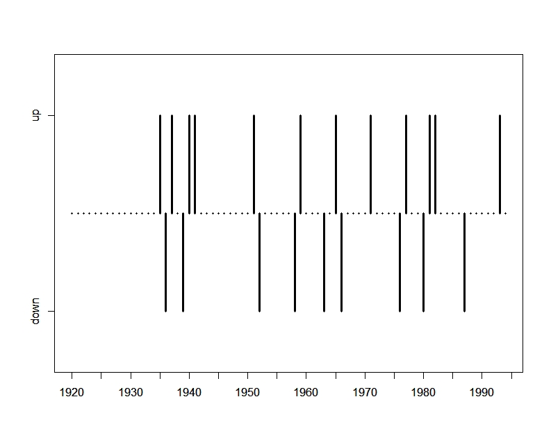
Refer to caption
Figure S1. Map of weather stations (sampling sites) in 6 midwest states.
Refer to caption
Figure S2. Change points detected in every b∈{1,2​…,10}b\in\{1,2\dots,10\}.
Refer to caption Refer to caption
Figure S3. Results of the stepdown procedure for change-point analysis with joint 95% (dark gray) and 99% (gray) confidence intervals of differences of adjacent transformed annual precipitation data from 1920 till 1994. Each figure corresponds to the results of Step 1 with bn=1b_{n}=1 (top left), bn=4b_{n}=4 (top right), bn=7b_{n}=7 (bottom left) and bn=10b_{n}=10 (bottom right).