Unified approach to secondary effects on the CMB B-mode polarization

We begin by introducing the basic idea of the CoS integration approach. The biggest obstacle to treat all nonlinear effects on the evolution of CMB photons in a unified manner is to directly solve their Boltzmann hierarchy: the multipole moments of the CMB anisotropies evolve interdependently in the free-streaming regime, and hence we need to solve a large number of coupled differential equations. At the linear order, this difficulty is resolved by the line-of-sight (LoS) integration approach [53]. In the LoS integration approach, the Boltzmann equation is rewritten in an integral form along a LoS trajectory, i.e. a background photon geodesic. The resultant equation significantly reduces the computational cost. This works successfully because higher multipole moments are not generated dynamically but geometrically in the free-streaming regime: they are generated by the projection of a few multipole moments on a scattering surface to the celestial sphere. The projection is trivial and thus we do not need to solve any equations to know it (see the left panel of figure 1). The LoS integration approach factorizes the observed anisotropies into the factors of this geometrical effect and the collisional effect. Since the geometrical factor is a known quantity, it makes us possible to estimate a large number of observed CMB multipole moments by calculating only a small number of multipole moments in the collision term.

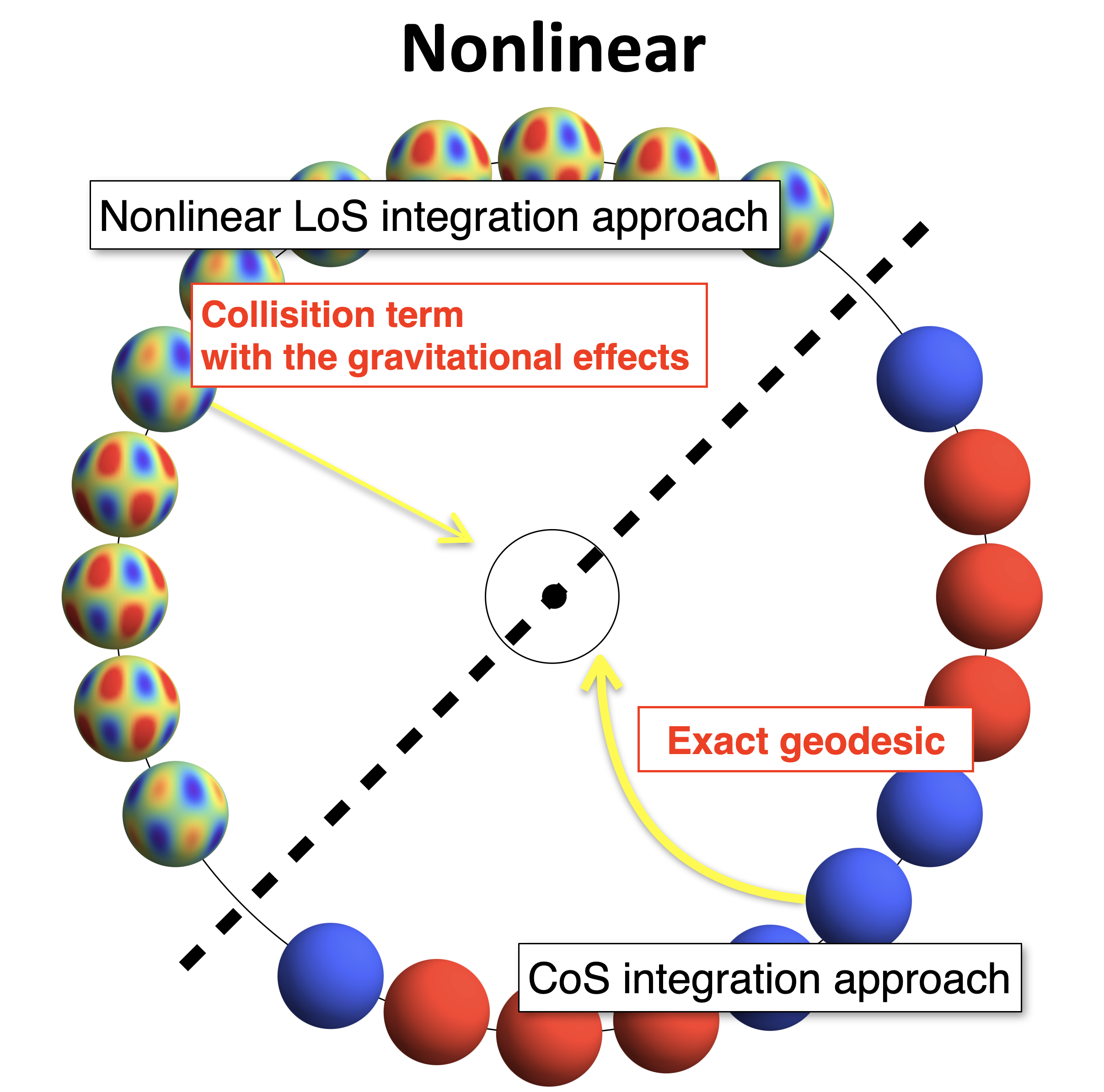
However, its naive extension to the nonlinear order does not work [54, 55]. We will see it explicitly in subsection 2.3, but let us briefly sketch the main difficulty of the extension and why the CoS integration approach resolves it. At the nonlinear order, CMB photons travel in the perturbed spacetime after the last scattering. It distorts the CMB anisotropies and such a distortion can be interpreted as a result of various gravitational effects: lensing, redshift, time delay, and so on. One approach to treat these gravitational effects is to put them into the collision term and rewrite the Boltzmann equation as a LoS integral, i.e. the gravitational effects are interpreted as the scattering of CMB photons (see the nonlinear LoS integration approach in the right panel of figure 1). In this approach, the gravitational collision terms depend on an infinite number of photon multipole moments at each time and thus spoil the success of the LoS integration approach. Because of this difficulty, as we have already mentioned in the introduction, each nonlinear effect has been treated with different approaches in the literature (see, e.g., refs. [47, 48, 49, 51, 54, 55, 57, 37] and the description in ref. [52]). The CoS integration approach is one of the first approaches that can treat all nonlinear effects in a single framework [52] (see ref. [56] for the other approach).

The bottom line of the CoS integration approach is Liouville’s theorem in curved spacetime: in the free-streaming regime, the distribution function is conserved along a geodesic even in the presence of gravity [58]. The theorem says that the evolution of CMB photons after decoupling is determined by solving the geodesic equations instead of the Boltzmann equation. To make use of this theorem, in the CoS integration approach, we rewrite the Boltzmann equation in an integral form along the exact geodesic in the perturbed spacetime. In contrast to the nonlinear LoS integration approach, the gravitational effects now appear in the projection between a scattering surface and the celestial sphere (see the CoS integration approach in the right panel of figure 1). This is not a problem: a perturbed geodesic equation is an ordinary differential equation that can be solved iteratively when a finite number of functions, the metric potentials, are inputted. As an application, it has been shown in ref. [52] that the CoS integration approach gives formulae to calculate the CMB temperature bispectrum generated from the foreground gravitational effects with a less computational cost. Since Liouville’s theorem is also applied to polarized photons, it is expected that the same is true for the CMB polarization. Motivated by these facts, in the following subsections, we will develop the CoS integration approach for the polarization.

We first briefly review how the Boltzmann equation is formulated for polarized photons [59, 60, 61, 35, 45]. The distribution of polarized photons is represented by a tensor-valued function $\hat{f}_{\mu\nu}$ in phase space, whose projection ${\epsilon}^{\mu}[{\epsilon}^{\nu}]^{\ast}\hat{f}_{\mu\nu}$ provides the phase-space number density of photons with polarization ${\epsilon}^{\mu}$. The distribution function $\hat{f}_{\mu\nu}$ is given as a function of the momentum $P^{\mu}$ as well as the spacetime coordinates $x^{\mu}$. The spacetime coordinates are fixed by imposing gauge conditions, but there are still degrees of freedom to choose coordinates in the momentum space [59, 45]. In order to separate the effects of gravity from the local scattering processes of photons, we use the conformal momentum of a photon in a local inertial frame $q^{(\alpha)}$ defined by

$\displaystyle q^{(\alpha)}\equiv a(\eta)\,e^{(\alpha)}{}_{\mu}P^{\mu}\,.$

(2.1)

The quantity $a(\eta)$ is the scale factor of the Friedmann–Lemaître–Robertson–Walker (FLRW) universe at a conformal time $\eta$, $e^{(\alpha)}{}_{\mu}$ is the tetrads and $P^{\mu}$ is the momentum in the coordinate frame. For later convenience, we shall denote its magnitude and direction by

$\displaystyle q\equiv\sqrt{\delta_{(i)(j)}q^{(i)}q^{(j)}}\,,\qquad n^{(i)}\equiv\frac{q^{(i)}}{q}\,,$

(2.2)

and the phase-space coordinates $({\bm{x}},q,{\bm{n}})$ by the symbol ${\bm{z}}$ in short: ${\bm{z}}\equiv({\bm{x}},q,{\bm{n}})$.

The components of $\hat{f}_{\mu\nu}$ do not all describe the physical degrees of freedom but also contain gauge degrees of freedom associated with the longitudinal modes of photons. We can eliminate these gauge degrees of freedom by the projection operator onto the screen orthogonal to the four-velocity of the locally inertial observer $u^{\mu}\equiv e_{(0)}{}^{\mu}$ and the direction of a photon $n^{\mu}\equiv e_{(i)}{}^{\mu}n^{(i)}$, ³³ 3 The screen projector was denoted as $S_{\mu\nu}$ in ref. [52], but we will use a different symbol to avoid confusion with the source function defined in eq. (2.16).

$\displaystyle{\cal H}_{\mu\nu}\equiv g_{\mu\nu}+u_{\mu}u_{\nu}-n_{\mu}n_{\nu}\,.$

(2.3)

Using the projection operator ${\cal H}_{\mu\nu}$, the physical distribution function $f_{\mu\nu}$ is defined by

$\displaystyle f_{\mu\nu}\equiv{\cal H}_{\mu}{}^{\mu^{\prime}}{\cal H}_{\nu}{}^{\nu^{\prime}}\hat{f}_{\mu^{\prime}\nu^{\prime}}\,.$

(2.4)

The polarization basis vectors ${\epsilon_{\sigma}}^{\mu}$ for the two helicity states $\sigma=+,-$ span the screen. Therefore, the screen projector (2.3) can be expanded in terms of them as ⁴⁴ 4 The indices $\rho,\sigma$ of the polarization basis vectors are raised and lowered by $\delta^{\rho\sigma}$ and $\delta_{\rho\sigma}$, respectively.

$\displaystyle{\cal H}_{\mu\nu}=\delta_{\rho\sigma}{\epsilon^{\ast}{}^{\rho}}_{\mu}{\epsilon^{\sigma}}_{\nu}\,,$

(2.5)

and then the physical distribution function (2.4) as

$\displaystyle f_{\mu\nu}=f_{\rho\sigma}{\epsilon^{\ast}{}^{\rho}}_{\mu}{\epsilon^{\sigma}}_{\nu}~.$

(2.6)

The four components $f_{\rho\sigma}$ describe the physical degrees of freedom, which correspond to the Stokes parameters as

$\displaystyle\left(\begin{array}[]{cc}f_{++}&f_{+-}\\ f_{-+}&f_{--}\end{array}\right)=\left(\begin{array}[]{cc}f_{I}-f_{V}&f_{Q}-if_{U}\\ f_{Q}+if_{U}&f+f_{V}\end{array}\right)\,,$

where $f_{I}$ is the intensity, $f_{V}$ the circular polarization, $f_{Q}$ and $f_{U}$ the linear polarization.

In terms of the distribution function for polarized photons $\hat{f}_{\mu\nu}$, the Boltzmann equation is given by

$\displaystyle\frac{\cal D}{{\cal D}\eta}\hat{f}_{\mu\nu}=\dot{\bar{\tau}}\hat{C}_{\mu\nu}\,,$

(2.11)

with the collision term $\dot{\bar{\tau}}\hat{C}_{\mu\nu}$ where the optical depth $\bar{\tau}$ is factorized. ⁵⁵ 5 In contrast to ref. [35], we factorize the optical depth from the definition of the collision term. Moreover, we defined the optical depth in terms of the background electron number density, putting the perturbation in the free electron number density $\delta n_{e}$ to the collision term $\hat{C}_{\mu\nu}$ [52]. This definition makes the optical depth independent of a LoS direction and thus would be more convenient to evaluate the gravitational effects at higher order. However, it is not necessary to care about this technical remark in the estimation in section 5 because $\delta n_{e}$ does not contribute to the linear-order collision term. Here, ${\cal D}/{\cal D}\eta$ denotes the covariant derivative along a photon geodesic $x^{\mu}(\eta)$ in a perturbed spacetime,

$\displaystyle\frac{\cal D}{{\cal D}\eta}\equiv\frac{\mathrm{d}x^{\mu}(\eta)}{\mathrm{d}\eta}\nabla_{\mu}+\frac{\mathrm{d}q^{(i)}(\eta)}{\mathrm{d}\eta}\frac{\partial}{\partial q^{(i)}}\,,$

(2.12)

where $\nabla_{\mu}$ is the covariant derivative of the spacetime. The Boltzmann equation for the physical degrees of freedom $f_{\mu\nu}$ can be obtained by applying ${\cal D}/{\cal D}\eta$ to $f_{\mu\nu}\equiv{\cal H}_{\mu}{}^{\mu^{\prime}}{\cal H}_{\nu}{}^{\nu^{\prime}}\hat{f}_{\mu^{\prime}\nu^{\prime}}$,

$\displaystyle{\cal H}_{\mu}{}^{\mu^{\prime}}{\cal H}_{\nu}{}^{\nu^{\prime}}\frac{\cal D}{{\cal D}\eta}f_{\mu^{\prime}\nu^{\prime}}=\dot{\bar{\tau}}C_{\mu\nu}\,,$

(2.13)

where $C_{\mu\nu}\equiv{\cal H}_{\mu}{}^{\mu^{\prime}}{\cal H}_{\nu}{}^{\nu^{\prime}}\hat{C}_{\mu^{\prime}\nu^{\prime}}$. Here, we have used the geodesic equation and the fact that ${\cal H}_{\mu\nu}\,,\hat{f}_{\mu\nu}$ are orthogonal to $P^{\mu}$. The latter equation (2.13) has been usually used for nonlinear analysis of the Boltzmann equation, but we start with the former equation (2.11) to develop the CoS integration approach in next subsection. This is because the screen projector ${\cal H}_{\mu}{}^{\mu^{\prime}}$ does not commute with the parallel transport operator and makes the argument cumbersome.

Based on the basic idea in subsection 2.1, we rewrite the Boltzmann equation (2.11) to an integral equation along a geodesic (see also ref. [62] for an earlier work on the integral formulation for polarized photons).

In the CoS integration approach, the integration is performed along an exact geodesic. Before formulating it, let us first see why the nonlinear LoS integration approach in figure 1 does not work, i.e. what difficulty arises when the integration is performed along a background geodesic at the nonlinear order. In the nonlinear LoS integration approach, the Liouville term ${\cal D}\hat{f}_{\mu\nu}/{\cal D}\eta$ is separated as

$\displaystyle\frac{{\cal D}\hat{f}_{\mu\nu}}{{\cal D}\eta}=\frac{{\cal\bar{D}}\hat{f}_{\mu\nu}}{{\cal\bar{D}}\eta}+\hat{\cal M}_{\mu\nu}\,,$

(2.14)

where the derivative ${\cal\bar{D}}/{\cal\bar{D}}\eta$ is defined for a background geodesic $\bar{\bm{z}}(\eta)$ and $\hat{\cal M}_{\mu\nu}$ represents terms containing the geodesic perturbations, i.e. the difference between a background and full geodesic $\delta{\bm{z}}(\eta)\equiv{\bm{z}}(\eta)-\bar{\bm{z}}(\eta)$. Then, we rewrite the Boltzmann equation in an integral form as

$\displaystyle\hat{f}_{\mu\nu}(\eta_{0},{\bm{z}}_{0})=\int_{0}^{\eta_{0}}{\rm d}\eta_{s}~\left\{\bar{g}_{v}(\eta_{s})\hat{S}_{\mu\nu}\left[\eta_{s},\bar{\bm{z}}(\eta_{s};\eta_{0},{\bm{z}}_{0})\right]-e^{-\bar{\tau}(\eta_{s})}\hat{\cal M}_{\mu\nu}\left[\eta_{s},\bar{\bm{z}}(\eta_{s};\eta_{0},{\bm{z}}_{0})\right]\right\}\,,$

(2.15)

for the distribution function at present $\eta=\eta_{0}$, introducing the visibility function $\bar{g}_{v}$ and the source function $\hat{S}_{\mu\nu}$ by

$\displaystyle\bar{g}_{v}\equiv-\dot{\bar{\tau}}e^{-\bar{\tau}}\,,\quad\hat{S}_{\mu\nu}\equiv\hat{f}_{\mu\nu}-\hat{C}_{\mu\nu}\,.$

(2.16)

Here, $\bar{\bm{z}}(\eta_{s};\eta_{0},{\bm{z}}_{0})$ in the integrand denotes the phase-space coordinates ${\bm{z}}=({\bm{x}},q,{\bm{n}})$ on the background geodesic that give the observed data ${\bm{z}}_{0}=({\bm{x}}_{0},q_{0},{\bm{n}}_{0})$ at present $\eta_{s}=\eta_{0}$, i.e. $\bar{\bm{z}}(\eta_{s};\eta_{0},{\bm{z}}_{0})|_{\eta_{s}=\eta_{0}}={\bm{z}}_{0}$. The foreground gravitational effects are included in the term $\hat{\cal M}_{\mu\nu}$: the perturbations in the ${\rm d}x^{i}/{\rm d}\eta$ term of eq. (2.12) give the lensing and time-delay effects, and the perturbations in the ${\rm d}q^{(i)}/{\rm d}\eta$ term give the redshift and emission-angle effects. At the linear order, it only contains the redshift term:

$\displaystyle\left.\hat{\cal M}_{\mu\nu}\right|^{\mathrm{linear}}=\frac{\mathrm{d}[\delta q(\eta)]}{\mathrm{d}\eta}\frac{\partial{\bar{f}}_{\mu\nu}}{\partial q}\,,$

(2.17)

which corresponds to the well-known Sachs-Wolfe (SW) and integrated Sachs-Wolfe (ISW) effects. Here, $\bar{f}_{\mu\nu}$ is the background counterpart of $\hat{f}_{\mu\nu}$. In order that the LoS integration formula (2.15) successfully works, the source function $\hat{S}_{\mu\nu}$ should depend only on a small number of multipole moments of the distribution function $\hat{f}_{\mu\nu}$ (see the left panel of figure 1). This is true for the linear-order $\hat{\cal M}_{\mu\nu}$ term (2.17) but not for the nonlinear order term: the $\hat{\cal M}_{\mu\nu}$ term depends on $\hat{f}_{\mu\nu}$, instead of $\bar{f}_{\mu\nu}$ in the linear case (2.17), and thus an infinite number of its multipole moments.

On the other hand, in the CoS integration approach, the Boltzmann equation (2.11) is rewritten in an integral form along an exact geodesic in the perturbed spacetime, ${\bm{z}}(\eta_{s};\eta_{0},{\bm{z}}_{0})$, instead of its background counterpart $\bar{\bm{z}}(\eta_{s};\eta_{0},{\bm{z}}_{0})$ in the LoS integration approach (2.15) (see figure 2). To formulate it for polarized photons, we first introduce a parallel-transport operator along an exact geodesic $x^{\mu}(\eta_{s};\eta_{0},{\bm{z}}_{0})$ from a source to the observer, ${\cal P}_{\mu_{0}}{}^{\mu_{s}}$, which satisfies the differential equation

$\displaystyle\frac{\mathrm{d}{\cal P}_{\mu_{0}}{}^{\mu_{s}}}{\mathrm{d}\eta_{s}}=-\Gamma^{\mu_{s}}{}_{\mu\nu}{\cal P}_{\mu_{0}}{}^{\mu}\frac{\mathrm{d}x^{\nu}(\eta_{s})}{\mathrm{d}\eta_{s}}\,,$

(2.18)

and ${\cal P}_{\mu_{0}}{}^{\mu_{s}}=\delta_{\mu_{0}}^{\mu_{s}}$ at $\eta_{s}=\eta_{0}$. Here, $\Gamma^{\mu_{s}}{}_{\mu\nu}$ is the connection in the perturbed spacetime. In terms of the parallel-transport operator ${\cal P}_{\mu_{0}}{}^{\mu_{s}}$, we define the tensor-valued function at the observer’s position,

$\displaystyle\left({\cal P}\hat{f}\right)_{\mu_{0}\nu_{0}}(\eta_{s};\eta_{0},{\bm{z}}_{0})\equiv\left.{\cal P}_{\mu_{0}}{}^{\mu_{s}}{\cal P}_{\nu_{0}}{}^{\nu_{s}}\hat{f}_{\mu_{s}\nu_{s}}(\eta_{s},{\bm{z}})\right|_{{\bm{z}}={\bm{z}}(\eta_{s};\eta_{0},{\bm{z}}_{0})}\,,$

(2.19)

with $\eta_{s}$ being treated as a parameter. This function satisfies the following ordinary differential equation,

$\displaystyle\frac{\mathrm{d}}{\mathrm{d}\eta_{s}}\left({\cal P}\hat{f}\right)_{\mu_{0}\nu_{0}}(\eta_{s};\eta_{0},{\bm{z}}_{0})={\cal P}_{\mu_{0}}{}^{\mu_{s}}{\cal P}_{\nu_{0}}{}^{\nu_{s}}\frac{{\cal D}\hat{f}_{\mu_{s}\nu_{s}}}{{\cal D}\eta_{s}}\,,$

(2.20)

as well as the condition $({\cal P}\hat{f})_{\mu_{0}\nu_{0}}(\eta_{s};\eta_{0},{\bm{z}}_{0})|_{\eta_{s}=\eta_{0}}=\hat{f}_{\mu_{0}\nu_{0}}(\eta_{0},{\bm{z}}_{0})$. Therefore, the Boltzmann equation (2.11) can be rewritten as

$\displaystyle\frac{\mathrm{d}}{\mathrm{d}\eta_{s}}\left({\cal P}\hat{f}\right)_{\mu_{0}\nu_{0}}=\dot{\bar{\tau}}{\cal P}_{\mu_{0}}{}^{\mu_{s}}{\cal P}_{\nu_{0}}{}^{\nu_{s}}\hat{C}_{\mu_{s}\nu_{s}}\,,$

(2.21)

and then formally integrated as

$\displaystyle\hat{f}_{\mu_{0}\nu_{0}}(\eta_{0},{\bm{z}}_{0})=\int_{0}^{\eta_{0}}{\rm d}\eta_{s}~\bar{g}_{v}(\eta_{s}){\cal P}_{\mu_{0}}{}^{\mu_{s}}{\cal P}_{\nu_{0}}{}^{\nu_{s}}\hat{S}_{\mu_{s}\nu_{s}}\left[\eta_{s},{\bm{z}}(\eta_{s};\eta_{0},{\bm{z}}_{0})\right]\,.$

(2.22)

In contrast to the LoS integral (2.15), the gravitational term $\hat{\cal M}_{\mu\nu}$ does not appear in the integrand. Instead, the gravitational effects appear in the evaluation point of the source term: $\hat{S}_{\mu\nu}\left[\eta_{s},\bar{\bm{z}}(\eta_{s};\eta_{0},{\bm{z}}_{0})\right]\to\hat{S}_{\mu\nu}\left[\eta_{s},{\bm{z}}(\eta_{s};\eta_{0},{\bm{z}}_{0})\right]$. It is illustrated in figure 2 how the evaluation point of the source term is determined for a given observed data ${\bm{z}}_{0}$ in the nonlinear LoS and CoS integration approaches (see also figure 1 for the difference of the two approaches). As mentioned before, in the nonlinear LoS integration approach (2.15), it is necessary to integrate a large number of multipole moments along a background geodesic $\bar{\bm{z}}(\eta_{s};\eta_{0},{\bm{z}}_{0})$. On the other hand, in the CoS integration approach (2.22), the observed distribution can be computed by integrating a small number of multipole moments along an exact geodesic ${\bm{z}}(\eta_{s};\eta_{0},{\bm{z}}_{0})$. Since the exact geodesic can be determined by solving the geodesic equations, it is not necessary to solve the Boltzmann hierarchy for a large number of multipole moments.

In the remaining part of this subsection, we will further rewrite the CoS formula (2.22) in terms of the distribution function for physical degrees of freedom, $f_{\rho\sigma}$, introduced in eq. (2.4). It can be achieved by projecting $\hat{f}_{\mu\nu}(\eta_{0},{\bm{z}}_{0})$ on the screen at the observer’s position, which is spanned by the two polarization basis vectors ${\epsilon_{\sigma_{0}}}^{\mu_{0}}(\eta_{0},{\bm{z}}_{0})$:

$\displaystyle f_{\rho_{0}\sigma_{0}}(\eta_{0},{\bm{z}}_{0})={\epsilon_{\rho_{0}}}^{\mu_{0}}(\eta_{0},{\bm{z}}_{0}){\epsilon^{\ast}{}_{\sigma_{0}}}^{\mu_{0}}(\eta_{0},{\bm{z}}_{0})\hat{f}_{\mu_{0}\nu_{0}}(\eta_{0},{\bm{z}}_{0})\,,$

(2.23)

and hence,

$\displaystyle f_{\rho_{0}\sigma_{0}}(\eta_{0},{\bm{z}}_{0})$

$\displaystyle=\int_{0}^{\eta_{0}}{\rm d}\eta_{s}~\bar{g}_{v}(\eta_{s})\left[{\epsilon_{\rho_{0}}}^{\mu_{0}}{\cal P}_{\mu_{0}}{}^{\mu_{s}}\right]\left[{\epsilon_{\sigma_{0}}}^{\nu_{0}}{\cal P}_{\nu_{0}}{}^{\nu_{s}}\right]^{\ast}\hat{S}_{\mu_{s}\nu_{s}}\left[\eta_{s},{\bm{z}}(\eta_{s};\eta_{0},{\bm{z}}_{0})\right]\,,$

(2.24)

where we have suppressed the arguments of the polarization basis vectors in the integrand for brevity. In eq. (2.24), ${\epsilon_{\rho_{0}}}^{\mu_{0}}{\cal P}_{\mu_{0}}{}^{\mu_{s}}$ is a vector orthogonal to the four-momentum $P^{\mu_{s}}$ at $\eta=\eta_{s}$. Hence, it can be expanded in terms of ${\epsilon_{\rho_{s}}}^{\mu_{s}}$ and $P^{\mu_{s}}$ as

$\displaystyle{\epsilon_{\rho_{0}}}^{\mu_{0}}{\cal P}_{\mu_{0}}{}^{\mu_{s}}=U_{\rho_{0}}{}^{\rho_{s}}{\epsilon_{\rho_{s}}}^{\mu_{s}}+\alpha_{\rho_{0}}(\eta_{s})P^{\mu_{s}}\,,$

(2.25)

using a unitary matrix $U_{\rho_{0}}{}^{\rho_{s}}$. Here, the last term should be added because the time direction $e_{(0)}{}^{\mu}$ does not satisfy the parallel transport equation; the coefficient $\alpha_{\rho_{0}}(\eta_{s})$ is determined so that the vector ${\epsilon_{\rho_{0}}}^{\mu_{0}}{\cal P}_{\mu_{0}}{}^{\mu_{s}}-\alpha_{\rho_{0}}(\eta_{s})P^{\mu_{s}}$ is orthogonal to $e_{(0)}{}^{\mu_{s}}(\eta_{s})$ but the final result does not depend on its value because the source term satisfies $P^{\mu_{s}}\hat{S}_{\mu_{s}\nu_{s}}=0$. The unitary matrix $U_{\rho_{0}}{}^{\rho_{s}}$ is a diagonal matrix in the helicity basis as

$\displaystyle\left(\begin{matrix}U_{+}{}^{+}&U_{+}{}^{-}\\ U_{-}{}^{+}&U_{-}{}^{-}\\ \end{matrix}\right)=\left(\begin{matrix}e^{i\psi}&0\\ 0&e^{-i\psi}\\ \end{matrix}\right)\,,$

(2.26)

where $\psi$ describes the rotation of the helicity basis.

In conclusion, the distribution function is written only in terms of physical degrees of freedom (i.e. projected quantities) as

$\displaystyle f_{\rho_{0}\sigma_{0}}(\eta_{0},{\bm{z}}_{0})$

$\displaystyle=\int_{0}^{\eta_{0}}{\rm d}\eta_{s}~\bar{g}_{v}(\eta_{s})~U_{\rho_{0}}{}^{\rho_{s}}\bigl[U_{\sigma_{0}}{}^{\sigma_{s}}\bigr]^{\ast}S_{\rho_{s}\sigma_{s}}\left[\eta_{s},{\bm{z}}(\eta_{s};\eta_{0},{\bm{z}}_{0})\right]\,,$

(2.27)

where

$\displaystyle S_{\rho_{s}\sigma_{s}}\left[\eta_{s},{\bm{z}}(\eta_{s};\eta_{0},{\bm{z}}_{0})\right]\equiv{\epsilon_{\rho_{s}}}^{\mu_{s}}{\epsilon^{\ast}{}_{\sigma_{s}}}^{\nu_{s}}\hat{S}_{\mu_{s}\nu_{s}}\left[\eta_{s},{\bm{z}}(\eta_{s};\eta_{0},{\bm{z}}_{0})\right]\,,$

(2.28)

is the source term for the physical degrees of freedom. The projected source term (2.28) has been calculated up to the second order in the perturbations in ref. [35].

Instead of treating the full $q$-dependence in eq. (2.27), we use the brightness of polarized photons taking the third moment of the distribution function, ⁶⁶ 6 At the nonlinear order, Compton collisions at recombination and during the reionization era induces deviations from a blackbody spectrum [44, 45, 46, 63, 64, 65, 66, 67, 68]. The spectral distortion can be treated by the CoS formula for the distribution function (2.27). We leave it for future work to treat the spectral distortion and will concentrate on showing how the foreground gravitational effects are integrated into the direct Boltzmann-equation approach.

$\displaystyle\delta_{\rho\sigma}+\Delta_{\rho\sigma}\equiv\frac{2}{\bar{B}}\left(\int\!{\rm d}q~q^{3}~f_{\rho\sigma}\right)\,;\quad\bar{B}\equiv\int\!{\rm d}q~q^{3}~{\rm tr}(\bar{f}_{\bar{\rho}\bar{\sigma}})\,,$

(2.29)

where the four components of $\Delta_{\rho\sigma}$ can be decomposed as

$\displaystyle\left(\begin{array}[]{cc}\Delta_{++}&\Delta_{+-}\\ \Delta_{-+}&\Delta_{--}\end{array}\right)=\left(\begin{array}[]{cc}\Delta-\Delta_{V}&\Delta_{Q}-i\Delta_{U}\\ \Delta_{Q}+i\Delta_{U}&\Delta+\Delta_{V}\end{array}\right)~,$

like the distribution function in eq. (2.2). Then, integrating eq. (2.27) for $q_{0}$, we obtain a formula

$\displaystyle\delta_{\rho_{0}\sigma_{0}}+\Delta_{\rho_{0}\sigma_{0}}(\eta_{0},{\bm{x}}_{0},{\bm{n}}_{0})$

$\displaystyle=\int_{0}^{\eta_{0}}{\rm d}\eta_{s}~\bar{g}_{v}(\eta_{s})\,e^{-4\delta\ln q(\eta_{s})}U_{\rho_{0}}{}^{\rho_{s}}\bigl[U_{\sigma_{0}}{}^{\sigma_{s}}\bigr]^{\ast}\Xi_{\rho_{s}\sigma_{s}}\left[\eta_{s},{\bm{x}}(\eta_{s}),{\bm{n}}(\eta_{s})\right]\,,$

(2.34)

where we have defined,

$\displaystyle\Xi_{\rho_{s}\sigma_{s}}\equiv\frac{2}{\bar{B}}\left(\int\!{\rm d}q~q^{3}S_{\rho_{s}\sigma_{s}}\right)\,,$

(2.35)

and $\delta\ln q(\eta_{s})\equiv\ln q(\eta_{s})-\ln q_{0}$. Here, the functions ${\bm{x}}(\eta_{s})$, ${\bm{n}}(\eta_{s})$ are the components of ${\bm{z}}(\eta_{s};\eta_{0},{\bm{z}}_{0})$, and satisfy ${\bm{x}}(\eta_{0})={\bm{x}}_{0}$ and ${\bm{n}}(\eta_{0})={\bm{n}}_{0}$, respectively. In the derivation, we have used the fact that ${\bm{x}}(\eta_{s})$, ${\bm{n}}(\eta_{s})$, $\delta\ln q(\eta_{s})$, and $U_{\rho_{0}}{}^{\rho_{s}}$ do not depend on $q_{0}$ (see Appendix E).

The formula (2.34) is one of the main results in this paper. It is an extension of the curve-of-sight (CoS) integration approach [52] to the CMB polarization. The trace of eq. (2.34) reproduces the result in ref. [52] for the intensity. As we have mentioned below eq. (2.22) for the distribution function, once the perturbed geodesic is determined by solving the geodesic equations, this formula enables us to compute the observed brightness $\Delta_{\rho_{0}\sigma_{0}}$ without solving the Boltzmann hierarchy for a large number of multipole moments. This can be seen clearly when the Fourier transformation and multipole expansion of the source function $\Xi_{\rho_{s}\sigma_{s}}$ are performed. Taking the intensity as an example, its source function can be expanded as

$\displaystyle\Xi[\eta_{s},{\bm{x}},{\bm{n}}]=\sum_{\ell m}N_{\ell}\int\frac{\mathrm{d}^{3}{\bm{k}}}{(2\pi)^{3}}~\Xi_{\ell m}(\eta_{s},{\bm{k}})\,Y_{\ell m}({\bm{n}})e^{i{\bm{k}}\cdot{\bm{x}}}\,,$

(2.36)

where $N_{\ell}$ is a numerical coefficient. Note that this expansion is defined on a scattering surface $\eta=\eta_{s}$ and irrelevant to any information at $\eta>\eta_{s}$. Therefore, the structure of the expansion does not depend on whether the spacetime is perturbed or not at $\eta>\eta_{s}$. For the Compton scattering, only a few multiple moments of $\Xi_{\ell m}(\eta,{\bm{k}})$ are nonzero and thus the summation for $\ell,m$ contains few terms in eq. (2.36). In the CoS formula (2.34), the observed brightness $\Delta(\eta_{0},{\bm{x}}_{0},{\bm{n}}_{0})$ can be computed by evaluating the source term $\Xi[\eta_{s},{\bm{x}},{\bm{n}}]$ on an exact geodesic $({\bm{x}},{\bm{n}})=({\bm{x}}(\eta_{s}),{\bm{n}}(\eta_{s}))$. The foreground gravitational effects appear as deviations in the evaluation point: $(\bar{\bm{x}}(\eta_{s}),\bar{\bm{n}}(\eta_{s}))\to({\bm{x}}(\eta_{s}),{\bm{n}}(\eta_{s}))$. In the expanded form (2.36), the dependence on ${\bm{x}}$ and ${\bm{n}}$ are represented by the geometrical factor $Y_{\ell m}({\bm{n}})e^{i{\bm{k}}\cdot{\bm{x}}}$, which is a known function of ${\bm{x}}$ and ${\bm{n}}$. Therefore, we can determine all the multipole moments of the observed brightness $\Delta_{\ell m}$ by calculating a finite number of functions $\Xi_{\ell m}(\eta_{s},{\bm{k}})$, $\ln q(\eta_{s})$, ${\bm{x}}(\eta_{s})$, ${\bm{n}}(\eta_{s})$: it is not necessary to solve a thousand of coupled differential equations. Here, we have explained how the CoS formula (2.34) reduces the computational cost for the intensity, but the same argument holds for the polarization: the source function can be expanded as

$\displaystyle\Xi_{\pm\mp}[\eta_{s},{\bm{x}},{\bm{n}}]=\sum_{\ell m}N_{\ell}\int\frac{\mathrm{d}^{3}{\bm{k}}}{(2\pi)^{3}}~\Xi_{\ell m}(\eta_{s},{\bm{k}})\,{}_{\pm 2}Y_{\ell m}({\bm{n}})e^{i{\bm{k}}\cdot{\bm{x}}}\,,$

(2.37)

where the spin-weighted spherical harmonics ${}_{s}Y_{\ell m}({\bm{n}})$ appears instead of the usual spherical harmonics $Y_{\ell m}({\bm{n}})$ in eq. (2.36). In contrast to the usual spherical harmonics $Y_{\ell m}({\bm{n}})$, the spin-weighted spherical harmonics ${}_{s}Y_{\ell m}({\bm{n}})$ depends on the polarization basis vectors ${\epsilon_{\sigma_{s}}}^{\mu_{s}}(\eta_{s},{\bm{x}},{\bm{n}})$ (see Appendix B). This does not spoil the argument above: we can arbitrarily choose the polarization basis vectors ${\epsilon_{\sigma_{s}}}^{\mu_{s}}(\eta_{s},{\bm{x}},{\bm{n}})$ at each point in the phase space. For a given choice of the polarization basis vectors, they are written in terms of known functions of ${\bm{x}}$ and ${\bm{n}}$ (see subsection 3.1 and Appendix A for details on our choice). Therefore, the observed brightness $\Delta_{\pm,\mp}$ can be still determined by calculating a finite number of functions $\Xi_{\ell m}(\eta_{s},{\bm{k}})$, $\ln q(\eta_{s})$, ${\bm{x}}(\eta_{s})$, and ${\bm{n}}(\eta_{s})$. Because the CoS formula (2.34) is derived from the Boltzmann equation without any approximation, it gives a way to evaluate the correlation functions with arbitrarily high accuracy. It can treat all the foreground gravitational effects without encountering the difficulty of the Boltzmann hierarchy. It is also noted that the thin-screen approximation is not invoked to derive the formula (2.34). Therefore, the CoS formula (2.34) can treat extended sources such as the contributions after the reionization.

In this subsection, we first address the issue in the step (i): we define the perturbation of the source function $\Xi_{\rho_{s}\sigma_{s}}$ at each point in the phase space. In the standard treatment of the perturbation theory, background and perturbed quantities in spacetime are compared at points with the same coordinate values and for the same components in the spacetime coordinate basis. Since the source function $\Xi_{\rho_{s}\sigma_{s}}$ is a tensor on the screen at a phase-space point, in a similar manner, we define its perturbation as the difference between the background and perturbed source functions at points with the same coordinate values in the phase space $(x^{i_{s}},n^{(i_{s})})$ and for the same components in the polarization basis ${\epsilon_{\sigma_{s}}}^{\mu_{s}}$ [45]. In this definition, the perturbation of the source function $\Xi_{\rho_{s}\sigma_{s}}$ depends on the choice of the polarization basis vectors ${\epsilon_{\sigma_{s}}}^{\mu_{s}}$ in the perturbed phase space, as the gauge transformation is induced when the coordinates of the perturbed spacetime are changed. Although the observed quantities do not depend on the choice of the polarization basis vectors ${\epsilon_{\sigma_{s}}}^{\mu_{s}}$ at the emission point, we will show that there is a convenient choice for the calculation in the CoS integration approach. ⁷⁷ 7 Different results for the polarization-rotation effect are found in the literature (e.g., refs. [48, 49, 50, 51]). This is due to different choices of the polarization basis vectors.

The polarization basis vectors can be arbitrarily chosen at each point in the phase space. We would like to choose them so that the calculations in the CoS integration approach become simple. For example, one can define the polarization basis vectors by the parallel transport from the observer’s position. For this choice, it is clear from its definition that the polarization-rotation angle $\psi$ identically vanishes (see eq. (2.25)). However, we do not choose this basis because information of the foreground spacetime is involved in the source term and thus in the local expansion (2.37). Among various possible choices, we choose the rigid basis: the polarization basis vectors are defined by the polar and azimuthal directions in the tetrad frame at each point [35] (see Appendix A for more details). In the rigid basis, the polarization basis vectors do not depend on the spacetime coordinates but only on the momentum in a local inertial frame, i.e. ${\epsilon_{\pm}}^{(i)}={\epsilon_{\pm}}^{(i)}({\bm{n}})$. In figure 4, we have illustrated how the background and perturbed ${\bm{n}}$-spaces are identified to define the perturbation when the rigid basis or general basis is chosen. In the following, we will also use the vector notation ${\bm{\epsilon}}_{\pm}$ for ${\epsilon_{\pm}}^{(i)}$.

The reason for this specific choice is that the spin-weighted spherical harmonics ${}_{s}Y_{\ell m}$ becomes independent of ${\bm{x}}$ in the rigid basis. One can check this fact by using the explicit expressions of the rigid basis and spin-weighted spherical harmonics in Appendix A and B. On the other hand, when the polarization basis vectors are changed as ${\bm{\epsilon}}_{\pm}\to e^{\pm i\gamma({\bm{x}})}{\bm{\epsilon}}_{\pm}$ from the rigid basis ($\gamma({\bm{x}})$ is an arbitrary function of ${\bm{x}}$), this leads to a rearrangement between the polarization-rotation matrix and the source function as

		$\displaystyle U_{\pm}{}^{\pm}(\eta)\to U^{(\gamma)}{}_{\pm}{}^{\pm}\equiv U_{\pm}{}^{\pm}(\eta)e^{\pm i\Delta\gamma}\quad(\text{i.e.~}\psi\to\psi+\Delta\gamma)\,,$		(3.3)
		$\displaystyle\Xi_{\pm\mp}\to\Xi^{(\gamma)}{}_{\pm\mp}\equiv\Xi_{\pm\mp}e^{\pm 2i\gamma({\bm{x}})}\,,$		(3.4)

with $\Delta\gamma\equiv\gamma({\bm{x}}_{0})-\gamma({\bm{x}})$ (see eqs. (2.25) and (2.26)). The definition of the spin-weighted spherical harmonics is also changed as

$\displaystyle{}_{s}Y_{\ell m}\to{}_{s}Y^{(\gamma)}_{\ell m}\equiv{}_{s}Y_{\ell m}e^{\pm is\gamma({\bm{x}})}\,,$

(3.5)

and hence ${}_{s}Y_{\ell m}$ in the new basis depends on ${\bm{x}}$: ${}_{s}Y^{(\gamma)}_{\ell m}={}_{s}Y^{(\gamma)}_{\ell m}({\bm{x}},{\bm{n}})$. It is noted that we can make $\psi=0$ with this degree of freedom. As already mentioned above, this is the case when the polarization basis vectors are defined through the parallel transport from the observer’s position. A price to pay is that the source term involves the foreground gravitational effects as well as the ${\bm{x}}$-dependent ${}_{s}Y_{\ell m}$.

The ${\bm{x}}$-dependent ${}_{s}Y_{\ell m}$ causes several technical difficulties in the CoS integration approach. To see it, let us first remind that we need to take the multipole expansion on different spheres in the CoS integration approach: the local expansion (2.37) is performed on a sphere spanned by ${\bm{n}}$ (${\bm{n}}$ sphere) at each emission position $E$, while the observed multipoles are defined on the celestial sphere spanned by ${\bm{n}}_{0}$ (${\bm{n}}_{0}$ sphere) at the observer’s position $O$ (see figure 3). When ${}_{s}Y_{\ell m}$ depends on ${\bm{x}}$, its expression is different for every ${\bm{n}}$ spheres and the celestial sphere (${\bm{n}}_{0}$ sphere). This makes it complicated to relate the multipole expansions at different positions, $O$, $E$, and $\bar{E}$. Moreover, when the definition of ${}_{s}Y_{\ell m}$ is spatially inhomogeneous on the constant-time hypersurface $\eta=\eta_{s}$, it introduces an artificial mode mixing in the Fourier transform (2.37). To circumvent these difficulties, we use the rigid basis in formulating the CoS integration approach. ⁸⁸ 8 It would be also remarkable that the geometrical factor in eq. (2.37) is factorized into the ${\bm{n}}$-dependent factor ${}_{s}Y_{\ell m}({\bm{n}})$ and the ${\bm{x}}$-dependent factor $e^{i{\bm{k}}\cdot{\bm{x}}}$ in the rigid basis. As we will explain in section 4, the displacement $\delta{\bm{x}}(\eta)$ gives the dominant contribution to the lensing. Thus, the higher-order terms and non-Gaussian statistics of $\delta{\bm{x}}(\eta)$ mostly represent the higher-order lensing effects including the nonlinear evolution of the gravitational potential [1] and the post-Born corrections [29, 30, 31, 32, 33, 34]. Since the ${\bm{x}}$ dependence is solely represented by the exponential factor $e^{i{\bm{k}}\cdot{\bm{x}}}$, the rigid basis would be also convenient to handle these higher-order effects.

Provided the definition of the intrinsic (non-gravitational) perturbation of the source function $\Xi_{\rho_{s}\sigma_{s}}$ at each point $({\bm{x}},{\bm{n}})$ in the phase space, we address the issue in the step (ii) to incorporate the foreground gravitational effects. As already mentioned, the foreground gravitational effects can be estimated by comparing the exact brightness (2.34) and the unlensed brightness (3.1) (see figure 3). To compute it, we need to compare the source function $\Xi_{\rho_{s}\sigma_{s}}$ between the background and perturbed emission points, $(\bar{\bm{x}}(\eta_{s}),\bar{\bm{n}}(\eta_{s}))$ and $({\bm{x}}(\eta_{s}),{\bm{n}}(\eta_{s}))$. Their differences depend on how we transport the tensor $\Xi_{\rho_{s}\sigma_{s}}$ from $(\bar{\bm{x}}(\eta_{s}),\bar{\bm{n}}(\eta_{s}))$ to $({\bm{x}}(\eta_{s}),{\bm{n}}(\eta_{s}))$: the path of the transportation and the connection on the bundle of screens. In this subsection, we first define the transportation from $(\bar{\bm{x}}(\eta_{s}),\bar{\bm{n}}(\eta_{s}))$ to $({\bm{x}}(\eta_{s}),{\bm{n}}(\eta_{s}))$ so that the computation of the difference of $\Xi_{\rho_{s}\sigma_{s}}$ between the background and perturbed emission points becomes simple. Expanding the difference with respect to $\delta{\bm{x}}\,,\delta{\bm{n}}$, then, we will express the brightness (2.34) as a series expansion for the geodesic perturbations: eq. (3.30). As in the remapping approach, we can perturbatively estimate the power spectra from the formula (3.30).

References

- [1] A. Lewis and A. Challinor, Weak gravitational lensing of the CMB, Phys. Rept. 429 (2006) 1 [astro-ph/0601594].
- [2] V. Perlick, Gravitational lensing from a spacetime perspective, Living Rev. Rel. 7 (2004) 9.
- [3] M. Bartelmann and P. Schneider, Weak gravitational lensing, Phys. Rept. 340 (2001) 291 [astro-ph/9912508].
- [4] B. D. Sherwin et al., Two-season Atacama Cosmology Telescope polarimeter lensing power spectrum, Phys. Rev. D 95 (2017) 123529 [1611.09753].
- [5] BICEP2, Keck Array collaboration, BICEP2 / Keck Array VIII: Measurement of gravitational lensing from large-scale B-mode polarization, Astrophys. J. 833 (2016) 228 [1606.01968].
- [6] Planck collaboration, Planck 2018 results. VI. Cosmological parameters, Astron. Astrophys. 641 (2020) A6 [1807.06209].
- [7] POLARBEAR collaboration, Measurement of the Cosmic Microwave Background Polarization Lensing Power Spectrum from Two Years of POLARBEAR Data, 1911.10980.
- [8] W. Wu et al., A Measurement of the Cosmic Microwave Background Lensing Potential and Power Spectrum from 500 deg2 of SPTpol Temperature and Polarization Data, Astrophys. J. 884 (2019) 70 [1905.05777].
- [9] M. Kamionkowski, A. Kosowsky and A. Stebbins, A Probe of primordial gravity waves and vorticity, Phys. Rev. Lett. 78 (1997) 2058 [astro-ph/9609132].
- [10] CMB-S4 Science Case, Reference Design, and Project Plan, 2019.
- [11] M. Hazumi et al., LiteBIRD: A Satellite for the Studies of B-Mode Polarization and Inflation from Cosmic Background Radiation Detection, J. Low. Temp. Phys. 194 (2019) 443.
- [12] NASA PICO collaboration, PICO: Probe of Inflation and Cosmic Origins, 1902.10541.
- [13] N. Sehgal et al., CMB-HD: An Ultra-Deep, High-Resolution Millimeter-Wave Survey Over Half the Sky, 1906.10134.
- [14] U. Seljak and C. M. Hirata, Gravitational lensing as a contaminant of the gravity wave signal in CMB, Phys. Rev. D69 (2004) 043005 [astro-ph/0310163].
- [15] K. M. Smith, D. Hanson, M. LoVerde, C. M. Hirata and O. Zahn, Delensing CMB Polarization with External Datasets, JCAP 1206 (2012) 014 [1010.0048].
- [16] T. Namikawa and R. Nagata, Non-Gaussian Structure of B-mode Polarization after Delensing, JCAP 1510 (2015) 004 [1506.09209].
- [17] T. Namikawa, D. Yamauchi, B. Sherwin and R. Nagata, Delensing Cosmic Microwave Background B-modes with the Square Kilometre Array Radio Continuum Survey, Phys. Rev. D93 (2016) 043527 [1511.04653].
- [18] S. Dodelson, E. Rozo and A. Stebbins, Primordial gravity waves and weak lensing, Phys. Rev. Lett. 91 (2003) 021301 [astro-ph/0301177].
- [19] A. Cooray, M. Kamionkowski and R. R. Caldwell, Cosmic shear of the microwave background: The Curl diagnostic, Phys. Rev. D71 (2005) 123527 [astro-ph/0503002].
- [20] C. Li and A. Cooray, Weak Lensing of the Cosmic Microwave Background by Foreground Gravitational Waves, Phys. Rev. D74 (2006) 023521 [astro-ph/0604179].
- [21] D. Yamauchi, T. Namikawa and A. Taruya, Full-sky formulae for weak lensing power spectra from total angular momentum method, JCAP 1308 (2013) 051 [1305.3348].
- [22] T. Namikawa, D. Yamauchi and A. Taruya, Full-sky lensing reconstruction of gradient and curl modes from CMB maps, JCAP 1201 (2012) 007 [1110.1718].
- [23] T. Namikawa, S. Saga, D. Yamauchi and A. Taruya, CMB Constraints on the Stochastic Gravitational-Wave Background at Mpc scales, Phys. Rev. D100 (2019) 021303 [1904.02115].
- [24] T. Namikawa, D. Yamauchi and A. Taruya, Future detectability of gravitational-wave induced lensing from high-sensitivity CMB experiments, Phys. Rev. D91 (2015) 043531 [1411.7427].
- [25] A. Manzotti et al., CMB polarization B-mode delensing with SPTPol and Herschel, Astrophys. J. 846 (2017) 1 [1701.04396].
- [26] Planck collaboration, Planck 2018 results. VIII. Gravitational lensing, Astron. Astrophys. 641 (2020) A8 [1807.06210].
- [27] D. Han et al., The Atacama Cosmology Telescope: Delensed Power Spectra and Parameters, 2007.14405.
- [28] SPTpol, BICEP/Keck collaboration, A Demonstration of Improved Constraints on Primordial Gravitational Waves with Delensing, 2011.08163.
- [29] A. Cooray and W. Hu, Second order corrections to weak lensing by large scale structure, Astrophys. J. 574 (2002) 19 [astro-ph/0202411].
- [30] C. M. Hirata and U. Seljak, Reconstruction of lensing from the cosmic microwave background polarization, Phys. Rev. D 68 (2003) 083002 [astro-ph/0306354].
- [31] G. Pratten and A. Lewis, Impact of post-Born lensing on the CMB, JCAP 1608 (2016) 047 [1605.05662].
- [32] G. Marozzi, G. Fanizza, E. Di Dio and R. Durrer, CMB-lensing beyond the Born approximation, JCAP 09 (2016) 028 [1605.08761].
- [33] G. Marozzi, G. Fanizza, E. Di Dio and R. Durrer, CMB-lensing beyond the leading order: temperature and polarization anisotropies, Phys. Rev. D 98 (2018) 023535 [1612.07263].
- [34] G. Fabbian, M. Calabrese and C. Carbone, CMB weak-lensing beyond the Born approximation: a numerical approach, JCAP 02 (2018) 050 [1702.03317].
- [35] M. Beneke and C. Fidler, Boltzmann hierarchy for the cosmic microwave background at second order including photon polarization, Phys. Rev. D82 (2010) 063509 [1003.1834].
- [36] M. Beneke, C. Fidler and K. Klingmuller, B polarization of cosmic background radiation from second-order scattering sources, JCAP 1104 (2011) 008 [1102.1524].
- [37] C. Fidler, G. W. Pettinari, M. Beneke, R. Crittenden, K. Koyama and D. Wands, The intrinsic B-mode polarisation of the Cosmic Microwave Background, JCAP 1407 (2014) 011 [1401.3296].
- [38] W. Hu, Reionization revisited: secondary cmb anisotropies and polarization, Astrophys. J. 529 (2000) 12 [astro-ph/9907103].
- [39] M. G. Santos, A. Cooray, Z. Haiman, L. Knox and C.-P. Ma, Small - scale CMB temperature and polarization anisotropies due to patchy reionization, Astrophys. J. 598 (2003) 756 [astro-ph/0305471].
- [40] O. Dore, G. Holder, M. Alvarez, I. T. Iliev, G. Mellema, U.-L. Pen et al., The Signature of Patchy Reionization in the Polarization Anisotropy of the CMB, Phys. Rev. D 76 (2007) 043002 [astro-ph/0701784].
- [41] C. Dvorkin, W. Hu and K. M. Smith, B-mode CMB Polarization from Patchy Screening during Reionization, Phys. Rev. D 79 (2009) 107302 [0902.4413].
- [42] S. Mukherjee, S. Paul and T. R. Choudhury, Is patchy reionization an obstacle in detecting the primordial gravitational wave signal?, Mon. Not. Roy. Astron. Soc. 486 (2019) 2042 [1903.01994].
- [43] A. Roy, G. Kulkarni, P. D. Meerburg, A. Challinor, C. Baccigalupi, A. Lapi et al., Revised estimates of CMB -mode polarization induced by patchy reionization, JCAP 01 (2021) 003 [2004.02927].
- [44] N. Aghanim, S. Majumdar and J. Silk, Secondary anisotropies of the CMB, Rept. Prog. Phys. 71 (2008) 066902 [0711.0518].
- [45] A. Naruko, C. Pitrou, K. Koyama and M. Sasaki, Second-order Boltzmann equation: gauge dependence and gauge invariance, Class. Quant. Grav. 30 (2013) 165008 [1304.6929].
- [46] S. Renaux-Petel, C. Fidler, C. Pitrou and G. W. Pettinari, Spectral distortions in the cosmic microwave background polarization, JCAP 03 (2014) 033 [1312.4448].
- [47] W. Hu and A. Cooray, Gravitational time delay effects on cosmic microwave background anisotropies, Phys. Rev. D63 (2001) 023504 [astro-ph/0008001].
- [48] A. Lewis, A. Hall and A. Challinor, Emission-angle and polarization-rotation effects in the lensed CMB, JCAP 1708 (2017) 023 [1706.02673].
- [49] L. Dai, Rotation of the cosmic microwave background polarization from weak gravitational lensing, Phys. Rev. Lett. 112 (2014) 041303 [1311.3662].
- [50] J. Yoo, N. Grimm, E. Mitsou, A. Amara and A. Refregier, Gauge-Invariant Formalism of Cosmological Weak Lensing, JCAP 04 (2018) 029 [1802.03403].
- [51] E. Di Dio, R. Durrer, G. Fanizza and G. Marozzi, Rotation of the CMB polarization by foreground lensing, Phys. Rev. D100 (2019) 043508 [1905.12573].
- [52] R. Saito, A. Naruko, T. Hiramatsu and M. Sasaki, Geodesic curve-of-sight formulae for the cosmic microwave background: a unified treatment of redshift, time delay, and lensing, JCAP 1410 (2014) 051 [1409.2464].
- [53] U. Seljak and M. Zaldarriaga, A Line of sight integration approach to cosmic microwave background anisotropies, Astrophys. J. 469 (1996) 437 [astro-ph/9603033].
- [54] Z. Huang and F. Vernizzi, Cosmic Microwave Background Bispectrum from Recombination, Phys. Rev. Lett. 110 (2013) 101303 [1212.3573].
- [55] Z. Huang and F. Vernizzi, The full CMB temperature bispectrum from single-field inflation, Phys. Rev. D89 (2014) 021302 [1311.6105].
- [56] C. Fidler, K. Koyama and G. W. Pettinari, A new line-of-sight approach to the non-linear Cosmic Microwave Background, JCAP 1504 (2015) 037 [1409.2461].
- [57] S. C. Su, E. A. Lim and E. P. S. Shellard, Cosmic microwave background bispectrum from nonlinear effects during recombination, Phys. Rev. D90 (2014) 023004.
- [58] C. W. Misner, K. Thorne and J. Wheeler, Gravitation. W. H. Freeman, San Francisco, 1973.
- [59] C. Pitrou, Gauge invariant Boltzmann equation and the fluid limit, Class. Quant. Grav. 24 (2007) 6127 [0706.4383].
- [60] C. Pitrou, The Radiative transfer at second order: A Full treatment of the Boltzmann equation with polarization, Class. Quant. Grav. 26 (2009) 065006 [0809.3036].
- [61] C. Pitrou, The radiative transfer for polarized radiation at second order in cosmological perturbations, Gen. Rel. Grav. 41 (2009) 2587 [0809.3245].
- [62] A. Challinor, Microwave background polarization in cosmological models, Phys. Rev. D62 (2000) 043004 [astro-ph/9911481].
- [63] A. Stebbins, CMB Spectral Distortions from the Scattering of Temperature Anisotropies, astro-ph/0703541.
- [64] C. Pitrou, F. Bernardeau and J.-P. Uzan, The y-sky: diffuse spectral distortions of the cosmic microwave background, JCAP 07 (2010) 019 [0912.3655].
- [65] J. Chluba, R. Khatri and R. A. Sunyaev, CMB at 2x2 order: The dissipation of primordial acoustic waves and the observable part of the associated energy release, Mon. Not. Roy. Astron. Soc. 425 (2012) 1129 [1202.0057].
- [66] C. Pitrou and A. Stebbins, Parameterization of temperature and spectral distortions in future CMB experiments, Gen. Rel. Grav. 46 (2014) 1806 [1402.0968].
- [67] A. Ota, CMB spectral distortions as solutions to the Boltzmann equations, JCAP 01 (2017) 037 [1611.08058].
- [68] T. Namikawa, A. Roy, B. D. Sherwin, N. Battaglia and D. N. Spergel, Constraining reionization with the first measurement of the CMB optical depth fluctuation - Compton-y cross-correlation, 2102.00975.
- [69] A. Challinor and F. van Leeuwen, Peculiar velocity effects in high resolution microwave background experiments, Phys. Rev. D 65 (2002) 103001 [astro-ph/0112457].
- [70] Planck collaboration, Planck 2013 results. XXVII. Doppler boosting of the CMB: Eppur si muove, Astron. Astrophys. 571 (2014) A27 [1303.5087].
- [71] N. Bartolo, S. Matarrese and A. Riotto, CMB Anisotropies at Second Order I, JCAP 0606 (2006) 024 [astro-ph/0604416].
- [72] N. Bartolo, S. Matarrese and A. Riotto, CMB Anisotropies at Second-Order. 2. Analytical Approach, JCAP 0701 (2007) 019 [astro-ph/0610110].
- [73] R. Khatri and B. D. Wandelt, Crinkles in the last scattering surface: Non-Gaussianity from inhomogeneous recombination, Phys. Rev. D79 (2009) 023501 [0810.4370].
- [74] N. Bartolo and A. Riotto, On the non-Gaussianity from Recombination, JCAP 0903 (2009) 017 [0811.4584].
- [75] L. Senatore, S. Tassev and M. Zaldarriaga, Cosmological Perturbations at Second Order and Recombination Perturbed, JCAP 0908 (2009) 031 [0812.3652].
- [76] L. Senatore, S. Tassev and M. Zaldarriaga, Non-Gaussianities from Perturbing Recombination, JCAP 0909 (2009) 038 [0812.3658].
- [77] D. Nitta, E. Komatsu, N. Bartolo, S. Matarrese and A. Riotto, CMB anisotropies at second order III: bispectrum from products of the first-order perturbations, JCAP 0905 (2009) 014 [0903.0894].
- [78] C. Pitrou, J.-P. Uzan and F. Bernardeau, The cosmic microwave background bispectrum from the non-linear evolution of the cosmological perturbations, JCAP 1007 (2010) 003 [1003.0481].
- [79] G. W. Pettinari, C. Fidler, R. Crittenden, K. Koyama and D. Wands, The intrinsic bispectrum of the Cosmic Microwave Background, JCAP 1304 (2013) 003 [1302.0832].
- [80] W. Hu and M. J. White, CMB anisotropies: Total angular momentum method, Phys. Rev. D56 (1997) 596 [astro-ph/9702170].
- [81] R. Durrer, The Cosmic Microwave Background. Cambridge University Press, Cambridge, 2008, 10.1017/CBO9780511817205.
- [82] A. Lewis, A. Challinor and A. Lasenby, Efficient computation of CMB anisotropies in closed FRW models, Astrophys. J. 538 (2000) 473 [astro-ph/9911177].
- [83] J. Carron, Optimal constraints on primordial gravitational waves from the lensed CMB, Phys. Rev. D99 (2019) 043518 [1808.10349].
- [84] K. Tomita, Non-Linear Theory of Gravitational Instability in the Expanding Universe, Progress of Theoretical Physics 37 (1967) 831.
- [85] S. Matarrese, O. Pantano and D. Saez, A General relativistic approach to the nonlinear evolution of collisionless matter, Phys. Rev. D 47 (1993) 1311.
- [86] S. Matarrese, O. Pantano and D. Saez, General relativistic dynamics of irrotational dust: Cosmological implications, Phys. Rev. Lett. 72 (1994) 320 [astro-ph/9310036].
- [87] S. Matarrese, S. Mollerach and M. Bruni, Second order perturbations of the Einstein-de Sitter universe, Phys. Rev. D 58 (1998) 043504 [astro-ph/9707278].
- [88] H. Noh and J.-c. Hwang, Second-order perturbations of the Friedmann world model, Phys. Rev. D 69 (2004) 104011.
- [89] C. Carbone and S. Matarrese, A Unified treatment of cosmological perturbations from super-horizon to small scales, Phys. Rev. D 71 (2005) 043508 [astro-ph/0407611].
- [90] K. N. Ananda, C. Clarkson and D. Wands, The Cosmological gravitational wave background from primordial density perturbations, Phys. Rev. D 75 (2007) 123518 [gr-qc/0612013].
- [91] D. Baumann, P. J. Steinhardt, K. Takahashi and K. Ichiki, Gravitational Wave Spectrum Induced by Primordial Scalar Perturbations, Phys. Rev. D 76 (2007) 084019 [hep-th/0703290].
- [92] D. Yamauchi, T. Namikawa and A. Taruya, Weak lensing generated by vector perturbations and detectability of cosmic strings, JCAP 1210 (2012) 030 [1205.2139].
- [93] V. Perlick, On Fermat’s principle in general relativity. I. The general case, Class. Quant. Grav. 7 (1990) 1319.
- [94] R. Nityananda and J. Samuel, Fermat’s principle in general relativity, Phys. Rev. D 45 (1992) 3862.
- [95] W. Hu, Weak lensing of the CMB: A harmonic approach, Phys. Rev. D62 (2000) 043007 [astro-ph/0001303].