Nature’s forms are frilly, flexible, and functional
Abstract
A ubiquitous motif in nature is the self-similar hierarchical buckling of a thin lamina near its margins. This is seen in leaves, flowers, fungi, corals and marine invertebrates. We investigate this morphology from the perspective of non-Euclidean plate theory. We identify a novel type of defect, a branch-point of the normal map, that allows for the generation of such complex wrinkling patterns in thin elastic hyperbolic surfaces, even in the absence of stretching. We argue that branch points are the natural defects in hyperbolic sheets, they carry a topological charge which gives them a degree of robustness, and they can influence the overall morphology of a hyperbolic surface without concentrating elastic energy. We develop a theory for branch points and investigate their role in determining the mechanical response of hyperbolic sheets to weak external forces.
pacs
46.70.HgMembranes, rods, and strings and 87.85.GBiomechanics and 02.40.-kGeometry, differential geometry, and topology1 Introduction
“We have built a world of largely straight lines – the houses we live in, the skyscrapers we work in and the streets we drive on our daily commutes. Yet outside our boxes, nature teems with frilly, crenellated forms, from the fluted surfaces of lettuces and fungi to the frilled skirts of sea slugs and the gorgeous undulations of corals.” –Margaret Wertheim wertheim2016corals.
Leaves, flowers, fins and wings are examples of the ubiquity of frilly, crenellated forms in nature.


Fig. 1(a-c) displays some of the complex shapes that result from such hierarchical, “multi-scale” buckling in leaves and flowers. A relation between these buckling patterns and the growth of a leaf at its margins was first identified by Nechaev and Voituriez nechaev2001plant; see also sharon2002buckling; eran2004leaves; sharon2007geometrically; LiangMaha2011; sharon2018mechanics. Indeed, a wavy pattern can be induced in a naturally flat leaf by application of the growth hormone auxin to the margins eran2004leaves or through genetic mutation nath2003genetic. This phenomenon is not restricted to living organisms, where it might be explained as a genetic trait selected through evolution; it is also seen in torn plastic sheets sharon2002buckling; sharon2007geometrically; audoly2003self and swelling hydrogels efrati2007spontaneous; klein2007shaping; kim2012designing; see Fig. 1(d-e).
The emergence of such patterns results from the sheet deforming to relieve growth induced residual prestrain goriely2005differential; ben2005growth. In the non-Euclidean framework of elasticity such strains are encoded in a “target” Riemannian metric which locally measures the preferred distance between between material coordinates efrati2009elastic; Efrati2013Metric. Specifically, growth is naturally associated with a hyperbolic metric since the local distance between coordinates is expansive while spherical metrics are associated with atrophy. In this framework, the problem of determining strain-free configurations is equivalent to the mathematical problem of computing isometric immersions of . Consequently, complex patterns in elastic sheets are known to arise in systems that preclude the existence of isometric immersions by, for example, incompatible boundary conditions bella2014metric or confining the sheet to a curved surface bella2014wrinkles; Tobasco2021Curvature; Tobasco2020Principles. On the other hand, many growth patterns generate residual in-plane strains with smooth hyperbolic Riemannian metrics on bounded domains which can always be immersed in by smooth isometries han2006isometric. Why then do we observe self-similar buckling patterns in sheets with an intrinsic hyperbolic metric? Why are frilly, crenellated forms ubiquitous in nature and what potential evolutionary benefits arise from these shapes?
In this paper we investigate these questions by studying the relationship between hyperbolic geometry and the mechanics of thin objects. Building on the work in EPL_2016, we investigate and highlight the role that a novel type of topological defect, called a branch point for the normal map EPL_2016, plays in not only the selection of patterns but the mechanics of hyperbolic thin sheets.
1.1 Multiple scale behaviors in singularly perturbed, energy driven, pattern formation
Before beginning a discussion of non-Euclidean elasticity and hyperbolic geometry, we first step back and discuss the larger context of this system, namely energy driven pattern formation in thin elastic sheets. The physics of thin elastic sheets has two key features
- 1.
Multiple energy scales: it is much easier to bend a thin sheet than to stretch it.
- 2.
Geometric frustration: the fact that stretching and bending are not ‘independent degrees of freedom’.
Geometric frustration is a consequence of Gauss’ Theorema Egregium, which implies that the product of the principal curvatures is an invariant for all deformations that do not stretch the sheet stoker. This result is illustrated in Fig. 2(a-b) in which the equilibrium shape of sheet with an intrinsically flat metric is determined by the interplay between the low cost of bending , the high cost of stretching , and geometric rigidity, i.e. the “frustration” of stretching energy inhibiting local bending in two independent directions.

An argument for the occurrence of singularities/microstructure in systems with multiple energy scales goes as follows:
- 1.
The weak energy scale involves higher order derivatives than the strong energy scale. Specifically, bending involves the curvature while stretching involves only the deformation gradient.
- 2.
Computing the variational derivative results in a singularly perturbed system of Euler-Lagrange equations.
- 3.
Solutions to singular perturbation problems can contain boundary layers and small scale structures.
This chain of arguments applies, for example, to “explain” the microstructure that emerges when crumpling of intrinsically flat thin sheets and is as follows. Gauss’ theorem implies that an unstretched sheet with a flat metric has one ‘locally straight’ direction at every point which precludes the confinement of a thin elastic sheet within a sufficiently small sphere without stretching immersion_thm. A uniformly stretched configuration will be energetically prohibitive and thus the sheet will minimize its stretching energy by adopting a non-uniform, multi-scale, crumpled configuration, even when the compression is done in a uniform, large-scale manner; see Fig. 2(c). In particular, the energy in a crumpled sheet condenses on to a network of ridges science.paper that meet at point-like vertices benAmar1997Crumpled, and outside these defects, the sheet is essentially stress-free witten2007stress.
A refinement of the above ideas is to argue that the small scale structures are determined by a balance between the weak energy (i.e. bending ) and the strong energy (i.e. stretching ) lobkovsky; conti2008confining. This idea, motivated by related results in statistical and classical mechanics, goes by various names -- ‘equipartition’, ‘dominant balance’ and ‘virial theorem’. However, the occurrence of singularly perturbed Euler-Lagrange equations is by itself not a guarantee for equipartition between the bending and stretching energies or the occurrence of multiple scale behavior. An illustrative example is the comparison between a thin elastic rod that is confined by a ring in two dimensions, and a thin elastic sheet that is confined by a sphere11 1 This example was suggested by Tom Witten. In contrast with the crumpling that occurs in a sheet, the rod “curls up” parallel to itself touching the boundary with a uniform curvature on the same scale as the forcing, i.e. the curvature of the confining ring. Moreover, for the rod as the thickness vanishes, so this system does not display equipartition. Nevertheless, for both the rod and the sheet, the ratio of the bending to the stretching stiffness is proportional to the square of the thickness , but the resulting configurations are very different. This example shows that the presence of multiple energy scales, does not in itself create multiple scale behavior. The geometry of the system plays a significant role in determining the structures that arise spontaneously.
The preceding example is often explained away as an exceptional case, namely that equipartition doesn’t hold because the solutions themselves are not “multi-scale”. However, Davidovitch et al. pursue the idea that rather than being an exception, this failure of equipartition, is actually a widespread feature, that they dub the Gauss-Euler elastica Davidovitch2019Geometrically. They “turn equipartition around” by demanding that and use the Gauss-Euler elastica principle as a quantitative tool to calculate multi-scale configurations of thin sheets. In this setting, the “limiting” states are examples of asymptotic isometries. These ideas hold valuable lessons for physicists working on energy driven self-organization. Indeed, the idea that equipartition is not universal is not widely recognized. On the contrary, explanations for multiple scale phenomena based on equipartition, for example the results from audoly2003self on self-similar buckling in hyperbolic sheets sharon2002buckling, are considered robust and are thus deeply rooted in the physics community even in light of analyses of the phenomenon that lead to lower energy configurations and no equipartition EPL_2016.
1.2 Non-Euclidean elasticity, energy scales and weak forces
With the prior discussion serving as a backdrop, we discuss the roles that energy scales and weak forces play in determining the configuration of minimizers in the non-Euclidean modeling framework. We let , a subset of , denote material coordinates on the center surface of free elastic sheet with a growth induced Riemannian metric . In this coordinate system the intrinsic distance between such points is given by the arc-length element:
By the Kirchhoff hypothesis solid-mech-book, the equilibrium configuration is modeled by an immersion which minimizes an elastic energy energy consisting of stretching and bending contributions:
| (1) | ||||
where denotes in-plane strains, is the thickness of the sheet, is a quadratic form, and and are respectively the mean and Gaussian curvatures of the center surface efrati2009elastic; lewicka2011foppl.
In this model, the “thinness” of an elastic sheet is reflected in the ratio of the flexural and in-plane rigidities of the sheet, i.e, they are very easy to bend but much harder to stretch. Therefore, at least heuristically, we expect that in the vanishing thickness limit the sheet adopts a configuration minimizing bending energy while satisfying a zero in-plane stretching constraint, i.e. adopting an isometric immersion of . Stated more precisely, the (vanishing thickness) limit of minimizers of the elastic energy (1) minimize the bending () energy among all isometric immersions lewicka2011scaling. Rather than use the (technical) notion of isometric immersions, we define (piecewise smooth) isometries with finite bending content as configurations satisfying:
- 1.
is continuous,
- 2.
,
- 3.
, the Hessian of , is piecewise smooth,
- 4.
.
Such configurations are indeed isometries according to the precise mathematical definition. To illustrate the physical import of this definition, we note that the vanishing thickness limits of the microstructure that arises in crumpled sheets, i.e. elastic ridges lobkovsky and -cones benAmar1997Crumpled, violate the first condition. They are neither in this class, nor in ; indeed the bending content of these defects diverges as .
One benefit of studying this problem within the class of isometric immersions with finite bending content is that it simplifies the analysis when including weak external forces. As a specific example, the gravitational potential energy
may be included into this model as a prototypical example of a weak external force provided that scales as . The full problem requires minimizing all three energies, i.e., stretching, bending, and gravity, but is difficult to solve. For the particular physical scaling , however, the problem is in an asymptotic regime in which the limit configurations are isometric immersion with finite bending content. Specifically, for free, thin sheets where the external forces, e.g., gravity, is weak and scales similarly as bending, the energy minimizers can be approximated by minimizers of the gravitational and bending energies over the class of exact isometries with finite bending content.
There are also other interesting asymptotic regimes in which external forces are not weak and scale differently than bending, e.g., in stamping problems investigated in Aharoni2017Smectic; Albarrn2018Curvature; Tobasco2020Principles; Tobasco2021Curvature for non-Euclidean shells floating on top of a planar liquid surface and in Hure2012Stamping; Davidovitch2019Geometrically; King2012Elastic; bella2014wrinkles for flat sheets confined onto the surface of a sphere. In these scenarios, the external forces are strong in that the ‘substrate’ energy scales as with , leading to asymptotic, rather than true isometries. However, when it can be proven that the limiting solution for an asymptotic family of energy-minimization problems is an exact isometry, there are advantages to assuming exact isometries a priori, e.g., simplifications to the analysis, using the isometry constraint to derive scaling laws, etc. Indeed a key result of the work presented in this paper is that for hyperbolic free sheets there is a third scaling regime, beyond equipartition and the Gauss-Euler elastica. In this regime, we get exact, rather than asymptotic isometries as the limiting states, but we can nonetheless see “multi-scale” patterns that arise from a competition between the energetic contributions of the two principal curvatures in an isometric immersion EPL_2016; Shearman2021Distributed. Stretching energy is now negligible. Instead of local equipartition between stretching and bending energy, we expect that the separate contributions from the two principal curvatures will balance in an averaged sense Shearman2021Distributed.
1.3 A roadmap
We close this introduction with a guide to the reader, highlighting the key results of this work. In §2 we consider the equilibria of thin elastic sheets with intrinsic hyperbolic geometry in the small-slope setting. We show that exact isometries correspond to solutions of a fully nonlinear, hyperbolic PDE – the Monge-Ampere equation. We show by explicit construction that isometric immersions are “flexible” and can be assembled by piecing together “elementary quads” that give local solutions of the Monge-Ampere equation. We are naturally led to the consideration of a novel type of defect, branch points, that arise in solutions of hyperbolic Monge-Ampere equations, and are “robust” because they are associated with a topological invariant, the winding number of the normal to the surface. These defects are remarkably different from other defects in condensed matter systems in that they do not concentrate energy. Yet, they play a substantial role in the mechanics of thin hyperbolic sheets by circumventing the rigidity of smooth isometric immersions. They allow for a combinatorially large number of low energy states, thus making hyperbolic thin sheets a very “floppy” system with fascinating mechanical properties.
In §3 we present our results on how branch point defects contribute to the extreme mechanics of hyperbolic sheets. We highlight the role of branch points in (i) mediating morphological changes in the process of growth of thin hyperbolic laminae, (ii) actuating shape control, (iii) non-monotonic force-displacement relationships for confined hyperbolic sheets, (iv) responsiveness of hyperbolic sheets to weak external forces, and (v) potential applications to soft robotics for realizing large shape changes with small energy budgets. We conclude in §4 with a discussion of our results.
2 Geometry and mechanics
We begin with a discussion of the small-slopes or linearized geometry which describes elastic sheets with small prestrain, i.e. sheets whose metric is close to Euclidean (intrinsic curvature is small) and whose embedding into 3-space has small slopes relative to a “nominal” horizontal plane . The smallness of the slopes/deviation from the Euclidean metric is quantified by a parameter .
The intrinsic geometry of the sheet is given by a metric, represented by the matrix
| (2) |
where are intrinsic coordinates on the sheet. The small-slopes embedding is given by the Föppl - von Kármán ansatz
| (3) |
with in-plane and out-of-plane deformations. The (extrinsic) metric induced by the embedding is , given to by
where is the identity matrix. Small-slope isometries are given by the zero-strain condition , which corresponds to the system
| (4) |
We can eliminate the in-plane displacement functions and by taking the curl along the rows and the columns of the strain matrix to obtain the Monge-Ampere equation
| (5) |
Eq. (5) is a necessary and sufficient condition for the existence of a small-slopes isometry for the metric in Eq. (2). If the right hand side, i.e. the intrinsic (linearized) Gaussian curvature
is positive everywhere, then Eq. (5) is an elliptic Monge-Ampere equation trudinger2008monge. Motivated in part by applications to optimal transport DePhilippis2014Monge, there is a well developed existence, uniqueness and regularity theory for solutions of elliptic Monge Ampere equations (cf. Caffarelli1985Dirichlet), along with numerical methods for these equations with convergence guarantees Benamou2010Two.
For the examples in Fig. 1, and more generally, for the systems of interest in this work, the intrinsic Gaussian curvature is negative, corresponding to hyperbolic elastic sheets. There exist “special” solutions for these equations, for instance the product solution considered in EPL_2016, but, there are impediments for a general mathematical theory for “all” solutions of hyperbolic Monge-Ampere equations because one neither expects uniqueness, nor regularity for the Cauchy problem with smooth initial/boundary data.
2.1 Small-slopes and constant curvature
We begin by first considering “local” solutions near a point , so that without loss of generality the Gauss-curvature can be replaced by a constant by picking the units of length appropriately. More generally, for the hyperbolic metric
| (6) |
a calculation using Eq. (5) gives so that the out-of-plane deformation for isometries is given by where
| (7) |
Assuming that is a smooth solution to Eq. (7), we get the Taylor expansion
where is a symmetric matrix with and arbitrary ,, and . In particular, can be diagonalized by a special orthogonal transformation , i.e. , so that for some ,
| (8) | ||||
where
and thus .

We define the linear forms and by
which gives
In particular, along the lines constant or constant, , and are linear functions of an affine parameter along the line. Consequently, a quadratic surface with negative curvature, i.e. a quadratic saddle, is ruled by two families of straight lines as illustrated in Fig. 3. This surface decomposes into a collection of quads (i.e. skew parallelograms/rhombi) given by the two families of rulings, and the “local” solution we seek is therefore the restriction of this quadratic surface to a single quad. A natural idea is to build “global” solutions for the Monge-Ampere equation by assembling such quad elements.
In the neighborhood of the point we define the asymptotic coordinates by and so that we have the parametric representation
| (9) |
It follows from these formulae that on every “elementary quad”, which we can associate with the square grid cell , for some small side-length , the Lagrangian coordinates and the “hybrid” gradient of the Eulerian out-of-plane deformation with respect to the Lagrangian coordinates , are both linear functions of . Indeed, more is true. By considering differences of these quantities at the point and , we see that
| (10) |
where denotes the difference operator acting on the quantity . In particular, if or is zero, then it follows that the vector is orthogonal to the corresponding vector . More specifically, using Eqs. (8), (9) and , we have
| (11) |
These relations are illustrated in Fig. 4(b). We will henceforth refer to the edges with as the -edges, and the edges with as the -edges and follow the standard convention in discrete differential geometry and use the subscripts and to denote the points corresponding to the coordinates and respectively. Letting and , we have the (oriented) angle relation
| (12) |
and the oriented areas of the quads in and are related by
| (13) |
This last relation is the integrated (i.e. “weak”) form of the Monge-Ampere equation on a single quad bounded by asymptotic curves stoker. The rulings are continuous families of lines, and we can, in general, pick representatives such that their projections are equi-spaced in the -plane so that the projections of the elementary quads are rhombi, as illustrated in Fig. 4(a). We will henceforth make this choice.


2.2 The asymptotic skeleton
We will now construct solutions of the Monge-Ampere equation by patching individual quad elements described by Eq. (9). As we discuss above, the projection of the skew-quads in the ruled quadratic surface in Fig. 4 to the -plane gives a family of parallelograms, which, with an appropriate spacing between the rulings, can be chosen to be rhombi. Further, as illustrated in Fig. 5, four rhombi meet at every interior node.

We can build piecewise quadratic surfaces by relaxing the condition that only four rhombi meet at every interior node. We illustrate with an example – the saddle surface projects down to the rhombi with angles and . Consequently, we can build a piecewise quadratic surface by patching together 6 copies of the sector by odd reflections, as illustrated in Fig. 6. In this case, the origin is incident on six rhombi, while all the other interior nodes are incident on four rhombi.


To each rhombus in the -projection, we can associate a “dual” rhombus in the -projection, i.e. in “gradient space”, through Eq. (11). Since the -edges alternate on each rhombus, and the -labels have to agree on the edges common to adjacent faces, it follows that an even number are incident on every interior node . Eq. (12) now implies that the sum of the angles of the dual rhombi incident on an interior vertex is related to the sum of the angles of the rhombi incident on by
where we use the fact that, in the -projection, the angles of the rhombi incident on an interior node should add up to .
We will refer to a node incident on four rhombi, i.e. the nodes with , as a regular node. Traversing a small circle , centered on the node in a counter-clockwise direction, the gradient will traverse a simple closed curve in the clockwise direction, since the total angle is . For nodes with , however, the gradient will traverse a non-simple closed curve that winds around a total of times, again in a clockwise sense. The nodes with are therefore branch points for the gradient map , and in particular, the gradient map is not differentiable at these branch points since the image of the map is multi-sheeted and cannot be approximated locally by a linear map. This is illustrated in Fig. 7.
From the above considerations, we arrive at the following algorithm for constructing small-slope, no-stretching, piecewise smooth solutions of Eq. (7), i.e. with finite bending content, i.e. in the class .
- 1.
Given a domain , and a discretization (length) parameter , by considering a larger set if necessary, find a quadgraph Bobenko2008Discrete; Huhnen-Venedey2014Discretization covering , i.e. a cellular decomposition HatcherAlgTop of into rhombi with side such that all the interior vertices have even degrees.
- 2.
Construct the dual rhombi using Eq. (11). This gives, in general, a branched covering, i.e. a “multi-sheeted” subset of the gradient plane decomposed into rhombi.
- 3.
Use the formulae in Eq. (9) to construct a piecewise surface. By construction, the gradients on all the pieces incident on a common vertex agree at this vertex. Along the edges that are common to adjacent rhombi, the gradients are given by linear functions that agree at the endpoints of the edge, so they have to agree everywhere along the edge. Consequently we get a piecewise smooth (on each rhombic face) and globally differentiable surface.
We will call the collection of all the edges of the elementary quads the asymptotic skeleton of the surface, since the edges give a discretization of the asymptotic curves, i.e the curves with zero normal curvature (stoker, Chap. IV). Consequently, the edges between adjacent faces are lines of inflection and the resulting surfaces are , but in general not , as illustrated in Fig. 8. Indeed, for the surface to be in the neighborhood of a vertex, we need that the surface be locally quadratic (and not just piecewise quadratic) implying that the vertex should have degree four and, as in Fig. 5, the two -edges (resp. -edges) incident on the vertex should not form a kink.

This construction shows that there are large families of weak solutions of given by tilings of (subsets of) by rhombi with the additional condition that the degree of the resulting edge graph is even at each interior vertex. These conditions allow for the possibility of “surgery” as shown in Fig. 9(a), where a sector is excised and replaced by three sectors built from rhombi of the same side length. This process introduces a branch point as well as lines of inflection into the surface. The surfaces in the first and the third panel in Fig. 9(a) agree on a neighborhood of the “boundary” but are not equal, showing the lack of uniqueness and of regularity for weak solutions of .
We can deform the location of the branch point, as well as the angles of the “additional” sectors at the branch points in a continuous manner, showing that we have “extreme” nonuniqueness of solutions and multi-parameter continuous families of weak-solutions of that correspond to zero-stretching, finite bending content small-slope isometries with prescribed boundary conditions. As a consequence, hyperbolic elastic sheets are extremely floppy due to continuous families of low energy states.
Recursive surgery introduces multiple branch points on the surface, as illustrated in Fig. 9(b).

The resulting surface is not smooth, but it has a continuous tangent plane, bounded principal curvatures, and finite bending energy density. It also displays refinement or sub-wrinkling – the “number of waves” increases with .
While we have discussed these properties in the context of small-slope solutions with constant curvature, they have direct analogs for pseudospherical surfaces, i.e. surfaces whose “full” curvature is equal to a negative constant. Such surfaces can be built from elementary rhombi sauer1950parallelogrammgitter; Wunderlich1951Differenzengeometrie whose adjacency relations are encoded in an asymptotic skeleton Shearman2021Distributed. These surfaces also support branch points that confer a great degree of flexibility to the class of solutions and result in pseudospherical elastic surfaces being mechanically floppy Shearman2021Distributed.
The analog of (11) for the full (not necessarily small-slopes) geometry, on an elementary quad, is the system sauer1950parallelogrammgitter; Wunderlich1951Differenzengeometrie
| (14) |
where is a discretization of the surface and is the corresponding unit normal. These equations reduce to the small-slopes equations (11) by “linearizing”
3 Mechanics, growth, and dynamics of hyperbolic non-Euclidean plates
In this section we discuss the mechanical and conformational responses of thin hyperbolic sheets to external or internal stresses, with an emphasis of the role that the branch points play in mediating various processes including shape changes, nonlinear mechanical responses and growth.
We begin in §3.1 with an unconstrained geometric problem, the construction of isometries of negatively curved disks with increasing radii, that models the growth of a hyperbolic sheet, for example a leaf. We show that the growth process naturally leads beyond small-slope theory, and the nonlinear behavior is modulated by the appearance and the movement of branch points in the sheet. We then consider constrained geometric problems, and investigate the actuation of shape changes by controlling the locations of branch points (§3.2), as well as the response of the sheet to geometric confinement (§3.3). In §3.4 we highlight the floppiness of thin hyperbolic sheets by obtaining scaling laws describing the energy and the geometry of these sheets in an external weak potential. The final application that we discuss, in §3.5, is for soft robots. Here, we develop a novel framework for formulating the mechanics of a thin hyperbolic sheets with (potential) branch points interacting with an environment. An additional twist is that, in contrast to the earlier examples, we also need to correctly incorporate in-plane displacements in the analysis.
3.1 Growing leaves and distributed branch points
A natural extension of the discussion in the previous section is to consider problems where the geometry and/or the domain is changing with time, a process that one might call growth. As in the case of static sheets, finite-bending isometries are energetically preferable to non-isometric configurations in growing thin sheets at each moment in time. An idealized example of a growing sheet is a “circular leaf” given by a hyperbolic disk with radius . In the small-slopes approximation, the quadratic saddle is a smooth ‘isometric’ solution of Eq. (7) for all times .
However, the maximum slope for this solution grows with so, for sufficiently late times, it is no longer justified to use the small-slope approximation. Using the discrete equations (14) for the full geometry, we can track the shape of a growing sheet beyond the small-slope regime. As the sheet grows, the introduction of branch points will reduce the bending energy and refine its wrinkling pattern.
One possibility is to have a single branch point at the origin with an index that is increasing in time. Since is discrete, it will be necessarily discontinuous in time; which would lead to global, discontinuous transitions of the geometry on increments of . Another possibility is for branch points to enter the domain through the boundary as needed, and then move towards the origin continuously in time, allowing for continuous changes to geometry, rather than global shape transitions. This effect is demonstrated by numerical experiments in the non small-slope setting and is illustrated in Fig. 10. Sectors are colored by branch generation, i.e. the the color changes each time a new generation of branch points enters the surface.
Branch points entering through the boundary represent local shape deformations that are effected by changes in the asymptotic skeleton. With a fixed skeleton, , changing the embedding allows for movement of the existing branch points within the material, and changes the (Eulerian) morphology of the sheet. Branch points are not material (Lagrangian) entities. There are a large number of “floppy” bending modes from varying the embedding . These two mechanisms, namely branch points entering through the boundary and branch points moving relative to the material, are illustrated in Fig. 10. We demonstrate two generations of branch points entering through the boundary and migrating towards the center as the sheet grows.
3.2 Shape control through distributed branch points
The technological applications of thin and flexible elastic sheets are growing more rapidly than ever with the advent of elastomeric and hydrogel thin-films kim2012designing and soft robotics robotics. To utilize these new technologies, understanding how one may control the shape of these structures becomes imperative, and hyperbolic geometries represent a significant challenge because they are intrinsically floppy.
Motivated by the dynamics of growing sheets that were considered in the previous section, we now propose a novel idea for shape control - branch point engineering, which we illustrate by means of an example. Consider a hyperbolic disk of radius and intrinsic curvature in the setting of the full (non small-slope) geometry. This disk can be isometrically embedded in as a subset of the Amsler surface amsler1955surfaces; gemmer2011shape. Imagine that we can engineer a branch point at a desired location along the diagonal by trisecting the local angle between the asymptotic directions. Since the original surface has four sectors, this will correspond to introducing four symmetrically placed branch points. This process is illuminated using Fig. 11 and is the “full geometry” analog Shearman2021Distributed of the “small-slopes surgery” illustrated in Fig. 9.
We have one control parameter, the geodesic radius at the location of the branch point. For the resulting surface the total variation in the vertical coordinate, is a proxy for “shape.” Corresponding to each we also compute the maximum curvature (the “ bending energy”) of the surface. The dependence of and on are shown in Fig. 12.
The bending content can be estimated in terms of the maximum curvature by where is the area of the sheet of radius . We can estimate the (physical) force resisting vertical compression by
| (15) | ||||
where is the elastic modulus of the material and is the thickness of the sheet. The expression follows from recognizing that is a force scale, and are both dimensionless, and the physical elastic energy scales as with the thickness of the sheet.
Of course, the right hand side of Eq. (15) is only an estimate of the true force. Nonetheless, it is a useful expression for describing qualitative behavior. There is a wide plateau, between and where the energy changes very little despite an almost seven fold change in . The force in this regime resists compression but it is small, implying that the surface is very floppy. Between about and the force no longer resists compression, so the sheet is mechanically unstable and can act as a switch spontaneously generating forces on the scale . Finally there is an outer region where the sheet acts as a “stiffer” spring in comparison to the regime . Also, the branch points couple differently with the vertical compression – for vertical compression pushes the branch points inwards, while for it pushes them outwards.
3.3 Compressed gel experiments
While the mathematics of thin hyperbolic sheets and the role of branched isometries form a compelling theory for the geometry and mechanics of slender elastic structures, it is still essential to connect these theoretical models with actual physical experiments. To this end, we performed an experiment to directly measure the net force in compressing a hyperbolic polymer gel in between two glass plates and observe the attendant morphological changes. The experimental setup is shown in Fig. 13 and consists of a stationary glass plate, leveled to be horizontal and clamped to a frame, and a second glass plate, also leveled to be horizontal set on a weighing scale, which is on a platform that can be raised and lowered. Between the plates is a hyperbolic polymer gel sample that was cast in polyvinylsiloxane (PVS - Zhermack Elite Double 32) following the protocols in Pezzulla2015Morphing.
As the platform was raised, the gel developed additional wrinkles in sudden transitions accompanied by a sharp decrease in the force against the plates. Typical force-displacement data are shown in Fig. 14. Although the force curves and wrinkle transitions were not exactly the same as in the forward direction due to hysteresis and friction, repeating the experiment backwards, i.e., increasing the displacement between the plates, qualitatively reproduced the same observations in reverse: The hyperbolic gel transitioned from a plane-stress to a highly wrinkled state, before losing wrinkles one at a time, and the force trend was retraced backwards.

Rather than model the precise geometry of the gel, our approach was to deduce the effective mechanical/geometric properties of the sample entirely from the force-displacement curves. This approach is along the lines of the original experiments in Pezzulla et al Pezzulla2015Morphing and can be viewed as a verification that a simple model, treating the gel as an elastic surface with a constant target curvature with a geometry that is in the small-slopes regime, is entirely adequate for the purposes of modeling the forces and the shape transitions in this sample.
3.3.1 Experimental data
The plots in Fig. 14 show the force-displacement curve obtained when increasing the displacement between the glass plates, starting from a position with the gel in a plane-stress state. As the plates are separated, the gel first takes on eight wrinkles until wrinkles are successively shed one at a time leaving only three when the plates are the furthest apart. On the bottom plot in Fig. 14, each separate polynomial curve represents a different wrinkle regime. The leftmost curve corresponds to when the gel is at a plane-stress state before transitioning to eight wrinkles. Each successive polynomial curve to the right sheds one wrinkle. The rightmost nearly-linear curve corresponds to three wrinkles. Polynomial regression was used to model the data over each wrinkle regime. A second-degree polynomial was used to fit the data for all wrinkle regimes, except for the leftmost curve corresponding to the plane-stress and eight-wrinkle regime which is of fourth-degree.
In the force-versus-displacement data, the wrinkles in the gel are the most symmetric at the minima of the curves for each respective wrinkle regime. The leftmost portion of the curves correspond to compressed wrinkles with flattened tops or bottoms. The rightmost portion of the curves, particularly when the force goes up slightly, corresponds to when the wrinkles are asymmetric as the top or bottom of a wrinkle gradually and increasingly separates from the glass plate until two adjacent wrinkles become one (larger) wrinkle.


3.3.2 Predictions of wrinkle transitions based on isometries
The blue vertical lines in the bottom plot of Fig. 14 are analytical predictions for the displacement at the minima of the curves for each wrinkle regime. The predictions are especially accurate for the five through seven-wrinkle curves but less so for the others. Some discrepancies are expected since the predictions are based on computing the out-of-plane displacement for a small-slopes approximation for the immersion of a hyperbolic sheet with constant negative Gauss curvature. In reality, the Gauss curvature is almost certainly not uniform over the entire gel. There are also significant inelastic and non-conservative effects—e.g., adhesion, friction, and hysteresis—affecting the wrinkle transitions that have not been modeled.
To obtain the predictions, we assume that the out-of-plane displacement for a single sector, with an angular extent and aligned symmetrically along the positive -axis, is given by
which solves the Monge Ampère equation , where is the constant intrinsic Gauss curvature for the gel.
Since the edges of this sector have zero out-of-plane displacement, the total vertical extent of the sector is given by the maximum out-of-plane displacement which, for a sheet of radius , occurs at and is
Assuming a symmetric piecewise solution for the out-of-plane displacement, , which glues together upward- and downward-curving sectors of equal angular extent over a disc, the angular extent is for a single sector when there are (symmetric) wrinkles. Then, the total vertical extent of the out-of-plane displacement of the gel when there are wrinkles is twice the vertical extent of a single sector,
Note that predicts the vertical extent when there are wrinkles that are as symmetric as possible and do not have tops or bottoms flattened by the glass plates. This corresponds to the displacement at the minima (or the rightmost point) of the curves for each respective wrinkle regime, as described at the end of Section 3.3.1.
Since the intrinsic Gauss curvature of the hyperbolic gel is unknown, we treat as a free parameter that is chosen so that the function best predicts the displacement at the minima of the force-versus-displacement curves for . With the radius of the gel measured to be , we compute the various values for the free parameter , shown in Table 1, such that matches the displacement at the minima of the curves for , i.e., , , , , , and .
| 3 | 0.0289 |
|---|---|
| 4 | 0.0287 |
| 5 | 0.0269 |
| 6 | 0.0266 |
| 7 | 0.0254 |
| 8 | 0.0220 |
It is notable that these values turn out to be relatively close to each other, as shown in Table 1. This indicates that there is indeed a value for the free parameter such that even this simple theory, based on the vertical extent of symmetric piecewise solutions for the out-of-plane displacement, satisfactorily predicts the wrinkle transitions in the experiment.
Using the average of these values for the free parameter, i.e., , we compute and compare with their experimental values in Table 2. As mentioned before, the vertical lines in the bottom plot in Fig. 14 also mark the predicted vertical displacements for the minima of the curves for each wrinkle regime. The predictions are within a relative error of 10%, except for which has a relative error of 20% which may be attributed to the prevalence of stretching which violates the isometry assumption of our model (Table 2).
| Experimental | Relative Error (%) | ||
|---|---|---|---|
| 3 | 8.55 | 9.35 | 8.56 |
| 4 | 6.13 | 6.65 | 7.82 |
| 5 | 4.81 | 4.9 | 1.84 |
| 6 | 3.97 | 4 | 0.75 |
| 7 | 3.38 | 3.25 | 4 |
| 8 | 2.94 | 2.45 | 20 |
3.4 Weak forces: Scaling laws and smoothness
We now investigate the floppiness of thin hyperbolic sheets by considering the effects of a distributed ‘weak’ force, here modeled by gravity, on the shape of the sheet. In this setting, stretching dominates all the other forces in the problem, and it therefore suffices to minimize the sum of bending and gravitational energies over all isometric conformations of the sheet. Note that the isometry constraint Eq. (7) and the bending content only depend on the out-of-plane displacement . We thus need to minimize, over the choice of , the following constrained energy functional:
| (16) |
where is the ratio of bending modulus to the gravitational force density . With the assumption that both of these parameters scale as , it follows that is independent of and the above energy, along with the isometry constraint, therefore describes the limit.
As we discussed above, in the vicinity of a branch point, which we take without loss of generality to be at the origin, a piecewise quadratic solution to on two adjacent sectors is given by
| (17) | ||||
where ; , , and are constants; and and denote Cartesian and polar coordinates on . Here, the surface has a continuous tangent plane along the ray where the two pieces are attached and, hence, the glued surface has finite bending energy.
The sector is an upward-curving sector since the surface here is above the tangent plane to the origin , and correspondingly the section is a downward-curving sector. The angular ratio for this pair of adjacent sectors is defined to be .
Branch points are characterized by (i) the degree of the branch point, which is defined as half of the total number of incident sectors, and (ii) the angular extent of the upward- and downward-curving sectors, adding up to .
Energetically, the preferred geometries from a pure-bending and pure-gravity perspective are in direct opposition. Bending prefers lower-degree branch points and equal angular extents, while gravity prefers higher-degree branch points and asymmetric angular extents that lower the center of mass. Depending on whether the system is in a bending- or gravity-dominant regime, we observe more of either qualities in the energy-minimizing geometry (Fig. 15).

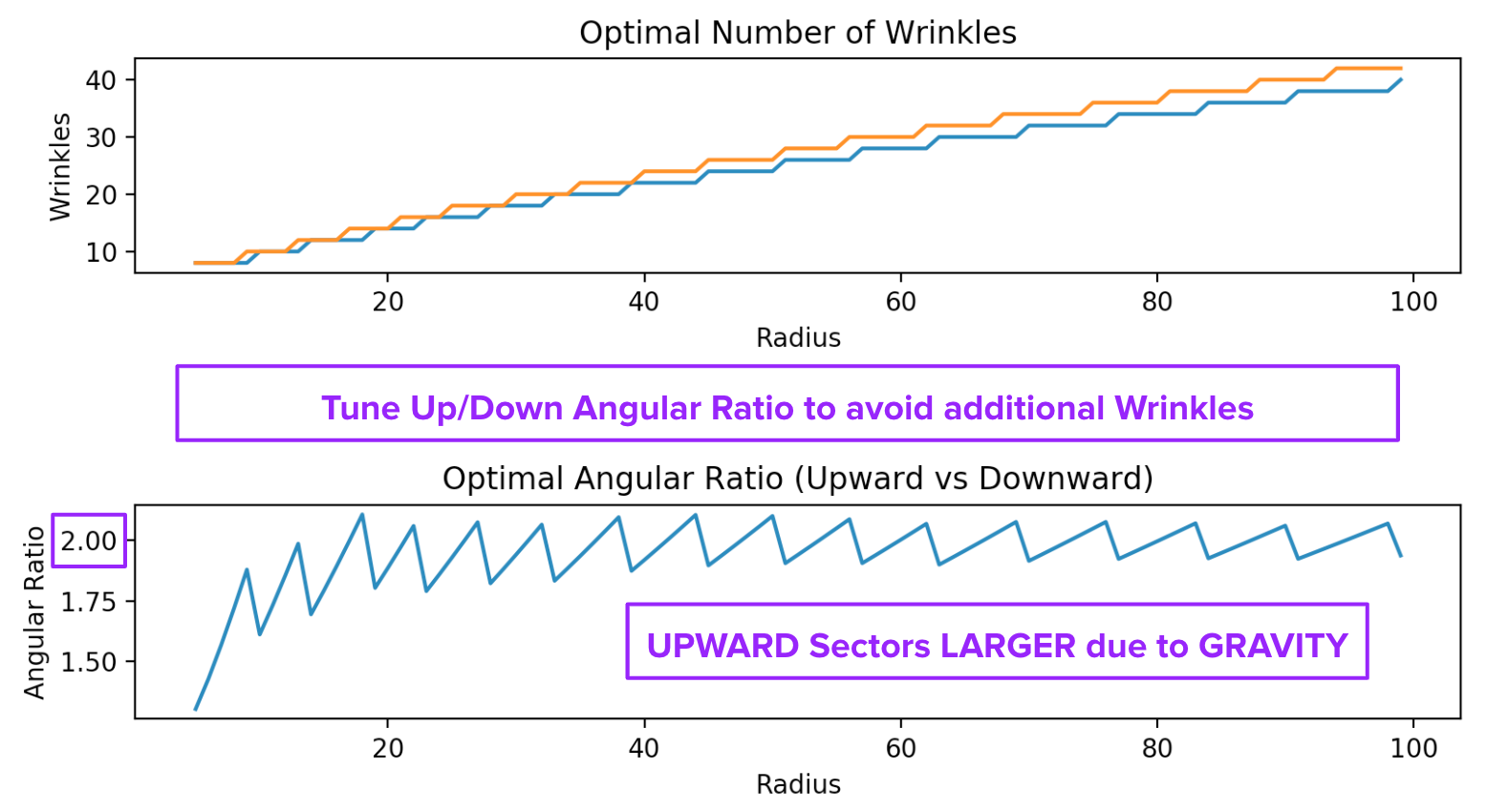
In the gravity-dominant limit , the optimal angular ratio between the upward- and downward-curving sectors for surfaces is 2:1. This is also the case with surfaces with straight asymptotic lines. This is confirmed analytically and numerically in a forthcoming paper Yamamoto2021Role.
At smooth () points, there are 4 sectors, so a “non-branch” point has degree 2. In contrast, a branch point has degree and we define the excess degree by subtracting 2 from the degree of a branch point. The excess degrees of the branch points add, so that the total number of wrinkles in the sheet, which is equal to the number of sectors that intersect the boundary, is given by
where the sum is over all the branch points on the surface and is the degree of the -th branch point. For piecewise quadratic surfaces with a single branch point at the origin, the total number of wrinkles is the same at all radial locations and equals twice the degree of the origin. The scaling of the number of wrinkles for the (restricted) minimizers with equal up-down angles, as well as independent up-down angles is shown in Fig. 16. Although the scaling of the total number of wrinkles with respect to the radius is the same, allowing for an asymmetry between the upward- and downward-curving sectors slightly delays the introduction of a new wrinkle with increasing radius of the domain. This is illustrated in the top plot in Fig. 16. The bottom plot shows that, before the creation of another wrinkle, the angular ratio between the upward- and downward-curving sectors gradually increases to approximately 2:1. It turns out that this is energetically more efficient until the radius becomes large enough that it is beneficial to create an additional wrinkle. Then, in the instant that a new wrinkle is created, the angular ratio lowers, making the upward- and downward-curving sectors more symmetric again.
Balancing the bending and gravity energies reveals a power-law relationship between the optimal number of wrinkles (corresponding to the lowest total energy) and the radius , where the optimal number of wrinkles is proportional to . Subsequently, it can also be shown that the energy scales as . The number of wrinkles with respect to the dimensionless parameter for isometries scales as . These scaling laws can be confirmed both numerically and analytically; see Fig. 17.

Given the zero-stretching constraint given by Eq.(7), we have
where and are the principal curvatures in the azimuthal and radial directions, respectively. For wrinkles, i.e., pairs of upward and downward curving sectors, we have
With this constraint and assuming a piecewise solution to the zero-stretching constraint PDE given by Eq.(7) given by odd extensions of Eq. (17) over a unit disc with a horizontal tangent plane at the origin (i.e., ), we have that the vertical height of the solution is
where is the arclength of the -projection of a single upward or downward curving sector of the solution over and is its radius. Consequently, setting to approximate the scaled dimensionless energy functional given by Eq.(16) we obtain
Therefore, assuming large , we drop the term to obtain
| (18) |
Finally, optimizing with respect to gives
| (19) |
which implies that
for fixed and . Substituting Eq.(19) into Eq.(18) and solving for , we obtain
again for fixed and .
Fig. 18 is a plot of the (scaled) energy as a function of the dimensionless parameter for (no branch point) and (with branch points) isometries. The red curve is for those isometries with straight asymptotic lines. The middle, purple curve is for general isometries where the asymptotic lines may be curved, i.e. the two (and/or ) edges incident on a vertex are not necessarily collinear. The orange and blue curves are for isometries with a single branch point at the origin and an out-of-plane displacement surface with straight asymptotic lines. While the orange curve is for isometries with upward- and downward-curving sectors restricted to be of equal angular extent, the blue curve is for surfaces that allow these sector angles to be different. The green curve is for isometries allowing for one generation of offsetted branch points, i.e. one iteration of surgery as depicted in Fig. 9.

The red and purple curves in Fig. 18 correspond, respectively, to a pure quadratic function, with no branch points and identical rhombi, and a piecewise function where all the interior vertices still have degree four, so there are no branch points, while the rhombi themselves are not necessarily congruent. Unsurprisingly, there is an energy gap between the red and purple curves to the left of the plot (Fig. 18) since the sheet can exploit the additional freedom of varying the shapes of the rhombi to further lower the center of mass thereby decreasing the gravitational potential energy with minimal increases in the bending energy.
The introduction of a single branch point at the origin of increasing degrees, further flattens the sheet by generating an increasing number of wrinkles and, thereby, lowering the gravity energy dramatically. Of course, the accompanying increase in bending energy with higher degree branch points limits how many wrinkles are generated due to a balance of bending and gravity. However, these surfaces are no longer , but rather .
The energetic difference between the orange and blue curves amounts to only a slight vertical offset with no difference in the scaling . By optimally tuning the angular ratio between the upward- and downward-curving sectors to be closer to 2:1, the surface is able to attain a lower center of mass and, hence, lower the overall energy. Offsetted branch points also allow for decreases in the energy, but numerical experiments suggest that the energy scaling remains the same Yamamoto2021Role.
3.5 Dynamics of a rolling hyperbolic sheet


The conventional formulation of elasticity models the deformation of an elastic object as a map from the Lagrangian (material) frame to the Eulerian (lab) frame . Our construction of small-slopes isometries in Section 2.1 suggests that there is a third natural frame for thin hyperbolic sheets, namely its asymptotic (skeleton) frame, . While it is adequate to use conventional formulations of elasticity, it might be profitable to consider formulations that use all three frames. We illustrate this in Fig. 19 with an example which shows a smooth saddle, that rolls without slipping. For a hyperelastic material, the deformation costs zero energy and is thus a Goldstone mode although the sheet is not rigid and undergoes an elastic bending deformation. More realistic modeling, following the approach in acharya2020continuum will yield a small amount of dissipation per rotation period. In any case, the dynamics is entirely driven by the rotation of the asymptotic frame (the red/blue lines give the ruling) with respect to the material frame (green triangle painted on the material).
Let denote the asymptotic coordinates corresponding to two families of rulings whose projections are mutually orthogonal. A solution to with these rulings is given by and . We can now solve Eq. (4) for the in-plane displacements to get
Because we will consider deformations that are expressible as the action of 2d rotations, it is useful to introduce the complex variables , for the asymptotic coordinates and , for the material coordinates on the sheet. The Eulerian description of this static deformation, which includes the in-plane displacements, is given by the mapping :
where is determined by the condition that the minimum of on the disk , which occurs at , is on the horizontal at height 0, so .
We can now compute the dynamic shape of rotating sheet, as well as its Lagrangian to Eulerian deformation map through
| (20) |
where represents the angular velocity of the “shape” in the lab frame and represents the angular velocity of the asymptotic frame with respect to the material. The rate at which the material rotates with respect to the lab is therefore . In Fig. 19, the angular velocities and are positive, i.e., the rotation is counterclockwise as viewed from above.
The trajectory of a material particle with Lagrangian coordinates is given by ; therefore, the instantaneous velocity of a material particle is
The rolling condition dictates that points of contact between the rolling body and the surface it contacts must have zero velocity. The points of contact are given by and , which correspond to the material points and . Setting the velocity at these points to 0 we get
| (21) |
Substituting this relation in Eq. (20) gives the full description of the deformation of the rotating saddle through a one parameter family of isometries including the correct imposition of the “rolling” constraint: an Eulerian condition.
4 Discussion
In this work we present a general method for constructing exact isometric immersions of hyperbolic metrics with finite bending content in the small-slope setting. We showed that the relevant singularities in free hyperbolic sheets are therefore branch points and lines of inflection. These defects are unique in that the elastic energy does not concentrate on the defects as . This is in contrast to crumpled intrinsically flat sheets in which the stretching and bending energies are equipartitioned across across elastic ridges lobkovsky and around -cones benAmar1997Crumpled. Indeed, the existence of exact small-slope isometries with finite bending content ensure that the elastic energy of global minimizers scales like which is much smaller than , the energy for crumpled intrinsically flat sheets lobkovsky; conti2008confining.
In this work, we develop ‘geometric’ methods that are directly applicable to the non-smooth configurations describing the vanishing thickness, , limit of hyperbolic sheets. For non-zero but small thickness , we expect that the lines of inflection and branch points are smoothed out on a small scale gemmer2012defects, and there is an alternative framework for deriving thermodynamically consistent models, including the effects of dissipation, in the setting acharya2020continuum.
One consequence of our construction of piecewise smooth isometries is that there are continuous families of low-energy states obtained by appropriately gluing together isometries and “floppy modes” that come from variations within these families. Thin hyperbolic sheets are therefore easily deformed by weak stresses and the pattern selected may be sensitive to the dynamics of the swelling process, experimental imperfections, or other external forces. A statistical description of the singularities and their interactions is therefore a natural approach to study this system, in contrast to a static approach that seeks to find the global energy minimum. This problem is indeed very much open; a first step might be to analyze the energy scaling, following the discussion in §3.2, of a surface with a prescribed distribution of branch points.
The examples we presented in this work are but a small sample of the nontrivial mechanical properties of hyperbolic sheets. This “extreme mechanics” can be exploited by controlling branch points, which, as we discussed above, are not tied to material points and can thus move “easily”. We conjecture these nonlinear mechanical properties are exploited by a variety of biological systems for locomotion or to effect large morphological changes with a small energy budget. These mechanical properties can therefore confer evolutionary advantages to living organisms and thus contribute to the observed ubiquity of hyperbolic forms in nature wertheim2016corals.
Finally, we believe the results presented in this work extend more generally to hyperbolic Monge-Ampere equations in various geometries, as we have outlined in this paper, but further work is needed for a precise formulation and rigorous proofs of the generalizations.
Acknowledgments
We warmly acknowledge the many insightful conversations we’ve had with Benny Davidovitch, Eran Sharon, and Ian Tobasco on these topics. We are grateful to Ido Levin who helped make the PVS gel samples and to Eran Sharon for providing the lab space and equipment for the force measurement experiments. KY and SV gratefully acknowledge the hospitality of the Racah Institute of Physics at the Hebrew University, where portions of this work were carried out. KY also acknowledges funding from the U.S.-Israel Binational Science Foundation Prof. Rahamimoff Travel Grant for the research visit in Israel. TS was partially supported by a Michael Tabor fellowship from the Graduate Interdisciplinary Program in Applied Mathematics at the University of Arizona. SV was partially supported by the Simons Foundation through awards 524875 and 560103. KY, ES and SV were partially supported by the NSF award DMR-1923922. KY was also partially supported by the 2018-19 Michael Tabor fellowship from the Graduate Interdisciplinary Program in Applied Mathematics at the University of Arizona, the 2020 Marshall Foundation Dissertation Fellowship from the Graduate College at the University of Arizona, and the NSF RTG grant DMS-184026.
Author Contributions
KY, TS, JG, and SV developed the theoretical formalism and performed the analytic calculations. KY, TS, and ES performed the numerical simulations. KY carried out the force measurement experiments and analyzed the data. All the authors discussed the results. All the authors contributed to writing the final version of the manuscript. All of the authors read and approved the final manuscript.
References
- (1) M. Wertheim, Corals, crochet and the cosmos: how hyperbolic geometry pervades the universe, theconversation.com (2016 (accessed June 21, 2020))
- (2) S. Nechaev, R. Voituriez, J. Phys. A: Mathematical and General 34, 11069 (2001)
- (3) E. Sharon, B. Roman, M. Marder, G.S. Shin, H.L. Swinney, Nature 419, 579 (2002)
- (4) E. Sharon, M. Marder, H.L. Swinney, American Scientist 92, 254 (2004)
- (5) E. Sharon, B. Roman, H.L. Swinney, Physical Review E (Statistical, Nonlinear, and Soft Matter Physics) 75, 046211 (2007)
- (6) H. Liang, L. Mahadevan, Proceedings of the National Academy of Sciences 108, 5516 (2011)
- (7) E. Sharon, M. Sahaf, in Plant Biomechanics: From Structure to Function at Multiple Scales, edited by A. Geitmann, J. Gril (Springer International Publishing, 2018), pp. 109–126
- (8) U. Nath, B.C. Crawford, R. Carpenter, E. Coen, Science 299, 1404 (2003)
- (9) B. Audoly, A. Boudaoud, Phys. Rev. Lett. 91, 086105 (2003)
- (10) E. Efrati, Y. Klein, H. Aharoni, E. Sharon, Physica D: Nonlinear Phenomena 235, 29 (2007)
- (11) Y. Klein, E. Efrati, E. Sharon, Science 315, 1116 (2007)
- (12) J. Kim, J.A. Hanna, M. Byun, C.D. Santangelo, R.C. Hayward, Science 335, 1201 (2012)
- (13) A. Goriely, M.B. Amar, Phys. Rev. Lett. 94, 198103 (2005)
- (14) M. Ben Amar, A. Goriely, J. Mech. Phys. Solids 53, 2284 (2005)
- (15) E. Efrati, E. Sharon, R. Kupferman, Journal of the Mechanics and Physics of Solids 57, 762 (2009)
- (16) E. Efrati, E. Sharon, R. Kupferman, Soft Matter 9, 8187 (2013)
- (17) P. Bella, R.V. Kohn, J. Nonlinear Sci. 24, 1147 (2014)
- (18) P. Bella, R.V. Kohn, Communications on Pure and Applied Mathematics 67, 693 (2014)
- (19) I. Tobasco, Archive for Rational Mechanics and Analysis 239, 1211 (2021)
- (20) I. Tobasco, Y. Timounay, D. Todorova, G.C. Leggat, J.D. Paulsen, E. Katifori, Exact solutions for the wrinkle patterns of confined elastic shells (2020), 2004.02839
- (21) Q. Han, J.X. Hong, Isometric Embedding of Riemannian manifolds in Euclidean spaces, Vol. 130 (American Mathematical Society Providence, RI, 2006)
- (22) J. Gemmer, E. Sharon, T. Shearman, S.C. Venkataramani, Europhys. Lett. 114, 24003 (2016)
- (23) J.J. Stoker, Differential geometry (John Wiley & Sons Inc., 1989), reprint of the 1969 original, A Wiley-Interscience Publication
- (24) S.C. Venkataramani, T.A. Witten, E.M. Kramer, R.P. Geroch, J. Math. Phys. 41, 5107 (2000)
- (25) A. Lobkovsky, S. Gentges, H. Li, D. Morse, T.A. Witten, Science 270, 1482 (1995)
- (26) M. Ben Amar, Y. Pomeau, Proceedings of the Royal Society of London. Series A: Mathematical, Physical and Engineering Sciences 453, 729 (1997)
- (27) T. Witten, Reviews of Modern Physics 79, 643 (2007)
- (28) A.E. Lobkovsky, Phys. Rev. E 53, 3750 (1996)
- (29) S. Conti, F. Maggi, Arch. Ration. Mech. Anal. 187, 1 (2008)
- (30) B. Davidovitch, Y. Sun, G.M. Grason, Proceedings of the National Academy of Sciences 116, 1483 (2019)
- (31) Y.C. Fung, Foundations of solid mechanics (Prentice-Hall, Englewood Cliffs, N.J., 1965), ISBN 0133299120 9780133299120
- (32) M. Lewicka, L. Mahadevan, M.R. Pakzad, Proc. Roy. Soc. London Ser. A 467, 402 (2011)
- (33) M. Lewicka, M. Reza Pakzad, ESAIM: Control, Optimisation and Calculus of Variations 17, 1158 (2011)
- (34) H. Aharoni, D.V. Todorova, O. Albarrán, L. Goehring, R.D. Kamien, E. Katifori, Nature Communications 8, 15809 (2017)
- (35) O. Albarrán, D.V. Todorova, E. Katifori, L. Goehring, Curvature controlled pattern formation in floating shells (2018), 1806.03718
- (36) J. Hure, B. Roman, J. Bico, Phys. Rev. Lett. 109, 054302 (2012)
- (37) H. King, R.D. Schroll, B. Davidovitch, N. Menon, Proceedings of the National Academy of Sciences 109, 9716 (2012)
- (38) T.L. Shearman, S.C. Venkataramani, Journal of Nonlinear Science 31, 13 (2021)
- (39) N.S. Trudinger, X.J. Wang, in Handbook of geometric analysis. No. 1 (Int. Press, Somerville, MA, 2008), Vol. 7 of Adv. Lect. Math. (ALM), pp. 467–524
- (40) G. De Philippis, A. Figalli, Bull. Amer. Math. Soc. (N.S.) 51, 527 (2014)
- (41) L. Caffarelli, J.J. Kohn, L. Nirenberg, J. Spruck, Commun. Pure Appl. Math. 38, 209 (1985)
- (42) J.D. Benamou, B.D. Froese, A.M. Oberman, ESAIM: Mathematical Modelling and Numerical Analysis - Modélisation Mathématique et Analyse Numérique 44, 737 (2010)
- (43) A.I. Bobenko, J.M. Sullivan, P. Schröder, G.M. Ziegler, Discrete differential geometry (Springer, 2008)
- (44) E. Huhnen-Venedey, T. Rörig, Geometriae Dedicata 168, 265 (2014)
- (45) A. Hatcher, Algebraic topology (Cambridge University Press, Cambridge, 2002)
- (46) R. Sauer, Mathematische Zeitschrift 52, 611 (1950)
- (47) W. Wunderlich, Österreich. Akad. Wiss. Math.-Nat. Kl. S.-B. IIa. 160, 39 (1951)
- (48) S. Kim, C. Laschi, B. Trimmer, Trends in biotechnology 31, 287 (2013)
- (49) M.H. Amsler, Mathematische Annalen 130, 234 (1955)
- (50) J.A. Gemmer, S.C. Venkataramani, Physica D: Nonlinear Phenomena 240, 1536 (2011)
- (51) M. Pezzulla, S.A. Shillig, P. Nardinocchi, D.P. Holmes, Soft Matter 11, 5812 (2015)
- (52) K.K. Yamamoto, S.C. Venkataramani, Weak forces and the morphology of hyperbolic elastic plates. (2021), in preparation.
- (53) A. Acharya, S.C. Venkataramani, Materials Theory 4, 2 (2020)
- (54) J. Gemmer, S. Venkataramani, Nonlinearity 25, 3553 (2012)