跳到论文正文
W Papers独立论文阅读器 arXiv:2103.10353 论文正文 计算阅读时间 · 0%
引用这篇论文根据当前论文元数据生成,正式投稿前建议核对。


License: CC BY 4.0
arXiv:2103.10353v1 [math.DG] 18 Mar 2021

Swallowtails and cone-like singularities on a maxface

Pradip Kumar Address: Department of Mathematics, Shiv Nadar University, Dadri 201314, Uttarpradesh, India. Email address: pradip.kumar@snu.edu.in and Anu Dhochak Address: Department of Mathematics, Shiv Nadar University, Dadri 201314, Uttarpradesh, India. Email address: ad404@snu.edu.in
Abstract.

When a connected component of the set of singular points of the maxface XX consists of only generalized cone-like singular point, we construct a sequence of maxfaces XnX_{n}, with an increasing number of swallowtails, converging to the maxface XX. We include the general discussion toward this.

Key words and phrases: 
maxface singularities, swallowtails, cone-like
2020 Mathematics Subject Classification
53A35

1. Introduction

Maximal surfaces in the Lorentz-Minkowski space 𝔼13\mathbb{E}_{1}^{3} are space-like immersions that maximize area locally. They are similar to the minimal surfaces in ℝ3\mathbb{R}^{3}, as both are zero mean curvature surface and can be constructed using many similar methods but in the maximal surfaces non-isolated singularities appear.

Estudillo and Romero [2] named generalized maximal immersion for the maximal surfaces with singularities. They are of two types, branched and non branched. Non-branched maximal immersions are the one when limiting tangent plane contains a light-like vector. The Maxface, introduced by Umehara and Yamada [12], are non branched generalized maximal immersions.

Umehara and Yamada [12] have shown that all the maxface, as a map to ℝ3\mathbb{R}^{3}, become frontal, and a few of them near the singularity become front. As a front and frontal, in [4], [5], [6], [12], [11], we see authors have discussed various singularities: swallowtails, cuspidal-edge, cuspidal cross cap, cuspidal butterflies, cuspidal S1−S_{1}^{-}. There is another important singularity, called the cone-like singularity. Cone-like singularities, introduced by O. Kobayashi [10], are non isolated and discussed in [3], [5] etc.

In [7], Kim and Yang gave an example of family of maxfaces for each natural number nn, that has swallowtails in an increasing order. We call it (a name given by the authors in [5]) Kim and Yang’s toroidal maxface. The authors discussed the global properties of this toroidal maxface. The family of toroidal maxfaces seems to “converge" to the cone-like. Moreover, in [5], the authors talked about trinoids with swallowtails whose computer graphics look cone-like. All these poses a question, if we start from a maxface having a cone-like singularity (or generalized cone-like) then, can we find a sequence of maxfaces having an increasing number of swallowtails, and converging to the former one?

In this article, we discuss the general situation, we start from a maxface with generalized cone-like singularity, and we construct the sequence in various cases. Let λ\lambda be a non-constant real analytic curve, whose trace is compact, when λ\lambda satisfies certain conditions, in section 4, we prove the following theorem.

Theorem (Theorem: 4.4).

Let XX be a maxface having generalized cone-like singularity on t​r​a​c​etrace of λ\lambda, with singular Björling data {λ,α,β}\{\lambda,\alpha,\beta\}. Moreover the data {λ,α,β}\{\lambda,\alpha,\beta\} has a sequence of the scaling functions as in the definition 4.1. Then there is a sequence of maxfaces XnX_{n} defined on a neighborhood Ω\Omega of trace of λ\lambda, having an increasing number of swallowtails, and sequence of maxfaces converges (in the norm ∥.∥Ω\|\;.\;\|_{\Omega}) to XX, having cone-like.

A significant class of maxface (defined locally) can be constructed using the singular Björling problem introduced by Kim and Yang in [8] and also discussed in [1]. Given a null curve γ\gamma and a null vector field on the real axis or the unit circle, in [1], [8], authors have constructed the maxface. In section 3, we start with the singular Björling problem when we expect singularities lie on the trace of a non-constant smooth curve λ\lambda. Further in section 3, we give necessary and sufficient conditions (in propositions: 3.1, 3.2) on the singular Björling data (defined on the trace of λ\lambda) such that singularity is of swallowtail or generalized cone-like.

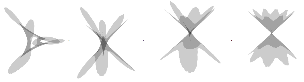
In section 4, we prove theorem 4.4 and an example of a sequence of maxfaces having an increasing number of swallowtails converging to the Lorentzian Catenoid. All the discussion is local that is near a singular curve.
Refer to caption
Figure 1. Maxfaces converging to the Lorentzian Catenoid

2. Preliminaries

The Lorentz-Minkowski space 𝔼13\mathbb{E}_{1}^{3} is a vector space ℝ3\mathbb{R}^{3} with metric ⟨,⟩:ℝ3×ℝ3→ℝ\langle\;,\;\rangle:\mathbb{R}^{3}\times\mathbb{R}^{3}\to\mathbb{R} defined by ⟨(a1,b1,c1),(a2,b2,c2)⟩:=a1​a2+b1​b2−c1​c2,\langle(a_{1},b_{1},c_{1}),(a_{2},b_{2},c_{2})\rangle:=a_{1}a_{2}+b_{1}b_{2}-c_{1}c_{2}, where (a1,b1,c1)(a_{1},b_{1},c_{1}) and (a2,b2,c2)(a_{2},b_{2},c_{2}) are two vectors in ℝ3.\mathbb{R}^{3}. In the following, we write the Weierstrass-Enneper representation of the maxface given by Umehara and Yamada [12].

2.1. Weierstrass Enneper representation

Let MM be a Riemann surface, the map X:M→𝔼13X:M\to\mathbb{E}_{1}^{3} be a maxface if and only if there is a pair (g,f)(g,f) of meromorphic function and a holomorphic 1-form on MM such that (1+|g|2)2​|f|2(1+|g|^{2})^{2}|f|^{2} gives a positive definite Riemannian metric on MM, and |g||g| is not identically equal 11. Moreover for the map Φ:=((12​(1+g2),i2​(1−g)2,−g)​f)\Phi:=\left((\frac{1}{2}(1+g^{2}),\frac{i}{2}(1-g)^{2},-g)f\right), Re∫γjΦ=0,(j=1,..,N)Re\int_{\gamma_{j}}\Phi=0,\;\;\;\;(j=1,..,N) for loops {γj}j=1N\{\gamma_{j}\}_{j=1}^{N} such that [γj][\gamma_{j}] are generators of π1​(M)\pi_{1}(M) and X⁡(p)=R​e​∫opΦX(p)=Re\int_{o}^{p}\Phi.

2.2. Singularities

Various singularities appear on the maxface. Here we review a few of these. We start by recalling the definition of 𝒜−\mathcal{A}- equivalence as in [6], [12].

Two smooth maps X:Ω⊂ℝ2→𝔼13X:\Omega\subset\mathbb{R}^{2}\to\mathbb{E}_{1}^{3} and Y:𝒱⊂ℝ2→𝔼13Y:\mathcal{V}\subset\mathbb{R}^{2}\to\mathbb{E}_{1}^{3} are said to be 𝒜−\mathcal{A}-equivalent at the points p∈Ωp\in\Omega and q∈𝒱q\in\mathcal{V} if there exists a local diffeomorphism η\eta of ℝ2\mathbb{R}^{2} with η⁡(p)=q\eta(p)=q and a local diffeomorphism Φ\Phi of 𝔼13\mathbb{E}_{1}^{3} with Φ⁡(X⁡(p))=Y⁡(q)\Phi(X(p))=Y(q) such that Y=Φ∘X∘η−1Y=\Phi\circ X\circ\eta^{-1}.

Definition 2.1 (Swallowtails [6], [12]).

A maxface X:Ω⊂ℂ→𝔼13X:\Omega\subset\mathbb{C}\to\mathbb{E}_{1}^{3} is said to have a swallowtail at p∈Ωp\in\Omega if at p∈Ωp\in\Omega and (0,0)∈ℝ2(0,0)\in\mathbb{R}^{2}, XX is 𝒜\mathcal{A}-equivalent to fs​w​(u,v)=(3​u4+u2​v, 4​u3+2​u​v,v);(u,v)∈ℝ2f_{sw}(u,v)=(3u^{4}+u^{2}v,\,4u^{3}+2uv,\,v)\,;\,(u,v)\in\mathbb{R}^{2}.

Definition 2.2 (Shrinking singularity [8]).

For a maxface X:Ω→𝔼13X:\Omega\to\mathbb{E}_{1}^{3}, we call p∈Ωp\in\Omega a shrinking singular point if there is some Up⊂ΩU_{p}\subset\Omega and a regular embedded curve γ:I⊂Up→Ω\gamma:I\subset U_{p}\to\Omega, such that every point of γ⁡[I]\gamma[I] singularity and X∘γX\circ\gamma is a single point.

Definition 2.3 (Generalized cone-like singularity and cone-like singularity [5]).

Let ∑0\sum_{0} be the connected component of the set of all admissible singular points on a generalized maximal immersion X:Ω→𝔼13X:\Omega\to\mathbb{E}_{1}^{3}. Each point of ∑0\sum_{0} is called a generalized cone-like singular point if ∑0\sum_{0} is compact and the image X(∑0)X(\sum_{0}) is a single point. Moreover, if there is a neighborhood UU of ∑0\sum_{0} such that X(U∖∑0)X(U\setminus\sum_{0}) is embedded, then each point of ∑0\sum_{0} is called a cone-like singular point.

If the trace of λ\lambda is compact and it is a connected component of the singularity, then the shrinking singularity becomes generalized cone-like. For examples and detailed discussion, we refer to [6], [8], [12] etc.

For a maxface X:Ω→𝔼13X:\Omega\to\mathbb{E}_{1}^{3} with the Weierstrass data {g,f}\{g,f\}, the authors in [5], [8], [12] have given a very useful criterion to check the nature of singularity at a particular point. For a maxface, if pp is a singularity, then there exists a curve λ\lambda on a neighborhood of pp such that every point on the trace of λ\lambda is a singularity. The curve λ\lambda is said to be a singular curve and the vector η\eta along λ\lambda is said to null curve if d​Xλ⁡(t)​(η)=0dX_{\lambda(t)}(\eta)=0. Umehara and Yamada [12] have shown that in a maxface, such direction is uniquely determined and calculated in terms of Weierstrass data.

Following [12], in terms of the Weierstrass data {g,f}\{g,f\}, and in terms of η\eta, λ\lambda, we recall the functions:

Definition 2.4 ([12]).

On a neighborhood UpU_{p} of a singularity pp, we define A⁡(z):=g′g2​fA(z):=\frac{g^{\prime}}{g^{2}f}.

Since λ\lambda is a singular curve parameterized on II, we define H⁡(t)=D​e​t​(λ′​(t),η⁡(t))H(t)=Det(\lambda^{\prime}(t),\eta(t)) for all t∈It\in I.

Moreover[12] a maxface becomes front on a neighborhood of singularity if R​e​(A⁡(λ⁡(t))≠0CLOSERe(A(\lambda(t))\neq 0 at the singular points and as a front, singularity at p=λ⁡(t)p=\lambda(t) is swallowtail if and only if H′​(t)≠0H^{\prime}(t)\neq 0.

3. Singular Björling problem and the necessary and sufficient conditions for few singularities

In this section, we will discuss the singular Björling problem in a general case when we expect the singularities to lie on the trace of a smooth non-constant curve. It is similar to the discussion in [1], [8]. Further, we will find the necessary and sufficient conditions on the singular Björling data so that singularities are of generalized cone-like or swallowtails.

3.1. Singular Björling problem on a curve

We start by defining the singular Björing data similar to the way Kim and Yang have given in [8].

Definition 3.1 (Singular Björling data).

This is a triplet {λ,α,β}\{\lambda,\alpha,\beta\}, where

  1. (1)

    λ:I→ℂ\lambda:I\to\mathbb{C} be a smooth curve such that for all t∈It\in I, λ′​(t)≠0\lambda^{\prime}(t)\neq 0.

  2. (2)

    α\alpha be a null curve and β\beta be a null vector field defined on II and for all t∈It\in I, ⟨α′​(t),β⁡(t)⟩=0\langle\alpha^{\prime}(t),\beta(t)\rangle=0. Moreover, either α′​(t)≠0\alpha^{\prime}(t)\neq 0 or β⁡(t)≠0\beta(t)\neq 0 for all t∈It\in I.

  3. (3)

    The map given by ϕ⁡(λ⁡(t))=α′​(t)−i​β​(t)\phi(\lambda(t))=\alpha^{\prime}(t)-i\beta(t) has an extension ϕ⁡(z)\phi(z) on the trace of λ\lambda.

  4. (4)

    Analytic extension g⁡(w)g(w) of g⁡(λ⁡(t))=G⁡(t)g(\lambda(t))=G(t) where

    (3.1) G⁡(t):={α1′​(t)+i​α2′​(t)α3′​(t)​ if ​α′​(t)≠0β1​(t)+i​β2​(t)β3​(t)​ if ​β3​(t)≠0G(t):=\begin{cases}\frac{\alpha_{1}^{\prime}(t)+i\alpha_{2}^{\prime}(t)}{\alpha_{3}^{\prime}(t)}\;\text{ if }\alpha^{\prime}(t)\neq 0\\ \frac{\beta_{1}(t)+i\beta_{2}(t)}{\beta_{3}(t)}\text{ if }\beta_{3}(t)\neq 0\end{cases}

    and |g⁡(w)||g(w)| is not identically equal to 1.

For the data {λ,α,β}\{\lambda,\alpha,\beta\}, if R​e​∫γjϕ⁡(z)​𝑑zRe\int_{\gamma_{j}}\phi(z)dz vanishes for all loops γj\gamma_{j} on a neighborhood Ω\Omega of trace of λ\lambda. Then the map X:=(X1,X2,X3):Ω→𝔼13X:=(X_{1},X_{2},X_{3}):\Omega\to\mathbb{E}_{1}^{3}, given by

(3.2) Xλ,α,β​(z)=R​e​(∫λ⁡(t0)zϕ⁡(w)​𝑑w)X_{\lambda,\alpha,\beta}(z)=Re\left(\int_{\lambda(t_{0})}^{z}\phi(w)dw\right)

is well defined and it gives a generalized maximal immersions on Ω\Omega, containing the trace of λ\lambda. Moreover the trace of λ\lambda is a subset of the singular set. The generalized maximal immersion given in the equation 3.2 is unique up to translations (we have many choices of λ⁡(t0)\lambda(t_{0})).

Example 3.2.

Let λ⁡(t)=(t,0)\lambda(t)=(t,0), and α\alpha and β\beta be real analytic curve and vector field respectively. Then ϕ⁡(z)=α′​(z)−β⁡(z)\phi(z)=\alpha^{\prime}(z)-\beta(z) is analytic and it gives a generalized maximal immersion. This is the case of the singular Björling problem as introduced and discussed by Kim and Yang in [8].

Example 3.3.

Let λ⁡(t)=ei​t\lambda(t)=e^{it}, 0≤t≤2​π0\leq t\leq 2\pi. Let α′​(t)=(cos⁡(t),sin⁡(t),1)\alpha^{\prime}(t)=(\cos(t),\sin(t),1) and β⁡(t)=(0,0,0)\beta(t)=(0,0,0), then

ϕ⁡(ei​t)\displaystyle\phi(e^{it}) =(cos⁡(t),sin⁡(t),1)\displaystyle=(\cos(t),\sin(t),1)
=(ei​t+e−i​t2,ei​t−e−i​t2​i,1)\displaystyle=\left(\dfrac{e^{it}+e^{-it}}{2},\dfrac{e^{it}-e^{-it}}{2i},1\right)

it has analytic extension ϕ⁡(z)=(z2+12​z,i⁡(12​z−z2),1)\phi(z)=(\frac{z}{2}+\frac{1}{2z},i(\frac{1}{2z}-\frac{z}{2}),1) in a annular region containing unit circle. It gives a generalized maximal immersion in an annular region that contains the unit circle.

The generalized maximal immersion as in the equation 3.2 is a maxface on a neighborhood of trace of λ\lambda. Moreover, for z=λ⁡(t)z=\lambda(t), f⁡(z)=ϕ1​(z)−i​ϕ2​(z)=(α1′​(t)+β2​(t))−i⁡(α2′​(t)+β1​(t))f(z)=\phi_{1}(z)-i\phi_{2}(z)=(\alpha_{1}^{\prime}(t)+\beta_{2}(t))-i(\alpha_{2}^{\prime}(t)+\beta_{1}(t)). Therefore ff is never zero on Trace of λ\lambda.

The Gauss map is given by

g⁡(z)=−ϕ3​(z)ϕ1​(z)−i​ϕ2​(z)=−ϕ1​(z)+i​ϕ2​(z)ϕ3​(z),g(z)=-\frac{\phi_{3}(z)}{\phi_{1}(z)-i\phi_{2}(z)}=-\frac{\phi_{1}(z)+i\phi_{2}(z)}{\phi_{3}(z)},

and g⁡(λ⁡(t))=G⁡(t)g(\lambda(t))=G(t), as in the equation 3.1.

3.2. Null direction

Let Xλ,α,β:Ω→𝔼13X_{\lambda,\alpha,\beta}:\Omega\to\mathbb{E}_{1}^{3} be the maxface for a fixed t0t_{0} as in the equation 3.2. Since d​X=12​Xz​d​z+12​Xz¯​d​z¯=ϕ⁡(z)​d​z+ϕ⁡(z)¯​d​z¯dX=\frac{1}{2}X_{z}dz+\frac{1}{2}X_{\overline{z}}d\overline{z}=\phi(z)dz+\overline{\phi(z)}d\overline{z}. At z=λ⁡(t)z=\lambda(t), we have

d​Xλ⁡(t)=(α′​(t)−i​β​(t))​d​zλ⁡(t)+(α′​(t)+i​β​(t))​d​z¯λ⁡(t)dX_{\lambda(t)}=(\alpha^{\prime}(t)-i\beta(t))dz_{\lambda(t)}+(\alpha^{\prime}(t)+i\beta(t))d\bar{z}_{\lambda(t)}

So let v=η​∂∂z¯+η¯​∂∂z¯v=\eta\frac{\partial}{\partial\bar{z}}+\bar{\eta}\frac{\partial}{\partial\bar{z}} such that d​Xλ⁡(t)​(v)=0dX_{\lambda(t)}(v)=0, we have (α3′​(t)−i​β3​(t))​η+(α3′​(t)+i​β3​(t))​η¯=0(\alpha_{3}^{\prime}(t)-i\beta_{3}(t))\eta+(\alpha_{3}^{\prime}(t)+i\beta_{3}(t))\overline{\eta}=0, that is:

α3′​(t).R​e​(η)+β3​(t)​I​m​(η)=0.\alpha_{3}^{\prime}(t).Re(\eta)+\beta_{3}(t)Im(\eta)=0.

Therefore the null direction at each λ⁡(t)\lambda(t) is given by

(3.3) η⁡(t)=−β3​(t)+i​α3′​(t).\eta(t)={-\beta_{3}(t)+i\alpha_{3}^{\prime}(t)}.

3.3. Calculation for A⁡(t)A(t) and H′​(t)H^{\prime}(t)

In the following, we will calculate A⁡(λ⁡(t))A(\lambda(t)) and H′​(t)H^{\prime}(t) as given in the equation 2.4. We write it here again

A⁡(λ⁡(t))=G′​(t)G2​(t)​λ′​(t)​f​(λ⁡(t)CLOSE, and ​H​(t)=D​e​t​(λ′​(t),η⁡(t)).A(\lambda(t))=\frac{G^{\prime}(t)}{G^{2}(t)\lambda^{\prime}(t)f(\lambda(t)},\text{ and }H(t)=Det(\lambda^{\prime}(t),\eta(t)).

We define

(3.4) D⁡(β12,β12′):=β1​β2′−β2​β1′,D⁡(α12′,α12′′):=α1′​α2′′−α2′​α1′′.D(\beta_{12},\beta_{12}^{\prime}):=\beta_{1}\beta_{2}^{\prime}-\beta_{2}\beta_{1}^{\prime},\;\;D(\alpha_{12}^{\prime},\alpha_{12}^{\prime\prime}):=\alpha_{1}^{\prime}\alpha_{2}^{\prime\prime}-\alpha_{2}^{\prime}\alpha_{1}^{\prime\prime}.

We have g′​(λ⁡(t)=G′​(t)λ′​(t)CLOSEg^{\prime}(\lambda(t)=\frac{G^{\prime}(t)}{\lambda^{\prime}(t)}, where GG is given by the equation 3.1.

For the case when β3​(t)≠0\beta_{3}(t)\neq 0, a straight calculation gives,

G′​(t)G2​(t).f⁡(λ⁡(t))=−D⁡(β12,β12′)(α3′2+β32)​β3+i​α3′​D​(β12,β12′)(α3′2+β32)​β32.\frac{G^{\prime}(t)}{G^{2}(t).f(\lambda(t))}=\frac{-D(\beta_{12},\beta_{12}^{\prime})}{(\alpha_{3}^{\prime 2}+\beta_{3}^{2})\beta_{3}}+i\frac{\alpha_{3}^{\prime}D(\beta_{12},\beta_{12}^{\prime})}{(\alpha_{3}^{\prime 2}+\beta_{3}^{2})\beta_{3}^{2}}.

Therefore we

A⁡(λ⁡(t))\displaystyle A(\lambda(t)) =(g′​(λ​(t)CLOSEg2​(λ⁡(t)​f​(λ⁡(t))CLOSE)=G′​(t)G2​(t).f⁡(λ⁡(t)).λ1′​(t)−i​λ2′​(t)λ1′2​(t)+λ2′2​(t)\displaystyle=\left(\frac{g^{\prime}(\lambda(t)}{g^{2}(\lambda(t)f(\lambda(t))}\right)=\frac{G^{\prime}(t)}{G^{2}(t).f(\lambda(t))}.\frac{\lambda_{1}^{\prime}(t)-i\lambda_{2}^{\prime}(t)}{\lambda_{1}^{\prime 2}(t)+\lambda_{2}^{\prime 2}(t)}
=D⁡(β12,β12′)(α3′2+β32)​β32.(λ1′2​(t)+λ2′2​(t)).(−β3+i​α3′).(λ1′​(t)−i​λ2′​(t))\displaystyle=\frac{D(\beta_{12},\beta_{12}^{\prime})}{(\alpha_{3}^{\prime 2}+\beta_{3}^{2})\beta_{3}^{2}.(\lambda_{1}^{\prime 2}(t)+\lambda_{2}^{\prime 2}(t))}.(-\beta_{3}+i\alpha_{3}^{\prime}).(\lambda_{1}^{\prime}(t)-i\lambda_{2}^{\prime}(t))
=D⁡(β12,β12′)(α3′2+β32)​β32.(λ1′2+λ2′2)((−β3λ1′+α3′λ2′)+i.(α3′λ1′+β3λ2′))\displaystyle=\frac{D(\beta_{12},\beta_{12}^{\prime})}{(\alpha_{3}^{\prime 2}+\beta_{3}^{2})\beta_{3}^{2}.(\lambda_{1}^{\prime 2}+\lambda_{2}^{\prime 2})}\left((-\beta_{3}\lambda_{1}^{\prime}+\alpha_{3}^{\prime}\lambda_{2}^{\prime})+i.(\alpha_{3}^{\prime}\lambda_{1}^{\prime}+\beta_{3}\lambda_{2}^{\prime})\right)

Similarly, we can calculate for the case when α3′​(t)≠0\alpha_{3}^{\prime}(t)\neq 0 and we get the following.

(3.5) A⁡(λ⁡(t)):={D⁡(α12′,α12′′)(λ1′2+λ2′2)​(α3′2+β32)​α3′2((−β3λ1′+α3′λ2′)+i.(α3′λ1′+β3λ2′)) if α′3(t)≠0D⁡(β12,β12′)(α3′2+β32)​β32.(λ1′2+λ2′2)((−β3λ1′+α3′λ2′)+i.(α3′λ1′+β3λ2′)) if β3(t)≠0.A(\lambda(t)):=\begin{cases}\frac{D(\alpha_{12}^{\prime},\alpha_{12}^{\prime\prime})}{(\lambda_{1}^{\prime 2}+\lambda_{2}^{\prime 2})(\alpha_{3}^{\prime 2}+\beta_{3}^{2})\alpha_{3}^{\prime 2}}\left((-\beta_{3}\lambda_{1}^{\prime}+\alpha_{3}^{\prime}\lambda_{2}^{\prime})+i.(\alpha_{3}^{\prime}\lambda_{1}^{\prime}+\beta_{3}\lambda_{2}^{\prime})\right)\;\text{ if }\alpha^{\prime}_{3}(t)\neq 0\\ \frac{D(\beta_{12},\beta_{12}^{\prime})}{(\alpha_{3}^{\prime 2}+\beta_{3}^{2})\beta_{3}^{2}.(\lambda_{1}^{\prime 2}+\lambda_{2}^{\prime 2})}\left((-\beta_{3}\lambda_{1}^{\prime}+\alpha_{3}^{\prime}\lambda_{2}^{\prime})+i.(\alpha_{3}^{\prime}\lambda_{1}^{\prime}+\beta_{3}\lambda_{2}^{\prime})\right)\text{ if }\beta_{3}(t)\neq 0.\end{cases}

Now we calculate the function H⁡(t)H(t). The null direction is given by the equation 3.3. We get H⁡(t)=λ1′​α3′+λ2′​β3H(t)=\lambda_{1}^{\prime}\alpha_{3}^{\prime}+\lambda_{2}^{\prime}\beta_{3} and therefore we have

(3.6) H′​(t)=λ1′′​α3′+λ1′​α3′′+λ2′​β3′+λ2′′​β3H^{\prime}(t)=\lambda_{1}^{\prime\prime}\alpha_{3}^{\prime}+\lambda_{1}^{\prime}\alpha_{3}^{\prime\prime}+\lambda_{2}^{\prime}\beta_{3}^{\prime}+\lambda_{2}^{\prime\prime}\beta_{3}

3.4. For shrinking and generalized cone-like

The maxface Xλ,α,βX_{\lambda,\alpha,\beta} as in the equation 3.2 has shrinking singularity on the trace of λ\lambda if and only if Xλ,α,β​(λ​(t))X_{\lambda,\alpha,\beta}(\lambda(t)) is constant and g′​(λ​(t))≠0\;\;g^{\prime}(\lambda(t))\neq 0\;\ for all t∈It\in I, where gg is the Gauss map.

This implies ∀t∈I\forall t\in I, D​Xλ⁡(t)​(λ′​(t))=0DX_{\lambda(t)}(\lambda^{\prime}(t))=0 if and only if ∀t∈I,α′​(t)​λ1′​(t)+β⁡(t)​λ2′​(t)=0\forall t\in I,\;\alpha^{\prime}(t)\lambda_{1}^{\prime}(t)+\beta(t)\lambda_{2}^{\prime}(t)=0 if and only if for all t∈I,I​m​(A⁡(t)=0CLOSEt\in I,Im(A(t)=0.

As g′​(λ⁡(t))=G′​(t)λ′​(t)≠0g^{\prime}(\lambda(t))=\dfrac{G^{\prime}(t)}{\lambda^{\prime}(t)}\neq 0 and I​m​(A⁡(t))=0Im(A(t))=0, if and only if ∀t∈I,R​e​(A⁡(t))≠0\forall t\in I,Re(A(t))\neq 0.

From above we get, ∀t∈I\forall t\in I, −β3​λ1′+α3′​λ2′≠0-\beta_{3}\lambda^{\prime}_{1}+\alpha_{3}^{\prime}\lambda_{2}^{\prime}\neq 0. Therefore R​e​(A⁡(t))≠0Re(A(t))\neq 0 if and only if D⁡(β1,β2′)≠0D(\beta_{1},\beta_{2}^{\prime})\neq 0 when β3≠0\beta_{3}\neq 0, and D⁡(α12′,α12′′)≠0D(\alpha_{12}^{\prime},\alpha_{12}^{\prime\prime})\neq 0 when α3′​(t)≠0\alpha_{3}^{\prime}(t)\neq 0.

Summarising everything here, we get the following.

Proposition 3.1.

The solution of Björling problem (as in the equation 3.2) on a neighborhood of the trace of λ\lambda, consists of only shrinking singularities on the trace of λ\lambda if and only if

  1. (1)

    ∀t∈I,α3′​(t)​λ1′​(t)+β3​(t)​λ2′​(t)=0\forall t\in I,\alpha^{\prime}_{3}(t)\lambda_{1}^{\prime}(t)+\beta_{3}(t)\lambda_{2}^{\prime}(t)=0

  2. (2)

    D⁡(β1,β2′)≠0D(\beta_{1},\beta_{2}^{\prime})\neq 0 when β3​(t)≠0\beta_{3}(t)\neq 0, and D⁡(α12′,α12′′)≠0D(\alpha_{12}^{\prime},\alpha_{12}^{\prime\prime})\neq 0 when α3′​(t)≠0\alpha_{3}^{\prime}(t)\neq 0. Here D(.,.)D(.\;,\;.) as in the equation 3.4.

In particular, if the trace of λ\lambda is compact, then the trace of λ\lambda consists of only generalized cone-like singularities.

Example 3.4.

When λ⁡(t)=ei​t\lambda(t)=e^{it}, 0≤t<2​π0\leq t<2\pi, Let α′​(t)=cos⁡t⁡(cos⁡t,sin⁡t,−1)\alpha^{\prime}(t)=\cos t(\cos t,\sin t,-1), and β⁡(t)=sin⁡t⁡(cos⁡t,sin⁡t,−1)\beta(t)=\sin t(\cos t,\sin t,-1). For this singular Björling data, the maxface as in the equation 3.2, satisfies conditions of the proposition 3.1. Moreover the trace of λ\lambda is unit circle. Therefore every point of the unit circle is a generalized cone-like singularity (in fact it is cone-like singularity).

The Weierstrass data {g,w}\{g,w\} for this maxface is {g⁡(z)=z,w⁡(z)=1z2}\{g(z)=z,w(z)=\frac{1}{z^{2}}\}. This is the Lorentzian Catenoid [9].

Example 3.5.

Let λ⁡(t)=(t,0),a<t<b\lambda(t)=(t,0),a<t<b, and α⁡(t)\alpha(t) be a constant curve. Let β\beta be a real null analytic vector field defined on II such that ∀t\forall t,(β1′​β2−β2​β1′)≠0(\beta_{1}^{\prime}\beta_{2}-\beta_{2}\beta_{1}^{\prime})\neq 0 then solution as in equation 3.2 gives shrinking singularity.

In particular, if β⁡(t)=(1−t2,2​t,1+t2)\beta(t)=(1-t^{2},2t,1+t^{2}) then we see that for all t∈ℝt\in\mathbb{R}, (β1​β2′−β2​β1′)≠0(\beta_{1}\beta_{2}^{\prime}-\beta_{2}\beta_{1}^{\prime})\neq 0. Therefore, this β\beta with any constant α\alpha gives a maxface.

Moreover, the Weierstrass data for this maxface (equation 3.2) is

{g⁡(z)=−1−z2+2​i​z1+z2,w⁡(z)=−2​z−i⁡(1−z2)}\left\{g(z)=-\frac{1-z^{2}+2iz}{1+z^{2}},w(z)=-2z-i(1-z^{2})\right\}

To treat separately the case, when λ⁡(t)=(t,0)\lambda(t)=(t,0) and every point (t,0)(t,0) is a shrinking singularity, we write the following particular case as the corollary.

Corollary 3.6.

Let λ⁡(t)=(t,0)\lambda(t)=(t,0) then the solution of singular Björling problem as in the equation 3.2 consist of shrinking singularity on a neighborhood of trace of λ\lambda if and only if

  1. (1)

    α\alpha is a constant curve.

  2. (2)

    and for all t,(β1′​β2−β2​β1′)≠0(\beta_{1}^{\prime}\beta_{2}-\beta_{2}\beta_{1}^{\prime})\neq 0

3.5. For Swallowtails

Here we give necessary and sufficient conditions on the singular Björling data as in the definition 3.1, such that Xλ,α,βX_{\lambda,\alpha,\beta} has swallowtails at some points on the trace of λ\lambda

Let {λ,α,β}\{\lambda,\alpha,\beta\} be the singular Björling data and Xλ,α,βX_{\lambda,\alpha,\beta} be its solution as in the equation 3.2 on a neighborhood of trace of λ\lambda. We denote it by XX.

We know at p=λ⁡(t)p=\lambda(t), XX has swallowtails if and only if at p=λ⁡(t)p=\lambda(t), Re(A⁡(λ⁡(t))≠0CLOSE(A(\lambda(t))\neq 0, Im(A⁡(λ⁡(t)))=0(A(\lambda(t)))=0, and H′​(t)≠0H^{\prime}(t)\neq 0. Here AA and HH are functions as in the definition 2.4. At point p=λ⁡(t)p=\lambda(t), A⁡(λ⁡(t))A(\lambda(t)) and H′​(t)H^{\prime}(t) are given by equations 3.5 and 3.6

Putting everything together, we have the following criterion.

Proposition 3.2.

At λ⁡(t)\lambda(t), solution of the Singular Björling problem as in the equation 3.2 has Swallowtails if and only if at tt

  1. (1)

    α3′​λ1′+β3​λ2′=0\alpha_{3}^{\prime}\lambda_{1}^{\prime}+\beta_{3}\lambda_{2}^{\prime}=0 and

  2. (2)

    λ1′′​α3′+λ1′​α3′′+λ2′​β3′+λ2′′​β3≠0\lambda_{1}^{\prime\prime}\alpha_{3}^{\prime}+\lambda_{1}^{\prime}\alpha_{3}^{\prime\prime}+\lambda_{2}^{\prime}\beta_{3}^{\prime}+\lambda_{2}^{\prime\prime}\beta_{3}\neq 0

  3. (3)

    when α′​(t)≠0\alpha^{\prime}(t)\neq 0, D⁡(α12′,α12′′)≠0D(\alpha_{12}^{\prime},\alpha_{12}^{\prime\prime})\neq 0, and when β′​(t)≠0\beta^{\prime}(t)\neq 0, D⁡(β12,β12′)≠0D(\beta_{12},\beta_{12}^{\prime})\neq 0

In particular,for λ⁡(t)=(t,0)\lambda(t)=(t,0) and trace of λ\lambda has shrinking singularity, we have

Corollary 3.7.

Solution of the singular Björling problem , when λ⁡(t)=(t,0)\lambda(t)=(t,0), has swallowtails at λ⁡(t)\lambda(t) if and only if at tt

α3′=0\alpha_{3}^{\prime}=0, β3\beta_{3} and α3′′\alpha^{\prime\prime}_{3} are not zero and D⁡(β12,β12′)≠0D(\beta_{12},\beta_{12}^{\prime})\neq 0

With the conditions in the propositions 3.1, 3.2, in the following, we have given a family of maxfaces XnX_{n} defined in an annular region containing the unit circle as the singularity. Moreover for each nn there is an increasing number of swallowtails on the unit circle.

Example 3.8.

For n≥1n\geq 1, consider the Björling data on λ⁡(t)=ei​t, 0≤t≤2​π.\lambda(t)=e^{it},\;0\leq t\leq 2\pi. as αn′​(t)=cos⁡t⁡(cos⁡t,sin⁡t,−1)\alpha_{n}^{\prime}(t)=\cos t(\cos t,\sin t,-1) and βn​(t)=(sin⁡t+cos⁡n​tn)​(cos⁡t,sin⁡t,−1)\beta_{n}(t)=\left(\sin t+\frac{\cos nt}{n}\right)(\cos t,\sin t,-1).

We have at each z=ei​tz=e^{it}

αn​3′​λ1′+βn​3​λ2′\displaystyle\alpha_{n3}^{\prime}\lambda_{1}^{\prime}+\beta_{n3}\lambda_{2}^{\prime} =−1n​cos⁡t​cos⁡n​t\displaystyle=-\frac{1}{n}\cos t\cos nt
λ1′′​αn​3′+λ1′​αn​3′′+λ2′​βn​3′+λ2′′​βn​3\displaystyle\lambda_{1}^{\prime\prime}\alpha_{n3}^{\prime}+\lambda_{1}^{\prime}\alpha_{n3}^{\prime\prime}+\lambda_{2}^{\prime}\beta_{n3}^{\prime}+\lambda_{2}^{\prime\prime}\beta_{n3} =cos⁡t​sin⁡n​t+1n​sin⁡t​cos⁡n​t.\displaystyle=\cos t\sin nt+\frac{1}{n}\sin t\cos nt.

From the proposition 3.2, we see

Refer to caption
Refer to caption
Refer to caption
Refer to caption
Figure 2. A sequence of maxfaces with an increasing number of swallowtails as in the example 3.8, for n=3, 4, 5 and 10.
  • •

    when nn is even then ∀z=ei​tk\forall z=e^{it_{k}} where tk=(2​k+1)​π2​n,k=0,1,….,2n−1t_{k}=\dfrac{(2k+1)\pi}{2n},\;\;k=0,1,....,2n-1, are swallowtails for these maxfaces and

  • •

    when nn is odd then ∀z=ei​tk\forall z=e^{it_{k}} where tk=(2​k+1)​π2​n,k={0,1,….,2n−1}∖{n−12,3​n−12}t_{k}=\dfrac{(2k+1)\pi}{2n},\;\;k=\{0,1,....,2n-1\}\setminus\{\frac{n-1}{2},\frac{3n-1}{2}\} are swallowtails, So there are in total 2n-2 swallowtails.

The Weierstrass data for each Xλ,αn,βnX_{\lambda,\alpha_{n},\beta_{n}} is given by

{gn​(z)=z,wn​(z)=(1z2−i2​n​z​(zn+z−n))}\left\{g_{n}(z)=z,w_{n}(z)=\left(\frac{1}{z^{2}}-\frac{i}{2nz}(z^{n}+z^{-n})\right)\right\}

In the figure , for various nn, we have shown the maxfaces in an annular region where these are defined. The dotted points on the unit circle are the points where the respective maxface has swallowtails. In the middle, we have shown the curve where |z|=1|z|=1 is mapped in 𝔼13\mathbb{E}_{1}^{3} with singular points. The last column is for the maxfaces for n=3,4,5,n=3,4,5, and 1010. This figure captures the essence of this article.

From the above picture, we see this sequence of maxfaces “converges" to the Lorentzian Catenoid. This example is similar (at least graphically) to Kim and Yang’s Toroidal maxface [7] and Trinoids as in [5]. All these motivate us to study the general problem, we talked in the introduction.

4. Sequence of swallowtails converging to the generalized cone-like

Let Ω⊂ℂ\Omega\subset\mathbb{C} be a simply connected domain, E=ℝnE=\mathbb{R}^{n} or ℂn\mathbb{C}^{n} and X∈C⁡(Ω¯,E)X\in C(\overline{\Omega},E), the space continuous maps. For each z∈Ω¯z\in\overline{\Omega}, we denote, ‖X⁡(z)‖=max⁡{|Xi​(z)|:i=1​…​n}\|X(z)\|=\max\{|X_{i}(z)|:i=1\ldots n\} and ‖X‖Ω:=supz∈Ω¯‖X⁡(z)‖.\|X\|_{\Omega}:=\sup_{z\in\overline{\Omega}}\|X(z)\|. The space C⁡(Ω¯,E)C(\overline{\Omega},E) becomes a Banach space under the norm ∥.∥Ω\|\;.\;\|_{\Omega}. For convergence of sequence of maxfaces, we will be using these norms.

4.1. For the shrinking singularities on λ⁡(t)=(t,0)\lambda(t)=(t,0)

In the following, we see that for a maxface XX with the Björling data {λ⁡(t)=(t,0),α,β}\{\lambda(t)=(t,0),\alpha,\beta\} and having shrinking singularities on each (t,0)(t,0), we have a sequence of maxfaces XnX_{n}, with an increasing number of swallowtails, converging to XX in a domain containing λ⁡(t)\lambda(t). Precisely we prove the following-

Proposition 4.1.

Let X:𝒰→𝔼13X:\mathcal{U}\to\mathbb{E}_{1}^{3} be a maxface, for a singular Burling data {λ,α,β}\{\lambda,\alpha,\beta\} defined on λ:[a,b]→𝒰,t→(t,0)\lambda:[a,b]\to\mathcal{U},\;t\to(t,0), and XX has shrinking singularities on (t,0)(t,0). Then there is a domain Ω\Omega containing trace of λ\lambda and a sequence of maxfaces XnX_{n}, such that

  1. (1)

    XX and XnX_{n} defined on Ω\Omega

  2. (2)

    Each XnX_{n} has nn swallowtails on the trace of λ\lambda, moreover

  3. (3)

    XnX_{n} converges to XX in ∥.∥Ω\|\;.\;\|_{\Omega}

Proof.

Without loss of generality, we take I=[0,1]I=[0,1]. The maxface Xλ,α,βX_{\lambda,\alpha,\beta} for the data {λ,α,β}\{\lambda,\alpha,\beta\} has shrinking singularities each (t,0)(t,0), therefore α\alpha and β\beta satisfy the conditions given in Proposition 3.1.

We take Ω\Omega such that I⊂Ω⊂Ω¯⊂𝒰I\subset\Omega\subset\overline{\Omega}\subset\mathcal{U} and Ω¯⊂{z∈ℂ:|z|<r}\overline{\Omega}\subset\{z\in\mathbb{C}:|z|<r\} for some r>0r>0. Since II is closed interval, such Ω\Omega exits.

For natural number n≥1,n\geq 1, we take a polynomial,

(4.1) fn​(z):=1(r+1)n.n​∏i=1n(z−1i)f_{n}(z):=\frac{1}{(r+1)^{n}.n}\prod_{i=1}^{n}(z-\frac{1}{i})

We see that for each z∈Ω¯z\in\overline{\Omega}, |fn​(z)|<1n|f_{n}(z)|<\frac{1}{n}. Therefore fn→z​e​r​of_{n}\to zero uniformly on Ω¯\overline{\Omega}. For each t∈[0,1]t\in[0,1], we define

αn​(t)=∫t0tfn​(t)​β​(t),βn​(t)=β⁡(t).\alpha_{n}(t)=\int_{t_{0}}^{t}f_{n}(t)\beta(t),\;\;\beta_{n}(t)=\beta(t).

For each nn ,{t→(t,0),αn,βn}\{t\to(t,0),\alpha_{n},\beta_{n}\} satisfies to be the data of singular Björling problem. Moreover at each ti=1it_{i}=\frac{1}{i}, these satisfies all the conditions in the corollary 3.7.

Therefore each maxface XnX_{n} (the solution of singular Björling problem for {αn,βn}\{\alpha_{n},\beta_{n}\}) has swallowtails at each ti=1it_{i}=\frac{1}{i}.

Moreover for z∈Ω¯z\in\overline{\Omega}, αn′​(z)=fn​(z)​β​(z)\alpha_{n}^{\prime}(z)=f_{n}(z)\beta(z) and each βi​(z)\beta_{i}(z) is bounded on Ω¯\overline{\Omega}. Hence on Ω¯\overline{\Omega}, ‖αn′‖Ω→z​e​r​o\|\alpha_{n}^{\prime}\|_{\Omega}\to zero.

Let fix some point t0∈It_{0}\in I and for z∈Ω¯z\in\overline{\Omega}, let |∫t0z𝑑w|<L|\int_{t_{0}}^{z}dw|<L. We denote hkh^{k} for kk-th co-ordinate function for h=(h1,h2,h3)h=(h^{1},h^{2},h^{3}).

We have , ∀z∈Ω¯\forall z\in\overline{\Omega},

|Xnk​(z)−Xk​(z)|\displaystyle|X^{k}_{n}(z)-X^{k}(z)| =|Re∫t0z(αnk′−iβnk)−(αk′−iβk(t))dw|\displaystyle=\left|Re\int_{t_{0}}^{z}(\alpha_{n}^{k\prime}-i\beta_{n}^{k})-(\alpha^{k\prime}-i\beta^{k}(t))dw\right|
≤|∫t0z(αnk′−αk′)dw|+|∫t0z(βnk−βk)dw|\displaystyle\leq\left|\int_{t_{0}}^{z}(\alpha^{k\prime}_{n}-\alpha^{k\prime})dw\right|+\left|\int_{t_{0}}^{z}(\beta_{n}^{k}-\beta^{k})dw\right|
≤L.(‖αn′−α′‖Ω+‖(βn−β)‖Ω)\displaystyle\leq L.\left(\|\alpha^{\prime}_{n}-\alpha^{\prime}\|_{\Omega}+\|(\beta_{n}-\beta)\|_{\Omega}\right)

Therefore we have

‖Xn−X‖Ω≤L.(‖αn′−α′‖Ω+‖(βn−β)‖Ω)≤L​‖αn′‖Ω→z​e​r​o.\|X_{n}-X\|_{\Omega}\leq L.\left(\|\alpha^{\prime}_{n}-\alpha^{\prime}\|_{\Omega}+\|(\beta_{n}-\beta)\|_{\Omega}\right)\leq L\|\alpha_{n}^{\prime}\|_{\Omega}\to zero.

This proves that XnX_{n} converges to XX. ∎

Now in the following, we will discuss a similar situation for arbitrary λ\lambda. For that, we give the following definition.

Definition 4.1.

We say a sequence {fn}\{f_{n}\}, of functions defined on II, a sequence of scaling functions for the singular Björling data {λ,α,β}\{\lambda,\alpha,\beta\} if for each nn, there are points tnk∈It_{n_{k}}\in I, k=0,1​…​ank=0,1\ldots a_{n}, and an≥na_{n}\geq n such that,

  1. (1)

    On the set {tnk:k=0,1,..,an}\{t_{n_{k}}:k=0,1,..,a_{n}\}, λ\lambda is 1-1.

  2. (2)

    ∀k=0,1,..an,fn(tnk)=0\forall k=0,1,..a_{n},\;\;f_{n}(t_{n_{k}})=0 and fn′​(tnk)≠0f_{n}^{\prime}(t_{n_{k}})\neq 0.

  3. (3)

    gn​(λ⁡(t))=fn​(t)​(α′​(t)−i​β​(t))g_{n}(\lambda(t))=f_{n}(t)(\alpha^{\prime}(t)-i\beta(t)) has analytic extension on a neighborhood Ω\Omega, of the trace of λ\lambda.

  4. (4)

    R​e​∫γign=0Re\int_{\gamma_{i}}g_{n}=0 for each closed curve γi\gamma_{i} in the domain Ω\Omega as in (3).

  5. (5)

    ‖gn‖Ω→z​e​r​o\|g_{n}\|_{\Omega}\to zero.

For arbitrary data {λ,α,β}\{\lambda,\alpha,\beta\}, it is not direct to say whether such function exists or not, but for the particular cases, we can say.

Example 4.2.

Let the singular Björling data be as in the example 3.5 with λ⁡(t)=(t,0)\lambda(t)=(t,0) on [0,1][0,1]. Then the sequence of functions as defined in the equation 4.1 on II with tnk=1k;k=1,..,nt_{n_{k}}=\frac{1}{k};\;\;k=1,..,n turns out to be the sequence of scaling functions.

Example 4.3.

Let λ⁡(t)=ei​t, 0≤t≤2​π\lambda(t)=e^{it},\;0\leq t\leq 2\pi and α\alpha, β\beta as in the example 3.4. We take fn​(t)=12n+2.n​cos⁡n​tf_{n}(t)=\frac{1}{2^{n+2}.n}\cos nt. Let Ω=Ann(0,12,2):={12<|z|<2}.\Omega=Ann(0,\frac{1}{2},2):=\{\frac{1}{2}<|z|<2\}.

We see, for all nn, fnf_{n} is zero at each tnk=(2k+1)π2​n;k=0,…,2n−1t_{n_{k}}=(2k+1)\frac{\pi}{2n};\;k=0,\ldots,2n-1. Moreover fn′​(tnk)≠0f_{n}^{\prime}(t_{n_{k}})\neq 0. Here an=2​n−1>na_{n}=2n-1>n. We have

gn​(ei​t)\displaystyle g_{n}(e^{it}) =12n+2​n​cos⁡n​t​(α′​(t)−i​β​(t))\displaystyle=\frac{1}{2^{n+2}n}\cos nt(\alpha^{\prime}(t)-i\beta(t))
=12n+2​n​e−i​t​(cos⁡t,sin⁡t,−1)​cos⁡(n​t)\displaystyle=\frac{1}{2^{n+2}n}e^{-it}\left(\cos t,\sin t,-1\right)\cos(nt)
=12n+2​n​e−i​t​(ei​t+e−i​t2,ei​t−e−i​t2​i,−1)​(ei​n​t+e−i​n​t2).\displaystyle=\frac{1}{2^{n+2}n}e^{-it}\left(\frac{e^{it}+e^{-it}}{2},\frac{e^{it}-e^{-it}}{2i},-1\right)\left(\frac{e^{int}+e^{-int}}{2}\right).

Each gn​(ei​t)g_{n}(e^{it}) has analytic extension g⁡(z)g(z) in z=ei​tz=e^{it}. Moreover R​e​∫γign​(z)​𝑑z=0Re\int_{\gamma_{i}}g_{n}(z)dz=0 for each closed curve γi\gamma_{i} in Ω\Omega.

We denote, gn=(gn​1,gn​2,gn​3)g_{n}=(g_{n1},g_{n2},g_{n3}), for all z∈Ω¯z\in\overline{\Omega}, we see, for each i=1,2,3i=1,2,3, |gn​i​(z)|<1n|g_{ni}(z)|<\frac{1}{n}, therefore ‖gn​(z)‖<1n\|g_{n}(z)\|<\frac{1}{n}. It gives ‖gn‖Ω=supz∈Ω¯‖gn​(z)‖<1n→0\|g_{n}\|_{\Omega}=\sup_{z\in\overline{\Omega}}\|g_{n}(z)\|<\frac{1}{n}\to 0

4.2. For general singular Björling problem

Let λ\lambda be a curve whose trace is compact and α\alpha and β\beta are the singular Björling data as in the definition 3.1, that have cone-like singularity on the trace of λ\lambda, so data {λ,α,β}\{\lambda,\alpha,\beta\} satisfies condition of the Proposition 3.1.

Since we have for all t∈It\in I α3′​λ1′+β3​λ2′=0\alpha_{3}^{\prime}\lambda_{1}^{\prime}+\beta_{3}\lambda_{2}^{\prime}=0, (α3′​(t),β3​(t))≠(0,0)(\alpha_{3}^{\prime}(t),\beta_{3}(t))\neq(0,0), (λ1′,λ2′)≠(0,0)(\lambda_{1}^{\prime},\lambda_{2}^{\prime})\neq(0,0), therefore we have for all tt,

(4.2) ∀t∈I,−β3​(t)​λ1′​(t)+α3′​(t)​λ2′​(t)≠0.\forall t\in I,\;\;-\beta_{3}(t)\lambda_{1}^{\prime}(t)+\alpha_{3}^{\prime}(t)\lambda_{2}^{\prime}(t)\neq 0.

Suppose there is a sequence of the scaling functions for the {λ,α,β}\{\lambda,\alpha,\beta\}, as in the definition 4.1. We define

αn′​(t)=α′​(t)+fn​(t)​β​(t),βn​(t)=β⁡(t)−fn​(t)​α′​(t)\alpha_{n}^{\prime}(t)=\alpha^{\prime}(t)+f_{n}(t)\beta(t),\;\;\beta_{n}(t)=\beta(t)-f_{n}(t)\alpha^{\prime}(t)

For any tt, both αn′\alpha_{n}^{\prime} or βn\beta_{n} are not zero. Moreover,

OPENψn​(λ⁡(t))=αn′​(t)−i​βn​(t)=α′​(t)−i​β​(t)+fn​(t)​(β⁡(t))+i​α′​(t))\psi_{n}(\lambda(t))=\alpha_{n}^{\prime}(t)-i\beta_{n}(t)=\alpha^{\prime}(t)-i\beta(t)+f_{n}(t)(\beta(t))+i\alpha^{\prime}(t))

Since for the Björling data, {λ,α,β}\{\lambda,\alpha,\beta\}, we have fnf_{n} and gg as in the definition 4.1. We get

ψn​(λ⁡(t))=ϕ⁡(λ⁡(t))−i​gn​(λ⁡(t)).\psi_{n}(\lambda(t))=\phi(\lambda(t))-ig_{n}(\lambda(t)).

These ψn\psi_{n} have analytic extension in variable z=λ⁡(t)z=\lambda(t). For each nn the triplet {λ,αn,βn}\{\lambda,\alpha_{n},\beta_{n}\} satisfy the condition to be a singular Björling data as in the definition 3.1.

Let tnkt_{n_{k}} be as in the definition 4.1 and αn′=(αn​1′,αn​2′,αn​3′)\alpha_{n}^{\prime}=(\alpha_{n1}^{\prime},\alpha_{n2}^{\prime},\alpha_{n3}^{\prime}) and βn=(βn​1,βn​2,βn​3)\beta_{n}=(\beta_{n1},\beta_{n2},\beta_{n3}). At each tnk∈It_{n_{k}}\in I, we have

αn​3′​(tnk)​λ1′​(tnk)+βn​3​(tnk)​λ2′​(tnk)\displaystyle\alpha_{n3}^{\prime}(t_{n_{k}})\lambda_{1}^{\prime}(t_{n_{k}})+\beta_{n3}(t_{n_{k}})\lambda_{2}^{\prime}(t_{n_{k}})
=α3′​(tnk)​λ1′​(tnk)+β3​(tnk)​λ2′​(tnk)+fn​(tnk)​(α3′​(tnk)​λ1′​(tnk)−β3​(tnk)​λ2′​(tnk))\displaystyle=\alpha_{3}^{\prime}(t_{n_{k}})\lambda_{1}^{\prime}(t_{n_{k}})+\beta_{3}(t_{n_{k}})\lambda_{2}^{\prime}(t_{n_{k}})+f_{n}(t_{n_{k}})(\alpha_{3}^{\prime}(t_{n_{k}})\lambda_{1}^{\prime}(t_{n_{k}})-\beta_{3}(t_{n_{k}})\lambda_{2}^{\prime}(t_{n_{k}}))

Since for all t∈It\in I α3′​λ1′+β3​λ2′=0\alpha_{3}^{\prime}\lambda_{1}^{\prime}+\beta_{3}\lambda_{2}^{\prime}=0 and f⁡(tnk)=0f(t_{n_{k}})=0 we have for all tnkt_{n_{k}},

(4.3) αn​3′​(tnk)​λ1′​(tnk)+βn​3​(tnk)​λ2′​(tnk)=0\alpha_{n3}^{\prime}(t_{n_{k}})\lambda_{1}^{\prime}(t_{n_{k}})+\beta_{n3}(t_{n_{k}})\lambda_{2}^{\prime}(t_{n_{k}})=0

For each tt, λ1′′​(t)​α3′​(t)+λ1′​(t)​α3′′+λ2′​β3′​(t)+λ2′′​(t)​β3​(t)=0\lambda_{1}^{\prime\prime}(t)\alpha_{3}^{\prime}(t)+\lambda_{1}^{\prime}(t)\alpha_{3}^{\prime\prime}+\lambda_{2}^{\prime}\beta_{3}^{\prime}(t)+\lambda_{2}^{\prime\prime}(t)\beta_{3}(t)=0 and for each tnkt_{n_{k}}, f⁡(tnk)=0,f(t_{n_{k}})=0, we get

λ1′′​αn​3′+λ1′​αn​3′′+λ2′​βn​3′+λ2′′​βn​3​(tnk)=fn′​(tnk)​(β3​(tnk)​λ1′​(tnk)−α3′​(tnk)​λ2′​(tnk))\lambda_{1}^{\prime\prime}\alpha_{n3}^{\prime}+\lambda_{1}^{\prime}\alpha_{n3}^{\prime\prime}+\lambda_{2}^{\prime}\beta_{n3}^{\prime}+\lambda_{2}^{\prime\prime}\beta_{n3}(t_{n_{k}})=f_{n}^{\prime}(t_{n_{k}})\left(\beta_{3}(t_{n_{k}})\lambda_{1}^{\prime}(t_{n_{k}})-\alpha_{3}^{\prime}(t_{n_{k}})\lambda_{2}^{\prime}(t_{n_{k}})\right)

As f′​(tnk)≠0f^{\prime}(t_{n_{k}})\neq 0 and using equation 4.2, we have

(4.4) ∀tnk,λ1′′​αn​3′+λ1′​αn​3′′+λ2′​βn​3′+λ2′′​βn​3≠0\forall t_{n_{k}},\;\;\lambda_{1}^{\prime\prime}\alpha_{n3}^{\prime}+\lambda_{1}^{\prime}\alpha_{n3}^{\prime\prime}+\lambda_{2}^{\prime}\beta_{n3}^{\prime}+\lambda_{2}^{\prime\prime}\beta_{n3}\neq 0

We have αn′​(tnk)=α⁡(tnk)\alpha_{n}^{\prime}(t_{n_{k}})=\alpha(t_{n_{k}}) and βn​(tnk)=β⁡(tnk)\beta_{n}(t_{n_{k}})=\beta(t_{n_{k}}) therefore

(4.5)  when ​αn′​(t)≠0,D⁡(αn​12′,αn​12′′)≠0, when ​βn′​(t)≠0,D⁡(βn​12,βn​12′)≠0.\text{ when }\alpha^{\prime}_{n}(t)\neq 0,\;\;D(\alpha_{n12}^{\prime},\alpha_{n12}^{\prime\prime})\neq 0,\text{ when }\beta_{n}^{\prime}(t)\neq 0,\;D(\beta_{n12},\beta_{n12}^{\prime})\neq 0.

Therefore at each tnk,k=0,1,..,ant_{n_{k}},\;k=0,1,..,a_{n}, (1), (2) and (3) conditions (equations 4.3, 4.4, 4.5) of proposition 3.2 satisfies.

As λ\lambda is 1−11-1 at these points, for each nn we get an+1a_{n}+1 swallowtails on each XnX_{n}. Since an>na_{n}>n, we have increasing number of points on the trace of λ\lambda such the maxface XnX_{n} for the data {λ,αn,βn}\{\lambda,\alpha_{n},\beta_{n}\} has increasing numbers of swallowtails.

Let fix some point t0∈It_{0}\in I and we denote X=(X1,X2,X3)X=(X^{1},X^{2},X^{3}), for z∈Ω¯z\in\overline{\Omega}, let |∫λ⁡(t0)z𝑑w|<L|\int_{\lambda(t_{0})}^{z}dw|<L. Then ∀z∈Ω¯,\forall z\in\overline{\Omega}, we for each j=1,2,3j=1,2,3, we get

|Xnj​(z)−Xj​(z)|=|R​e​∫λ⁡(t0)zψnj​(w)−ϕj​(w)​𝑑w||X_{n}^{j}(z)-X^{j}(z)|=|Re\int_{\lambda(t_{0})}^{z}\psi_{n}^{j}(w)-\phi^{j}(w)dw|
=|Re∫λ⁡(t0)z−ign(w)|=\left|Re\int_{\lambda(t_{0})}^{z}-ig_{n}(w)\right|
≤‖gn‖Ω.|∫λ⁡(t0)z𝑑w|≤‖gn‖Ω​L\leq\|g_{n}\|_{\Omega}.\left|\int_{\lambda(t_{0})}^{z}dw\right|\leq\|g_{n}\|_{\Omega}L

Therefore we have

‖Xn−X‖Ω≤‖gn‖Ω​L\|X_{n}-X\|_{\Omega}\leq\|g_{n}\|_{\Omega}L

and therefore Xn→XX_{n}\to X on Ω¯\overline{\Omega}

Summarizing all above, we proved the following:

Theorem 4.4.

Let XX be a maxface having generalized cone-like singularity on t​r​a​c​etrace of λ\lambda, with singular Björling data {λ,α,β}\{\lambda,\alpha,\beta\}. Moreover the data {λ,α,β}\{\lambda,\alpha,\beta\} has a sequence of the scaling functions as in the definition 4.1. Then there is a sequence of maxfaces XnX_{n} defined on a neighborhood Ω\Omega of trace of λ\lambda, having an increasing number of swallowtails, and sequence of maxfaces converges (in the norm ∥.∥Ω\|\;.\;\|_{\Omega}) to XX, having cone-like.

Many examples can be constructed using the theorem 4.4. In particular, we have the following example similar to the one we have already seen 3.8.

Example 4.5.

Let λ⁡(t)=ei​t;  0≤t≤2​π\lambda(t)=e^{it};\;\;0\leq t\leq 2\pi, we start with the data α′​(t)\alpha^{\prime}(t) and β\beta as in the example 3.4, so that every point on the unit circle is a cone-like singularity. For this Björling data, we have already seen there exists a sequence of scaling functions as in the example 4.3 To get a sequence of maxfaces having an increasing number of swallowtails; we start with the singular Björling data on λ\lambda as

αn′​(t)=α′​(t)+fn​(t)​β​(t)=(cos⁡t+cos⁡n​t​sin⁡tn​2n+2)​(cos⁡t,sin⁡t,−1)\displaystyle\alpha_{n}^{\prime}(t)=\alpha^{\prime}(t)+f_{n}(t)\beta(t)=\left(\cos t+\frac{\cos nt\sin t}{n2^{n+2}}\right)(\cos t,\sin t,-1)
βn​(t)=β⁡(t)−fn​(t)​α′​(t)=(sin⁡t−cos⁡n​t​cos⁡tn​2n+2)​(cos⁡t,sin⁡t,−1)\displaystyle\beta_{n}(t)=\beta(t)-f_{n}(t)\alpha^{\prime}(t)=\left(\sin t-\frac{\cos nt\cos t}{n2^{n+2}}\right)(\cos t,\sin t,-1)

We have tnk=(2k+1)π2​n,k=0,1,….,2n−1t_{n_{k}}=(2k+1)\frac{\pi}{2n},\;\;k=0,1,....,2n-1, and an=2​n−1a_{n}=2n-1, so by the theorem 4.4, every XnX_{n} has at least 2​n2n swallowtails on the unit circle and that converges to the cone-like.

References

  • [1] R. Dey, P. Kumar, and R. K. Singh (2018) Existence of maximal surface containing given curve and special singularity. Journal of the Ramanujan Mathematical Society 33 (4), pp. 455–471. Cited by: §1, §3.
  • [2] F. J. M. Estudillo and A. Romero (1992) Generalized maximal surfaces in lorentz–minkowski space l3. Mathematical Proceedings of the Cambridge Philosophical Society 111 (3), pp. 515–524. Cited by: §1.
  • [3] I. Fernández, F. J. López, and R. Souam (2005) The space of complete embedded maximal surfaces with isolated singularities in the 3-dimensional lorentz-minkowski space. Mathematische Annalen 332 (3), pp. 605–643. External Links: ISSN 1432-1807, Link Cited by: §1.
  • [4] S. Fujimori, Y.W. Kim, S.-E. Koh, W. Rossman, H. Shin, M. Umehara, K. Yamada, and S.-D. Yang (2015) Zero mean curvature surfaces in lorentz–minkowski 3-space which change type across a light-like line. Osaka J. Math. 52 (1), pp. 285–299. External Links: Link Cited by: §1.
  • [5] S. Fujimori, W. Rossman, M. Umehara, K. Yamada, and S.-D. Yang (2009) New maximal surfaces in minkowski 3-space with arbitrary genus and their cousins in de sitter 3-space. Results in Mathematics 56 (1), pp. 41. External Links: ISSN 1420-9012, Link Cited by: §1, §1, §2.2, Definition 2.3, §3.5.
  • [6] S. Fujimori, K. Saji, M. Umehara, and K. Yamada (2007) Singularities of maximal surfaces. Mathematische Zeitschrift 259 (4), pp. 827. External Links: ISSN 1432-1823, Link Cited by: §1, §2.2, §2.2, Definition 2.1.
  • [7] W. Kim and S.-D. Yang (2006) A family of maximal surfaces in lorentz-minkowski three-space. Proc. Amer. Math. Soc. (134), pp. 3379–3390. Cited by: §1, §3.5.
  • [8] Y. W. Kim and S.-D. Yang (2007) Prescribing singularities of maximal surfaces via a singular björling representation formula. Journal of Geometry and Physics 57 (11), pp. 2167 –2177. External Links: ISSN 0393-0440 Cited by: §1, §2.2, §2.2, Definition 2.2, §3.1, Example 3.2, §3.
  • [9] O. Kobayashi (1983) Maximal surfaces in the 3-dimensional minkowski space l3l^{3}. Tokyo J. Math. 06 (2), pp. 297–309. External Links: Link Cited by: Example 3.4.
  • [10] O. Kobayashi (1984) Maximal surfaces with conelike singularities. J. Math. Soc. Japan 36 (4), pp. 609–617. External Links: Link Cited by: §1.
  • [11] K. Teramoto (2020) On gaussian curvatures and singularities of gauss maps of cuspidal edges. External Links: 2003.10645 Cited by: §1.
  • [12] M. Umehara and K. Yamada (2006) Maximal surfaces with singularities in minkowski space. Hokkaido Math. J. 35 (1), pp. 13–40. External Links: Link Cited by: §1, §1, §2.2, §2.2, §2.2, §2.2, §2.2, Definition 2.1, Definition 2.4, §2.