Generalized infinite factorization models
Abstract
Factorization models express a statistical object of interest in terms of a collection of simpler objects. For example, a matrix or tensor can be expressed as a sum of rank-one components. However, in practice, it can be challenging to infer the relative impact of the different components as well as the number of components. A popular idea is to include infinitely many components having impact decreasing with the component index. This article is motivated by two limitations of existing methods: (1) lack of careful consideration of the within component sparsity structure; and (2) no accommodation for grouped variables and other non-exchangeable structures. We propose a general class of infinite factorization models that address these limitations. Theoretical support is provided, practical gains are shown in simulation studies, and an ecology application focusing on modelling bird species occurrence is discussed.
Adaptive Gibbs sampling; Bird species; Ecology; Factor analysis; High-dimensional data; Increasing shrinkage; Structured shrinkage.
1 Introduction
Factorization models are used routinely to express matrices, tensors or other statistical objects based on simple components. The likelihood for data under a general class of factorization models can be expressed as , with a matrix, the th column vector of , and additional parameters, and a positive integer. This class includes Gaussian linear factor models (Roweis and Ghahramani 1999), exponential family factor models (Jun and Tao 2013), Gaussian copula factor models (Murray et al. 2013), latent factor linear mixed models (An et al. 2013), probabilistic matrix factorization (Mnih and Salakhutdinov 2008), underlying Gaussian factor models for mixed scale data (Reich and Bandyopadhyay 2010), and functional data factor models (Montagna et al. 2012). A fundamental problem is how to choose weights for the components and the number of components . This article proposes a general class of Bayesian methods to address this problem.
Although there is a rich literature, selection of is far from a solved problem. In unsupervised settings, it is common to fit the model for different choices of and then choose the value with the best goodness-of-fit criteria. For likelihood models, the Bayesian information criteria is particularly popular. It is also common to use an informal elbow rule, selecting the smallest such that the criteria improves only a small amount for . In specific contexts, formal model selection methods have been developed. For example, taking a Bayesian approach, one can choose a prior for and attempt to approximate the posterior distribution of using Markov chain Monte Carlo; see Lopes and West 2004 for linear factor models, Miller and Harrison 2018 for mixture models and Yang et al. 2018 for matrix factorization. Although such methods are conceptually appealing, computation can be prohibitive outside of specialized settings.
Due to these challenges it has become popular to rely on over-fitted factorization models, which include more than enough components with shrinkage priors adaptively removing unnecessary ones by shrinking their coefficients close to zero. Such approaches were proposed by Rousseau and Mengersen 2011 for mixture models and Bhattacharya and Dunson 2011 for Gaussian linear factor models. The latter approach specifically assumes an increasing shrinkage prior on the columns of the factor loadings matrix . Legramanti et al. 2020 recently modified this approach using a spike and slab structure (Mitchell and Beauchamp 1988) that increases the mass on the spike for later columns.
Although over-fitted factorizations are widely used, there are two key gaps in the literature. The first is a careful development of the shrinkage properties of increasing shrinkage priors (Durante 2017). Outside of the factorization context and mostly motivated by high-dimensional regression, there is a rich literature recommending specific desirable properties for shrinkage priors. These include high concentration at zero to favor shrinkage of small coefficients and heavy tails to avoid over shrinking large coefficients. Motivated by this thinking, popular shrinkage priors have been developed including the Dirichlet-Laplace (Bhattacharya et al. 2015) and horseshoe (Carvalho et al. 2010). Current increasing shrinkage priors, such as Bhattacharya and Dunson 2011, were not designed to have the desirable shrinkage properties of these priors. For this reason, ad hoc truncation and use of horseshoe/Dirichlet-Laplace can outperform increasing shrinkage priors in some contexts; for example, this was the case in Ferrari and Dunson 2020.
A second gap in the literature on over-fitted factorization priors is the lack of structured shrinkage. The focus has been on priors for that are exchangeable within columns, with the level of shrinkage increasing with the column index. However, it is common in practice to have meta covariates encoding features of the rows of . For example, the rows may correspond to different genes in genomic applications or species in ecology. There is a rich literature on incorporating gene ontology in statistical analyses of genomic data; refer, for example to Thomas et al. 2009. In ecology it is common to include species traits in species distribution models (Ovaskainen and Abrego 2020). Beyond the Bayesian literature, it is common to include structured penalties, with the grouped Lasso (Yuan and Lin 2006) a notable example.
Motivated by these deficiencies of current factorizations priors, this article proposes a broad class of generalized infinite factorization priors, along with corresponding theory and algorithms for routine Bayesian implementation.
2 Generalized infinite factor models
2.1 Model specification
Suppose that an data matrix is available. In our motivating application, is a binary indicator of occurrence of bird species () in sample (). Consider the following general class of models,
| (1) |
with a loadings matrix, a dimensional factor with diagonal covariance matrix , a -dimensional error term independent of , and the function , for . We refer to this class as generalized factorization models. Class (1) includes most of the cases mentioned in Section 1. When and are Gaussian random vectors and is the identity function, model (1) is a Gaussian linear factor model. With similar assumptions for and , and assuming , with the Gaussian cumulative distribution function, model (1) is a Gaussian copula factor model (Murray et al. 2013). Exponential family factor models (Jun and Tao 2013), probabilistic matrix factorization (Mnih and Salakhutdinov 2008) and underlying Gaussian models for mixed scale data (Reich and Bandyopadhyay 2010) can be obtained by appropriately defining the elements in (1), whereas multivariate response regression models belong to this framework when is known.
The matrix can be expressed as where . Following common practice in Bayesian factor analysis (Bhattacharya and Dunson 2011), we avoid imposing identifiability constraints on and assume is pre-specified. Our focus is on a new class of generalized infinite factor models induced through a novel class of priors for that allows infinitely many factors, . In particular, we let
| (2) |
where , , and are supported on with positive probability mass on . The local , column-specific , and global scales are all independent a priori. We let denote a degenerate distribution with all its mass at zero. Expression (2) induces a class of scale-mixture of Gaussian shrinkage priors (Polson and Scott 2010) for the loadings. Although we allow infinitely many columns in , (2) induces a prior for supported on the set of positive semi-definite matrices under mild conditions reported in Proposition S1 in the Supplementary Material.
Differently from most of the existing literature on shrinkage priors, we want to define a non-exchangeable structure that includes meta covariates informing the sparsity structure of . In our context, meta covariates provide information to distinguish the different variables as opposed to traditional covariates that serve to distinguish the subjects. Letting denote a matrix of such meta covariates, we choose not depending on the index and such that
| (3) |
where is a known smooth one-to-one differentiable link function, denotes the th row vector of , and are coefficients controlling the impact of the meta covariates on shrinkage of the factor loadings in the th column of .
To illustrate the usefulness of (3), consider the previously introduced ecological study and suppose , where denotes the phylogenetic order of species . Species of the same order may tend to have similarities that can be expressed in terms of a shared pattern of high or low loadings on the same latent factors.

To illustrate this situation, we simulate a loadings matrix, displayed in Fig. 1, sampling from the prior introduced in Section 3 where . The loadings within each column are penalized basing on the group structure identified by the phylogenetic orders (Passeriformes, Charadriiformes, and Piciformes) of the birds species considered. Our proposed prior allows for the possibility of such structure while not imposing it. In the bird ecology application, can be defined to include not just phylogenetic placement of each bird species but also species traits, such as size or diet (Tikhonov et al. 2020). Related meta covariates are widely available, both in other ecology applications (Miller et al. 2019) and in other fields such as genomics (Thomas et al. 2009).
2.2 Properties
In this section we present some properties motivating the shrinkage process in (2) and provide insight into prior elicitation. It is important to relate the choice of hyperparameters to the signal-to-noise ratio, expressed as the proportion of variance explained by the factors. Section S2.4 of the Supplementary Material provides a study of the posterior distribution of the proportion of variance explained; the posterior tends to be robust to hyperparameter choice. Below we study key properties of our prior, including an increasing shrinkage property, the ability of the induced marginal prior to accommodate both sparse and large signals, and control of the multiplicity problem in sparse settings. Proofs are included in the Appendix and in Section S1 of Supplementary Material. This theory illuminates the role of hyperparameters; specific recommendations of hyperparameter choice in practice are illustrated under the model settings of Section 3.1.
To formalize the increasing shrinkage property, we introduce the following definition.
Definition 1.
Letting denote a shrinkage prior on , is a weakly increasing shrinkage prior if for in and . is a strongly increasing shrinkage prior if , for in and .
Weakly increasing shrinkage corresponds to the prior variance increasing across columns within each row of , while strongly increasing shrinkage implies that the prior variance of any loading element is larger than all elements with a higher column index. In the following Theorem, we show that the process in (2) induces weakly increasing shrinkage under a simple sufficient condition.
Increasing shrinkage priors favor a decreasing contribution of higher indexed columns of to the covariance . In addition to inducing a flexible shrinkage structure that allows different factors to have a different sparsity structure in their loadings, this allows one to accurately approximate the likelihood by , with containing the first columns of the infinite matrix and the first rows and columns of . To measure the induced truncation error of , we use the trace of . The trace is justified by the fact that the maximum error occurring in an element of due to truncation always lies along the diagonal and by the relation between difference of traces and the nuclear norm, routinely used to approximate low rank minimization problems (Liu and Vandenberghe 2010). The following Proposition provides conditions on prior (2) so that the under-estimation of that occurs by truncating decreases exponentially fast as increases.
Proposition 1.
Let and be finite for and and with and for all . Let be a sufficiently large number such that . If
then for any ,
The above increasing shrinkage properties can be satisfied by naive priors that over-shrink the elements of . It is important to avoid such over-shrinkage and allow not only many elements that are but also a small proportion of large coefficients. A similar motivation applies in the literature on shrinkage priors in regression (Carvalho et al. 2010). Borrowing from that literature, the marginal prior for should be concentrated at zero to reduce mean square error by shrinking small coefficients to zero but with heavy tails to avoid over-shrinking the signal.
To quantify the prior concentration of (2) in an neighbourhood of zero, we can obtain
| (4) |
as a consequence of Markov’s inequality. Common practice in local-global shrinkage priors chooses small while assigning a heavy-tailed density to the local or column scales. In our case, (3) allows the bound in (4) to be regulated by meta covariates , while, under the condition in Theorem 1, decreasing with column index causes an increasing concentration near zero, since for every . The means of the column and the local scales control prior concentration near zero, while over-shrinkage can be ameliorated by choosing or () heavy tailed. The following Proposition provides a condition on the prior to guarantee a heavy tailed marginal distribution for . A random variable has power law tails if its cumulative distribution function has for constants , , and for any for sufficiently large.
Proposition 2.
If at least one scale parameter among , or is characterized by a power law tail prior distribution, then the prior marginal distribution of has power law tails.
An important consequence of the heavy tailed property is avoidance of over-shrinkage of large signals. This is often formalized via a tail robustness property (Carvalho et al. 2010). As an initial result, key to showing sufficient conditions for a type of local tail robustness, we provide the following Lemma on the derivative of the log prior in the limit as the value of
Lemma 1.
If at least one scale parameter among , or has a prior with power law tails for any possible prior distribution of , then for any finite truncation level ,
where is the conditional distribution of given the other elements of .
The following definition introduces a type of local tail robustness property.
Definition 2.
Consider model (1) with factors known. Let denote the posterior density of , given the data, conditional on any possible value of the other elements of for any finite , and let denote the conditional maximum likelihood estimate of for any possible value of the other elements of . We say that the prior on is tail robust if
For a given sample, is a fixed quantity; the above limit should be interpreted as what happens as the data support a larger and larger maximum likelihood estimate. In order for tail robustness to hold, we need the data to be sufficiently informative about the parameter and the likelihood to be sufficiently regular; this is formalized as follows.
Assumption 1.
Let denote the likelihood for data conditionally on latent variables , let denote the derivative function of the log-likelihood with respect to , and let denote the negative of the second derivative of the log-likelihood with respect to , evaluated at the conditional maximum likelihood estimate . Then is a continuous function for every and , where is of order as .
This assumption can be verified for most of the cases mentioned in Section 1; for example, for Gaussian linear factor models is of order with respect to .
Theorem 2.
As an additional desirable property, we would like to control for the multiplicity problem within each column of the loadings matrix, corresponding to increasing numbers of false signals as dimension increases. This can be accomplished by imposing an asymptotically increasingly sparse property on the prior, which is defined as follows.
Definition 3.
Let denote the cardinality of . Let such that for some constant . We say that the prior on defined in (2) is an asymptotically increasingly sparse prior if
The quantity represents an approximate measure of model size for continuous shrinkage priors and, conditionally on , , and , it is a priori distributed as a sum of independent Bernoulli random variables , where
We now provide sufficient conditions for an asymptotically increasingly sparse prior, allowing regulation of the sparsity behaviour of the prior of the columns of for increasing dimension .
Theorem 3.
The condition of the theorem is easily satisfied, for example, if is the multiplication of a bounded function and a suitable offset depending on as assumed in Section 3.1. The multiplicative gamma process (Bhattacharya and Dunson 2011) and cumulative shrinkage process (Legramanti et al. 2020) do not satisfy the sufficient conditions of Theorem 3, and, furthermore, the following lemma holds.
Lemma 2.
The multiplicative gamma process prior (Bhattacharya and Dunson 2011) and the cumulative shrinkage process prior (Legramanti et al. 2020) are not asymptotically increasing sparse under Definition 3.
Although this Section has focused on properties of the prior, we find empirically that these properties tend to carry over to the posterior, as will be illustrated in the subsequent sections. For example, the posterior exhibits asymptotic increasing sparsity; refer to Table 2 of Section 4, which shows results for a novel process in our proposed class that is much more effective than current approaches in identifying the true sparsity structure, particularly when is large.
3 Structured increasing shrinkage process
3.1 Model specification
In this section we propose a structured increasing shrinkage process prior for generalized infinite factor models satisfying all the sufficient conditions in Propositions 1–2 and Theorems 2–3. Let denote the gamma distribution with mean and variance . Following the notation of Section 2.1, we specify
| (5) | ||||
where we assume the link , with and a possible offset. The parameter follows a stick-breaking construction,
with the beta distribution with mean , such that is guaranteed for any and almost surely. The prior expected number of non degenerate columns is (Legramanti et al. 2020), suggesting setting equal to the expected number of active factors. The prior specification is completed assuming with for , consistently with the literature. The hyperparameters can be chosen based on one’s prior expectation of the signal-to-noise ratio, as is the contribution of the noise component to the total variance of the th variable. A sensitivity study in Section S2.4 of the Supplementary Material, however, shows that posterior distributions tend to be robust to the specification of . Regarding prior elicitation, we recommend setting to induce a high enough proportion of variance explained by the factor model. In Section S2.4 in the Supplementary Materials we report empirical evidence of the effect of different prior parameters on this quantity.
The above specification respects (2) and, consequently, the following corollary holds.
Corollary 1.
We conducted a simulation study on the posterior distribution of for varying hyperparameters, and found that the results, reported in Section S2.4 of the Supplementary Material, were quite consistent with our prior truncation error bounds.
In addition, the inverse gamma prior on implies a power law tail distribution on inducing robustness properties on as formalized by the next corollary of Proposition 2 and Theorem 2.
Corollary 2.
Finally, it is important to assess the joint sparsity properties of the prior on each column of . This is formalized in the following corollary of Theorem 3.
3.2 Posterior computations
Posterior inference is conducted via Markov chain Monte Carlo sampling. Following common practice in infinite factor models (Bhattacharya and Dunson 2011; Legramanti et al. 2020; Schiavon and Canale 2020) we use an adaptive Gibbs algorithm, which attempts to infer the best truncation level while drawing from the posterior distribution of the parameters. The value of is adapted only at some Gibbs iterations by discarding redundant factors and, if no redundant factors are identified, by adding a new factor by sampling its parameters from the prior distribution. Convergence of the Markov chain is guaranteed by satisfying the diminishing adaptation condition in Theorem 5 of Roberts and Rosenthal 2007, by specifying the probability of occurrence of an adaptive iteration as equal to , where and are negative constants, such that frequency of adaptation decreases.
The decomposition of into two parameters and allows one to identify the inactive columns of , corresponding to the redundant factors, as those with , while indicates the number of active columns of . Consequently, at the adaptive iteration , the truncation level is set to if , and otherwise. Given , the number of factors of the truncated model at iteration , the sampler draws the model parameters from the corresponding posterior full conditional distributions. The detailed steps of the adaptive Gibbs sampler for the structured increasing shrinkage prior in case of Gaussian or binary data are reported in the Supplementary Material, as well as trace plots of the posterior samples for some parameters of the model in Section 5 (see Section S3.2), showing good mixing.
3.3 Identifiability and posterior summaries
Non-identifiability of the latent structure creates problems in interpretation of the results from Markov chain Monte Carlo samples. Indeed, both and are only identifiable up to an arbitrary rotation with . This is a well known problem in Bayesian factor models and there is a rich literature proposing post-processing algorithms that align posterior samples , so that one can then obtain interpretable posterior summaries. Refer to McParland et al. 2014, Aßmann et al. 2016, and Roy et al. 2019 for alternative post-processing algorithms in related contexts.
Unfortunately, such post-hoc alignment algorithms destroy the structure we have carefully imposed on the loadings in terms of sparsity and dependence on meta covariates. Therefore, we propose a different solution to obtain a point estimate of based on finding a representative Monte Carlo draw consistently with the proposals of Dahl 2006 and Wade et al. 2018 in the context of Bayesian model-based clustering. Specifically, we summarize and through and sampled at iteration , characterized by the highest marginal posterior density function obtained by integrating out the scale parameters (, ) and the latent factors () from the posterior density function. Formally, we select the iteration such that
where indexes the posterior samples. Under the structured increasing shrinkage prior described in Section 3.1, these computations are straightforward. The matrices are Monte Carlo approximations of the maximum a posteriori estimator, which corresponds to the Bayes estimator under loss. Although one can argue that is not an ideal choice of loss philosophically in continuous parameter problems, it nonetheless is an appealing pragmatic choice in our context and is broadly used in other sparse estimation contexts, as in the algorithm proposed by Ročková and George 2016 that similarly aims to recover a strongly sparse posterior mode of an over-parameterized factor model.
4 Simulation experiments
We assess the performance of our structured increasing shrinkage prior compared with current approaches (Bhattacharya and Dunson 2011; Ročková and George 2016; Legramanti et al. 2020) through a simulation study. We have a particular interest in inferring sparse and interpretable loadings matrices , but also assess performance in estimating the induced covariance matrix and number of factors. We generate synthetic data from four scenarios based on different loadings structures. For each scenario we simulate data sets with observations from . In Scenario a, we assume non sparse , sampling the loadings from a Gaussian distribution with mean zero, variance equal to and ordering them to obtain decreasing variance over the columns. To ensure that each element represents a signal, we shifted them away from zero by . In Scenario b we remove the decreasing behaviour and introduce a random sparsity pattern characterized by an increasing number of zero entries over the column index. The loadings matrix for Scenario c is characterized by both the decreasing behaviour over the columns of Scenario a and the random sparsity structure of Scenario b. Finally, in Scenario d, while the decreasing behaviour is kept, we induce a sparsity pattern dependent on a categorical and two continuous meta covariates . Details are reported in Section S2.2 of the Supplementary Material.
For each scenario we consider four combinations of dimension and sparsity level of . We let (16,4,0.6), (32,8,0.4), (64,12, 0.3), (128,16,0.2), where is the proportion of non-zero entries of , with the exception of Scenario a where . In these settings the algorithm takes from to seconds of computational time per iteration depending on the dimension and considering an R implementation on an Intel Core i5-6200U CPU laptop with 15.8 GB of RAM. To estimate the structured increasing shrinkage model, we set equal to the -variate column vector of s, and, consistently with Corollary 3, . In Scenario d we also estimate and compare a correctly specified structured increasing model with . For the method proposed by Ročková and George 2016, we set the hyperparameters as suggested by the authors, while for the remaining approaches, we follow the hyperparameter specification and factor selection guidelines in Section 4 of Schiavon and Canale 2020.
| MGP | CUSP | SIS | |||||
|---|---|---|---|---|---|---|---|
| Q0.5 | IQR | Q0.5 | IQR | Q0.5 | IQR | ||
| LPML | (16,4) | -28.68 | 0.42 | -28.68 | 0.43 | -28.65 | 0.41 |
| (32,8) | -60.08 | 0.45 | -60.09 | 0.45 | -60.07 | 0.49 | |
| (64,12) | -117.68 | 0.56 | -117.75 | 0.53 | -117.88 | 0.56 | |
| (128,16) | -225.04 | 1.04 | -225.13 | 1.04 | -228.76 | 1.47 | |
| (16,4) | 8.17 | 1.44 | 4.00 | 0.00 | 4.00 | 0.00 | |
| (32,8) | 10.68 | 0.33 | 8.00 | 0.00 | 8.00 | 0.00 | |
| (64,12) | 14.16 | 1.09 | 12.00 | 0.00 | 12.00 | 0.00 | |
| (128,16) | 17.03 | 0.47 | 16.00 | 0.00 | 18.00 | 0.02 | |
LPML, logarithm of the pseudo-marginal likelihood; CUSP, cumulative shrinkage process; MGP, multiplicative gamma process; SIS, structured increasing shrinkage process; Q0.5, median; IQR, interquartile range.
Scenario a is a worst case for the proposed method since there is no sparsity, no structure, and the elements of the loadings matrix are similar in magnitude. However, even in this case, structured increasing shrinkage performs essentially identically to the best competitor, as illustrated by the results in Table 1. The results of Ročková and George 2016 are not reported as they are not competitive, as can be seen in table S2 in the Supplementary Material. We report the median and interquartile range over the replicates of the logarithm of the pseudo-marginal likelihood (Gelfand and Dey 1994) and of the estimated posterior mean of the number of factors .
Scenario b judges performance in detecting sparsity. The proposed approach shows better performance in the logarithm of the pseudo-marginal likelihood and mean squared error of the covariance matrix, particularly as sparsity increases, as displayed in Fig. 2. Consistently with (Legramanti et al. 2020), the covariance mean squared error is estimated in each simulation by , where and are the elements of and , respectively. The proposed approach allows exact zeros in the loadings, while the competitors require thresholding to infer sparsity. Following the thresholding approach described in Section S2.2 of the Supplementary Material, we evaluate performance in inferring the sparsity pattern via the mean classification error:
where is the maximum between the true number of factors and , and and are the elements of and , respectively. If or are smaller than , we fix the higher indexed columns at zero, possibly leading to a mean classification error bigger than one. The results reported in Table 2 show that the proposed structured increasing shrinkage prior is much more effective in identifying sparsity in , maintaining good performance even with large and in strongly sparse contexts. Also, more accurate estimation of the number of factors is obtained, as reported in Table S1 in the Supplementary Material.
| MCE | MGP | CUSP | SIS | ||||
|---|---|---|---|---|---|---|---|
| Q0.5 | IQR | Q0.5 | IQR | Q0.5 | IQR | ||
| (16,4,0.6) | 1.06 | 0.16 | 0.38 | 0.01 | 0.24 | 0.09 | |
| (32,8,0.4) | 0.70 | 0.07 | 0.48 | 0.08 | 0.16 | 0.09 | |
| (64,12,0.3) | 0.61 | 0.07 | 0.58 | 0.01 | 0.09 | 0.06 | |
| (128,16,0.2) | 0.49 | 0.03 | 0.52 | 0.08 | 0.04 | 0.01 | |
MCE, mean classification error; MGP, multiplicative gamma process; CUSP, cumulative shrinkage process; SIS, structured increasing shrinkage process; Q0.5, median; IQR, interquartile range.
Similar comments apply in Scenarios c and d reported in Fig. S2 in the Supplementary Material. The superior performance of the structured increasing shrinkage model is only partially mitigated in Scenario c for large for the logarithm of the pseudo-marginal likelihood. In Scenario d, the use of meta covariates has a mild benefit in identifying the sparsity pattern. In lower signal-to-noise settings, meta covariates have a bigger impact, and they also aid interpretation, as illustrated in the next section. Additional details, tables, and plots for all scenarios are reported in Section S2.3 of the Supplementary Material.
5 Finnish bird co-occurrence application
We illustrate our approach by modelling co-occurrence of the fifty most common bird species in Finland (Lindström et al. 2015), focusing on data in 2014. Response is an binary matrix denoting occurrence of species in sampling areas. An environmental covariate matrix is available, including a 5-level habitat type, ‘spring temperature’ (mean temperature in April and May), and , leading to . We consider a meta covariate matrix of species traits: logarithm of typical body mass, migratory strategy (short-distance migrant, resident species, long-distance migrant), and a 7-level superfamily index. We model species presence or absence via a multivariate probit regression model:
| (6) |
where characterizes impact of environmental covariates on species occurrence probabilities, and covariance in the latent vector is characterized through a factor model. To borrow information across species while incorporating species traits, we let
| (7) |
where is a coefficient matrix with column vectors given Gaussian priors.
Model (6)–(7) is consistent with popular joint species distribution models (Ovaskainen et al. 2016; Tikhonov et al. 2017; Ovaskainen and Abrego 2020), with current standard practice using a multiplicative gamma process for . We compare this approach to an analysis that instead uses our proposed structured increasing shrinkage prior to allow the species traits to impact and hence the covariance structure across species. After standardizing and , we set , and . Posterior sampling is straightforward via a Gibbs sampler reported in Section S3.1 of the Supplementary Material.
Figure S8 in the Supplementary Material displays the posterior means of and . A first investigation shows large heterogeneity of the habitat type effects across different species. Matrix shows that covariate effects tend to not depend on migratory strategy or body mass, with the exception of urban habitats tending to have more migratory birds.
The estimated and meta covariate coefficients , following the guidelines of Section 3.3, are displayed in Fig. 3.

The loadings matrix is quite sparse, indicating that each latent factor impacts a small group of species. Positive sign of the loadings means that high levels of the corresponding factors increase the probability of observing birds from those species. Lower elements of , represented with light cells on the right panel, induce higher shrinkage on the corresponding group of birds. To facilitate interpretation, we re-arrange the rows of according to the most relevant species traits in terms of shrinkage, which are migration strategy and body mass. The species influenced by the first factor are fairly homogeneous, characterized by short distance or resident migratory strategies and a larger body mass. The strongly negative value of suggests heavier species of birds tend to have loadings close to zero for the second factor. This is also true for the third factor, which also does not impact short-distance migrants.
Figure S9 in the Supplementary Material shows a spatial map of the sampling units coloured accordingly to the values of the first and the third latent factors. We can interpret these latent factors as unobserved environmental covariates. We find that the species traits included in our analysis only partially explain the loadings structure; this is as expected and provides motivation for the proposed approach.


Sparsity in the loadings matrix helps in interpretation. Species may load on the same factor not just because they have similar traits but also because they tend to favor similar habitats for reasons not captured by the measured traits.
The induced covariance matrix across species is of particular interest. We compare estimates of under the multiplicative gamma process, estimated using the R package hmsc (Tikhonov et al. 2020), and our proposed structured increasing shrinkage model. Figure 4 reports the posterior mean of the correlation matrices under the two competing models. The network graph based on the posterior mean of the partial correlation matrices, reported in Fig. 5, reveals several communities of species under the proposed structured increasing shrinkage prior that are not evident under the multiplicative gamma.
We also find that the multiplicative gamma process provides a slightly worse fit to the data. The logarithm of the pseudo marginal likelihood computed on the posterior samples of the structured increasing shrinkage model is equal to , higher than that achieved by the competing model, which is . Using 4-fold cross-validation, we compared the log-likelihood evaluated in the held-out data, with and estimated by the posterior mean in the training set. The mean of the log-likelihood was under the structured increasing shrinkage and under the multiplicative gamma process prior.
Acknowledgement
The authors thank Daniele Durante, Sirio Legramanti, Otso Ovaskainen, and Gleb Tikhonov for useful comments on an early version of this manuscript.
Appendix
Lemmas and proofs
of Theorem 1.
The variance of is
By construction, . Then,
since the scale parameters are independent and the local scale is equally distributed over the column index . ∎
To prove Proposition 2 we need to introduce the following Lemma.
Lemma 3.
Let denote two real positive random variables. If at least one among and is power law tail distributed, then the product is power law tail distributed.
Proof.
For a positive value , we can write
where and is the probability density function of . If with positive constants and greater than a sufficiently large number , then
If , then , otherwise for , with a function of order as goes to infinity. This shows that the right tail of the distribution of the random variable follows a power law behaviour. ∎
of Proposition 2.
Consider the strictly positive random variables , , , and . Since is equal to the product of independent positive random variables, Lemma 3 ensures that if at least one of those scale parameters follows a power law tail distribution, then is power law tail distributed, so that for positive constants and . Without loss of generality, we focus on the right tail of . Let
| (8) |
It is straightforward to observe that marginally has a power law tail if and only if is power law tail distributed and is strictly positive. Since , , and , then given independence between the scale parameters. Focusing on in the first term of the right hand side of (8), we have
and we want to prove that the marginal is sub-exponential as . Using the lower bound for the right tail of the standard Gaussian of Abramowitz and Stegun 1948,
Marginalizing over , we obtain
where is a monotonically increasing nonnegative function defined on the positive real line. Applying Markov’s inequality, we have , and letting
If for certain positive constants and sufficiently large, then
where and . By symmetry, for sufficiently large. It is sufficient that the marginal distribution of has power law right tail to guarantee that has power law tail and then that marginally has power law tail. ∎
of Theorem 2.
The mode of the conditional posterior density of is such that
| (9) |
where is the th element of the score function of the likelihood for the data conditionally on the latent variables , and is the conditional prior density function of . Given prior symmetry, without loss of generality, we focus on . In a neighbourhood of the conditional maximum likelihood estimate of , we can approximate the score function using a Taylor expansion: , where is the negative of the derivative of evaluated at , and is an approximation error term such that . For large enough, such that with , Lemma 1 holds for every in , leading to the lower bound
where is a non positive continuous function for every , . Let be a function of such that and The limit for of the lower bound evaluated in is
Under Assumption 1, which guarantees and, hence which proves the theorem. ∎
of Theorem 3.
Since the local scales are independent, conditionally on , we can apply the Chernoff’s method and obtain the following upper bound
for every and a function of . Since is of order by assumption and is limited above with respect to , we can deduce for sufficiently large and for some constant that does not depend on and is asymptotically of order with respect to . Then, for ,
where does not depend on . Then, the upper bound is
Let us choose . Since for a certain , then, for any , we can write
where is a positive constant such that . The upper bound does not depend on , so
with of order that goes to zero. ∎
References
- Abramowitz and Stegun (1948) Abramowitz, M. and Stegun, I. A. (1948). Handbook of mathematical functions with formulas, graphs, and mathematical tables, volume 55. US Government printing office.
- An et al. (2013) An, X., Yang, Q., and Bentler, P. M. (2013). A latent factor linear mixed model for high-dimensional longitudinal data analysis. Statistics in medicine, 32(24):4229–4239.
- Aßmann et al. (2016) Aßmann, C., Boysen-Hogrefe, J., and Pape, M. (2016). Bayesian analysis of static and dynamic factor models: An ex-post approach towards the rotation problem. Journal of Econometrics, 192(1):190–206.
- Bhattacharya and Dunson (2011) Bhattacharya, A. and Dunson, D. B. (2011). Sparse Bayesian infinite factor models. Biometrika, 98(2):291–306.
- Bhattacharya et al. (2015) Bhattacharya, A., Pati, D., Pillai, N. S., and Dunson, D. B. (2015). Dirichlet-Laplace priors for optimal shrinkage. Journal of the American Statistical Association, 110(512):1479–1490.
- Carvalho et al. (2010) Carvalho, C. M., Polson, N. G., and Scott, J. G. (2010). The horseshoe estimator for sparse signals. Biometrika, 97(2):465–480.
- Dahl (2006) Dahl, D. B. (2006). Model-based clustering for expression data via a Dirichlet process mixture model. Bayesian inference for gene expression and proteomics, 4:201–218.
- Durante (2017) Durante, D. (2017). A note on the multiplicative gamma process. Statistics and Probability Letters, 122:198–204.
- Ferrari and Dunson (2020) Ferrari, F. and Dunson, D. B. (2020). Bayesian factor analysis for inference on interactions. Journal of the American Statistical Association, pages 1–12.
- Gelfand and Dey (1994) Gelfand, A. E. and Dey, D. K. (1994). Bayesian model choice: asymptotics and exact calculations. Journal of the Royal Statistical Society: Series B (Methodological), 56(3):501–514.
- Jun and Tao (2013) Jun, L. and Tao, D. (2013). Exponential Family Factors for Bayesian Factor Analysis. IEEE Transactions on neural networks and learning systems, 24(6):964—-976.
- Legramanti et al. (2020) Legramanti, S., Durante, D., and Dunson, D. B. (2020). Bayesian cumulative shrinkage for infinite factorizations. Biometrika, 107(3):745–752.
- Lindström et al. (2015) Lindström, Å., Green, M., Husby, M., Kålås, J. A., and Lehikoinen, A. (2015). Large-scale monitoring of waders on their boreal and arctic breeding grounds in northern Europe. Ardea, 103(1):3–15.
- Liu and Vandenberghe (2010) Liu, Z. and Vandenberghe, L. (2010). Interior-point method for nuclear norm approximation with application to system identification. SIAM Journal on Matrix Analysis and Applications, 31(3):1235–1256.
- Lopes and West (2004) Lopes, H. F. and West, M. (2004). Bayesian model assessment in factor analysis. Statistica Sinica, pages 41–67.
- McParland et al. (2014) McParland, D., Gormley, I. C., McCormick, T. H., Clark, S. J., Kabudula, C. W., and Collinson, M. A. (2014). Clustering south African households based on their asset status using latent variable models. The annals of applied statistics, 8(2):747.
- Miller et al. (2019) Miller, J. E., Li, D., LaForgia, M., and Harrison, S. (2019). Functional diversity is a passenger but not driver of drought-related plant diversity losses in annual grasslands. Journal of Ecology, 107(5):2033–2039.
- Miller and Harrison (2018) Miller, J. W. and Harrison, M. T. (2018). Mixture models with a prior on the number of components. Journal of the American Statistical Association, 113(521):340–356.
- Mitchell and Beauchamp (1988) Mitchell, T. J. and Beauchamp, J. J. (1988). Bayesian variable selection in linear regression. Journal of the American Statistical Association, 83(404):1023–1036.
- Mnih and Salakhutdinov (2008) Mnih, A. and Salakhutdinov, R. R. (2008). Probabilistic matrix factorization. In Advances in neural information processing systems, pages 1257–1264.
- Montagna et al. (2012) Montagna, S., Tokdar, S. T., Neelon, B., and Dunson, D. B. (2012). Bayesian latent factor regression for functional and longitudinal data. Biometrics, 68(4):1064–1073.
- Murray et al. (2013) Murray, J. S., Dunson, D. B., Carin, L., and Lucas, J. E. (2013). Bayesian Gaussian copula factor models for mixed data. Journal of the American Statistical Association, 108(502):656–665.
- Ovaskainen and Abrego (2020) Ovaskainen, O. and Abrego, N. (2020). Joint Species Distribution Modelling: With Applications in R. Cambridge University Press.
- Ovaskainen et al. (2016) Ovaskainen, O., Abrego, N., Halme, P., and Dunson, D. (2016). Using latent variable models to identify large networks of species-to-species associations at different spatial scales. Methods in Ecology and Evolution, 7(5):549–555.
- Polson and Scott (2010) Polson, N. G. and Scott, J. G. (2010). Shrink globally, act locally: Bayesian sparsity and regularization. Bayesian Statistics, 9:1–16.
- Polson et al. (2013) Polson, N. G., Scott, J. G., and Windle, J. (2013). Bayesian inference for logistic models using pólya–gamma latent variables. Journal of the American statistical Association, 108(504):1339–1349.
- Reich and Bandyopadhyay (2010) Reich, B. J. and Bandyopadhyay, D. (2010). A latent factor model for spatial data with informative missingness. The annals of applied statistics, 4(1):439.
- Roberts and Rosenthal (2007) Roberts, G. O. and Rosenthal, J. S. (2007). Coupling and ergodicity of adaptive Markov chain Monte Carlo algorithms. Journal of applied probability, 44(2):458–475.
- Ročková and George (2016) Ročková, V. and George, E. I. (2016). Fast bayesian factor analysis via automatic rotations to sparsity. Journal of the American Statistical Association, 111(516):1608–1622.
- Rousseau and Mengersen (2011) Rousseau, J. and Mengersen, K. (2011). Asymptotic behaviour of the posterior distribution in overfitted mixture models. Journal of the Royal Statistical Society: Series B (Statistical Methodology), 73(5):689–710.
- Roweis and Ghahramani (1999) Roweis, S. and Ghahramani, Z. (1999). A unifying review of linear Gaussian models. Neural computation, 11(2):305–345.
- Roy et al. (2019) Roy, A., Schaich-Borg, J., and Dunson, D. B. (2019). Bayesian time-aligned factor analysis of paired multivariate time series. arXiv preprint arXiv:1904.12103.
- Schiavon and Canale (2020) Schiavon, L. and Canale, A. (2020). On the truncation criteria in infinite factor models. Stat, 9:e298.
- Thomas et al. (2009) Thomas, D. C., Conti, D. V., Baurley, J., Nijhout, F., Reed, M., and Ulrich, C. M. (2009). Use of pathway information in molecular epidemiology. Human genomics, 4(1):21.
- Tikhonov et al. (2017) Tikhonov, G., Abrego, N., Dunson, D., and Ovaskainen, O. (2017). Using joint species distribution models for evaluating how species-to-species associations depend on the environmental context. Methods in Ecology and Evolution, 8(4):443–452.
- Tikhonov et al. (2020) Tikhonov, G., Opedal, Ø. H., Abrego, N., Lehikoinen, A., de Jonge, M. M., Oksanen, J., and Ovaskainen, O. (2020). Joint species distribution modelling with the R-package hmsc. Methods in ecology and evolution, 11(3):442–447.
- Wade et al. (2018) Wade, S., Ghahramani, Z., et al. (2018). Bayesian cluster analysis: Point estimation and credible balls (with discussion). Bayesian Analysis, 13(2):559–626.
- Yang et al. (2018) Yang, L., Fang, J., Duan, H., Li, H., and Zeng, B. (2018). Fast low-rank Bayesian matrix completion with hierarchical Gaussian prior models. IEEE Transactions on Signal Processing, 66(11):2804–2817.
- Yuan and Lin (2006) Yuan, M. and Lin, Y. (2006). Model selection and estimation in regression with grouped variables. Journal of the Royal Statistical Society: Series B (Statistical Methodology), 68(1):49–67.
Supplementary Material for "Generalized infinite factorization models"
This supplementary material available at Biometrika online includes the statement and proof of Proposition S1 and the proofs of Proposition 1, Lemmas 1–2, and Corollaries 1–3. The Gibbs sampling algorithm, settings, and additional results of the simulations and ecology data analysis are reported, including trace plots and a sensitivity analysis to varying hyperparameters.
Appendix S1 Propositions and proofs
Proposition S3.
Let denote the prior on . Let and denote the sample spaces of the matrices and , respectively. If , then, .
Proof.
Assume and , with the set of positive semi-definite matrices with finite elements, and
Due to independence, we can study the prior on and separately. The prior on is defined on the set of positive semi-definite matrices. Therefore, it is sufficient to prove that the elements of are finite almost surely. Using Cauchy-Schwartz, it is straightforward to show that all the entries of are finite if and only if . Let satisfy and let denote the -th row vector of matrix . Since
it is sufficient that to prove that and then . ∎
of Proposition 1.
The trace of is , where and . Hence, it is equivalent to rewrite the probability of interest as
By Markov’s Inequality
The expected ratio of two random variables and is , which allows us to write if . Then, since the covariance between and is non-negative, the following inequality holds
The trace is equal to . The variance of is . Let satisfy . Since is finite and with positive constants and , then
Since , we know that for any in , where is the -th diagonal element of . Then, for any in , we obtain
and, consequently,
Therefore, since , then
as stated by the Theorem. ∎
of Lemma 1.
Consistently with Proposition 2, has power law tail if has power law tail. Furthermore, has power law tail for large if and only if has power law tail and . The latter inequality is always true when the marginal is positive.To prove has power law tail, we apply Lemma 3. We first focus on proving the lemma when satisfies the power law tail condition with As the local scale is independent from given , its conditional density is
As the tail conditions hold for any possible prior on , we have
for any prior density defined on . Hence, is power law tail distributed. We now focus on proving the lemma when or are power law tail distributed. Let and , where is the scale parameter with power law tail and is the product of the remaining two scale parameters, respectively. By Bayes’ Theorem
Since is independent from for any parameter scale, it is sufficient to prove that the function decreases slower than , for positive constants, when . Denoting the probability measure for conditional density , we can write
The product inside the expectation is zero when there is a pair of indices such that and . However, since the probability , we know that the expected value of the product between the functions , given , is strictly positive. We first focus on the case and prove that decreases slower than for . In this case, we can write the above expectation as
where is a product between strictly positive random variables that does not depend on and , while is a product between strictly positive random variables. In particular, if , then . If , then
Therefore, the upper bound
holds with probability equal to 1. For , we note that with
Then,
where the expectation is strictly positive and not depending on . Therefore, for sufficiently large, holds, so that is power law tail distributed. Similarly, if (),
where
is strictly positive and does not depend on . Then, if the number of columns of is finite, with and sufficiently large, implying is power law tail distributed. Hence, if any of the scale parameters is power law tail distributed for any prior on , then its distribution, conditionally on and on the product of the other two parameters, is power law tail distributed and, as a consequence, is power law tail distributed. Since for certain positive constants and sufficiently large, in the same settings, we can write
where is a positive function. Then,
We now consider the sign of the derivative of . If is not decreasing,
whereas if is decreasing, its derivative goes to zero when goes to infinity. Therefore,
where and . The proof is concluded by using this result along with the fact that is decreasing when ,
showing that the limit of the derivative for is equal to zero. ∎
of Lemma 2.
In both the multiplicative gamma process and cumulative shrinkage process, priors on are exchangeable within columns, that is does not depend on . Then, the prior density of , conditionally on and is a priori distributed as a sum of independent and identically distributed Bernoulli random variables . Furthermore, does not depend on . By applying the Chernoff’s method, we obtain
for any and with . Hence,
where the limit of the lower bound is , which concludes the proof. ∎
of Corollary 1.
i. It is sufficient to prove the conditions required by Theorem 1. We have where
Since the random variable is obtained as a product of positive random variables, for every . Therefore for each .
ii. It is sufficient to prove the conditions required by Proposition 1. It is straightforward to verify and for and . The column scale expectation is
which can be written in a form . The elements are gamma distributed guaranteeing finite expectation for all . ∎
of Corollary 2.
It is sufficient to prove the conditions required by Theorem 2. The probability density function of the column scale () of model (5) evaluated at a certain is
where is the inverse gamma probability density function evaluated at . The function is of order as goes to infinity. Since , we conclude that the column scale is power law tail distributed. The independence between and () guarantees that the latter result hold for any possible prior distribution on . ∎
of Corollary 3.
It is sufficient to prove the conditions required by Theorem 3. The structured increasing shrinkage prior is such that, for every and , we have . The proof is obtained under the assumption . ∎
Appendix S2 Simulation experiments
S2.1 Gibbs sampler for structured increasing shrinkage model for Gaussian data
We can rewrite the model for for the specific case of the structured increasing shrinkage process and Gaussian data as
where is a continuous random variable and we let . The notation denotes the full conditional distribution of conditionally on everything else. Given the number of factors of the truncated model, the sampler cycles through the following steps.
Step S1. Update, for , the factor according to the posterior full conditional
Step S2. Update, for in , the elements of , by sampling
Step S3.
Update () exploiting the Pólya-Gamma data-augmentation strategy (Polson et al. 2013) and the decompostition , with independent a priori and distributed as Ber and Ber, respectively.
Substep S3.1. Update , for and , setting if and sampling from the full conditional distribution
if .
Substep S3.2.
Let indicate the probability density function of a Pólya-Gamma distributed random variable .
For each , generate independent random variables sampling from the full conditional distribution .
Let denote the diagonal matrix with entries ().
Substep S3.3. Define the diagonal matrix . For each , update sampling from
where is a -dimensional vector with the -th entry equal to .
Step S4. Update the elements by sampling from the independent full conditional posterior distributions of the row vectors , for ,
where is the matrix such that the generic element is , and . Set .
Step S5.
Update the column scales (for ), following the substeps below and setting .
Consistently with Legramanti et al. 2020, define the independent indicators () with prior .
Substep S5.1. Update the augmented data by sampling from the full conditional distribution
| (10) |
where indicates the Gaussian probability density function with mean and variance . The mean values and are defined according to .
Set if , else .
Substep S5.2.
For , update sampling from
.
Substep S5.3. For , sample from
set and update , for .
Step S6. Update independently the local scales, for and , by sampling from the full conditional distributions
with .
S2.2 Simulation settings
The results reported in Section 4 are obtained running the algorithms for 25000 iterations discarding the first 10000 iterations. Then, we thin the Markov chain, saving every -th sample. We adapt the number of active factors at iteration with probability . We set and . In the structured increasing shrinkage algorithm, we choose the offset constant which belongs to for every .
In scenario , the meta covariates in matrix are a categorical variable with four balanced categories, a continuous variable sampled from a multivariate Gaussian distribution, and a continuous variable where the elements are sampled from gamma distributions.
To infer the structural zeros within each column of in the cumulative shrinkage process and in the multiplicative gamma process, we set to zero when () is under a certain threshold. We choose the threshold equal to 0.05, which is consistent with the value of the hyperparameter used in the cumulative shrinkage process.
To address column order ambiguity and label switching, we compute the mean classification error only after having ordered the columns of (for ), for each model, increasingly with respect to the number of zero entries identified.
S2.3 Simulation results
We report additional results for the simulation study of Section 4 of the main paper.
| MGP | CUSP | SIS | |||||
|---|---|---|---|---|---|---|---|
| Q0.5 | IQR | Q0.5 | IQR | Q0.5 | IQR | ||
| LPML | (16,4,0.6) | -28.20 | 0.33 | -28.20 | 0.33 | -28.17 | 0.32 |
| (32,8,0.4) | -56.95 | 0.53 | -57.00 | 0.51 | -56.80 | 0.49 | |
| (64,12,0.3) | -111.35 | 0.70 | -111.71 | 0.74 | -110.76 | 0.89 | |
| (128,16,0.2) | -211.65 | 0.74 | -215.94 | 1.57 | -210.19 | 0.86 | |
| Cov. MSE | (16,4,0.6) | 0.25 | 0.12 | 0.25 | 0.12 | 0.23 | 0.10 |
| (32,8,0.4) | 0.32 | 0.08 | 0.33 | 0.10 | 0.30 | 0.12 | |
| (64,12,0.3) | 0.37 | 0.10 | 0.43 | 0.11 | 0.22 | 0.09 | |
| (128,16,0.2) | 0.23 | 0.03 | 0.32 | 0.04 | 0.09 | 0.01 | |
| (16,4,0.6) | 8.91 | 1.52 | 4.00 | 0.00 | 4.00 | 0.00 | |
| (32,8,0.4) | 11.27 | 1.48 | 7.00 | 1.00 | 8.00 | 0.00 | |
| (64,12,0.3) | 14.72 | 1.49 | 11 .00 | 0.00 | 12.00 | 0.00 | |
| (128,16,0.2) | 17.16 | 0.81 | 12.00 | 1.75 | 16.00 | 0.00 | |
LPML, logarithm of the pseudo-marginal likelihood; Cov. MSE, covariance mean squared error; CUSP, cumulative increasing shrinkage process; MGP, multiplicative gamma process; SIS, structured increasing shrinkage process; Q0.5, median; IQR, interquartile range.
In scenario b, we also apply the method proposed by Ročková and George 2016, which is referred to as parameter expanded likelihood expected maximization. Hyperparameters are set as suggested by the authors. This approach focuses on finding a sparse mode based on an over-parameterized factor model. The performance in terms of mean squared error in covariance estimation and classification error in detecting sparsity in is reported in Table S2. The results are not competitive with the other approaches we have considered.
| Cov. MSE | CE | |||
| Q0.5 | IQR | Q0.5 | IQR | |
| (16,4,0.6) | 0.55 | 0.16 | 0.77 | 0.14 |
| (32,8,0.4) | 0.66 | 0.11 | 0.76 | 0.10 |
| (64,12,0.3) | 0.64 | 0.11 | 0.90 | 0.10 |
| (128,16,0.2) | 0.42 | 0.03 | 1.06 | 0.20 |
Cov. MSE, covariance mean squared error; CE, classification error; PXLEM, parameter expanded likelihood expected maximization; Q0.5, median; IQR, interquartile range.
| MGP | CUSP | SIS | |||||
|---|---|---|---|---|---|---|---|
| Q0.5 | IQR | Q0.5 | IQR | Q0.5 | IQR | ||
| LPML | (16,4,0.6) | -27.62 | 0.24 | -27.62 | 0.25 | -27.59 | 0.24 |
| (32,8,0.4) | -56.16 | 0.64 | -56.22 | 0.51 | -55.89 | 0.59 | |
| (64,12,0.3) | -109.64 | 0.69 | -110.67 | 0.71 | -109.06 | 0.65 | |
| (128,16,0.2) | -209.57 | 0.88 | -214.19 | 1.76 | -208.34 | 1.04 | |
| Cov. MSE | (16,4,0.6) | 0.30 | 0.10 | 0.29 | 0.09 | 0.26 | 0.11 |
| (32,8,0.4) | 0.77 | 0.26 | 0.72 | 0.18 | 0.80 | 0.43 | |
| (64,12,0.3) | 1.01 | 0.35 | 0.94 | 0.21 | 1.20 | 1.22 | |
| (128,16,0.2) | 0.78 | 0.18 | 0.87 | 0.21 | 0.35 | 0.48 | |
| (16,4,0.6) | 8.38 | 1.80 | 3.44 | 1.00 | 4.00 | 0.00 | |
| (32,8,0.4) | 10.38 | 1.12 | 5.05 | 0.91 | 8.00 | 1.00 | |
| (64,12,0.3) | 13.67 | 1.20 | 8.00 | 0.92 | 12.00 | 0.00 | |
| (128,16,0.2) | 16.56 | 0.83 | 9.00 | 0.00 | 16.00 | 0.00 | |
| MCE | (16,4,0.6) | 0.98 | 0.17 | 0.53 | 0.20 | 0.24 | 0.06 |
| (32,8,0.4) | 0.65 | 0.07 | 0.44 | 0.08 | 0.19 | 0.07 | |
| (64,12,0.3) | 0.59 | 0.04 | 0.48 | 0.04 | 0.18 | 0.06 | |
| (128,16,0.2) | 0.48 | 0.02 | 0.44 | 0.01 | 0.06 | 0.10 | |
LPML, logarithm of the pseudo-marginal likelihood; Cov. MSE, covariance mean squared error; MCE, mean classification error; CUSP, cumulative increasing shrinkage process; MGP, multiplicative gamma process; SIS, structured increasing shrinkage process; Q0.5, median; IQR, interquartile range.
| MGP | CUSP | SIS | SISmc | ||||||
| Q0.5 | IQR | Q0.5 | IQR | Q0⋅5 | IQR | Q0.5 | IQR | ||
| LPML | (16,4,0.6) | -27.74 | 0.43 | -27.75 | 0.43 | -27.71 | 0.40 | -27.73 | 0.40 |
| (32,8,0.4) | -56.25 | 0.69 | -56.35 | 0.72 | -56.16 | 0.68 | -56.12 | 0.65 | |
| (64,12,0.3) | -109.72 | 0.61 | -110.54 | 0.88 | -109.27 | 0.46 | -109.16 | 0.57 | |
| (128,16,0.2) | -209.60 | 0.48 | -213.50 | 1.21 | -208.11 | 0.42 | -208.03 | 0.47 | |
| Cov. MSE | (16,4,0.6) | 0.31 | 0.11 | 0.30 | 0.14 | 0.28 | 0.14 | 0.27 | 0.16 |
| (32,8,0.4) | 0.70 | 0.25 | 0.71 | 0.18 | 0.75 | 0.22 | 0.79 | 0.78 | |
| (64,12,0.3) | 1.03 | 0.43 | 0.91 | 0.29 | 1.51 | 0.59 | 1.16 | 0.84 | |
| (128,16,0.2) | 0.93 | 0.49 | 0.90 | 0.33 | 1.49 | 1.21 | 1.28 | 1.81 | |
| (16,4,0.6) | 8.60 | 0.64 | 3.96 | 0.80 | 4.00 | 0.00 | 4.00 | 0.00 | |
| (32,8,0.4) | 10.71 | 1.24 | 5.75 | 1.00 | 7.00 | 1.00 | 8.00 | 0.00 | |
| (64,12,0.3) | 13.93 | 1.37 | 8.00 | 0.92 | 12.00 | 0.00 | 12.00 | 0.00 | |
| (128,16,0.2) | 16.56 | 0.88 | 9.00 | 0.00 | 16.00 | 1.00 | 16.00 | 1.00 | |
| MCE | (16,4,0.6) | 0.94 | 0.13 | 0.64 | 0.19 | 0.26 | 0.08 | 0.23 | 0.13 |
| (32,8,0.4) | 0.67 | 0.10 | 0.49 | 0.09 | 0.20 | 0.08 | 0.20 | 0.10 | |
| (64,12,0.3) | 0.58 | 0.05 | 0.47 | 0.04 | 0.21 | 0.06 | 0.21 | 0.08 | |
| (128,16,0.2) | 0.49 | 0.02 | 0.43 | 0.02 | 0.18 | 0.11 | 0.17 | 0.11 | |
LPML, logarithm of the pseudo-marginal likelihood; Cov. MSE, covariance mean squared error; MCE, mean classification error; CUSP, cumulative increasing shrinkage process; MGP, multiplicative gamma process; SIS, structured increasing shrinkage process; SISmc, structured increasing shrinkage process with meta covariates; Q0.5, median; IQR, interquartile range.

S2.4 Simulation study of sensitivity to hyperparameters and truncation level
We conduct further simulation experiments to assess the impact of some hyperparameters on relevant prior and posterior summaries. Figure S8 displays the prior distribution, obtained simulating 10,000 samples from the prior, of the proportion of variance explained by the structured increasing shrinkage factor model for varying , , and . The hyperparameter , representing the expected number of factors, positively affects the proportion of explained variance. The influence of the hyperparameters regulating the distribution of is even clearer, with concentrated prior on a large value of , inducing a smaller proportion of variance explained by the factor model. The role of is less clear, but suggests that sufficiently large mean and variance can guarantee higher flexibility.
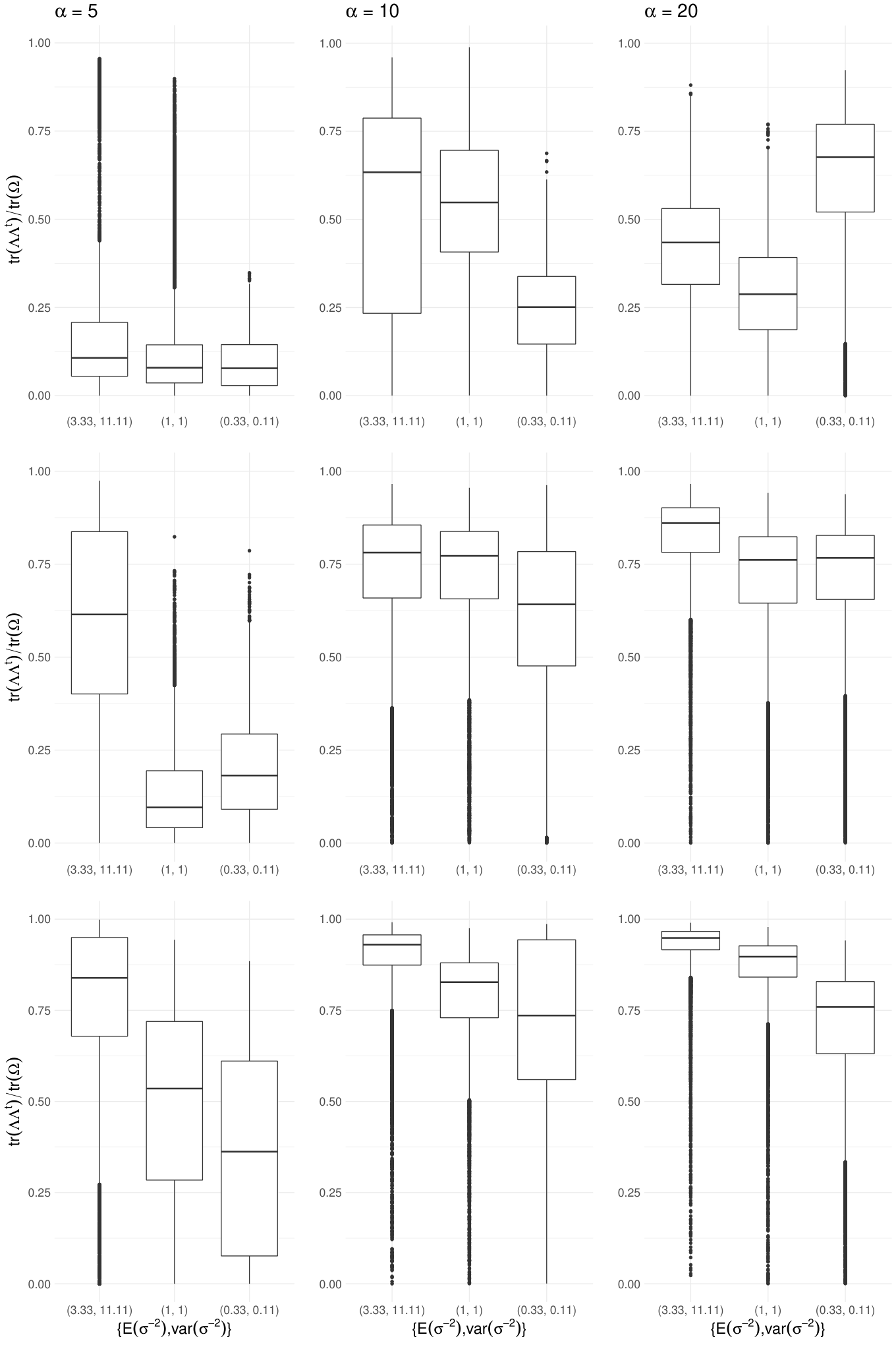
The latter comment is confirmed by the study of the impact of and on the posterior bound of the truncation error and on the posterior distribution of the proportion of variance explained by the factor model. Specifically, we generate synthetic data sets with observations with dimension from the Gaussian linear factor model , with a sparse matrix with . We randomly set two thirds of the elements of equal to zero, drawing the non zero elements from a Gaussian distribution with mean zero and variances sampled from an inverse gamma distribution . We keep the number of active factors fixed at , and set and . We run the Gibbs algorithm for the structured increasing shrinkage model for 15000 iterations, discarding the first 5000 iterations. Then, we thin the Markov chain, saving every 5-th sample.
In Figure S9 the sampled posterior distribution of the proportion of variance explained by the factor model is reported for varying and . The same proportion computed on the matrices generating the data is , with . A sufficiently concentrated prior on a large value of seems more suitable to model such data, even if we have incorrect expectations on the number of factors, i.e. set small.
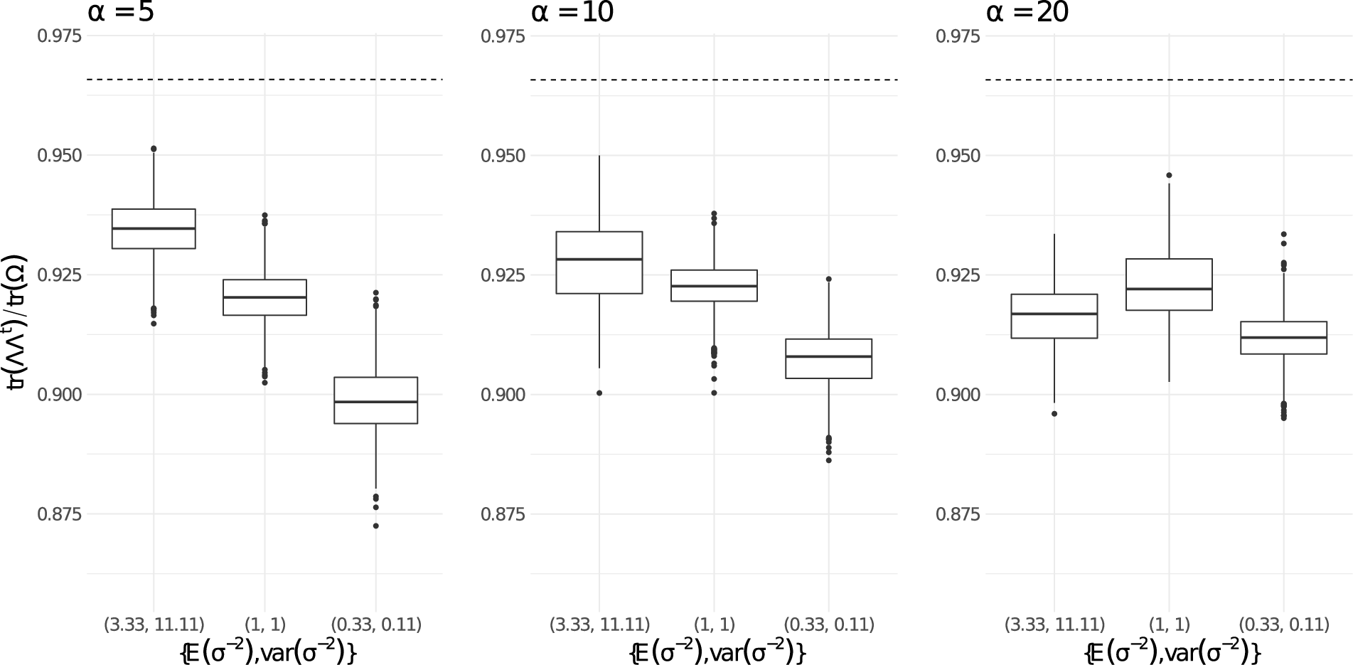
Figure S10 displays the Monte Carlo approximation of the posterior probability of truncation error for different values of and and varying and . If is sparse, a small value of induces good approximations even with smaller than the true number of factors. The inferred sparsity pattern in is robust to the prior distribution for .
Appendix S3 Finnish bird co-occurrence application
S3.1 Gibbs algorithms of probit structured increasing shrinkage model
In case of probit data (see Section 5 of the main paper) and the structured increasing shrinkage process, we can rewrite the latent model for as
where is an absolutely continuous random variable. Let the notation denote the full conditional distribution of conditionally on everything else. Given the number of factors of the truncated model, the sampler cycles through the following steps.
Step S1. Update , for every by sampling from the independent full conditional posterior distributions
where and .
Step S2. Update () sampling from conditionally independent posteriors
where
Step S3. Update the elements (; ) sampling independently from the truncated normal
where the lower bound is equal to if and otherwise. The upper bound if and otherwise. Then, set .
Step S4. Update, for , the factor according to the posterior full conditional
Step S5.
Update () exploiting the Pólya-Gamma data-augmentation strategy (Polson et al. 2013) and the decompostition , with independent a priori and distributed as Ber and Ber, respectively.
Substep S5.1. Update , for and , setting if and sampling from the full conditional distribution
if .
Substep S5.2.
Let indicate the probability density function of a Pólya-Gamma distributed random variable .
For each , generate independent random variables sampling from the full conditional distribution .
Let denote the diagonal matrix with entries ().
Substep S5.3. Define the diagonal matrix . For each , update sampling from
where is the -dimensional vector with the -th entry equal to .
Step S6. Update the elements by sampling from the independent full conditional posterior distributions of the rows vector , for ,
where is the matrix such that the generic element is , and . Set .
Step S7.
Update the column scales (for ), following the substeps below and setting .
Consistently with Legramanti et al. 2020, define the independent indicators () with prior .
Substep S7.1. Update the augmented data by sequentially sampling from the full conditional distribution
| (11) |
The mean values and are defined according to .
Set if , else .
Substep S7.2.
For , update sampling from
.
Substep S7.3. For , sample from
set and update , for .
Step S8. Update the local scales, independently for and sequentially over , by sampling from the full conditional distributions
with .
The results reported in Section 5 are obtained running the algorithm for 40000 iterations discarding the first 20000 iterations. Then, we thin the Markov Chain, saving every -th sample. We adapt the number of active factors at iteration with probability and, given the high value of considered, we choose the offset constant which belongs to for every .
S3.2 Gibbs chains mixing
S3.3 Figures

