Constrained Radar Waveform Design for Range Profiling

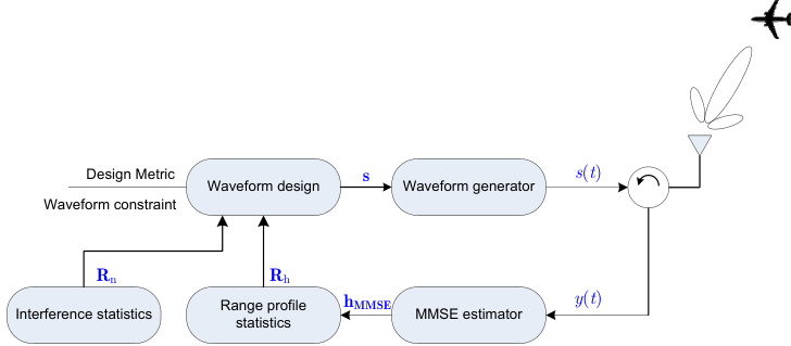
As illustrated in Fig. 1, we consider a wideband radar system with $s(t)$ being its baseband transmit waveform. Let $h(t)$ denote the TIR. Then the down-converted received signal can be written as

where $\tau_{1}$ and $\tau_{2}$ denotes the minimum and maximum two-way propagation delays, respectively, and $n(t)$ denotes the disturbance in the receiver (accounting for possible jamming signals and receiver noise). To facilitate the following discussions, we consider the discretized signal model. Let ${\mathbf{s}}=[s_{1},s_{2},\cdots,s_{L}]^{T}\in\mathbb{C}^{L}$ denote the (discrete-time) waveform (associated with $s(t)$), and ${\mathbf{h}}\in\mathbb{C}^{P}$ denote the target response vector (associated with $h(t)$), where $L$ is the code length, and $P$ is the number of range cells with target signals ¹¹ 1 $P\approx B(\tau_{2}-\tau_{1})$, where $B$ is the bandwidth of the signal.. Then the digital received signal, denoted by ${\mathbf{y}}$, can be written as

where ${\mathbf{n}}\in\mathbb{C}^{L_{0}}$ denotes the samples corresponding to $n(t)$, and $L_{0}=L+P-1$.

Define

Then ${\mathbf{y}}$ can be rewritten as

Note that similar signal models are considered in [14, 15, 26, 27]. In these papers, the authors assumed that the TIR is known a priori or partially known. The assumption is justified if a template library containing TIR at all relevant target aspect angles is available, or the radar system is cognitive, i.e., the radar system can obtain the prior knowledge of the TIR from the previous estimates (see, e.g., [28, 24, 29, 30] and the references therein for a recent discussion). Different from [14, 15, 26, 27], which used a deterministic TIR model, we employ a stochastic TIR model. Specifically, we assume that ${\mathbf{h}}\sim\mathcal{CN}(\boldsymbol{\mu}_{\textrm{h}},{\mathbf{R}}_{\textrm{h}})$, where $\boldsymbol{\mu}_{\textrm{h}}$ indicates the prior knowledge of the target response and ${\mathbf{R}}_{\textrm{h}}$ accounts for the uncertainty in the prior knowledge (${\mathbf{R}}_{\textrm{h}}$ can be estimated based on multiple previous estimates, or specified by the user). In addition, we assume that the disturbance ${\mathbf{n}}$ obeys a Gaussian distribution with zero mean and covariance matrix ${\mathbf{R}}_{\textrm{n}}$ (estimated based on target-free samples). Based on the two assumptions, we have ${\mathbf{y}}\sim\mathcal{CN}({\mathbf{S}}\boldsymbol{\mu}_{\textrm{h}},{\mathbf{R}}_{\mathbf{s}})$, where ${\mathbf{R}}_{\mathbf{s}}={\mathbf{S}}{\mathbf{R}}_{\textrm{h}}{\mathbf{S}}^{\dagger}+{\mathbf{R}}_{\textrm{n}}$.

Next we present two metrics for designing waveforms to improve the range profiling performance.

The mutual information between ${\mathbf{y}}$ and ${\mathbf{h}}$ is given by

where $\textsf{H}({\mathbf{y}})$ denotes the differential entropy of ${\mathbf{y}}$, and $\textsf{H}({\mathbf{y}}|{\mathbf{h}})$ denotes the conditional differential entropy of ${\mathbf{y}}$ given ${\mathbf{h}}$ [31]. Thus, the waveform design problem based on maximizing mutual information can be formulated as follows:

where $\mathcal{S}$ denotes the feasibility region of ${\mathbf{s}}$, and is determined by the constraints on the waveforms (detailed in Subsection II-D).

Given the signal model in (10), the MMSE estimator of ${\mathbf{h}}$ is given by [32]

The associated MMSE is

where the third equality is derived using the matrix inversion lemma [33]. Thus, the waveform design problem based on minimizing MMSE is equivalent to

In this paper, we consider the following constraints:

• •

  Energy constraint. In practical radar systems, the available transmit energy for the waveform is limited. Thus, we impose the following constraint:

  $${\mathbf{s}}^{\dagger}{\mathbf{s}}\leq e_{t},$$

  (16)

  where $e_{t}$ is the total available transmit energy. It can be proved that the mutual information is increasing and the MMSE is decreasing with respect to (w.r.t.) the waveform energy (see Appendix A for a proof). Thus, the optimal waveform maximizing the mutual information and the optimal waveform minimizing the MMSE must satisfy

  $${\mathbf{s}}^{\dagger}{\mathbf{s}}=e_{t}.$$

  (17)

• •

  PAPR constraint. To improve the efficiency of the radio frequency amplifier and avoid the nonlinear effect in the transmitter, waveforms with low PAPR is desired [34, 35, 36, 37, 38, 39, 40]. To control the PAPR of the waveform, we consider the following constraint:

  $${\mathbf{s}}^{\dagger}{\mathbf{s}}=e_{t},\textrm{PAPR}({\mathbf{s}})\leq\rho,$$

  (18)

  where $1\leq\rho\leq L$, and

  $$\textrm{PAPR}({\mathbf{s}})=\frac{\max_{l}|s(l)|^{2}}{\frac{1}{L}\sum_{l=1}^{L}|s(l)|^{2}}.$$

  (19)

  If $\rho=1$, the PAPR constraint becomes the constant-modulus constraint, i.e., the constraint in (18) can be expressed as

  $$|s(l)|=a_{s},l=1,\cdots,L,$$

  (20)

  where $a_{s}=\sqrt{e_{t}/L}$. If $\rho=L$, the constraint $\textrm{PAPR}({\mathbf{s}})\leq\rho$ is redundant and the PAPR constraint becomes the energy constraint.

• •

  Spectral constraint. The increasing demand of a larger bandwidth for radar and communication systems results in a crowded spectrum and mutual interference [41, 42, 43, 44, 39, 29]. To improve the performance and reduce the interference for a radar operating in spectrally crowded environments, we enforce a spectral constraint on the waveform (see a similar constraint in [43, 45, 46, 39]):

  $${\mathbf{s}}^{\dagger}{\mathbf{s}}=e_{t},{\mathbf{s}}^{\dagger}{\mathbf{R}}_{\textrm{I}}{\mathbf{s}}\leq E_{\textrm{I}},$$

  (21)

  where $E_{\textrm{I}}$ is the maximum allowed interference that can be tolerated by the communication systems, ${\mathbf{R}}_{\textrm{I}}=\sum_{k=1}^{K_{\textrm{rad}}}w_{k}{\mathbf{R}}_{\textrm{I},k}$, ${K_{\textrm{rad}}}$ is the number of nearby communication systems, $w_{k}$ is the weight corresponding to the $k$th communication system (which is a user-defined parameter and represents different emphasis on various communication systems),

  $${\mathbf{R}}_{\textrm{I},k}(m,n)=\begin{cases}f_{2}^{k}-f_{1}^{k},&m=n\\ \frac{e^{j2\pi f_{2}^{k}(m-n)}-e^{j2\pi f_{1}^{k}(m-n)}}{j2\pi(m-n)}&m\neq n,\end{cases}$$

  $f_{2}^{k}$ and $f_{1}^{k}$ are the upper and the lower normalized frequencies of the $k$th communication system, respectively. Note that $f_{2}^{k}$ and $f_{1}^{k}$ can be obtained from spectral regulations, or by spectrum sensing (e.g., by a cognitive radar [43, 29]).

Note that the objective function in (II-B) can be rewritten as

where we have used the fact that $\det({\mathbf{I}}+{\mathbf{A}}{\mathbf{B}})=\det({\mathbf{I}}+{\mathbf{B}}{\mathbf{A}})$ [33]. Using the matrix inversion lemma yields [33]

where ${\mathbf{K}}=[{\mathbf{I}}_{P},{\mathbf{0}}_{P\times L_{0}}]$, and

Thus, we have

It follows from Lemma 1 of [49] that $\log\det({\mathbf{K}}{\mathbf{M}}^{-1}{\mathbf{K}}^{\dagger})$ is a convex function of ${\mathbf{M}}$. Since convex functions are minorized by their supporting hyperplanes [50], we have

where

is the gradient of $\log\det({\mathbf{K}}{\mathbf{M}}^{-1}{\mathbf{K}}^{\dagger})$ at ${\mathbf{M}}_{k}$ (which can be verified by using the results from [51]),

${\mathbf{R}}_{{\mathbf{s}},k}={\mathbf{S}}_{k}{\mathbf{R}}_{\textrm{h}}{\mathbf{S}}_{k}^{\dagger}+{\mathbf{R}}_{\textrm{n}}$, and ${\mathbf{S}}_{k}$ is formed by ${\mathbf{s}}_{k}\in\mathcal{S}$ (which is the waveform at the $k$th iteration).

Let us partition ${\mathbf{G}}_{k}$ as

where ${\mathbf{G}}_{k}^{11}\in\mathbb{C}^{P\times P}$, ${\mathbf{G}}_{k}^{12}=({\mathbf{G}}_{k}^{21})^{\dagger}\in\mathbb{C}^{P\times L_{0}}$, and ${\mathbf{G}}_{k}^{22}\in\mathbb{C}^{L_{0}\times L_{0}}$. Define ${\mathbf{L}}=[{\mathbf{0}}_{L_{0}\times P},{\mathbf{I}}_{L_{0}}]$. Then we have

Using the matrix inversion lemma and after some algebraic manipulations, ${\mathbf{G}}_{k}^{22}$ can be simplified into

Using the partition of ${\mathbf{G}}_{k}$ in (29), we have

Thus, $f_{\textrm{I}}({\mathbf{s}})$ is minorized by

where $c_{\textrm{I}}={\textrm{tr}}({\mathbf{G}}_{k}^{11})+{\textrm{tr}}({\mathbf{G}}_{k}^{22}{\mathbf{R}}_{\textrm{n}})+\log\det({\mathbf{K}}{\mathbf{M}}_{k}^{-1}{\mathbf{K}}^{\dagger})-{\textrm{tr}}({\mathbf{G}}_{k}{\mathbf{M}}_{k})$.

The minorized problem under the energy constraint can be formulated as follows:

Note that ${\mathbf{A}}_{\textrm{O},k}\preceq{\mathbf{0}}$ (We refer to Appendix D for the proof). Thus, the optimization problem in (IV-A) is convex, meaning that its globally optimal solution can be found with polynomial time (e.g., via interior point method). In addition, we can derive a semi-closed-form expression of the optimal solution by using the method of Lagrange multipliers. To this end, let the Lagrangian associated with (IV-A) be

where $\mu\geq 0$ is the Lagrange multiplier associated with the energy constraint. According to the Karush-Kuhn-Tucker (KKT) conditions [50], the optimal solution of (IV-A) satisfies

if $\mu_{k}\neq 0$, then

where $\mu_{k}$ can be obtained by solving ${\mathbf{a}}_{\textrm{O},k}^{\dagger}(\mu_{k}{\mathbf{I}}-{\mathbf{A}}_{\textrm{O},k})^{-2}{\mathbf{a}}_{\textrm{O},k}=e_{t}$. Otherwise, the optimal solution is given by ${\mathbf{s}}=-{\mathbf{A}}_{\textrm{O},k}^{-1}{\mathbf{a}}_{\textrm{O},k}$.

The minorized problem under the PAPR constraint is equivalent to

We can also tackle the problem in (IV-B) by MM. To this end, we note that

where ${\mathbf{A}}_{\textrm{pos},k}={\mathbf{A}}_{\textrm{O},k}-\lambda_{\min}({\mathbf{A}}_{\textrm{O},k}){\mathbf{I}}$, $\lambda_{\min}({\mathbf{A}}_{\textrm{O},k})$ is the smallest eigenvalue of ${\mathbf{A}}_{\textrm{O},k}$, $\textrm{const}_{j}=2\lambda_{\min}({\mathbf{A}}_{\textrm{O},k})e_{t}-{\mathbf{s}}_{j}^{\dagger}{\mathbf{A}}_{\textrm{O},k}{\mathbf{s}}_{j}$, and ${\mathbf{s}}_{j}$ is the solution at the $j$th (inner) iteration. As a result, the objective function in (IV-B) is minorized by

where ${\mathbf{t}}_{k,j}={\mathbf{a}}_{\textrm{O},k}+{\mathbf{A}}_{\textrm{pos},k}{\mathbf{s}}_{j}$. Thus, the maximization problem of an MM algorithm based on (49) is

The above optimization problem can be solved by Algorithm 2 in [52]. In particular, if $\rho=1$, a closed-form expression for the optimal solution can be derived as

where $\phi_{t,l}=\arg(t_{l})$, and $t_{l}$ is the $l$th element of ${\mathbf{t}}_{k,j}$.

Algorithm 1 summarizes the procedure to tackle the PAPR-constrained optimization problem in (IV-B).

The minorized problem under the spectral constraint is given by

The optimization problem in (IV-C) is hidden-convex. Thus, it can be solved by semi-definite relaxation followed by a rank-one decomposition [53]. However, the computational complexity of solving a semi-definite programming problem is high ($O(L^{4.5})$, given that the primal-dual path following method is used). We propose using the alternating direction method of multipliers (ADMM) [54] to reduce the computational complexity (As shown in Table I, the proposed ADMM has a complexity of $O(L^{3})$). To apply the ADMM algorithm to this problem, we use the variable splitting trick and introduce an auxiliary variable ${\mathbf{u}}$ as follows:

where $\bar{{\mathbf{A}}}_{\textrm{O},k}=-{{\mathbf{A}}}_{\textrm{O},k}$, and $\bar{{\mathbf{a}}}_{\textrm{O},k}=-{{\mathbf{a}}}_{\textrm{O},k}$. The augmented Lagrangian associated with the optimization problem in (IV-C) can be written as

where $\boldsymbol{\lambda}$ is the Lagrange multiplier, and $\varrho$ is the penalty parameter. The ADMM method consists of the following iterations:

The optimization problem in (55a) can be rewritten as

where ${{\mathbf{b}}}_{\textrm{O},k}=\bar{{\mathbf{a}}}_{\textrm{O},k}+\boldsymbol{\lambda}_{j}-\varrho{\mathbf{u}}_{j}$. The optimal solution of (IV-C) can be obtained similarly to that in (IV-A):

where $\alpha_{1}$ is a scalar making ${\mathbf{s}}_{j+1}^{\dagger}{\mathbf{s}}_{j+1}=e_{t}$.

The optimization problem in (55b) is equivalent to

where ${\mathbf{d}}_{j}={\mathbf{s}}_{j+1}+\boldsymbol{\lambda}_{j}/\varrho$. Its solution is given by (see [55] for more details):

where $\alpha_{2}$ can be obtained by solving ${\mathbf{d}}_{j}^{\dagger}{\mathbf{T}}_{\textrm{I}}{\mathbf{d}}_{j}=E_{\textrm{I}}$, and ${\mathbf{T}}_{\textrm{I}}=({\mathbf{I}}+\alpha_{2}{\mathbf{R}}_{\textrm{I}})^{-1}{\mathbf{R}}_{\textrm{I}}({\mathbf{I}}+\alpha_{2}{\mathbf{R}}_{\textrm{I}})^{-1}$.

Algorithm 2 summarizes the proposed ADMM algorithm for (IV-C), where we terminate the ADMM algorithm if both the (Euclidian) norm of the primal residual ${\mathbf{r}}_{j}$ and the dual residual ${\mathbf{d}}_{j}$ are sufficiently small, where ${\mathbf{r}}_{j}={\mathbf{s}}_{j}-{\mathbf{u}}_{j}$, and ${\mathbf{d}}_{j}=\varrho({\mathbf{s}}_{j}-{\mathbf{s}}_{j+1})$.

We summarize the proposed algorithm framework in Algorithm 3. Note that in some applications, to control the shape of the ambiguity function or achieve some desired property, one needs to enforce a similarity constraint on the waveform [56], which can be written as

where ${\mathbf{s}}_{0}$ denotes a reference waveform possessing certain desirable property, ${\mathbf{s}}_{0}^{\dagger}{\mathbf{s}}_{0}=e_{t}$, and $\varepsilon_{2}$ is a user specified similarity parameter ($0\leq\varepsilon_{2}\leq 2e_{t}$). One can also enforce both constant-modulus and similarity constraints on the waveform [34, 39]. The associated constraints are given by

where the reference waveform ${\mathbf{s}}_{0}$ is constant-modulus, and $\varepsilon_{\infty}$ denotes a similarity parameter ($0\leq\varepsilon_{\infty}\leq 2a_{s}$). It can be verified that the proposed framework can be applied to deal with both the constraints in (60) and (61). Nevertheless, we omit the details here due to space limitations.

Next we analyze the convergence of the proposed algorithm. Note that $f_{\textrm{O}}({\mathbf{s}}_{k+1})\geq g_{\textrm{O}}({\mathbf{s}}_{k+1};{\mathbf{s}}_{k})$ and $f_{\textrm{O}}({\mathbf{s}}_{k})=g_{\textrm{O}}({\mathbf{s}}_{k};{\mathbf{s}}_{k})$. Thus, if $g_{\textrm{O}}({\mathbf{s}}_{k+1};{\mathbf{s}}_{k})\geq g_{\textrm{O}}({\mathbf{s}}_{k};{\mathbf{s}}_{k})$, then $f_{\textrm{O}}({\mathbf{s}}_{k+1})\geq f_{\textrm{O}}({\mathbf{s}}_{k})$, and the convergence of the sequence of the objective values is guaranteed. For the energy constraint, $g_{\textrm{O}}({\mathbf{s}}_{k+1};{\mathbf{s}}_{k})\geq g_{\textrm{O}}({\mathbf{s}}_{k};{\mathbf{s}}_{k})$ owing to the optimality of ${\mathbf{s}}_{k+1}$ given ${\mathbf{s}}_{k}$; for the PAPR constraint, if ${\mathbf{s}}_{k}$ is used as the starting point of the proposed MM method, the improvement of $g_{\textrm{O}}({\mathbf{s}}_{k+1};{\mathbf{s}}_{k})$ over $g_{\textrm{O}}({\mathbf{s}}_{k};{\mathbf{s}}_{k})$ can be verified by using the ascent property of the MM method; for the spectral constraint, if ${\mathbf{s}}_{k+1}$ is obtained by the SDR and rank-one decomposition, ${\mathbf{s}}_{k+1}$ is the optimal solution given ${\mathbf{s}}_{k}$, and it can be checked that $g_{\textrm{O}}({\mathbf{s}}_{k+1};{\mathbf{s}}_{k})\geq g_{\textrm{O}}({\mathbf{s}}_{k};{\mathbf{s}}_{k})$. Otherwise, if ${\mathbf{s}}_{k+1}$ is obtained by the proposed ADMM method, it is non-trivial to prove the optimality of ${\mathbf{s}}_{k+1}$. However, for the proposed ADMM algorithm, we do not encounter any convergence problem during the numerical simulations (possibly because of the hidden convexity of the problem in (IV-C)).

Table I summarizes the per-iteration computational complexity of the proposed algorithms, where $N_{papr}$ is the number of (inner) iterations needed to reach convergence under the PAPR constraint, and $N_{spectral}$ is the number of (inner) iterations needed to reach convergence under the spectral constraint. Note that we have ignored the computational complexity that can be performed offline (e.g., the calculation of ${\mathbf{R}}_{\textrm{n}}^{-1}$). In addition, we ignore the computational complexity involving the multiplication of ${\mathbf{E}}$, since it can be done by addition.

References

- [1] D. R. Wehner, High resolution radar. Norwood: Artech House, 1995.
- [2] P. Tait, Introduction to radar target recognition. London: The Institution of Electronic Technology, 2005.
- [3] N. Levanon, “Cross-correlation of long binary signals with longer mismatched filters,” IEE Proceedings-Radar, Sonar and Navigation, vol. 152, no. 6, pp. 377–382, 2005.
- [4] P. Stoica, J. Li, and M. Xue, “Transmit codes and receive filters for radar,” IEEE Signal Process. Mag., vol. 25, no. 6, pp. 94–109, 2008.
- [5] S. M. H. Song, W. M. Kim, P. Dongwook, and K. Young-Sik, “Estimation theoretic approach for radar pulse compression processing and its optimal codes,” Electronics Letters, vol. 36, no. 3, pp. 250–252, 2000.
- [6] S. D. Blunt and K. Gerlach, “Adaptive pulse compression via MMSE estimation,” IEEE Trans. Aerosp. Electron. Syst., vol. 42, no. 2, pp. 572–584, 2006.
- [7] H. Kikuchi, E. Yoshikawa, T. Ushio, F. Mizutani, and M. Wada, “Adaptive pulse compression technique for X-Band phased array weather radar,” IEEE Geoscience and Remote Sensing Letters, vol. 14, no. 10, pp. 1810–1814, 2017.
- [8] T. Yardibi, J. Li, P. Stoica, M. Xue, and A. B. Baggeroer, “Source localization and sensing: A nonparametric iterative adaptive approach based on weighted least squares,” IEEE Trans. Aerosp. Electron. Syst., vol. 46, no. 1, pp. 425–443, 2010.
- [9] H. He, J. Li, and P. Stoica, Waveform design for active sensing systems: a computational approach. Cambridge University Press, 2012.
- [10] F. Gini, A. De Maio, and L. Patton, Waveform design and diversity for advanced radar systems. London: Institution of engineering and technology, 2012.
- [11] G. Cui, A. De Maio, A. Farina, and J. Li, Radar Waveform Design Based on Optimization Theory. London: SciTech Publishing, 2020.
- [12] P. Stoica, H. He, and J. Li, “New algorithms for designing unimodular sequences with good correlation properties,” IEEE Trans. Signal Process., vol. 57, no. 4, pp. 1415–1425, 2009.
- [13] J. Song, P. Babu, and D. P. Palomar, “Optimization methods for designing sequences with low autocorrelation sidelobes,” IEEE Trans. Signal Process., vol. 63, no. 15, pp. 3998–4009, 2015.
- [14] D. A. Garren, A. Odom, M. Osborn, J. S. Goldstein, S. Pillai, and J. Guerci, “Full-polarization matched-illumination for target detection and identification,” IEEE Trans. Aerosp. Electron. Syst., vol. 38, no. 3, pp. 824–837, 2002.
- [15] X. Cheng, A. Aubry, D. Ciuonzo, A. D. Maio, and X. Wang, “Robust waveform and filter bank design of polarimetric radar,” IEEE Trans. Aerosp. Electron. Syst., vol. 53, no. 1, pp. 370–384, 2017.
- [16] D. Ciuonzo, A. De Maio, G. Foglia, and M. Piezzo, “Intrapulse radar-embedded communications via multiobjective optimization,” IEEE Trans. Aerosp. Electron. Syst., vol. 51, no. 4, pp. 2960–2974, 2015.
- [17] B. Tang and J. Tang, “Joint design of transmit waveforms and receive filters for MIMO radar space-time adaptive processing,” IEEE Trans. Signal Process., vol. 64, no. 18, pp. 4707–4722, 2016.
- [18] B. Tang, J. Tuck, and P. Stoica, “Polyphase waveform design for MIMO radar space time adaptive processing,” IEEE Trans. Signal Process., vol. 68, pp. 2143–2154, 2020.
- [19] M. R. Bell, “Information theory and radar waveform design,” IEEE Trans. Inf. Theory, vol. 39, no. 5, pp. 1578–1597, 1993.
- [20] A. Leshem, O. Naparstek, and A. Nehorai, “Information theoretic adaptive radar waveform design for multiple extended targets,” IEEE Journal of Selected Topics in Signal Processing, vol. 1, no. 1, pp. 42–55, 2007.
- [21] R. A. Romero, J. Bae, and N. A. Goodman, “Theory and application of SNR and mutual information matched illumination waveforms,” IEEE Trans. Aerosp. Electron. Syst., vol. 47, no. 2, pp. 912–927, 2011.
- [22] K.-W. Huang, M. Bicǎ, U. Mitra, and V. Koivunen, “Radar waveform design in spectrum sharing environment: Coexistence and cognition,” in IEEE Radar Conference (RadarCon), 2015, pp. 1698–1703.
- [23] M. Bicǎ, K.-W. Huang, V. Koivunen, and U. Mitra, “Mutual information based radar waveform design for joint radar and cellular communication systems,” in IEEE International Conference on Acoustics, Speech and Signal Processing (ICASSP). IEEE, 2016, pp. 3671–3675.
- [24] R. Palamá, H. Griffiths, and F. Watson, “Joint dynamic spectrum access and target-matched illumination for cognitive radar,” IET Radar, Sonar & Navigation, vol. 13, no. 5, pp. 750–759, 2019.
- [25] B. Tang and J. Li, “Spectrally constrained MIMO radar waveform design based on mutual information,” IEEE Trans. Signal Process., vol. 67, no. 3, pp. 821–834, 2019.
- [26] S. M. Karbasi, A. Aubry, A. De Maio, and M. H. Bastani, “Robust transmit code and receive filter design for extended targets in clutter,” IEEE Trans. Signal Process., vol. 63, no. 8, pp. 1965–1976, 2015.
- [27] B. Tang and J. Tang, “Robust waveform design of wideband cognitive radar for extended target detection,” in IEEE International Conference on Acoustics, Speech and Signal Processing (ICASSP), 2016, Conference Proceedings, pp. 3096–3100.
- [28] S. Z. Gurbuz, H. D. Griffiths, A. Charlish, M. Rangaswamy, M. S. Greco, and K. Bell, “An overview of cognitive radar: Past, present, and future,” IEEE Aerosp. Electron. Syst. Mag., vol. 34, no. 12, pp. 6–18, 2019.
- [29] C. P. Horne, A. M. Jones, G. E. Smith, and H. D. Griffiths, “Fast fully adaptive signalling for target matching,” IEEE Aerosp. Electron. Syst. Mag., vol. 35, no. 6, pp. 46–62, 2020.
- [30] G. E. Smith, Z. Cammenga, A. Mitchell, K. L. Bell, J. Johnson, M. Rangaswamy, and C. Baker, “Experiments with cognitive radar,” IEEE Aerosp. Electron. Syst. Mag., vol. 31, no. 12, pp. 34–46, 2016.
- [31] T. M. Cover and J. A. Thomas, Elements of information theory. New Jersey: John Wiley & Sons, 2012.
- [32] S. M. Kay, Fundamentals of Statistical Signal Processing: Estimation Theory. New Jersey: Prentice Hall, 1993.
- [33] R. A. Horn and C. R. Johnson, Matrix analysis. Cambridge: Cambridge University Press, 1990.
- [34] A. De Maio, S. De Nicola, Y. Huang, Z.-Q. Luo, and S. Zhang, “Design of phase codes for radar performance optimization with a similarity constraint,” IEEE Trans. Signal Process., vol. 57, no. 2, pp. 610–621, 2009.
- [35] A. De Maio, Y. Huang, M. Piezzo, S. Zhang, and A. Farina, “Design of optimized radar codes with a peak to average power ratio constraint,” IEEE Trans. Signal Process., vol. 59, no. 6, pp. 2683–2697, 2011.
- [36] P. Stoica, H. He, and J. Li, “Optimization of the receive filter and transmit sequence for active sensing,” IEEE Trans. Signal Process., vol. 60, no. 4, pp. 1730–1740, 2012.
- [37] M. Soltanalian, B. Tang, J. Li, and P. Stoica, “Joint design of the receive filter and transmit sequence for active sensing,” IEEE Signal Processing Letters, vol. 20, no. 5, pp. 423–426, 2013.
- [38] L. Wu, P. Babu, and D. P. Palomar, “Transmit waveform/receive filter design for MIMO radar with multiple waveform constraints,” IEEE Trans. Signal Process., vol. 66, no. 6, pp. 1526–1540, 2018.
- [39] A. Aubry, A. D. Maio, M. A. Govoni, and L. Martino, “On the design of multi-spectrally constrained constant modulus radar signals,” IEEE Trans. Signal Process., vol. 68, pp. 2231–2243, 2020.
- [40] B. Tang and P. Stoica, “Information-theoretic waveform design for MIMO radar detection in range-spread clutter,” Signal Processing, vol. 182, p. 107961, 2021.
- [41] H. Griffiths, L. Cohen, S. Watts, E. Mokole, C. Baker, M. Wicks, and S. Blunt, “Radar spectrum engineering and management: technical and regulatory issues,” Proceedings of the IEEE, vol. 103, no. 1, pp. 85–102, 2015.
- [42] M. Bockmair, C. Fischer, M. Letsche-Nuesseler, C. Neumann, M. Schikorr, and M. Steck, “Cognitive radar principles for defence and security applications,” IEEE Aerosp. Electron. Syst. Mag., vol. 34, no. 12, pp. 20–29, 2019.
- [43] V. Carotenuto, A. Aubry, A. D. Maio, N. Pasquino, and A. Farina, “Assessing agile spectrum management for cognitive radar on measured data,” IEEE Aerosp. Electron. Syst. Mag., vol. 35, no. 6, pp. 20–32, 2020.
- [44] J. Yang, A. Aubry, A. De Maio, X. Yu, and G. Cui, “Design of constant modulus discrete phase radar waveforms subject to multi-spectral constraints,” IEEE Signal Processing Letters, vol. 27, pp. 875–879, 2020.
- [45] A. Aubry, A. De Maio, M. Piezzo, and A. Farina, “Radar waveform design in a spectrally crowded environment via nonconvex quadratic optimization,” IEEE Trans. Aerosp. Electron. Syst., vol. 50, no. 2, pp. 1138–1152, 2014.
- [46] A. Aubry, V. Carotenuto, A. De Maio, A. Farina, and L. Pallotta, “Optimization theory-based radar waveform design for spectrally dense environments,” IEEE Aerosp. Electron. Syst. Mag., vol. 31, no. 12, pp. 14–25, 2016.
- [47] D. R. Hunter and K. Lange, “A tutorial on MM algorithms,” The American Statistician, vol. 58, no. 1, pp. 30–37, 2004.
- [48] Y. Sun, P. Babu, and D. P. Palomar, “Majorization-minimization algorithms in signal processing, communications, and machine learning,” IEEE Trans. Signal Process., vol. 65, no. 3, pp. 794–816, 2017.
- [49] B. Tang, Y. Zhang, and J. Tang, “An efficient minorization maximization approach for MIMO radar waveform optimization via relative entropy,” IEEE Trans. Signal Process., vol. 66, no. 2, pp. 400–411, 2018.
- [50] S. Boyd and L. Vandenberghe, Convex optimization. Cambridge: Cambridge University Press, 2004.
- [51] A. Hjorungnes and D. Gesbert, “Complex-valued matrix differentiation: Techniques and key results,” IEEE Trans. Signal Process., vol. 55, no. 6, pp. 2740–2746, 2007.
- [52] J. A. Tropp, I. S. Dhillon, R. W. Heath, and T. Strohmer, “Designing structured tight frames via an alternating projection method,” IEEE Trans. Inf. Theory, vol. 51, no. 1, pp. 188–209, 2005.
- [53] W. Ai, Y. Huang, and S. Zhang, “New results on hermitian matrix rank-one decomposition,” Mathematical programming, vol. 128, no. 1-2, pp. 253–283, 2011.
- [54] S. Boyd, N. Parikh, E. Chu, B. Peleato, and J. Eckstein, “Distributed optimization and statistical learning via the alternating direction method of multipliers,” Foundations and Trends® in Machine Learning, vol. 3, no. 1, pp. 1–122, 2011.
- [55] B. Tang, J. Li, and J. Liang, “Alternating direction method of multipliers for radar waveform design in spectrally crowded environments,” Signal Processing, vol. 142, pp. 398–402, 2018.
- [56] J. Li, J. R. Guerci, and L. Xu, “Signal waveform’s optimal-under-restriction design for active sensing,” IEEE Signal Processing Letters, vol. 13, no. 9, pp. 565–568, 2006.
- [57] P. Z. Fan, N. Suehiro, N. Kuroyanagi, and X. M. Deng, “Class of binary sequences with zero correlation zone,” Electronics Letters, vol. 35, no. 10, pp. 777–779, 1999.
- [58] Y. Yang and R. S. Blum, “MIMO radar waveform design based on mutual information and minimum mean-square error estimation,” IEEE Trans. Aerosp. Electron. Syst., vol. 43, no. 1, pp. 330–343, 2007.
- [59] Y. Gu and N. A. Goodman, “Information-theoretic waveform design for Gaussian mixture radar target profiling,” IEEE Trans. Aerosp. Electron. Syst., vol. 55, no. 3, pp. 1528–1536, 2019.
- [60] D. S. Bernstein, Matrix mathematics: theory, facts, and formulas. Princeton University Press, 2009.
- [61] J. V. Burke and T. Hoheisel, “Matrix support functionals for inverse problems, regularization, and learning,” SIAM Journal on Optimization, vol. 25, no. 2, pp. 1135–1159, 2015.