How to Compute Invariant Manifolds and their Reduced Dynamics in High-Dimensional Finite-Element Models

Shobhit Jain Note: Corresponding author: shjain@ethz.ch George Haller

Abstract

Invariant manifolds are important constructs for the quantitative and qualitative understanding of nonlinear phenomena in dynamical systems. In nonlinear damped mechanical systems, for instance, spectral submanifolds have emerged as useful tools for the computation of forced response curves, backbone curves, detached resonance curves (isolas) via exact reduced-order models. For conservative nonlinear mechanical systems, Lyapunov subcenter manifolds and their reduced dynamics provide a way to identify nonlinear amplitude-frequency relationships in the form of conservative backbone curves. Despite these powerful predictions offered by invariant manifolds, their use has largely been limited to low-dimensional academic examples. This is because several challenges render their computation unfeasible for realistic engineering structures described by finite-element models. In this work, we address these computational challenges and develop methods for computing invariant manifolds and their reduced dynamics in very high-dimensional nonlinear systems arising from spatial discretization of the governing partial differential equations. We illustrate our computational algorithms on finite-element models of mechanical structures that range from a simple beam containing tens of degrees of freedom to an aircraft wing containing more than a hundred-thousand degrees of freedom.

Institute for Mechanical Systems, ETH Zürich

Leonhardstrasse 21, 8092 Zürich, Switzerland

Keywords: Invariant manifolds, Finite Elements, Reduced-order modeling, Spectral Submanifolds, Lyapunov Subcenter manifolds, Center manifolds, Normal forms.

1 Introduction

Invariant manifolds are low-dimensional surfaces in the phase space of a dynamical system that constitute organizing centers of nonlinear dynamics. These surfaces are composed of full system trajectories that stay on them for all times, partitioning the phase space locally into regions of different behavior. For instance, invariant manifolds attached to fixed points can be viewed as the nonlinear analogues of (flat) modal subspaces of the linearized system. Classic examples are the stable, unstable and center manifolds tangent to the stable, unstable and center subspaces of fixed points (see, e.g., Guckenheimer & Holmes [1]). The most important class of invariant manifolds are those that attract other trajectories and hence their own low-dimensional internal dynamics acts a mathematically exact reduced-order model for the full, high-dimensional system. The focus of this article is to compute such invariant manifolds and their reduced dynamics accurately and efficiently in very high-dimensional nonlinear systems.

The theory of invariant manifolds has matured over more than a century of research and has been applied to numerous fields for the qualitative understanding of nonlinear behavior of systems (see Fenichel [2, 3, 4], Hirsch et al. [5], Wiggins [6], Eldering [7], Nipp & Stoffer [8]). The computation of invariant manifolds, on the other hand, is a relatively new and rapidly evolving discipline due to advances in scientific computing. In this paper, we address some challenges that have been hindering the computation of invariant manifolds in high-dimensional mechanical systems arising from spatially discretized partial differential equations (PDEs).

The methods for computing invariant manifolds can be divided into two categories: local and global. Local methods approximate an invariant manifold in the neighborhood of simpler invariant sets, such as fixed points, periodic orbits or invariant tori. Such local approximations are performed using Taylor series approximations around the fixed point or Taylor-Fourier series around the periodic orbit/invariant torus (see Simo [25]). Global methods, on the other hand, seek invariant manifolds globally in the phase space. Global techniques generally employ numerical continuation for growing invariant manifolds from their local approximation that may be obtained from the linearized dynamics (see Krauskopf et al. [10] for a survey).

Global techniques

A key aspect of most global techniques is to discretize the manifold into a mesh e.g., via a collocation or a spectral approach (see Dancowicz & Schilder [19], Krauskopf et al. [11]) and solve invariance equations for the unknowns at the mesh points. For growing an $M-$ dimensional manifold via $q$ collocation/spectral points (along each of the $M$ dimensions) in an $N-$ dimensional dynamical system, one needs to solve a system of $\mathcal{O}\left(Nq^{M}\right)$ nonlinear algebraic equations at each continuation step. This is achieved via an iterative solver such as the Newton’s method. As $N$ invariably becomes large in the case of discretized PDEs governing mechanics applications, numerical continuation of invariant manifolds via collocation and spectral approaches becomes computationally intractable. Indeed, while global approaches are often discussed for general systems, the most common applications of these approaches tend to involve low-dimensional problems, such as the computation of the Lorenz manifold (Krauskopf & Osinga [9]).

Global approaches also include the continuation of trajectory segments along the invariant manifold, expressed as a family of trajectories. This is achieved by formulating a two-point boundary value problem (BVP) satisfied by the trajectory on the manifold and numerically following a branch of solutions (see Krauskopf et al. [10], Guckenheimer et al. [49]). While collocation and spectral methods are valid means to achieve this end as well, the (multiple) shooting method method (see Keller [12], Stoer & Bulirsch [13]) has a distinguishing appeal from a computational perspective for high-dimensional problems. In the (multiple) shooting method, an initial guess for one point on the solution trajectory is iteratively corrected such until the two-point BVP is solved up to a required precision. In each iteration, one performs numerical time integration of the full nonlinear system between the two points of the BVP, which is a computationally expensive undertaking for large systems. However, time integration involves the solution $\mathcal{O}\left(N\right)$ nonlinear algebraic equations at each time step, in contrast to collocation and spectral methods which require $\mathcal{O}\left(Nq\right)$ nonlinear algebraic equations to be solved simultaneously for $q$ collocation/spectral points. Coupled with advances in domain decomposition methods for time integration (see Carraro et al. [15]), the multiple shooting method provides a feasible alternative to collocation and spectral methods. Still, covering a multi-dimensional invariant manifold using trajectory segments in a high-dimensional system is an elusive task even for multiple shooting methods (see, e.g., Jain et al. [60]).

A number of numerical continuation packages have enabled the computation of global invariant manifolds via collocation, spectral or multiple shooting methods. AUTO [16], a FORTRAN-based package, constitutes the earliest organized effort towards continuation and bifurcation analysis of parameter-dependent ODEs. AUTO [16] employs orthogonal collocation to approximate solutions and is able to continue solution families in two or three parameters. The MATLAB-based package Matcont [17] addresses some of the limitations of AUTO, albeit at a loss of computational performance. Additionally, Matcont can also perform normal form analysis. coco [19] is an extensively documented and object-oriented MATLAB package which enables continuation via multidimensional atlas algorithms (Dankowicz et al. [14]) and implements collocation as well as spectral methods. Another recent MATLAB package, NLvib [18], implements the pseudo arc-length technique for the continuation of single-parameter family of periodic orbits in nonlinear mechanical systems via the shooting method or the spectral method (commonly referred to as harmonic balance in mechanics). Similar continuation packages are also available in the context of delay differential equations (see DDE-BIFTOOL [23], written in MATLAB and Knut [24], written in C++). The main focus of all these and other similarly useful packages is to implement automated continuation procedures, including demonstrations on low-dimensional examples, but not on the computational complexity of the operations as $N$ increases. As discussed above, the collocation/spectral/shooting techniques that are invariably employed in such packages limit their ability to compute invariant manifolds in high-dimensional mechanics problems, where system dimensionality $N$ varies from several thousands to millions.

Local techniques

In contrast to global techniques, local techniques for invariant manifold computations produce approximations valid in a neighborhood of a fixed point, periodic orbit or invariant torus. As a result, local techniques are generally unable to compute homoclinic and heteroclinic connections. Nonetheless, in engineering applications, local approximations of invariant manifolds often suffice for assessing the influence of nonlinearities on a well-understood linearized response.

Center manifold computations and their associated local bifurcation analysis via normal forms (see Guckenheimer & Holmes [1]) are classic applications of local approximations where the manifold is expressed locally as a graph over the center subspace. For an $M-$ dimensional manifold, this local graph is sought via an $M-$ variate Taylor series where the coefficient of each monomial term is unknown. These unknown coefficients are determined by solving the invariance equations in a recursive manner at each polynomial order of approximation, i.e., the solution at a lower order can be computed without the knowledge of the higher-order terms. The computational procedure simply involves the solution of a system of $\mathcal{O}(N)$ linear equations for each monomial in the Taylor expansion (see Simo [25] for flows, Fuming & Küpper, [26] for maps). Thus, in the computational context of high-dimensional problems, local techniques that employ Taylor series approximations exhibit far greater feasibility in comparison to global techniques that involve the continuation of collocation, spectral or shooting based solutions.

More recently, the parametrization method has emerged as a rigorous framework for the local analysis and computation of invariant manifolds of discrete and continuous time dynamical systems. This method was first developed in papers by Cabré, Fontich & de la Llave [27, 28, 29] for invariant manifolds tangent to eigenspaces of fixed points of nonlinear mappings on Banach spaces, and then extended to whiskered tori by Haro & de la Llave [30, 32, 31]. We refer to the monograph by Haro et al. [33] for an overview of the results. An important feature of the parametrization method is that it does not require the manifold parametrization to be the graph of a function and hence allows for folds in the manifold. Furthermore, the method returns the dynamics on the invariant manifold along with its embedding. The formal computation can again be carried out via Taylor series expansions when the invariant manifold is attached to a fixed point and via Fourier-Taylor expansions when it is attached to an invariant torus perturbing from a fixed point (see, e.g., Mireles James [34], Castelli et al. [35], Ponsioen et al. [37, 42]).

The main focus of the parametrization method has been on the computer-assisted proofs of existences and uniqueness of invariant manifolds, for which the dynamical system is conveniently diagonalized at the linear level. Furthermore, as discussed by Haro et al. [33], this diagonalization allows a choice between different styles of parametrization for the reduced dynamics on the manifold, such as a normal form style, a graph style or a mixed style. Recent applications of the parametrization method include the computation of spectral submanifolds or SSMs (Haller & Ponsioen [52]) and Lyapunov subcenter manifolds or LSMs (Kelley [47]). For these manifolds the normal form parametrization style can be used to directly extract forced response curves (FRC) and backbone curves in nonlinear mechanical systems, as we will discuss in this paper (see Ponsioen et al. [37, 42], Breunung & Haller [38], Veraszto et al. [39]).

Our contributions

While helpful for proofs and expositions, the routinely performed diagonalization and the associated linear coordinate change in invariant manifold computations, render the parametrization method unfeasible to high-dimensional mechanics problems for two reasons. First, diagonalization involves the computation of all $N$ eigenvalues of an $N-$ dimensional dynamical system and second, the nonlinear coefficients in physical coordinates exhibit an inherent sparsity in mechanics applications that is annihilated by the linear coordinate change associated to diagonalization. Both these factors lead to unmanageable computation times and memory requirements when $N$ becomes large, as we discuss in Section 3 of this manuscript.

To address these issues, we develop here a new computational methodology for local approximations to invariant manifolds via the parametrization method. The key aspects making this methodology scalable to high-dimensional mechanics problems are the use of physical coordinates and just the minimum number of eigenvectors. In the autonomous setting, we seek to compute invariant manifolds attached to fixed points where we develop expressions for the Taylor series coefficients that determine the parametrization of the invariant manifold as well as its reduced dynamics in different styles of parametrization (see Section 4). We develop similar expressions in the non-autonomous periodic or quasiperiodic setting, where we seek to compute invariant manifolds or whiskers attached to an invariant torus perturbed from a hyperbolic fixed point under the addition of small-amplitude non-autonomous terms. In this case, we seek to compute the coefficients in Fourier-Taylor series that parametrize the invariant manifold as well as its reduced dynamics in different parametrization styles (see Section 5). Finally, we apply this methodology to high-dimensional examples arising from a finite-element discretization of structural mechanics problems, whose forced response curves we recover from a normal form style parametrization of SSMs (see Section 6).

Related computational ideas have already been used in other contexts. For instance, Beyn & Kleß [61] performed similar Taylor series-based computations of invariant manifolds attached to fixed points in physical coordinates using master modes. Their work predates the parametrization method and does not involve the choice of reduced dynamics or normal forms. Recently, Carini et al. [58] focused on computing center manifolds of fixed points and their normal forms using only master modes in physical coordinates. While this an application of the parametrization method in the normal form style, they attribute their results to earlier related work by Coullet & Spiegel [59] and use these center manifolds for analyzing stability of flows around bifurcating parameter values.

More recently, Vizzaccaro et al. [43] and Opreni et al. [44] have computed normal forms on second-order, proportionally-damped mechanical systems with up to cubic nonlinearities and derived explicit expressions up to cubic order accuracy (see also Touzé et al. [45] for a review). This is a direct application of the parametrization method via a normal-form style parametrization to formally compute assumed invariant manifolds whose existence/uniqueness is a priori unclear (cf. Haller & Ponsioen [52]). These results in [43, 44] provide low-order approximations to SSMs [52], whose computation up to arbitrarily high orders of accuracy has already been automated in prior work [37, 42] for mechanical systems with diagonalized linear part. A major computational advance in the approach of Vizzaccaro et al. [43] is the nonintrusive use of finite element software to compute normal form coefficients up to cubic order. All these prior results, however, are fundamentally developed for unforced (non-autonomous) systems.

The computation procedure we develop is generally applicable to first-order systems with smooth nonlinearities, periodic or quasiperiodic forcing, and enables automated computation of various types of invariant manifolds such as stable-, unstable-, and center manifolds, LSMs, and SSMs, up to arbitrarily high orders of accuracy in physical coordinates. Finally, a numerical implementation of these computational techniques is available in the form of an open-source MATLAB package, SSMTool 2.0 [69], which is integrated with a generic finite-element solver (Jain et al. [70]) for mechanics problems. We describe some key symbols and the notation used in the remainder of this paper in Table 1 before proceeding towards the technical setup in the next section.

2 General setup

Symbol	Meaning
$n$	Dimensionality of full second-order mechanical system (1)
$N$	Dimensionality of the full first-order system (2) in the first-order ( $N=2n$ for mechanical systems)
$E$	Master (spectral) subspace of a fixed point of system (2)
$\mathcal{W}(E)$	Invariant manifold tangent to $E$ at its fixed point
$M$	$\dim(E)=\dim(\mathcal{W}(E))$ : Dimensionality of the invariant manifold constructed around $E$
$\mathbf{W}:\mathbb{C}^{M}\to\mathbb{R}^{N}$	Parametrization for the invariant manifold $\mathcal{W}(E)$
$\mathbf{R}:\mathbb{C}^{M}\to\mathbb{C}^{M}$	Parametrization for the reduced dynamics on $\mathcal{W}(E)$
$\mathbf{p}\in\mathbb{C}^{M}$	Parametrization coordinates describing reduced dynamics: $\dot{\mathbf{p}}=\mathbf{R}(\mathbf{p},t)$
$(\bullet)^{\top}$	Transpose of a matrix or vector
$\bar{(\bullet)}$	Complex conjugation operation
$(\bullet)^{\star}$	Complex conjugate transpose for a matrix or vector; adjoint for an operator.
$K$	Number of rationally incommensurate forcing frequencies in system (1) or (2)
$\boldsymbol{\Omega}\in\mathbb{R}_{+}^{K}$	Quasiperiodic forcing frequencies
$\gamma_{\epsilon}$	small amplitude invariant torus of system (2)
$\mathcal{W}(E,\gamma_{\epsilon})$	Invariant manifold (whisker) of torus $\gamma_{\epsilon}$ perturbed from spectral subspace $E$ .
$\mathbf{W}_{\epsilon}:\mathbb{C}^{M}\times\mathbb{T}^{K}\to\mathbb{R}^{N}$	Parametrization for the whisker $\mathcal{W}(E,\gamma_{\epsilon})$
$\mathbf{R}_{\epsilon}:\mathbb{C}^{M}\times\mathbb{T}^{K}\to\mathbb{C}^{M}$	Parametrization for the reduced dynamics on $\mathcal{W}(E,\gamma_{\epsilon})$
$\mathbf{e}_{j}$	$[0,\dots,0,\overset{\overset{j-\mathrm{th\,position}}{\uparrow}}{1},0,\dots,0]^{\top}$ : vector aligned along the $j-$ th coordinate axis in Euclidean space
$\mathrm{vec}(\bullet)$	Vectorization operation
$\Delta_{i,M}$	An ordered set, $\{\boldsymbol{\ell}_{1},\dots,\boldsymbol{\ell}_{M^{i}}\in\{1,\dots,M\}^{i}\}$ , which contains all possible $i-$ tuples drawn from the set $\{1,\dots,M\}$ for any $i\in\mathbb{N}$
$\mathrm{i}$	imaginary unit
$\otimes$	Kronecker product

Table 1: Notation

We are mainly interested here in dynamical systems arising from mechanics problems. Such problems are governed by PDEs that are spatially discretized typically via the finite element method. The discretization results in a system of second-order ordinary differential equations for the generalized displacement $\mathbf{x}(t)\in\mathbb{R}^{n}$ , which can be written as

\mathbf{M}\ddot{\mathbf{x}}+\mathbf{C}\dot{\mathbf{x}}+\mathbf{K}\mathbf{x}+\mathbf{f}(\mathbf{x},\dot{\mathbf{x}})=\epsilon\mathbf{f}^{ext}(\mathbf{x},\dot{\mathbf{x}},\mathbf{\Omega}t).

(1)

Here $\mathbf{M},\mathbf{C},\mathbf{K}\in\mathbb{R}^{n\times n}$ are the mass, stiffness and damping matrices; $\mathbf{f}(\mathbf{x},\dot{\mathbf{x}})\in\mathbb{R}^{n}$ is the purely nonlinear internal force; $\mathbf{f}^{ext}(\mathbf{x},\dot{\mathbf{x}},\mathbf{\Omega}t)\in\mathbb{R}^{n}$ denotes the (possibly linear) external forcing with frequency vector $\mathbf{\Omega}\in\mathbb{R}^{K}$ for some $K\geq 0$ . The function $\mathbf{f}^{ext}$ is autonomous for $K=0$ , periodic in $t$ for $K=1$ , and quasi-periodic for $K>1$ with $K$ rationally incommensurate frequencies. The second-order system (1) may be expressed in a first-order form as

	$\displaystyle\mathbf{B}\dot{\mathbf{z}}$	$\displaystyle=\mathbf{Az}+\mathbf{F}(\mathbf{z})+\epsilon\mathbf{F}^{ext}(\mathbf{z},\boldsymbol{\phi}),$		(2)
	$\displaystyle\dot{\boldsymbol{\phi}}$	$\displaystyle=\boldsymbol{\Omega},$		(3)

where $\mathbf{z}=\left[\begin{array}[]{c}\mathbf{x}\\ \dot{\mathbf{x}}\end{array}\right]$ , $\mathbf{A},\mathbf{B}\in\mathbb{R}^{2n\times 2n},\text{$\mathbf{F}:\mathbb{R}^{2n}\to\mathbb{R}^{2n}$},\mathbf{F}^{ext}:\mathbb{R}^{2n}\times\mathbb{T}^{K}\to\mathbb{R}^{2n}$ denote the first-order quantities derived from system (1). Such a first-order conversion is not unique: two equivalent choices are given by (see Tisseur & Meerbergen [36])

(L1):\hskip 8.50012pt\mathbf{A}=\left[\begin{array}[]{cc}\mathbf{0}&\mathbf{\mathbf{N}}\\ \mathbf{-\mathbf{K}}&-\mathbf{C}\end{array}\right],\hskip 8.50012pt\mathbf{B}=\left[\begin{array}[]{cc}\mathbf{N}&\mathbf{0}\\ \mathbf{0}&\mathbf{M}\end{array}\right],\hskip 8.50012pt\mathbf{F}(\mathbf{z})=\left[\begin{array}[]{c}\mathbf{0}\\ -\mathbf{f}(\mathbf{x},\dot{\mathbf{x}})\end{array}\right],\hskip 8.50012pt\mathbf{F}^{ext}(\mathbf{z},\boldsymbol{\phi})=\left[\begin{array}[]{c}\mathbf{0}\\ \mathbf{f}^{ext}(\mathbf{x},\dot{\mathbf{x}},\boldsymbol{\phi})\end{array}\right],

(4)

(L2):\hskip 8.50012pt\mathbf{A}=\left[\begin{array}[]{cc}-\mathbf{K}&\mathbf{0}\\ \mathbf{0}&\mathbf{N}\end{array}\right],\hskip 8.50012pt\mathbf{B}=\left[\begin{array}[]{cc}\mathbf{C}&\mathbf{M}\\ \mathbf{N}&\mathbf{0}\end{array}\right],\hskip 8.50012pt\mathbf{F}(\mathbf{z})=\left[\begin{array}[]{c}\mathbf{-\mathbf{f}(\mathbf{x},\dot{\mathbf{x}})}\\ \mathbf{0}\end{array}\right],\hskip 8.50012pt\mathbf{F}^{ext}(\mathbf{z},\boldsymbol{\phi})=\left[\begin{array}[]{c}\mathbf{f}^{ext}(\mathbf{x},\dot{\mathbf{x}},\boldsymbol{\phi})\\ \mathbf{0}\end{array}\right],

(5)

where $\mathbf{N}\in\mathbb{R}^{n\times n}$ may be chosen as any non-singular matrix. If the matrices $\mathbf{M},\mathbf{C},\mathbf{K}$ are symmetric, then the choice of $\mathbf{N=-K}$ for $(L1)$ and $\mathbf{N}=\mathbf{M}$ for $(L2)$ results in the first-order matrices $\mathbf{A},\mathbf{B}$ being symmetric. The computation methodology we will discuss is for any first-order system of the form (2) for $\mathbf{z}\in\mathbb{R}^{N}$ . In particular, we have $N=2n$ for second-order mechanical systems of the form (1).

We first focus on the autonomous ( $\epsilon=0$ ) limit of the system (2), given by

\mathbf{B}\dot{\mathbf{z}}=\mathbf{Az}+\mathbf{F}(\mathbf{z}),

(6)

whose linearization at the fixed point $\mathbf{z}=0$ is

\mathbf{B}\dot{\mathbf{z}}=\mathbf{Az}.

(7)

The linear system (7) has invariant manifolds defined by eigenspaces of the generalized eigenvalue problem

\left(\mathbf{A}-\lambda_{j}\mathbf{B}\right)\mathbf{v}_{j}=\mathbf{0},\quad j=1,\dots,N,

(8)

where for each distinct eigenvalue $\lambda_{j}$ , there exists an eigenspace $E_{j}\subset\mathbb{R}^{N}$ spanned by the real and imaginary parts of the corresponding generalized eigenvector $\mathbf{v}_{j}\in\mathbb{C}^{N}$ . These eigenspaces are invariant for the linearized system (7) and, by linearity, a subspace spanned by any combination of eigenspaces is also invariant for the system (7). A general invariant subspace of this type is known as a spectral subspace [52] and is obtained by the direct-summation of eigenspaces as

E_{j_{1},\dots,j_{q}}=E_{j_{1}}\oplus\dots\oplus E_{j_{q}},

where $\oplus$ denotes the direct sum of vector spaces and $E_{j_{1},\dots,j_{q}}$ is the spectral subspace obtained from the eigenspaces $E_{j_{1}},\dots,E_{j_{q}}$ for some $q\in\mathbb{N}$ . Classic examples of spectral subspaces are the stable, unstable and center subspaces, which are denoted by $E^{s}$ , $E^{u}$ and $E^{c}$ and are obtained from eigenspaces associated to eigenvalues with negative, positive and zero real parts, respectively. By the center manifold theorem, these classic invariant subspaces of the linear system (7) persist as invariant manifolds under the addition of nonlinear terms in system (6). Specifically, there exist stable, unstable and center invariant manifolds $W^{s},W^{u}$ and $W^{c}$ tangent to $E^{s},E^{u}$ and $E^{c}$ at the origin $\mathbf{0}\in\mathbb{R}^{N}$ respectively. All these manifolds are invariant and $W^{s}$ and $W^{u}$ are also unique (see, e.g., Guckenheimer & Holmes [1]).

In analogy with the stable manifold $W^{s}$ , which is the nonlinear continuation of the stable subspace $E^{s}$ , a spectral submanifold (SSM) [52] is an invariant submanifold of the stable manifold $W^{s}$ that serves as the smoothest nonlinear continuation of a given stable spectral subspace of $E^{s}$ . The existence and uniqueness results for such spectral submanifolds under appropriate conditions are derived by Haller & Ponsioen [52] using the parametrization method of Cabré et al. [27, 28, 29]. The parametrization method also serves as a tool to compute these manifolds.

We are interested in locally approximating the invariant manifolds of the fixed point $\mathbf{0}\in\mathbb{R}^{N}$ of system (6) using the parametrization method. Let $\mathcal{W}(E)$ be an invariant manifold of system (6) which is tangent to a master spectral subspace $E\subset\mathbb{R}^{N}$ at the origin such that

\mathrm{dim}(E)=\mathrm{dim}\left(\mathcal{W}(E)\right)=M<N.

(9)

Let $\mathbf{V}_{E}=[\mathbf{v}_{1},\dots,\mathbf{v}_{M}]\in\mathbb{C}^{N\times M}$ be a matrix whose columns contain the (right) eigenvectors corresponding to the master modal subspace $E$ . Furthermore, we define a dual matrix $\mathbf{U}_{E}=[\mathbf{u}_{1},\dots,\mathbf{u}_{M}]\in\mathbb{C}^{N\times M}$ which contains the corresponding left-eigenvectors that span the adjoint subspace $E^{\star}$ as

\mathbf{u}_{j}^{\star}\left(\mathbf{A}-\lambda_{j}\mathbf{B}\right)=\mathbf{0},\quad j=1,\dots,M,

(10)

where we choose these eigenvectors to satisfy the normalization condition

\mathbf{u}_{i}^{\star}\mathbf{B}\mathbf{v}_{j}=\delta_{ij}\penalty\ (\textrm{Kronecker delta)}.

(11)

Using the eigenvalue problems (8)-(10), we obtain the following relations for the matrices $\mathbf{V}_{E}$ and $\mathbf{U}_{E}$

\mathbf{A}\mathbf{V}_{E}=\mathbf{B}\mathbf{V}_{E}\mathbf{\Lambda}_{E},

(12)

\mathbf{U}_{E}^{\star}\mathbf{A}=\mathbf{\Lambda}_{E}\mathbf{U}_{E}^{\star}\mathbf{B},

(13)

where $\mathbf{\Lambda}_{E}:=\mathrm{diag}(\lambda_{1},\dots,\lambda_{M})$ . We note that if the matrices $\mathbf{M},\mathbf{C},\mathbf{K}$ are symmetric, then the matrices $\mathbf{A},\mathbf{B}$ will be symmetric as well. In that case, the left and the right eigenvectors $\mathbf{u}_{j},\mathbf{v}_{j}$ are identical and we may conveniently choose $\mathbf{U}_{E}=\bar{\mathbf{V}}_{E}$ , with the overbar denoting complex conjugation.

The common approach to local invariant manifold computation involves diagonalizing the system (6) as

\displaystyle\dot{\mathbf{q}}

\displaystyle=\mathbf{\Lambda q}+\mathbf{T}(\mathbf{q}),

(14)

where

\mathbf{\Lambda}:=\mathrm{diag}(\lambda_{1},\dots,\lambda_{N}),\quad\mathbf{T}(\mathbf{q}):=\mathbf{U}^{\star}\mathbf{F}(\mathbf{V}\mathbf{q}),\quad\mathbf{V}=[\mathbf{v}_{1},\dots,\mathbf{v}_{N}],\quad\mathbf{U}=[\mathbf{u}_{1},\dots,\mathbf{u}_{N}],

(15)

and $\mathbf{q}\in\mathbb{C}^{N}$ are modal coordinates with $\mathbf{z}=\mathbf{V}\mathbf{q}$ . When $\mathbf{B}=\mathbf{I}_{N}$ , then using the normalization condition (11), we obtain $\mathbf{U}^{\star}=\mathbf{V}^{-1}$ , which results in the familiar diagonalized form (14) with $\mathbf{T}(\mathbf{q})=\mathbf{V}^{-1}\mathbf{F}(\mathbf{V}\mathbf{q})$ .

While the form (14) is very helpful for the purposes of proving the existence and uniqueness properties of invariant manifolds, it presents a computationally intractable form for the actual computation of invariant manifolds in high-dimensional finite element problems, as we will see next.

3 Pitfalls of the diagonalized form (14)

In this work, we use the Kronecker notation for expressing smooth nonlinear functions as a multi-variate Taylor series in terms of their arguments. The Kronecker product (also known as the outer/dyadic product) is commonly denoted by the symbol $\otimes$ . For a column vector $\mathbf{z}\in\mathbb{R}^{N}$ , the Kronecker product operation $\mathbf{z}\otimes\mathbf{z}$ returns the matrix $\mathbf{z}\mathbf{z}^{\top}\in\mathbb{R}^{N\times N}$ . In index notation, we write

(\mathbf{z}\otimes\mathbf{z})_{ij}=z_{i}z_{j},\quad\forall i,j\in{1,\dots,N}.

(16)

The Kronecker notation is more generally defined for obtaining the product of higher-order tensors, where a first-order tensor can be viewed as a vector, a second-order tensor, as a matrix and an order- $k$ tensor as a $k-$ dimensional array. Specifically, the Kronecker product of two tensors of orders $p$ and $q$ yields a tensor of order $p+q$ . We refer to Van Loan [53] for a concise review of the Kronecker product and its properties.

Now, the system nonlinearity $\mathbf{F}$ (see eq. (6)) can be expanded in terms of the physical coordinates $\mathbf{z}\in\mathbb{R}^{N}$ as

\mathbf{F}(\mathbf{z})=\sum_{k\in\mathbb{N}}\mathbf{F}_{k}\mathbf{z}^{\otimes k},

(17)

where $\mathbf{z}^{\otimes k}$ denotes the term $\mathbf{z}\otimes\dots\otimes\mathbf{z}$ ( $k$ -times), containing $N^{k}$ monomial terms at degree $k$ in the variables $\mathbf{z}$ . The array $\mathbf{F}_{k}\in\mathbb{R}^{N\times N^{k}}$ contains the coefficients of the nonlinearity $\mathbf{F}$ associated to each of these monomials. Similarly, the nonlinearity $\mathbf{T}$ (see eq. (14)) in modal coordinates $\mathbf{q}\in\mathbb{C}^{N}$ can be expanded as

\mathbf{T}(\mathbf{q})=\sum_{k\in\mathbb{N}}\mathbf{T}_{k}\mathbf{q}^{\otimes k}.

(18)

3.1 Eigenvalue and eigenvector computation

For local approximations of invariant manifolds around a fixed point of (6), it is commonly assumed that the complete generalized spectrum of the matrix $\mathbf{B}^{-1}\mathbf{A}$ (or generalized eigenvalues of the pair $\mathbf{A},\mathbf{\mathbf{B}}$ ) is known and that a basis in which the linear system (7) takes its Jordan canonical form is readily available (see, e.g., Simo [25], Homburg et al. [56], Tian & Yu [57], Haro et al. [33], Ponsioen et al. [37, 42]). For small to moderately-sized systems, obtaining a complete set of (generalized) eigenvalues/eigenvectors can indeed be accomplished using numerical eigensolvers, but this quickly transforms into an intractable task as the system size increases.

Refer to caption — Figure 1: Mesh for case study: We use a shell-based finite element mesh of a square plate with geometric nonlinearities, arising from von Kármán strains for performing numerical experiments (see Figures 2 and 3). The material is linear elastic with Young’s modulus $70$ GPa, density $2700$ kg/ $\mathrm{mm}^{3}$ and Poisson’s ratio $0.33.$ The plate has a thickness of $8$ mm and length is proportional to the square root of the total number of elements. This fixes the size of the elements in the mesh and avoids numerical errors that may otherwise arise in larger meshes.

While techniques in numerical linear algebra can help us determine a small subset of eigenvalues and eigenvectors for very high-dimensional systems using a variety of iterative methods (see, e.g., Golub & Van Loan [51]), obtaining a complete set of eigenvectors of such systems remains unfeasible despite the availability of modern computing tools. To emphasize this, we illustrate in Figure 2 the time and memory required for the eigenvalue computation for the finite element mesh for a square plate (see Figure 1). The purpose of this comparison is to report trends in computational complexity rather than precise numbers. To this end, we have used MATLAB across all comparisons, which may not be the fastest computing platform generally but is known to assimilate the state-of-the-art algorithms for numerical linear algebra computations (Golub & Van Der Vorst [22]).

(a)

(b)

Figure 2: Cost of computing eigenvalues and eigenvectors of an

n-

degree-of-freedom plate example (see Figure 1) for

n=

36, 120, 432, 1,632, 6,336, 24,960, 99,072. (a) Computation time and (b) memory required for obtaining all

n

eigenvalues and eigenvectors using the eig command of MATLAB compared to those for obtaining a subset of

5

smallest-magnitude eigenvalues and their associated eigenvectors using the eigs commands of MATLAB. These computations were performed on the ETH Zürich Euler cluster with

10^{5}

MB RAM. The computation of all eigenvalues in the case of

n=

99,072 degrees of freedom was manually terminated as the estimated computation time via extrapolation was found to be around 341 days.

Figure 2a shows that as the number of degrees of freedom, $n$ , increases from a few tens to approximately a hundred thousand, the computational time required for computing a full set of eigenvalues of the system grows polynomially up to almost a year. For computing a subset of eigenvalues in discretized PDEs, sparse iterative eigensolvers are used, such as the routines (e.g., Stewart [20], Lehoucq et al. [21]) implemented by the MATLAB’s eigs command (cf. direct eigensolvers implemented by the eig command). These sparse solvers are considered inefficient for nearly full or less sparse matrices. There are, therefore, two competing factors here, sparsity of the matrices and the size of the matrices. The small matrices in the beginning have very low sparsity and sparse eigensolver eigs of MATLAB is inefficient for computing eigenvalues here. Indeed, we see that computing the full set of eigenvalues for a small matrix (using the eig command) ends up being less expensive compared to computing a subset of eigenvalues. As sparsity is governed by the number of DOFs that are shared by neighboring elements relative to the total number of degrees of freedom, it increases with mesh refinement. Thus, sparse eigensolvers become more efficient as we refine the mesh initially, but after the refinement reaches an optimum value, the computation time is governed solely by the size of the matrix.

Furthermore, all these eigenvectors must be held in the computer’s active memory (RAM) in typical invariant manifold computations, which contributes towards very high memory requirements, as shown in Figure 2b. At the same time, these figures also show that a small subset of eigenvectors can be quickly computed and easily stored even for very high dimensional systems.

3.2 Unfeasible memory requirements due to coordinate-change

Aside from the cost of eigenvalue computation, invariant manifold computations typically involve local approximations via Taylor series. These are obtained by transforming the system into modal coordinates (see eq (14)), expressing the manifold locally as a graph over the master subspace, substituting the polynomial ansatz into eq. (14) and solving the invariance equations recursively at each order. While such a modal transformation results in decoupling of the governing equations at the linear level, it generally annihilates the inherent sparsity in the nonlinear terms, as shown in Figure 3a. That sparsity generally arises because only neighboring elements of the numerical mesh share coupled degrees of freedom. Due to the loss of this sparsity upon transformation to the diagonal form (14), the number of polynomial coefficients required to describe the nonlinearities increases by orders of magnitude, resulting in unfeasible memory requirements.

(a)

(b)

Figure 3: (a) Destruction of sparsity: Transforming the system (6) into (14) via the linear transformation

\mathbf{z}=\mathbf{Vq}

results in destruction of the inherent sparsity of the governing equations in physical coordinates

\mathbf{z}

, which leads to unfeasible memory (RAM) requirements for storing nonlinearity coefficients. Here, the multi-dimensional array

\mathbf{F}_{k}

and

\mathbf{T}_{k}

represent the polynomial coefficients at degree

k

for the nonlinearities

\mathbf{F}

(in physical coordinates) and

\mathbf{T}

(in modal coordinates); see eqs. (6), (14), (17) and (18). (b) Comparison of memory requirements for storing the nonlinearities

\mathbf{F}

and

\mathbf{T}

at degrees

k=2,3,4,5

in the

n-

degree-of-freedom square plate example (see Figure 1) with

n=

36, 120, 432, 1,632, 6,336, 24,960, 99,072 and phase space dimension

N=2n

Indeed, in Figure 3b, we compare the memory estimates for storing these coefficients in physical vs. modal coordinates as a function of the system’s phase space dimension $N$ . We see that even for the moderately sized meshes of the square plate example (see Figure 1) considered here, the storage requirements for the transformed coefficients reaches astronomically high values in the order of several terabytes/petabytes. At the same time, however, note that the RAM requirements for handling the same coefficients in physical coordinates are much less than a gigabyte, which is easily manageable for modern computers.

4 Computing invariant manifolds of fixed points in physical coordinates

Unlike commonly employed computational approaches [25, 56, 57, 33, 37, 41], we now describe the computation of general invariant manifolds in physical coordinates using the eigenvectors and eigenvalues associated to the master subspace $E$ only. This is motivated by the computational advantages we expect based on Figures 2 and 3.

We seek to compute an invariant manifold $\mathcal{W}\left(E\right)$ tangent to a spectral subspace $E$ at the origin of system (6). Let $\mathbf{W}:\mathbb{C}^{M}\to\mathbb{R}^{N}$ be a mapping that parametrizes the $M-$ dimensional manifold $\mathcal{W}\left(E\right)$ and let $\mathbf{p}\in\mathbb{C}^{M}$ be its parametrization coordinates. Then, $\mathbf{W}(\mathbf{p})$ provides us the coordinates of the manifold in the phase space of system (6), as shown in Figure 4. For any trajectory $\mathbf{z}(t)$ on the invariant manifold $\mathcal{W}\left(E\right)$ , we have a reduced dynamics trajectory $\mathbf{p}(t)$ in the parametrization space such that

\mathbf{\mathbf{z}}(t)=\mathbf{W}(\mathbf{p}(t)).

(19)

Let $\mathbf{R}:\mathbb{C}^{M}\to\mathbb{C}^{M}$ be a parametrization for the reduced dynamics. Then, any reduced dynamics trajectory $\mathbf{p}(t)$ satisfies

\dot{\mathbf{p}}=\mathbf{R}(\mathbf{p}).

(20)

Figure 4: Using the parametrization method, we obtain the parametrization

\mathbf{W}:\mathbb{C}^{M}\to\mathbb{R}^{N}

of an

M-

dimensional invariant manifold for the system (6) constructed around a spectral subspace

E

with

\dim(E)=\dim(\mathcal{W}(E))=M

. This manifold is tangent to

E

at the origin. Furthermore, we have the freedom to choose the parametrization

\mathbf{R}:\mathbb{C}^{M}\to\mathbb{C}^{M}

of the reduced dynamics on the manifold such that the function

\mathbf{W}

also maps the reduced system trajectories

\mathbf{p}(t)

onto the full system trajectories on the the invariant manifold, i.e.,

\mathbf{z}(t)=\mathbf{W}\left(\mathbf{p}(t)\right)

Differentiating eq. (19) with respect to $t$ and using eqs. (2) and (20), we obtain the invariance equation of $\mathcal{W}(E)$ as

\mathbf{B}\,(D\mathbf{W})\,\mathbf{R}=\mathbf{A}\mathbf{W}+\mathbf{F}\circ\mathbf{W}.

(21)

To solve this invariance equation, we need to determine the parametrizations $\mathbf{W}$ and $\mathbf{R}$ . We choose to parameterize the manifold and its reduced dynamics in the form of multivariate polynomial expansions as

\mathbf{W}(\mathbf{p})=\sum_{i\in\mathbb{N}}\mathbf{W}_{i}\mathbf{p}^{\otimes i},

(22)

\mathbf{R}(\mathbf{p})=\sum_{i\in\mathbb{N}}\mathbf{R}_{i}\mathbf{p}^{\otimes i},

(23)

where $\mathbf{W}_{i}\in\mathbb{C}^{N\times M^{i}}$ , $\mathbf{R}_{i}\in\mathbb{C}^{M\times M^{i}}$ are matrix representation of multi-dimensional arrays containing the unknown polynomial coefficients at degree $i$ for the parametrizations $\mathbf{W}$ and $\mathbf{R}$ . Furthermore, we have the expansion (17) for the nonlinearity $\mathbf{F}$ in physical coordinates, where $\mathbf{F}_{i}\in\mathbb{R}^{N\times N^{i}}$ are sparse arrays, which are straight-forward to store despite their large size (see Section 3.2).

Using the expansions (17), (22) and (23), we collect the coefficients of the multivariate polynomials in the invariance equation (21) at degree $i\geq 1$ , similarly to Ponsioen et al. [37], as

\left(\mathbf{B}D\mathbf{W}\mathbf{R}\right)_{i}=\mathbf{A}\mathbf{W}_{i}+\left(\mathbf{F}\circ\mathbf{W}\right)_{i},

(24)

where

\left(\mathbf{B}D\mathbf{W}\mathbf{R}\right)_{i}=\mathbf{B}\mathbf{W}_{1}\mathbf{R}_{i}+\mathbf{B}\text{$\sum_{j=2}^{i}$$\mathbf{W}_{j}\boldsymbol{\mathcal{R}}_{i,j}$},

(25)

with

\boldsymbol{\mathcal{R}}_{i,j}:=\sum_{k=1}^{j}\underbrace{\mathbf{I}_{M}\otimes\dots\otimes\mathbf{I}_{M}\otimes\overset{\overset{k-\mathrm{th\,position}}{\uparrow}}{\mathbf{R}_{i-j+1}}\otimes\mathbf{I}_{M}\otimes\dots\otimes\mathbf{I}_{M}}_{j-\mathrm{terms}},

(26)

and

\left(\mathbf{F}\circ\mathbf{W}\right)_{i}=\sum_{j=2}^{i}\mathbf{F}_{j}\left(\sum_{\mathbf{q}\in\mathbb{N}^{j},|\mathbf{q}|=i}\mathbf{W}_{q_{1}}\otimes\dots\otimes\mathbf{W}_{q_{j}}\right).

(27)

At leading-order, i.e., for $i=1$ , equation (24) simply yields

\mathbf{A}\mathbf{W}_{1}=\mathbf{B}\mathbf{W}_{1}\mathbf{R}_{1}.

(28)

Comparing equation (28) with the eigenvalue problem (12), we choose a solution for $\mathbf{W}_{1},\mathbf{R}_{1}$ in terms of the master modes and their eigenvalues as

\mathbf{W}_{1}=\mathbf{V}_{E},\quad\mathbf{R}_{1}=\boldsymbol{\Lambda}_{E}.

(29)

Remark 1.

The solution choice (29) for $\mathbf{W}_{1},\mathbf{R}_{1}$ is not unique. Indeed, we may choose $\mathbf{W}_{1}\in\mathbb{C}^{N\times M}$ to be any matrix whose columns span the master subspace $E$ , generally resulting in a non-diagonal $\mathbf{R}_{1}$ . Since our system is defined in the space of reals ( $\mathbb{R}$ ), a real choice of $\mathbf{W}_{1},\mathbf{R}_{1}$ allows us to choose the parametrization coordinates $\mathbf{p}$ in $\mathbb{R}^{M}$ instead of $\mathbb{C}^{M}$ . This will result in $\mathbf{W}_{i}\in\mathbb{R}^{N\times M^{i}}$ , $\mathbf{R}_{i}\in\mathbb{R}^{M\times M^{i}}$ for each $i$ , which reduces the computational memory requirements by half relative to the complex setting.

At any order $i\geq 2$ in eq. (24), we collect the terms containing the coefficients $\mathbf{W}_{i}$ on the left-hand side and the lower degree terms on the right-hand side as

\mathbf{B}\text{$\mathbf{W}_{i}\boldsymbol{\mathcal{R}}_{i,i}$}-\mathbf{A}\mathbf{W}_{i}=\mathbf{C}_{i}-\mathbf{B}\mathbf{W}_{1}\mathbf{R}_{i}

(30)

where $\boldsymbol{\mathcal{R}}_{i,i}$ is defined according to eq. (26) and

\mathbf{C}_{i}:=\left(\mathbf{F}\circ\mathbf{W}\right)_{i}-\mathbf{B}\text{$\sum_{j=2}^{i-1}$$\mathbf{W}_{j}\boldsymbol{\mathcal{R}}_{i,j}$}.

We solve (30) recursively for $i\geq 2$ by vectorizing it as (see, e.g., Van Loan [53])

\boldsymbol{\mathcal{L}}_{i}\mathbf{w}_{i}=\mathbf{h}_{i}(\mathbf{R}_{i}),

(31)

where

$\displaystyle\mathbf{w}_{i}$	$\displaystyle:=\mathrm{vec}\left(\mathbf{W}_{i}\right)\in\mathbb{C}^{NM^{i}},$	(32)
$\displaystyle\boldsymbol{\mathcal{L}}_{i}$	$\displaystyle:=\left(\boldsymbol{\mathcal{R}}_{i,i}^{\top}\otimes\mathbf{B}\right)-\left(\mathbf{I}_{M^{i}}\otimes\mathbf{A}\right)\in\mathbb{C}^{NM^{i}\times NM^{i}},$	(33)
$\displaystyle\mathbf{h}_{i}(\mathbf{R}_{i})$	$\displaystyle:=\mathrm{vec}\left(\mathbf{C}_{i}\right)-\mathbf{D}_{i}\mathrm{vec}\left(\mathbf{R}_{i}\right)$	(34)
$\displaystyle\boldsymbol{\mathcal{R}}_{i,i}$	$\displaystyle=\text{$\sum_{j=1}^{i}$$\left(\mathbf{I}_{M}\right)^{\otimes j-1}\otimes\mathbf{R}_{1}\otimes\left(\mathbf{I}_{M}\right)^{\otimes i-j}$}\in\mathbb{C}^{M^{i}\times M^{i}},\textrm{(from definition\,\eqref{eq:R_ij})}$	(35)
$\displaystyle\mathbf{D}_{i}$	$\displaystyle:=\left(\mathbf{I}_{M^{i}}\otimes\mathbf{B}\mathbf{W}_{1}\right)\in\mathbb{C}^{NM\times M^{i}}.$	(36)

In eq. (31), the matrix $\boldsymbol{\mathcal{L}}_{i}$ is often called the order $-i$ cohomological operator induced by the linear flow (7) and the master subspace $E$ on the linear space whose coefficients are homogeneous, $M-$ variate polynomials of degree $i$ (see Haro et al. [33], Murdock [50]). Hence, at any order of expansion $i$ , the entries of $\boldsymbol{\mathcal{L}}_{i}$ are completely determined using only the linear part of the full and reduced systems, i.e., via the matrices $\mathbf{A},\mathbf{B}$ and $\mathbf{R}_{1}$ (which is equal to $\boldsymbol{\Lambda}_{E}$ due to the choice (29)).

Remark 2.

For a diagonal choice of $\mathbf{R}_{1}$ (see, e.g., choice 29), the matrix $\boldsymbol{\mathcal{L}}_{i}$ has a block-diagonal structure, i.e., system (31) can be split into $M^{i}$ decoupled linear systems containing $N$ equations each. Hence, the coefficients parametrizing the manifold and its reduced dynamics can be determined independently for each monomial in $\mathbf{p}^{\otimes i}$ . This splitting of the large system (31) into smaller decoupled systems not only eases computations but also makes these computations appealing for a parallel computing, which has the potential to speed these computations up by a factor of $M^{i}$ at each order $i$ .

Note that the system (30) is under-determined in terms of the unknowns $\mathbf{W}_{i},\mathbf{R}_{i}$ . As discussed by Haro et al. [33], this underdeterminacy turns out to be an advantage, as it provides us the freedom to choose a particular style of parametrization depending on the context. When the matrix $\boldsymbol{\mathcal{L}}_{i}$ is non-singular for every $i\geq 2$ , the cohomological equations (31) have a unique solution $\mathbf{W}_{i}$ for any choice of the reduced dynamics $\mathbf{R}_{i}$ . The trivial choice

\mathbf{R}_{i}=\mathbf{0}\quad\forall i\geq 2,

(37)

leads to linear reduced dynamics. However, as we will see next, $\boldsymbol{\mathcal{L}}_{i}$ may be singular in the presence of resonances and yet system (31) may be solvable under an appropriate choice of parametrization.

4.1 Choice of parametrization

Eigenstructure of $\boldsymbol{\mathcal{L}}_{i}$

In order to choose the reduced dynamics $\mathbf{R}$ appropriately, we seek to explore the eigenstructure of $\boldsymbol{\mathcal{L}}_{i}$ in relation to that of the matrix $\boldsymbol{\mathcal{R}}_{i}$ and the generalized matrix pair $\left(\mathbf{B},\mathbf{A}\right)$ . We first derive a general result which helps us compute the eigenstructure of $\boldsymbol{\mathcal{R}}_{i}$ . For notational purposes, we introduce an ordered set $\Delta_{i}$ which contains all $i$ -tuples $\boldsymbol{\ell}_{j}$ (indexed lexicographically) taking values in the range $1,\dots,M$ , defined as

\Delta_{i,M}:=\{\boldsymbol{\ell}_{1},\dots,\boldsymbol{\ell}_{M^{i}}\in\{1,\dots,M\}^{i}\subset\mathbb{N}^{i}\}.

(38)

As an example, consider the case of $i=3$ and $M=2$ . Then, we may order the $3-$ tuples in $\Delta_{3,2}$ lexicographically as $\{(1,1,1),(1,1,2),(1,2,1),(1,2,2),(2,1,1),(2,1,2),(2,2,1),(2,2,2)\}$ , which contains $2^{3}$ elements. Essentially, each $\boldsymbol{\ell}\in\Delta_{i,M}$ corresponds to a monomial of degree $i$ in the reduced variables $\mathbf{p}\in\mathbb{C}^{M}$ , i.e., $p_{\ell_{1}}p_{\ell_{2}}\dots p_{\ell_{i}}$

At a high order $i$ for the manifold expansion, the matrix $\boldsymbol{\mathcal{R}}_{i,i}$ in eq. (30) may be high-dimensional, even though its components only involve the low-dimensional matrices $\mathbf{I}_{M}$ and $\mathbf{R}_{1}$ (see eq. (35)). Proposition 1 in Appendix A allows us to compute all the eigenvalues and eigenvectors of $\boldsymbol{\mathcal{R}}_{i,i}$ simply in terms of those of $\mathbf{R}_{1}$ . Indeed, let the eigenvalues of $\mathbf{R}_{1}^{\top}$ be given by $\lambda_{1},\dots,\lambda_{M}$ . Note that for a diagonal choice of $\mathbf{R}_{1}$ (see choice (29)), the left and right eigenvectors are simply given by the unit vectors aligned with the coordinate axes in $\mathbb{C}^{M}$ , i.e. $\mathbf{e}_{1},\dots,\mathbf{e}_{M}$ . Then, from Proposition 1, the eigenvalues and eigenvectors of $\boldsymbol{\mathcal{R}}_{i,i}^{\top}$ are given as

\lambda_{\mathbf{\boldsymbol{\ell}}}:=\lambda_{\ell_{1}}+\dots+\lambda_{\ell_{i}},\quad\mathbf{e}_{\boldsymbol{\ell}}=\mathbf{e}_{\ell_{1}}\otimes\dots\otimes\mathbf{e}_{\ell_{i}},\quad\boldsymbol{\ell}\in\Delta_{i,M}.

(39)

Furthermore, Proposition 2 in Appendix A characterizes the eigenstructure of $\boldsymbol{\mathcal{L}}_{i}$ in relation to that of the matrices $(\mathbf{B},\mathbf{A})$ and $\boldsymbol{\mathcal{R}}_{i,i}$ . From Proposition 2, we deduce that $\boldsymbol{\mathcal{L}}_{i}$ is singular whenever the resonance $\lambda_{\mathbf{\boldsymbol{\ell}}}=\lambda_{j}$ occurs for some $\boldsymbol{\ell}\in\Delta_{i,M}$ , $j\in\{1,\dots,N\}$ . In this case, the solvability of eq. (31) depends on the nature of such resonances. Hence, these resonances are distinguished into inner and outer resonances as

	$\displaystyle\textrm{Inner resonances:}\quad\lambda_{\mathbf{\boldsymbol{\ell}}}$	$\displaystyle=\lambda_{j},\quad\boldsymbol{\ell}\in\Delta_{i,M},j\in\{1,\dots,M\},$		(40)
	$\displaystyle\textrm{Outer resonances:}\quad\lambda_{\mathbf{\boldsymbol{\ell}}}$	$\displaystyle=\lambda_{j},\quad\boldsymbol{\ell}\in\Delta_{i,M},j\in\{M+1,\dots,N\}.$		(41)

Both inner and outer resonances result in the cohomological operator $\boldsymbol{\mathcal{L}}_{i}$ becoming singular. The main difference between these resonances is that the cohomological equation (30) can be solved in the presence of inner resonances by adjusting the parametrization choice of $\mathbf{R}_{i}$ so that the right-hand side of (30) belongs to $\mathrm{im(}\boldsymbol{\mathcal{L}}_{i})$ , which we will discuss shortly. In the presence of outer resonances, however, the right-hand side of equation (30) cannot be adjusted to lie in the range of the operator $\boldsymbol{\mathcal{L}}_{i}$ and, hence, system (30) has no solution. Indeed, the manifold does not exist in presence of certain outer resonances (see Cabré et al. [27], Haller & Ponsioen [52]). Haro et al. [33] refer to inner and outer resonances as internal and cross resonances, we use this terminology of Ponsioen et al. [37] as internal resonances carry a different meaning in the context of mechanics.

Next, we discuss two common choices for reduced dynamics parametrization, i.e., the normal form and the graph style parametrizations, which are useful for solving the cohomological equation (31) in the presence of inner resonances.

Normal form parametrization

Normal forms provide us tools for the qualitative and quantitative understanding of local bifurcations in dynamical systems. Normal form computations for any dynamical system involve successive near-identity coordinate transformations to simplify the transformed dynamics. The simplest form of dynamics that one can hope for is linear. In the presence of resonances, however, a transformation that linearizes the dynamics does not exist and the normal form procedure results in nonlinear dynamics that is only “as simple as possible”. This is achieved by systematically removing the nonessential terms from the Taylor series up to any given order (see, e.g., Guckenheimer & Holmes [1]).

Using the parametrization method, we can simultaneously compute the normal form parametrization for the reduced dynamics $\mathbf{R}$ along with the parametrization $\mathbf{W}$ for the manifold. As discussed earlier, in the absence of any inner resonances, the trivial choice (see eq. (37)) leads to the simplest (i.e., linear) reduced dynamics, which is automatically obtained from the normal form procedure. However, when the inner resonance relations (40) hold, then the dynamics cannot be linearized. In such cases, we can compute the essential nonlinear terms at degree $i$ following the normal form style of parametrization. This involves first projecting the invariance equation (31) onto $\mathrm{ker}(\boldsymbol{\mathcal{L}}_{i}^{\star})$ to eliminate the unknowns $\mathbf{W}_{i}$ and then solving for the essential nontrivial terms in $\mathbf{R}_{i}$ by computing a partial inverse (see Murdock [50]). In prior approaches, this is achieved by transforming the governing equations into diagonal coordinates [1, 33, 37, 42] which causes the matrix $\boldsymbol{\mathcal{L}}_{i}$ to be diagonal and hence simplifies the detection of its kernel. Here, we develop explicit expressions for the computation of normal form directly in physical coordinates using only the knowledge of the left eigenvectors $\mathbf{u}_{j}$ associated to the master subspace $E$ , as summarized below.

We focus on the case of a system with $r_{i}\in\mathbb{N}_{0}$ inner resonances and no outer resonances at order $i$ . Taking $\mathbf{D}=\mathcal{\boldsymbol{R}}_{i,i}^{\top}$ and $\mathbf{C}=\mathbf{I}_{M^{i}}$ in Proposition 2, we can directly estimate $\mathrm{ker}(\boldsymbol{\mathcal{L}}_{i}^{\star})$ using only the eigenvalues $\lambda_{j}$ and the corresponding eigenvectors of the master subspace $E$ . Specifically, the generalized eigenvalues for the matrix pair $(\mathbf{I}_{M^{i}},\mathcal{\boldsymbol{R}}_{i,i}^{\top})$ are given by $\mu_{\boldsymbol{\ell}}=\frac{1}{\lambda_{\mathbf{\boldsymbol{\ell}}}}$ with left-eigenvectors $\mathbf{e}_{\boldsymbol{\ell}}$ according to eq. (39) and with the left kernel $\mathcal{N}_{i}$ of $\boldsymbol{\mathcal{L}}_{i}$ given as

\mathcal{N}_{i}:=\mathrm{ker}(\boldsymbol{\mathcal{L}}_{i}^{\star})=\textrm{span}\left(\left(\mathbf{e}_{\boldsymbol{\ell}}\otimes\mathbf{u}_{j}\right)\in\mathbb{C}^{NM^{i}}|\text{$\lambda_{\mathbf{\boldsymbol{\ell}}}$}=\lambda_{j},\boldsymbol{\ell}\in\Delta_{i,M},j\in\{1,\dots,M\}\right).

(42)

Now, let $\mathbf{N}_{i}\in\mathbb{C}^{NM^{i}\times r_{i}}$ be a basis for $\mathcal{N}_{i}$ , which can be obtained by simply stacking the column vectors $\left(\mathbf{e}_{\boldsymbol{\ell}}\otimes\mathbf{u}_{j}\right)$ from Definition (42) that are associated to the modes with inner resonances (see eq. (40)). Then, the reduced dynamics coefficients in the normal form parametrization are chosen by projecting the invariance equation (31) onto $\mathbf{N}_{i}$ as

\mathbf{N}_{i}^{\star}\boldsymbol{\mathcal{L}}_{i}\mathbf{w}_{i}=\mathbf{N}_{i}^{\star}\mathbf{h}_{i}(\mathbf{R}_{i}).

(43)

The left-hand-side of eq. (43) is identically zero since columns of $\mathbf{N}_{i}$ belong to $\mathrm{ker}(\boldsymbol{\mathcal{L}}_{i}^{*})$ , i.e.,

\mathbf{N}_{i}^{\star}\boldsymbol{\mathcal{L}}_{i}=\mathbf{0}.

(44)

Hence, we are able to eliminate the unknowns $\mathbf{W}_{i}$ from eq. (43) to obtain

\mathbf{N}_{i}^{\star}\mathbf{D}_{i}\mathrm{vec}\left(\mathbf{R}_{i}\right)=\mathbf{N}_{i}^{\star}\mathrm{vec}\left(\mathbf{C}_{i}\right).

(45)

To solve eq. (45), we may further simplify it using the normalization (11) which results in

\displaystyle\mathbf{N}_{i}^{\star}\mathbf{D}_{i}

\displaystyle=\text{$\mathbf{E}_{i}$}^{\top},

(46)

where $\mathbf{E}_{i}\in\mathbb{R}^{M^{i+1}\times r_{i}}$ is a matrix whose columns are of the form $\left(\mathbf{e}_{\boldsymbol{\ell}}\otimes\mathbf{e}_{j}\right)$ , such that $\left(\mathbf{\boldsymbol{\ell}},j\right)$ are pairs with inner resonances, i.e., $\text{$\lambda_{\mathbf{\boldsymbol{\ell}}}$}=\lambda_{j}$ and $\mathbf{e}_{j}\in\mathbb{R}^{M}$ is the unit vector aligned along the $j^{\mathrm{th}}$ coordinate axis. Here, the columns $\left(\mathbf{e}_{\boldsymbol{\ell}}\otimes\mathbf{e}_{j}\right)$ of $\mathbf{E}_{i}$ must be arranged analogous to the columns $\left(\mathbf{e}_{\boldsymbol{\ell}}\otimes\mathbf{u}_{j}\right)$ of $\mathbf{N}_{i}$ . Using the relation (46), and noting that $\mathbf{N}_{i}$ is a Boolean matrix with $\mathbf{E}_{i}\text{$\mathbf{E}_{i}$}^{\top}=\mathbf{I}$ , we obtain the canonical solution to (45) for the coefficients $\mathbf{R}_{i}$ as

\textrm{Normal-form style:}\quad\mathrm{vec}\left(\mathbf{R}_{i}\right)=\mathbf{E}_{i}\mathbf{N}_{i}^{\star}\mathrm{vec}\left(\mathbf{C}_{i}\right).

(47)

Note that for each inner resonant pair $\left(\mathbf{\boldsymbol{\ell}},j\right)$ in the definition of $\mathcal{N}_{i}$ (42), the solution choice (47) produces non-trivial coefficients in the $j^{\mathrm{th}}$ equation of reduced dynamics (20) precisely for the monomial $p_{\ell_{1}}\dots p_{\ell_{i}}$ corresponding to an inner resonance. As a result, eq. (47) directly provides the normal form coefficients of the reduced dynamics on the manifold in physical coordinates, using only the knowledge of the master modes spanning the adjoint modal subspace $E^{\star}$ .

Remark 3.

(Near-resonances) As the resonance relations (40)-(41) are meant for the real as well as imaginary parts of the eigenvalues simultaneously, these are seldom satisfied exactly. However, in lightly damped systems (where the real parts of the eigenvalues are small), near-resonances might exist between the imaginary parts of the eigenvalues. In such cases, it is desirable to include the corresponding near-resonant modes in the normal form parametrization of the reduced dynamics otherwise it leads to small divisors (ill-conditioning) in solving system (31) and the domain of the validity of the Taylor approximation to the manifold shrinks (see, e.g., Guckenheimer & Holmes [1]).

Graph style parametrization

As the name suggests, a graph style of parametrization for the reduced dynamics is the result of expressing the manifold as a graph over the master subspace $E$ (see Haro et al [33]), as done in the graph transform method. The graph style of parametrization may be appealing in the context of center manifold computation, where an infinite number of inner resonances may arise. For instance, in a system with a two-dimensional center subspace with eigenvalues $\lambda_{1,2}=\pm\mathrm{i}\omega$ , its center manifold exhibits the inner resonances

	$\displaystyle\lambda_{1}$	$\displaystyle=\left(\ell+1\right)\lambda_{1}+\ell\lambda_{2},$		(48)
	$\displaystyle\lambda_{2}$	$\displaystyle=\ell\lambda_{1}+\left(\ell+1\right)\lambda_{2},\quad\forall\ell\in\mathbb{N}.$		(49)

In our setting, a graph style of parametrization is achieved by projecting the invariance equations (31) onto the subspace $\mathcal{G}_{i}$ defined as

\mathcal{G}_{i}:=\textrm{span}\left(\left(\mathbf{e}_{\boldsymbol{\ell}}\otimes\mathbf{u}_{j}\right)\in\mathbb{C}^{NM^{i}},\boldsymbol{\ell}\in\Delta_{i,M},j\in\{1,\dots,M\}\right).

(50)

Note that in the case of inner resonances, $\mathcal{N}_{i}\subset\mathcal{G}_{i}$ (cf. Definition (42)) and, hence, $\mathcal{G}_{i}$ includes all possible resonant subspaces at order $i$ . Then, similarly to the normal form style, we define a basis $\mathbf{G}_{i}\in\mathbb{C}^{NM^{i}\times M^{i}}$ for $\mathcal{G}_{i}$ , obtained by stacking the column vectors $\left(\mathbf{e}_{\boldsymbol{\ell}}\otimes\mathbf{u}_{j}\right)$ in the definition (50). We obtain a graph style of parametrization by projecting (31) on to $\mathcal{G}_{i}$ and equating the right-hand side to zero as

\mathbf{G}_{i}^{\star}\mathbf{h}_{i}(\mathbf{R}_{i})=\mathbf{0}.

(51)

In contrast to the normal form style (47), where only the coefficients of resonant monomials are nontrivial, we generally obtain a larger set of monomials with nontrivial coefficients in the graph style. Hence, the normal form style retains only the minimal number of nonlinear terms in the reduced that are essential for solving the invariance equation (21) at each order $i$ , whereas the graph style generally leads to more complex expressions of the reduced dynamics.

For the choice of $\mathbf{W}_{1}=\mathbf{V}_{E}$ (see eq. (29)) and the normalization condition (11), eq. (51) can be simplified to obtain the reduced dynamics coefficients in the graph style as

\textrm{Graph style:}\quad\mathbf{R}_{i}=\mathbf{U}_{E}^{\star}\mathbf{C}_{i}.

(52)

Note that eq. (52) directly provides the reduced dynamics coefficients in the graph style without the evaluation of $\mathbf{G}_{i}$ . Hence, an advantage of using the graph style parametrization relative to the normal form style is that specific inner resonances need not be identified a priori.

More generally, a combination of graph and normal form styles of parametrization may also be used depending on the problem. This is referred to as a mixed style of parametrization as discussed by Haro et al. [33]. A mixed style may be particularly appealing in the context of parameter-dependent manifold computation, where the parameters are dummy dynamic variables and the associated modes always have trivial dynamics. Thus, it is desirable to choose a graph style for the parametric modes and a normal form style for remaining master modes which may feature inner resonances (see Haro et al. [33], Murdock [50]).

Computing the parametrization coefficients $\mathbf{w}_{i}$

Once the reduced dynamics coefficients $\mathbf{R}_{i}$ (specific to the choice of parametrization style) are determined (see eqs. (47), (52)), we can compute the manifold parametrization coefficients $\mathbf{W}_{i}$ by solving eq. (30).

When the coefficient matrix $\boldsymbol{\mathcal{L}}_{i}$ is (nearly) singular in the presence of (near) resonances, numerical blow-up errors (ill-conditioning) may occur due to the small divisors that arise in solving system (30) using conventional solvers (see also Remark 3). As an alternative, we adopt a norm-minimizing solution to (30) given by

\mathbf{w}_{i}=\min_{\mathbf{x}\in\mathbb{C}^{NM^{i}},\boldsymbol{\mathcal{L}}_{i}\mathbf{x}=\mathbf{h}_{i}(\mathbf{R}_{i})}\|\mathbf{x}\|^{2},

(53)

which can be obtained using existing routines, such as the lsqminnorm in MATLAB. Other commonly used techniques in the literature include the simultaneous solution of equations (31) and (45) or (50). This involves the inversion of a bordered matrix that extends $\boldsymbol{\mathcal{L}}_{i}$ and ends up being non-singular (see, e.g., Beyn & Kleß [61], Kuznetsov [54]).

To summarize, we have developed an automated procedure for computing invariant manifolds attached to fixed points of system (6) and for choosing different styles of parametrizations for their reduced dynamics (eqs. (47), (52)) by solving invariance equations (31) in the physical coordinates and only using the eigenvectors associated to its master master spectral subspace. The open-source MATLAB package [69] automates this computational procedure. Next, we illustrate applications of this computation procedure developed so far.

4.2 Applications

Parameter-dependent center manifolds and their reduced dynamics

We illustrate the automated procedure developed above to compute the center manifold in the Lorenz system and its normal form style of reduced dynamics without performing any diagonalization and using only the modes associated to the center subspace. In the following example, we compute the $\rho$ -dependent center manifold and the normal form of the reduced dynamics to analyze the local bifurcation around $\rho=1$ (see section 3.2 in Guckenheimer & Holmes [1]). Consider the Lorenz system

$\displaystyle\dot{x}$	$\displaystyle=\sigma(y-x),$	(54)
$\displaystyle\dot{y}$	$\displaystyle=\rho x-y-xz,$
$\displaystyle\dot{z}$	$\displaystyle=-\beta z+xy,$

where $(x,y,z)\in\mathbb{R}^{3},\sigma,\rho,\beta>0$ . The basic steps are as follows.

Setup: With a new variable $\mu:=\rho-1$ in the Lorenz system (54), we obtain an extended system of the form (6) with

\mathbf{z}=\left[\begin{array}[]{c}x\\ y\\ z\\ \mu\end{array}\right],\quad\mathbf{A}=\left[\begin{array}[]{cccc}-\sigma&\sigma&0&0\\ 1&-1&0&0\\ 0&0&-\beta&0\\ 0&0&0&0\end{array}\right],\quad\mathbf{B}=\mathbf{I}_{4},\quad\mathbf{F}(\mathbf{z})=\left[\begin{array}[]{c}0\\ x\mu-xz\\ xy\\ 0\end{array}\right].

(55)

For $\sigma=\beta=1$ , the eigenvalues of $\mathbf{A}$ are given by $\lambda_{1}=\lambda_{2}=0$ , $\lambda_{3}=-2$ , and $\lambda_{4}=1$ . The nonlinearity $\mathbf{F}$ is quadratic and can be expressed according to the Kronecker expansion (17) as

\mathbf{F}(\mathbf{z})=\mathbf{F}_{2}\mathbf{z}^{\otimes 2},

where the term $\mathbf{z}^{\otimes 2}=(\mathbf{z}\otimes\mathbf{z})=(x^{2},xy,xz,x\mu,yx,y^{2},yz,y\mu,zx,zy,z^{2},z\mu,\mu x,\mu y,\mu z,\mu^{2})^{T}$ contains the monomials and $\mathbf{F}_{2}\in\mathbb{R}^{4\times 4^{2}}$ is a sparse matrix representation of the coefficients of the quadratic nonlinearity. The non-zero entries of $\mathbf{F}_{2}$ corresponding to the monomials $x\eta$ , $xz$ and $xy$ in the definition of $\mathbf{F}$ (see eq. (55)) are given as

\left(\mathbf{F}_{2}\right)_{24}=1,\quad\left(\mathbf{F}_{2}\right)_{23}=-1,\quad\left(\mathbf{F}_{2}\right)_{32}=1.

Choose master subspace: We construct a center manifold over the center-subspace $E$ spanned by the eigenvectors corresponding to the two zero eigenvalues. We obtain the eigenvectors associated with this $E$ satisfying the normalization condition (11), as

\displaystyle\boldsymbol{\Lambda}_{E}

\displaystyle=\left[\begin{array}[]{cc}0&0\\ 0&0\end{array}\right],\quad\mathbf{V}_{E}=\mathbf{U}_{E}=\left[\begin{array}[]{cc}\begin{array}[]{c}\frac{1}{\sqrt{2}}\\ \frac{1}{\sqrt{2}}\\ 0\\ 0\end{array}&\begin{array}[]{c}0\\ 0\\ 0\\ 1\end{array}\end{array}\right].

Assemble invariance equations: At leading-order, the parametrization coefficients for the center manifold and its reduced dynamics can be simply chosen as (see eqs. (2) and (29))

\mathbf{W}_{1}=\mathbf{V}_{E},\quad\mathbf{R}_{1}=\boldsymbol{\Lambda}_{E}=\mathbf{0}\in\mathbb{R}^{2\times 2}.

To obtain the parametrization coefficients at order $2$ , we need to solve the vectorized invariance equation (31) for $i=2$ , i.e.,

\boldsymbol{\mathcal{L}}_{2}\mathrm{vec}\left(\mathbf{W}_{2}\right)=\mathrm{vec}\left(\mathbf{C}_{2}\right)-\left(\mathbf{I}_{4}\otimes\mathbf{W}_{1}\right)\mathrm{vec}\left(\mathbf{R}_{2}\right),

(66)

where

	$\displaystyle\boldsymbol{\mathcal{L}}_{2}$	$\displaystyle=\left(\boldsymbol{\mathcal{R}}_{2,2}^{\top}\otimes\mathbf{I}_{4}\right)-\left(\mathbf{I}_{4}\otimes\mathbf{A}\right)\in\mathbb{R}^{64\times 64},$
	$\displaystyle\mathbf{C}_{2}$	$\displaystyle=\mathbf{F}_{2}\mathbf{W}_{1}^{\otimes 2}.$

4.

Resonance detection: We deduce the eigenvalues of $\boldsymbol{\mathcal{R}}_{2,2}^{\top}$ from the formula (39) as

$\lambda_{(i,j)}=\lambda_{i}+\lambda_{j}=0,\quad\forall i,j\in\{1,2\}.$

Thus, as per definition (40), we observe inner-resonances between the two (zero) eigenvalues of the center-subspace, i.e.,

$\lambda_{(i,j)}=\lambda_{k}=0,\quad\forall i,j,k\in\{1,2\},$

and no outer-resonances, i.e.,

$\lambda_{(i,j)}\neq\lambda_{k}=0,\quad\forall i,j\in\{1,2\},\quad k\in\{3,4\}.$
5.

Choice of parametrization: Hence, the singular system (66) is solvable for a nontrivial choice of reduced dynamics the $\mathbf{R}_{2}$ . Using eq. (47), we choose the normal form parametrization of the reduced dynamics which results in the following non-zero entry in the coefficient array $\mathbf{R}_{2}$ :

$\left(\mathbf{R}_{2}\right)_{12}=\frac{1}{2}.$

Recursion: This procedure can be recursively applied to obtain higher-order terms on the center manifold dynamics. The reduced dynamics on the two-dimensional center manifold up to cubic terms is given as

\dot{\mathbf{p}}=\left[\begin{array}[]{c}\dot{p}_{1}\\ \dot{p}_{2}\end{array}\right]=\left[\begin{array}[]{c}\frac{1}{2}p_{1}p_{2}+\frac{1}{4}p_{1}^{3}-\frac{1}{8}p_{1}p_{2}^{2}\\ 0\end{array}\right].

(67)

Here, the variable $p_{2}$ is the modal coordinate along the center direction associate to the parameter $\mu$ . The normal form parametrization automatically results in trivial dynamics along this direction. Indeed, the near-identity transformation associated to the normal form leaves the coordinate $\mu$ -mode unchanged, which prompts us to replace $p_{2}$ by $\mu$ in eq. (67). Hence, we obtain the parameter-dependent dynamics on the center manifold as

\dot{p}=R_{\mu}(p)=\frac{1}{2}p\mu-\frac{1}{8}p\mu^{2}+\frac{1}{4}p^{3},

which recovers the pitchfork bifurcation (see section 3.4 in Guckenheimer & Holmes [1]) with respect to the parameter $\mu$ .

For more involved applications to center manifold computation, we refer to the work of Carini et al. [58], who analyze the stability of bifurcating flows using a similar methodology for computing parameter-dependent center manifold and normal forms.

Lyapunov subcenter manifolds and conservative backbone curves

The Lyapunov subcenter manifolds (LSM) form centerpieces of periodic response in conservative, unforced, mechanical systems (see Kerschen et al. [67], de la Llave & Kogelbauer [68]). We discuss how the above methodology can be applied in such systems to compute LSMs and directly extract conservative backbone curves, i.e., the functional relationship between amplitudes and frequency of the periodic orbits on the LSM.

We consider the following form of a conservative mechanical system

\mathbf{M}\ddot{\mathbf{x}}+\mathbf{K}\mathbf{x}+\mathbf{f}(\mathbf{x},\dot{\mathbf{x}})=\mathbf{0},\quad\mathbf{x}\in\mathbb{R}^{n},

(68)

where $\mathbf{M},\mathbf{K}\in\mathbb{R}^{n\times n}$ are positive definite mass and stiffness matrices and $\mathbf{f}=\mathcal{O}(\|\mathbf{x}\|^{2},\|\dot{\mathbf{x}}\|^{2},\|\mathbf{x}\|\|\dot{\mathbf{x}}\|)$ is a conservative nonlinearity. The quadratic eigenvalue problem

\mathbf{K}\mathbf{\boldsymbol{\varphi}}_{j}=\omega_{j}^{2}\mathbf{M}\mathbf{\boldsymbol{\varphi}}_{j},\quad j=1,\dots,n

(69)

provides us the vibration modes $\mathbf{\boldsymbol{\varphi}}_{j}\in\mathbb{R}^{n}$ and the corresponding natural frequencies $\omega_{j}$ of system (68). In the first-order form (5) with $\mathbf{C}=\mathbf{0},\mathbf{N}=\mathbf{M}$ , the eigenvalues and eigenvectors can be expressed using eq. (69) as

	$\displaystyle\lambda_{2j-1}$	$\displaystyle=\mathrm{i}\omega_{j},\quad\lambda_{2j}=\bar{\lambda}_{2j-1},$		(70)
	$\displaystyle\mathbf{v}_{2j-1}$	$\displaystyle=\left[\begin{array}[]{c}\mathbf{\boldsymbol{\varphi}}_{j}\\ \lambda_{2j-1}\mathbf{\boldsymbol{\varphi}}_{j}\end{array}\right],\quad\mathbf{v}_{2j}=\bar{\mathbf{v}}_{2j-1},\quad j=1,\dots,n.$

Any distinct pair of eigenvalues $\pm\mathrm{i}\omega_{m}$ , where $m=1,\dots,n$ , spans a two-dimensional linear modal subspace. An LSM is a unique, analytic, two-dimensional, nonlinear extension to such a linear modal subspace and is guaranteed to exist if the master eigenfrequency $\omega_{m}$ is not in resonance with any of the remaining eigenfrequencies of the system (Kelley [47]), i.e, under the non-resonance conditions

\omega_{m}\neq k\omega_{i},\quad\forall k\in\mathbb{Z},\quad i=\{1,\dots,n\}\backslash m.

(73)

The LSM over the $m^{\mathrm{th}}$ mode can be computed by solving the invariance equation (21) in the physical coordinates using only the master mode $\mathbf{\boldsymbol{\varphi}}_{m}$ that spans the two-dimensional modal subspace $E=\mathrm{span}\left(\mathbf{v}_{2m-1},\mathbf{v}_{2m}\right)$ . The leading order coefficients in the parametrizations for the LSM and its reduced dynamics are given by eq. (29) as

	$\displaystyle\mathbf{W}_{1}$	$\displaystyle=[\mathbf{v}_{2m-1},\mathbf{v}_{2m}],$		(74)
	$\displaystyle\mathbf{R}_{1}$	$\displaystyle=\mathbf{\Lambda}_{E}=\mathrm{diag}(\mathrm{i}\omega_{m},-\mathrm{i}\omega_{m}).$		(75)

Note that for any $\ell\in\mathbb{N}$ , the master subspace $E$ satisfies the inner resonance relations

	$\displaystyle\lambda_{2m-1}$	$\displaystyle=\left(\ell+1\right)\lambda_{2m-1}+\ell\lambda_{2m},$		(76)
	$\displaystyle\lambda_{2m}$	$\displaystyle=\ell\lambda_{2m-1}+\left(\ell+1\right)\lambda_{2m},$		(77)

which result in the following reduced dynamics in the normal-form parametrization style (see eq. (45))

\dot{\mathbf{p}}=\mathbf{R}(\mathbf{p})=\left[\begin{array}[]{c}i\omega_{m}p\\ -i\omega_{m}\bar{p}\end{array}\right]+\sum_{\ell\in\mathbb{N}}\left[\begin{array}[]{c}\gamma_{\ell}p^{\ell+1}\bar{p}^{\ell}\\ \bar{\gamma}_{\ell}p^{\ell}\bar{p}^{\ell+1}\end{array}\right],

(78)

where the $\gamma_{\ell}$ are the nontrivial coefficients associated to the monomials in the normal form (45). Then, the following statement directly provides us the conservative backbone associated to the $m^{\mathrm{th}}$ mode.

Lemma 1.

Under the non-resonance condition (73), the backbone curve, i.e., the functional relationship between the polar response amplitude $\rho$ and the oscillation frequency $\omega$ of the periodic orbits of the LSM associated to the mode $\mathbf{\boldsymbol{\varphi}}_{m}$ of the conservative mechanical system (68) is given as

\omega(\rho)=\omega_{m}+\sum_{\ell\in\mathbb{N}}\mathrm{Im}(\gamma_{\ell})\rho^{2\ell}.

(79)

Proof.

See Appendix B. ∎

5 Invariant manifolds and their reduced dynamics under non-autonomous forcing

In the non-autonomous setting of system (2), i.e., for $\epsilon>0$ , the fixed point is typically replaced by an invariant torus created by the quasiperiodic term $\epsilon\mathbf{F}^{ext}(\mathbf{z},\boldsymbol{\Omega}t)$ , or by a periodic orbit when $\Omega$ is one-dimensional. Indeed, for small enough $\epsilon>0$ , the existence of a small-amplitude invariant torus $\gamma_{\epsilon}$ in the extended phase space of system (2) is guaranteed if the origin is a hyperbolic fixed point in its $\epsilon=0$ limit (see Guckenheimer & Holmes [1]). In this setting, we have an invariant manifold $\mathcal{W}(E,\gamma_{\epsilon})$ , which can be viewed as a fiber bundle that perturbs smoothly from the spectral subbundle $\gamma_{\epsilon}\times E$ under the addition of the nonlinear terms, as long as appropriate resonance conditions hold (see Theorem 4 of Haller & Ponsioen [52], Theorem 4.1 of Haro & de la Llave [30, 32, 31]).

Figure 5: Applying the parametrization method to system (2) with

\epsilon>0

, we obtain a parametrization

\mathbf{W}_{\epsilon}:\mathbb{C}^{M}\times\mathbb{T}^{K}\to\mathbb{R}^{N}

of an

(M+K)-

dimensional perturbed manifold (whisker) attached to a small amplitude whiskered torus

\gamma_{\epsilon}

parameterized by the angular variables

\boldsymbol{\phi}\in\mathbb{T}^{K}

with

\dot{\boldsymbol{\phi}}=\mathbf{\Omega}

. This whisker is perturbed from the master spectral subspace

E

of the linear system (7) under the addition of nonlinear and

\mathcal{O}(\epsilon)

terms of system (2) (cf. Figure 4). Furthermore, we have the freedom to choose a parametrization

\mathbf{R}_{\epsilon}:\mathbb{C}^{M}\times\mathbb{T}^{K}\to\mathbb{C}^{M}

of the reduced dynamics on the manifold such that the function

\mathbf{W}_{\epsilon}

also maps the reduced system trajectories

\mathbf{p}(t)

onto the full system trajectories on the invariant manifold, i.e.,

\mathbf{z}(t)=\mathbf{W}_{\epsilon}\left(\mathbf{p}(t),\mathcal{\mathbf{\Omega}}t\right)

In contrast to the invariant manifold $\mathcal{W}(E)$ from the autonomous setting, the perturbed manifold or whisker, $\mathcal{W}(E,\gamma_{\epsilon})$ , is attached to $\gamma_{\epsilon}$ instead of the origin and $\dim\left(\mathcal{W}(E,\gamma_{\epsilon})\right)=\dim\left(E\right)+\dim\left(\gamma_{\epsilon}\right)=M+K$ , as shown in Figure 5. From a computational viewpoint, now the manifold $\mathcal{W}(E,\gamma_{\epsilon})$ and its reduced dynamics need to be additionally parameterized by the angular variables $\boldsymbol{\phi}\in\mathbb{T}^{K}$ that correspond to the multi-frequency vector $\boldsymbol{\Omega}\in\mathbb{R}^{K}$ as

	$\displaystyle\mathbf{W}_{\epsilon}(\mathbf{p},\boldsymbol{\phi})$	$\displaystyle=\mathbf{W}(\mathbf{p})+\epsilon\mathbf{X}(\mathbf{p},\boldsymbol{\phi})+\mathcal{O}\left(\epsilon^{2}\right),$		(80)
	$\displaystyle\mathbf{R}_{\epsilon}(\mathbf{p},\boldsymbol{\phi})$	$\displaystyle=\mathbf{R}(\mathbf{p})+\epsilon\mathbf{S}(\mathbf{p},\boldsymbol{\phi})+\mathcal{O}\left(\epsilon^{2}\right).$		(81)

Here, $\mathbf{W}_{\epsilon}:\mathbb{C}^{M}\times\mathbb{T}^{K}\to\mathbb{R}^{N}$ , $\mathbf{R}_{\epsilon}:\mathbb{C}^{M}\times\mathbb{T}^{K}\to\mathbb{C}^{M}$ are parametrizations for the invariant manifold $\mathcal{W}(E,\gamma_{\epsilon})$ and its reduced dynamics; $\mathbf{W}(\mathbf{p}),\mathbf{R}(\mathbf{p})$ recover the manifold $\mathcal{W}(E)$ and its reduced dynamics in the unforced limit of $\epsilon=0$ ; and $\mathbf{X}(\mathbf{p},\boldsymbol{\phi}),\mathbf{S}(\mathbf{p},\boldsymbol{\phi})$ denote the $\mathcal{O}(\epsilon)$ terms, which depend on the angular variables $\boldsymbol{\phi}$ due to the presence of forcing $\mathbf{F}^{ext}(\mathbf{z},\boldsymbol{\Omega}t)$ . Invoking the invariance of $\mathcal{W}(E,\gamma_{\epsilon})$ , we substitute the expansions (80)-(81) into the governing equations (2) and collect the $\mathcal{O}(\epsilon)$ terms to obtain (cf. Ponsioen et al. [42])

\mathbf{B}\left[D\mathbf{W}(\mathbf{p})\mathbf{S}(\mathbf{p},\boldsymbol{\phi})+\partial_{\mathbf{p}}\mathbf{X}(\mathbf{p},\boldsymbol{\phi})\mathbf{R}(\mathbf{p})+\partial_{\mathbf{\boldsymbol{\phi}}}\mathbf{X}(\mathbf{p},\boldsymbol{\phi})\cdot\boldsymbol{\Omega}\right]=\left[\mathbf{A}+D\mathbf{F}(\mathbf{W}(\mathbf{p}))\right]\mathbf{X}(\mathbf{p},\boldsymbol{\phi})+\mathbf{F}^{ext}(\boldsymbol{\phi},\mathbf{W}(\mathbf{p})).

(82)

The terms $\mathbf{X}(\mathbf{p},\boldsymbol{\phi}),\mathbf{S}(\mathbf{p},\boldsymbol{\phi})$ can be further expanded into Taylor series in $\mathbf{p}$ with coefficients that depend on the angular variables $\boldsymbol{\phi}$ as

\mathbf{X}(\mathbf{p},\boldsymbol{\phi})=\mathbf{X}_{0}(\boldsymbol{\phi})+\sum_{j=1}^{\Gamma_{S}}\mathbf{X}_{j}(\boldsymbol{\phi})\mathbf{p}^{\otimes j},

(83)

\mathbf{S}(\mathbf{p},\boldsymbol{\phi})=\mathbf{S}_{0}(\boldsymbol{\phi})+\sum_{j=1}^{\Gamma_{R}}\mathbf{S}_{j}(\boldsymbol{\phi})\mathbf{p}^{\otimes j}.

(84)

Collecting the $\mathcal{O}(1)$ terms in $\mathbf{p}$ from the invariance equation (82), we obtain

\mathbf{B}\left[\mathbf{W}_{1}\mathbf{S}_{0}(\boldsymbol{\phi})+\partial_{\mathbf{\boldsymbol{\phi}}}\mathbf{X}_{0}(\boldsymbol{\phi})\cdot\boldsymbol{\Omega}\right]=\mathbf{A}\mathbf{X}_{0}(\boldsymbol{\phi})+\mathbf{F}^{ext}(\boldsymbol{\phi}),

(85)

which is a system of linear differential equations for the unknown, time-dependent coefficients $\mathbf{X}_{0}(\boldsymbol{\phi})$ . Similarly to the autonomous setting, the choice of reduced dynamics $\mathbf{S}_{0}(\boldsymbol{\phi})$ again provides us the freedom to remove (near-) resonant terms via a normal-form style of parametrization.

In this work, we restrict our attention to the computation of the leading-order non-autonomous contributions, i.e., $\mathbf{X}_{0}(\boldsymbol{\phi}),\mathbf{S}_{0}(\boldsymbol{\phi})$ . To this end, we perform a Fourier expansion of the different terms in eq. (85) as

\mathbf{F}^{ext}(\mathbf{z},\boldsymbol{\phi})=\sum_{\boldsymbol{\kappa}\in\mathbb{Z}^{K}}\mathbf{F}_{0,\boldsymbol{\kappa}}e^{\mathrm{i}\left\langle\boldsymbol{\kappa},\boldsymbol{\phi}\right\rangle}+\mathcal{O}(|\mathbf{z}|),

(86)

\mathbf{X}_{0}(\boldsymbol{\phi})=\sum_{\boldsymbol{\kappa}\in\mathbb{Z}^{K}}\mathbf{x}_{0,\boldsymbol{\kappa}}e^{\mathrm{i}\left\langle\boldsymbol{\kappa},\boldsymbol{\phi}\right\rangle},

(87)

\mathbf{S}_{0}(\boldsymbol{\phi})=\sum_{\boldsymbol{\kappa}\in\mathbb{Z}^{K}}\mathbf{s}_{0,\boldsymbol{\kappa}}e^{\mathrm{i}\left\langle\boldsymbol{\kappa},\boldsymbol{\phi}\right\rangle},

(88)

where $\mathbf{F}_{0,\boldsymbol{\kappa}}\in\mathbb{C}^{N}$ are the known Fourier coefficients for the forcing $\mathbf{F}^{ext}(\mathbf{z},\boldsymbol{\Omega}t)$ and $\mathbf{x}_{0,\boldsymbol{\kappa}}\in\mathbb{C}^{N}$ ; and $\mathbf{s}_{0,\boldsymbol{\kappa}}\in\mathbb{C}^{M}$ are the unknown Fourier coefficients for the leading-order, non-autonomous components of $\mathbf{X},\mathbf{S}$ . Upon substituting eqs. (86)-(88) into eq. (85) and comparing Fourier coefficients at order $\boldsymbol{\kappa}$ , we obtain linear equations in terms of the variables $\mathbf{x}_{0,\boldsymbol{\kappa}},\mathbf{s}_{0,\boldsymbol{\kappa}}$ as

\displaystyle\boldsymbol{\mathcal{L}}_{0,\boldsymbol{\kappa}}\mathbf{x}_{0,\boldsymbol{\kappa}}

\displaystyle=\mathbf{h}_{0,\boldsymbol{\kappa}}(\mathbf{s}_{0,\boldsymbol{\kappa}}),\quad\boldsymbol{\kappa}\in\mathbb{Z}^{K},

(89)

where

	$\displaystyle\boldsymbol{\mathcal{L}}_{0,\boldsymbol{\kappa}}$	$\displaystyle:=\mathrm{i}\left\langle\boldsymbol{\kappa},\boldsymbol{\Omega}\right\rangle\mathbf{B}-\mathbf{A}\in\mathbb{C}^{N\times N},$
	$\displaystyle\mathbf{h}_{0,\boldsymbol{\kappa}}(\mathbf{s}_{0,\boldsymbol{\kappa}})$	$\displaystyle:=\mathbf{F}_{0,\boldsymbol{\kappa}}-\mathbf{B}\mathbf{W}_{1}\mathbf{s}_{0,\boldsymbol{\kappa}}\in\mathbb{C}^{N}.$

The coefficient matrix $\boldsymbol{\mathcal{L}}_{0,\boldsymbol{\kappa}}$ in (89) becomes (nearly) singular when the forcing is (nearly) resonant with any of eigenvalues of the system ( $\mathbf{A},\mathbf{B})$ , i.e., when

\mathrm{i}\left\langle\boldsymbol{\kappa},\boldsymbol{\Omega}\right\rangle\approx\lambda_{j},\quad j\in\{1,\dots,N\}.

(90)

Similarly to the autonomous setting, such nearly resonant forcing leads to small divisors while we are solving system (89) (cf. Remark 3) and hence it is desirable to include such terms in the reduced dynamics as per the normal form style of parametrization. This results in (cf. eq. (47))

\textrm{Normal-form style:}\quad\mathbf{s}_{0,\boldsymbol{\kappa}}=\mathbf{e}_{j}\left(\mathbf{u}_{j}^{\star}\mathbf{F}_{0,\boldsymbol{\kappa}}\right)\quad\forall\boldsymbol{\kappa}\in\mathbb{Z}^{K},\quad j\in\{1,\dots,M\}:\mathrm{i}\left\langle\boldsymbol{\kappa},\boldsymbol{\Omega}\right\rangle\approx\lambda_{j}.

(91)

Alternatively, using a graph style parametrization, we obtain (cf. eq. (52))

\textrm{Graph style:}\quad\mathbf{s}_{0,\boldsymbol{\kappa}}=\mathbf{e}_{j}\left(\mathbf{u}_{j}^{\star}\mathbf{F}_{0,\boldsymbol{\kappa}}\right)\quad\forall\boldsymbol{\kappa}\in\mathbb{Z}^{K},\quad j\in\{1,\dots,M\}.

(92)

Note, however, that these choices are only available for the modes in the master subspace that are resonant with the external frequency $\boldsymbol{\Omega}$ , i.e., $j=1,\dots,M$ in the approximation (90). If the near-resonance relation (90) holds for any eigenvalues outside the master subspace, i.e., $j=M+1,\dots,N$ , then the domain of convergence of our Taylor approximations is reduced. Depending on the application, a workaround for this may be to include any nearly resonant modes in the master subspace from the start.

Finally, upon determining the reduced dynamics coefficients $\mathbf{s}_{0,\boldsymbol{\kappa}}$ specific to the chosen parametrization style (see eqs. (91), (92)), we compute a norm-minimizing solution to (89) given by

\mathbf{x}_{0,\boldsymbol{\kappa}}=\min_{\mathbf{y}\in\mathbb{C}^{N},\boldsymbol{\mathcal{L}}_{0,\boldsymbol{\kappa}}\mathbf{y}=\mathbf{h}_{0,\boldsymbol{\kappa}}(\mathbf{s}_{0,\boldsymbol{\kappa}})}\|\mathbf{y}\|^{2},

(93)

as we did in the autonomous setting (cf. eq. (53)).

Remark 4.

(Parallelization) For each $\boldsymbol{\kappa}\in\mathbb{Z}^{K}$ , the reduced dynamics coefficients $\mathbf{s}_{0,\boldsymbol{\kappa}}$ and the manifold coefficients $\mathbf{x}_{0,\boldsymbol{\kappa}}$ can be determined independently of each other. Hence, parallel computation of these coefficients will result in high speed up due to minimal cross communication across the processes (see also Remark 2).

Spectral submanifolds and forced response curves

In structural dynamics, predicting the steady-state response of mechanical systems in response to periodic forcing is often the end goal of the analysis. This response is commonly expressed in terms of the FRC depicting the response amplitude as a function of the external forcing frequency. FRCs are computationally expensive to obtain for large structural systems of engineering significance (see, e.g., Ponsioen et al. [42], Jain et al. [60]). The recent theory of spectral submanifolds [52] (SSM), however, has enabled the fast extraction of such FRCs via exact reduced-order models. The analytic results of Breunung & Haller [38], Ponsioen et al. [41] make it possible to obtain FRCs from the normal form of the reduced dynamics on two-dimensional SSMs without any numerical simulation. These approaches, however, develop SSM computations in diagonal coordinates assuming semi-simplicity of the matrix $\mathbf{B}^{-1}\mathbf{A}$ . This has limited applicability for high-dimensional finite element-based problems, as we have discussed in Section 3. Here, we revisit their results in our context.

We consider the mechanical system (1) under periodic, position-independent forcing as

\mathbf{M}\ddot{\mathbf{x}}+\mathbf{C}\dot{\mathbf{x}}+\mathbf{K}\mathbf{x}+\mathbf{f}(\mathbf{x},\dot{\mathbf{x}})=\epsilon\mathbf{f}^{ext}(\Omega t),

(94)

where $\Omega\in\mathbb{R}_{+}$ is the external forcing frequency and the periodic forcing $\mathbf{F}^{ext}(\Omega t)$ can be expressed in a Fourier expansion as

\mathbf{F}^{ext}(\Omega t)=\sum_{\kappa\in\mathbb{Z}}\mathbf{F}_{\kappa}^{ext}e^{\mathrm{i}\kappa\Omega t}.

(95)

We assume that the system (94) represents a lightly damped structure. This implies that $\Omega$ satisfies the following near-resonance relationship¹¹ 1 Note that exact resonance is not possible for damped eigenvalues, which exhibit non-zero (strictly negative) real parts. with a two-dimensional spectral subspace associated with the eigenvalues $\lambda,\bar{\lambda}$ :

\lambda-\mathrm{i}\eta\Omega\approx 0,\quad\bar{\lambda}+\mathrm{i}\eta\Omega\approx 0,

(96)

for some $\eta\in\mathbb{N}$ . The left and right eigenvectors associated to the eigenvalues $\{\lambda,\bar{\lambda}\}$ are $\{\mathbf{u},\bar{\mathbf{u}}\}$ and $\{\mathbf{v},\bar{\mathbf{v}}\}$ . Furthermore, under light damping (i.e., $\frac{|\mathrm{Re}(\lambda)|}{|\mathrm{Im}(\lambda)|}\ll 1$ ), the near-resonance relationships

\displaystyle\lambda

\displaystyle\approx\left(\ell+1\right)\lambda+\ell\bar{\lambda},\quad\bar{\lambda}\approx\ell\lambda+\left(\ell+1\right)\bar{\lambda},

(97)

will hold for any finite $\ell\in\mathbb{N}$ (see Szalai et al. [40]). As per eqs. (47) and (91), the near-resonances (96)-(97) lead to the following normal form for the reduced dynamics (cf. Breunung & Haller [38]):

\mathbf{R}_{\epsilon}(\mathbf{p},\Omega t)=\left[\begin{array}[]{c}\lambda p\\ \bar{\lambda}\bar{p}\end{array}\right]+\sum_{\ell\in\mathbb{N}}\left[\begin{array}[]{c}\gamma_{\ell}p^{\ell+1}\bar{p}^{\ell}\\ \bar{\gamma}_{j}p^{\ell}\bar{p}^{\ell+1}\end{array}\right]+\epsilon\left[\begin{array}[]{c}\mathbf{u}^{\star}\mathbf{F}_{\eta}^{ext}e^{\mathrm{i}\eta\Omega t}\\ \bar{\mathbf{u}}^{\star}\bar{\mathbf{F}}_{\eta}^{ext}e^{-\mathrm{i}\eta\Omega t}\end{array}\right]+\mathcal{O}(\epsilon|p|),

(98)

where the coefficients $\gamma_{\ell}$ are determined automatically from the normal-form style parametrization (47) of the reduced dynamics on the two-dimensional SSM.

Theorem 3.8 of Breunung & Haller [38] provides explicit expressions for extracting FRCs from the reduced dynamics on two-dimensional SSMs near a resonance with the forcing frequency. Their expressions are derived under the assumption of proportional damping; mono-harmonic, cosinusoidal and synchronous forcing on the structure. The following statement generalizes their expressions to system (94) with periodic forcing (95) and provides us a tool to extract forced-response curves near resonance from two-dimensional SSMs in physical coordinates.

Lemma 2.

Under the near-resonance relationships (96) and (97):

(i) Reduced-order model on SSMs: The reduced dynamics (98) in polar coordinates $(\rho,\theta)$ is given by

	$\displaystyle\left[\begin{array}[]{c}\dot{\rho}\\ \rho\dot{\psi}\end{array}\right]$	$\displaystyle=\mathbf{r}(\rho,\psi,\Omega):=\left[\begin{array}[]{c}a(\rho)\\ b(\rho,\Omega)\end{array}\right]+\left[\begin{array}[]{cc}\cos\psi&\sin\psi\\ -\sin\psi&\cos\psi\end{array}\right]\left[\begin{array}[]{c}\mathrm{Re}\left(f\right)\\ \mathrm{Im}\left(f\right)\end{array}\right],$
	$\displaystyle\dot{\phi}$	$\displaystyle=\Omega,$		(107)

where

	$\displaystyle a(\rho)$	$\displaystyle=\mathrm{Re}\left(\rho\lambda+\sum_{\ell\in\mathbb{N}}\gamma_{\ell}\rho^{2\ell+1}\right),$
	$\displaystyle b(\rho,\Omega)$	$\displaystyle=\mathrm{Im}\left(\rho\lambda+\sum_{\ell\in\mathbb{N}}\gamma_{\ell}\rho^{2\ell+1}\right)-\eta\rho\Omega,$
	$\displaystyle f$	$\displaystyle=\epsilon\mathbf{u}^{\star}\mathbf{F}_{\eta}^{ext},$
	$\displaystyle\psi$	$\displaystyle=\theta-\eta\phi.$

(ii) FRC: The fixed points of the system (2) correspond to periodic orbits with frequency $\eta\Omega$ and are given by the zero level set of the scalar function

\displaystyle\mathcal{F}(\rho,\Omega)

\displaystyle:=\left[a(\rho)\right]^{2}+\left[b(\rho,\Omega)\right]^{2}-|f|^{2}.

(108)

(iii) Phase shift: The constant phase shift $\psi$ between the external forcing $\mathbf{f}^{ext}(\Omega t)$ and a $\rho$ -amplitude periodic response, obtained as a zero of eq. (108), is given by

\psi=\arctan\left(\frac{b(\rho,\Omega)\mathrm{Re}(f)-a(\rho)\mathrm{Im}(f)}{-a(\rho)\mathrm{Re}(f)-b(\rho,\Omega)\mathrm{Im}(f)}\right).

(109)

(iv) Stability: The stability of the periodic response is determined by the eigenvalues of the Jacobian

J(\rho)=\left[\begin{array}[]{cc}\partial_{\rho}a&-b(\rho,\Omega)\\ \frac{\partial_{\rho}b(\rho,\Omega)}{\rho}&\frac{a(\rho)}{\rho}\end{array}\right].

(110)

Proof.

See Appendix C ∎

Note that the zero level set of $\mathcal{F}$ , which provides the FRC, can also be written as the zero-level set of the functions

\mathcal{G}^{\pm}(\rho,\Omega):=b(\rho,\Omega)\pm\sqrt{|f|^{2}-\left[a(\rho)\right]^{2}}.

Despite the equivalence in the zero-level sets of the functions $\mathcal{F}$ and $\mathcal{G}^{\pm}$ , one over the other might be preferred to avoid numerical difficulties. The zero level set of $\mathcal{F}$ is a one-dimensional submanifold in the $(\rho,\Omega)$ space for a given forcing of small enough amplitude $|f|$ . The parameter values for which the FRC contains more than one connected component is referred in literature as the emergence of detached resonance curves or isolas. The non-spurious zeros of the polynomial $a(\rho)$ result in the non-trivial steady-state for the full system (see Ponsioen et al. [41]). The analytical formulas given in Lemma 2 enable us to compute the FRCs along with isolas, if those exist.

In the case of (near-) outer resonances of $\lambda$ with any of the remaining eigenvalues of the system, such a two-dimensional SSM does not exist (see Haller & Ponsioen [52]) and one should include the resonant eigenvalues in the master modal subspace $E$ , resulting in higher-dimensional SSMs with inner resonances. The reduced dynamics on such high-dimensional SSMs can again be used to compute FRCs via numerical continuation, as discussed by Li et al. [73].

The automated computation procedure developed here is also applicable for treating high-dimensional problems with inner resonances up to arbitrarily high order of accuracy. A numerical implementation of the computational methodology developed in this work, is available in the form of the open-source MATLAB package, SSMTool 2.0 [69], which is integrated with a generic finite-element solver (Jain et al. [70]) and coco [19]. This allows us to treat high-dimensional mechanics problems, as we demonstrate over several numerical examples in the next section.

6 Numerical examples

In the following examples, we perform local SSM computations on mechanical systems systems following the methodology discussed in Sections 4 and 5, which involves the solution of invariance equations (21) and (82). We use the reduced-dynamics on two-dimensional SSMs attached to periodic orbits for obtaining FRCs of various nonlinear mechanical systems via Lemma 2.

The equations of motion governing the following examples are given in the general form:

\mathbf{M}\ddot{\mathbf{x}}+\mathbf{C}\dot{\mathbf{x}}+\mathbf{K}\mathbf{x}+\mathbf{f}(\mathbf{x})=\epsilon\mathbf{f}^{ext}(\Omega t),\qquad\mathbf{x}(t)\in\mathbb{R}^{n}.

(111)

An SSM characterizes the deformation in the corresponding modal subspace that arises due to the addition of nonlinearities in the linearized counterpart of system (111). Specifically, the nonlinear terms in the Taylor expansions $\mathbf{W}$ , $\mathbf{R}$ (see eqs. (22) and (23)) end up being nontrivial precisely due to the presence of the nonlinearity $\mathbf{f}$ in system (111). For each of the following examples, we illustrate this deformation of the modal subspace by taking a snapshot (Poincaré section) of the non-autonomous SSM along with its reduced dynamics at an arbitrary time instant, $t=t_{0}$ . We then plot the SSM as a graph over the modal coordinates $[\rho\cos\theta,\penalty\ \rho\sin\theta]$ , where $\theta=(\psi+\eta\Omega t_{0})$ (see Lemma 2).

To this end, we simply simulate the autonomous, two-dimensional ROM (2) which results in the reduced dynamics trajectories $\rho(t)$ and $\theta(t)$ on the SSM in polar coordinates. We then map these trajectories onto the SSM using the parametrization $\mathbf{W}_{\epsilon}(\mathbf{p}(t),\Omega t_{0}))$ , where

\mathbf{p}(t)=\rho(t)\left[\begin{array}[]{c}e^{\mathrm{i}\theta(t)}\\ e^{-\mathrm{i}\theta(t)}\end{array}\right]=\rho(t)\left[\begin{array}[]{c}e^{\mathrm{i}(\psi(t)+\eta\Omega t_{0})}\\ e^{-\mathrm{i}(\psi(t)+\eta\Omega t_{0})}\end{array}\right].

(112)

We also compare these results with global computational techniques involving numerical continuation of the periodic response via collocation, spectral and shooting-based approximations. While the local manifold computations we have discussed would benefit greatly from parallel computing (see Remarks 2 and 4), in this work, we refrain from any parallel computations for a fair comparison of computation time with other techniques, where the tools we have employed do not use parallelization. We perform all computations via openly available MATLAB packages on version 2019b of MATLAB.

6.1 Finite-element-type oscillator chain

As a first example, we consider the nonlinear oscillator chain example used by Jain et al. [60], whose computational implementation can be made to resemble a finite-element assembly, with each of the nonlinear springs treated as an element.

Figure 6: The schematic of an

n-

degree-of-freedom, nonlinear oscillator chain where each spring has linear stiffness

k

[N/m] and cubic stiffness

\kappa

, [N/m³]; each damper has linear damping coefficient

c

[N.s/m]; and each mass (

m

[kg]) is forced periodically at frequency

\Omega

[rad/s] (see eq. (111))

The equations of motion for the $n$ -mass oscillator chain, shown in Figure 6, are given by system (111) with

\mathbf{M}=m\mathbf{I}_{n},\quad\mathbf{K}=k\mathbf{L}_{n},\quad\mathbf{C}=c\mathbf{L}_{n},\quad\mathbf{f}(\mathbf{x})=\kappa\mathbf{f}_{3}\mathbf{x}^{\otimes 3},

(113)

where $\mathbf{L}_{n}$ is a Toeplitz matrix given as

\mathbf{L}_{n}=\left[\begin{array}[]{ccccc}2&-1\\ -1&2&-1\\ &\ddots&\ddots&\ddots\\ &&-1&2&-1\\ &&&-1&2\end{array}\right]\in\mathbb{R}^{n\times n},

(114)

and $\mathbf{f}_{3}\in\mathbb{R}^{n\times n^{3}}$ is a sparse cubic-coefficients array such that

\mathbf{f}_{3}\mathbf{x}^{\otimes 3}=\left[\begin{array}[]{c}x_{1}^{3}-(x_{2}-x_{1})^{3}\\ (x_{2}-x_{1})^{3}-(x_{3}-x_{2})^{3}\\ \vdots\\ (x_{n}-x_{n-1})^{3}-x_{n}^{3}\end{array}\right].

(115)

We choose the parameter values

m=1,\quad k=1,\quad c=0.1,\quad\kappa=0.3,\quad\mathbf{f}^{ext}(\Omega t)=\mathbf{f}_{0}\cos(\Omega t),\quad\epsilon=0.1,

(116)

where forcing frequency $\Omega$ in the range of 0.23-1 rad/s and the forcing shape

\mathbf{f}_{0}=[-0.386,-0.587,-0.521,-0.243,0.095,0.335,0.402,0.323,0.188,0.075]^{\top}

(117)

are chosen to excite the first three modes of the system. For the chosen parameter values, the pairs of eigenvalues associated to the first three modes are

$\displaystyle\lambda_{1,2}$	$\displaystyle=-0.0041\pm 0.2846\mathrm{i},$	(118)
$\displaystyle\lambda_{3.4}$	$\displaystyle=-0.0159\pm 0.5632\mathrm{i},$	(119)
$\displaystyle\lambda_{5,6}$	$\displaystyle=-0.0345\pm 0.8301\mathrm{i}.$	(120)

For $\Omega\in[0.23,1]$ , these three pairs of eigenvalues (118)-(120) are nearly resonant with $\Omega$ as per approximations (96) with $\eta=1$ . We subdivide the frequency range into three intervals around each of these near-resonant eigenvalue pairs. We then perform SSM computations up to quintic order to approximate the near-resonant FRC via Lemma 2 for each pair of near-resonant eigenvalues.

Figure 7a illustrates the Poincaré section of the non-autonomous SSM computed around the second mode with eigenvalues (119) and near-resonant forcing frequency $\Omega=0.6158$ rad/s (period $T=2\pi/\Omega$ ). Each curve of the reduced dynamics shown in Figure 7a represents iterates of the period $T$ -Poincaré map. In particular, any hyperbolic fixed points correspond to $T$ -periodic orbits of the full system with the same hyperbolicity according to Lemma 2. Hence, we directly obtain unstable and stable periodic orbits on the FRC by investigating the stable (blue) and unstable (red) fixed points of the reduced dynamics on the SSM for different values of $\Omega$ , as shown in Figure 7b.

Figure 7b further shows that the FRC obtained from these SSM computations agrees with the spectral (harmonic balance) and collocation-based approximations. We perform these harmonic balance approximations using an openly available MATLAB package, NLvib [18], which implements an alternating frequency-time (AFT) approach. We choose $5$ harmonics for approximations in the frequency domain and $2^{7}$ time steps for the approximations in the time domain. For performing collocation-based continuation, we use the po-toolbox of coco [19] with default settings and adaptive refinement of collocation mesh and one-dimensional atlas algorithm.

The total computation time consumed in model generation, coefficient assembly and computation of all eigenvalues of this system was less than 1 second on a Windows-PC with Intel Core i7-4790 CPU @ 3.60GHz and 32 GB RAM. We compare the computation times for obtaining the FRC using different methods in Table 2.

In this example, the SSM-based analytic approximation to FRC using Lemma 2 involves the computation of the $\mathcal{O}(5)$ -autonomous SSM three times (once around each resonant pair). The leading-order non-autonomous SSM computation needs to be repeated for each $\Omega$ in the frequency span $[0.23,1]$ . We emphasize that while each of these SSM computations is parallelizable (see Remark 2) in contrast to continuation-based global methods, we have reported computation times via a sequential implementation in Table 2. As expected, we observe from Table 2 that local approximations to SSMs are a much faster means to compute FRCs in comparison to global techniques that involve collocation or spectral (harmonic balance) approximations.

$n$	Computation time [minutes:seconds]
	SSM $\mathcal{O}(5)$	Harmonic balance	Collocation
(number of degrees of freedom)	(SSMTool 2.0 [69])	(NLvib [18])	(coco [19], atlas-1d)
10	00:07	00:14	02:47

Table 2: Computation times for obtaining the FRC depicted in Figure 7. These computations were performed on MATLAB version 2019b, installed on a Windows-PC with Intel Core i7-4790 CPU @ 3.60GHz and 32 GB RAM.

6.2 Von Kármán Beam

We now consider a finite element model of a geometrically nonlinear, cantilevered von Kármán beam (Jain et al. [48]), illustrated in Figure 8a. The geometric and material properties of the beam are given in Table 3. The equations of motion are again given in the general form (111). This model is programmed in the finite element solver [70], which directly provides us the matrices $\mathbf{M},\mathbf{C},\mathbf{K}$ and the coefficients of the nonlinearity $\mathbf{f}$ in physical coordinates. We discretize this model using 10 elements resulting in $n=30$ degrees of freedom.

Figure 8: The schematic of a two-dimensional von Kármán beam model (Jain et al. [48]) with height

h

and length

L

, initially aligned with the

x_{1}

axis, see Table 3 for geometric and material properties.

Symbol	Meaning	Value [unit]
$L$	Length of beam	1 [m]
$h$	Height of beam	1 [mm]
$b$	Width of beam	0.1 [m]
$E$	Young’s Modulus	70 [GPa]
$\kappa$	Viscous damping rate of material	$10^{7}$ [Pa s]
$\rho$	Density	2700 [kg/m³]

Table 3: Physical parameters of the von Kármán beam model (see Figure 8a)

The eigenvalue pair associated to the first mode of vibration of the beam is given by

\lambda_{1,2}=-0.0019+5.1681\mathrm{i},

(121)

and external forcing is chosen as

\mathbf{f}^{ext}(\Omega t)=\mathbf{f}_{0}\cos(\Omega t),\quad\epsilon=10^{-3},

(122)

where $\mathbf{f}_{0}$ represents a spatially uniform forcing vector with transverse forcing magnitude of $0.5$ N/m across the length of the beam. We choose the forcing frequency $\Omega$ in the range 4.1-6.2 rad/s for which the eigenvalue pair $\lambda_{1,2}$ (121) is nearly resonant with $\Omega$ (see (96)). We then perform $\mathcal{O}(5)$ SSM computations to approximate the near-resonant FRC around the first natural frequency via Lemma 2.

Figure 9 illustrates the Poincaré section of the non-autonomous SSM computed around the first mode with eigenvalues (121) and near-resonant forcing frequency $\Omega=5.4$ rad/s (period $T=2\pi/\Omega$ ). We observe in Figure 9a that the graph of the manifold is flat along the transverse degree of freedom, which gives the impression that there is no significant deformation of the modal subspace under the addition of nonlinearities in this system. At the same time, however, Figure 9b depicts a significant curvature of the SSM along the axial degree of freedom, which is related to the bending-stretching coupling introduced by the geometric nonlinearities in any beam model. Hence, we note that the invariance computation automatically accounts for the important physical effects arising due to nonlinearities in the form of the parametrizations $\mathbf{W}$ and $\mathbf{R}$ of the manifold and its reduced dynamics. These effects, otherwise, are typically captured by a heursitic projection of the governing equation onto carefully selected modes (see Jain et al. [48], Buza et al. [64] for a discussion).

Finally, in Figure 10, we obtain unstable and stable periodic orbits on the FRC by investigating the stable (blue) and unstable (red) fixed points of the reduced dynamics on the SSM for different values of $\Omega$ . Figure 10 also shows that the FRC obtained via local SSM computation closely approximates the FRCs obtained using various global continuation techniques: collocation approximations via coco [19]; and harmonic balance approximations via NLvib [18]. These continuation were performed with the same settings as in the previous example.

Figure 10: FRCs of the von Kármán beam model (see Figure 8) with

n=30

degrees of freedom under harmonic, spatially uniform transverse loading (see eq. (122)). The FRC obtained via local computations of SSM at

\mathcal{O}(5)

agrees with those obtained using global continuation methods involving the harmonic balance method (NLvib [18]) and collocation (coco [19]); the plot shows the displacement amplitude for in the

x_{3}

direction at the tip of the beam (see Table 4 for computation times).

Once again, the total computation time spent on model generation, coefficient assembly and computing the first 10 eigenvalues of this system was less than 1 second on a Windows-PC with Intel Core i7-4790 CPU @ 3.60GHz and 32 GB RAM. Table 4 records the computation times to obtain FRCs via each of these methods. For the collocation-based response computation via coco [19], we also employ the atlas- $k$ d algorithm (see Dankowicz et al. [14]) in addition to the default atlas-1d algorithm used in the previous example. Atlas- $k$ d allows the user to choose the subspace of the continuation variables along which the continuation step size $h$ is measured. Here, we choose this subset to be $({z}_{out}(0),\Omega,T)$ , where $T=\frac{2\pi}{\Omega}$ is the time period of periodic response and ${z}_{out}$ is the response at output degree of freedom shown in Figure 10. We allow for the continuation step size to adaptively vary between the values $h_{min}=10^{-5}$ to $h_{max}=50$ and a maximum residual norm for the predictor step to be 10. We found these settings to be optimal for this atlas- $k$ d run since relaxing these tolerances further has no effect on the continuation speed. Once again, the computation times in Table 4 indicate orders-of-magnitude higher speed in reliably approximating FRC via local SSMs computations in comparison to global techniques that involve collocation or spectral approximations.

$n$	Computation time [hours:minutes:seconds]
	SSM $\mathcal{O}(5)$	Harmonic balance	Collocation
(number of degrees	(SSMTool 2.0 [69])	(NLvib [18])	(coco [19])
of freedom)			atlas-1d	atlas- $k$ d
30	00:00:03	00:31:15	05:36:15	05:09:18

Table 4: Computation time for obtaining the FRCs depicted in Figure 8b. These computations were performed on MATLAB version 2019b installed on a Windows-PC with Intel Core i7-4790 CPU @ 3.60GHz and 32 GB RAM.

6.3 Shallow-arch structure

Next, we consider a finite element model of a geometrically nonlinear shallow arch structure, illustrated in Figure 11a (Jain & Tiso [62]).

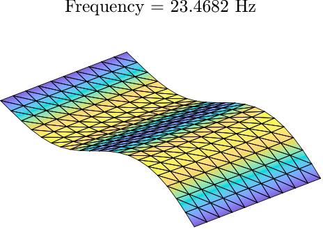
The geometrical and material properties of this curved plate are given in Table 5. The plate is simply supported at the two opposite edges aligned along the $y$ -axis in Figure 11a. The model is discretized using flat, triangular shell elements and contains 400 elements, resulting in $n=1320$ degrees of freedom. The open-source finite element code [70] directly provides us the matrices $\mathbf{M},\mathbf{C},\mathbf{K}$ and the coefficients of the nonlinearity $\mathbf{f}$ in the equations of motion (111).

Symbol	Meaning	Value [unit]
$L$	Length of plate	2 [m]
$t$	thickness of plate	10 [mm]
$H$	Width of beam	1 [m]
$E$	Young’s Modulus	70 [GPa]
$\nu$	Poisson’s ratio	0.33 [-]
$\kappa$	Viscous damping rate of material	$10^{5}$ [Pa s]
$\rho$	Density	2700 [kg/m³]

Table 5: Geometrical and material parameters of the shallow-arch structure in Figure 11a

The first mode of vibration of this structure is shown in Figure 11b and the corresponding eigenvalue pair is given by

\lambda_{1,2}=-0.29\pm 147.45\mathrm{i}.

(123)

The external forcing is again given by

\mathbf{f}^{ext}(\Omega t)=\mathbf{f}_{0}\cos(\Omega t),\quad\epsilon=0.1,

(124)

where $\mathbf{f}_{0}$ represents a vector of concentrated load in $z$ -direction with magnitude of 100 N at the mesh node located at $x=\frac{L}{2},y=\frac{H}{2}$ in Figure (11)a. We choose the forcing frequency $\Omega$ in the range 133-162 rad/s for which the eigenvalue pair $\lambda_{1,2}$ is nearly resonant with $\Omega$ (see (96)).

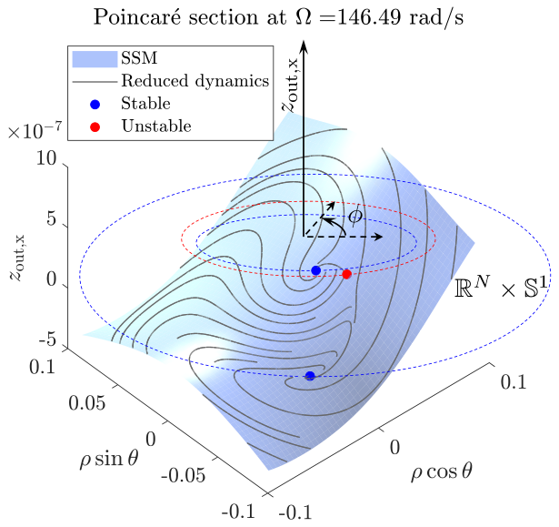
We then compute the near-resonant FRC around the first natural frequency via $\mathcal{O}(3),\mathcal{O}(5),$ and $\mathcal{O}(7)$ SSM computations using Lemma 2. Once again, Figure 12a shows the Poincaré section of the non-autonomous SSM for the near-resonant forcing frequency $\Omega=146.49$ rad/s, where we directly obtain the unstable (red) and stable (blue) periodic orbits on the FRC as hyperbolic fixed points of the reduced dynamics (89) on the SSM. The three FRCs at $\mathcal{O}(3),\mathcal{O}(5),$ and $\mathcal{O}(7)$ seem to converge to softening response shown in Figure 12b. Note that we expect a softening behavior in the FRC of shallow-arches (see, e.g., Buza et al. [64, 63]).

Due to excessive memory requirements, this FRC could not be computed using collocation approximations via coco [19] or using harmonic balance approximations via NLvib [18]. Instead, we compare this FRC to another global continuation technique based on the shooting method, which is still feasible (see Introduction).

For shooting, we use the classic Newmark time integration scheme (Newmark [71], see Géradin & Rixen [72] for a review) as the common Runge-Kutta schemes (e.g., ode45 of MATLAB) struggle to converge in structural dynamics problems. We use an open-source toolbox [46], based on the atlas-1d algorithm of coco [19] for continuation of the periodic solution trajectory obtained via shooting (see Dancowicz et al. [14]). We use a constant time step throughout time integration which is chosen by dividing the time span $T=\frac{2\pi}{\Omega}$ into 100 equal intervals. We found this choice of time step to be nearly optimal for this problem as larger time steps lead to non-quadratic convergence during Newton-Raphson iterations and smaller time steps result in slower computations. The stability of the response is computed by integrating the equations of variation around the converged periodic orbit.

$n$	Computation time [hours:minutes:seconds]
(number of degrees	Shooting method	SSM $\mathcal{O}(3)$	SSM $\mathcal{O}(5)$	SSM $\mathcal{O}(7)$
of freedom)	(Newmark)	(SSMTool 2.0 [69])
1,320	52:50:14	00:00:07	00:00:12	00:00:28

Table 6: Computation time for obtaining the FRCs depicted in Figure 12. All computations were performed on MATLAB version 2019b installed on a Windows-PC with Intel Core i7-4790 CPU @ 3.60GHz and 32 GB RAM.

The total time consumed in model generation and coefficient assembly was 33 seconds on a Windows-PC with Intel Core i7-4790 CPU @ 3.60GHz and 32 GB RAM. This includes the time spent in computing the first 10 eigenvalues of this system, which took less than 1 second. Figure 12b shows that this shooting based global continuation agrees with the SSM-based approximation to the FRC. Obtaining this FRC via the shooting methods, however, takes more than 2 days, in contrast to SSM-based approximation using the proposed computational methodology, which still takes less than a minute even at $\mathcal{O}(7)$ , as shown in Table 6.

6.4 Aircraft Wing

As a final example, we consider the finite element model of a geometrically nonlinear aircraft wing originally presented by Jain et al [65] (see Figure 13). The wing is cantilevered at one of its ends and the structure is meshed using flat triangular shell elements featuring 6 degrees of freedom per node. With 49,968 elements and 133,920 degrees of freedom, this model provides a physically relevant as well as computationally realistic problem that is beyond feasibility for global continuation techniques based on collocation, spectral and shooting methods, as shown by previous examples. The open-source finite element code [70] directly provides us the matrices $\mathbf{M},\mathbf{K}$ and the coefficients of the nonlinearity $\mathbf{f}$ in the equations of motion (111).

Symbol	Meaning	Value [unit]
$L$	Length of wing ( $z$ direction)	5 [m]
$H$	Height of wing ( $y$ direction)	0.1 [m]
$W$	Width of wing ( $x$ direction)	0.9 [m]
$t$	thickness of elements	1.5 [mm]
$E$	Young’s Modulus	70 [GPa]
$\nu$	Poisson’s ratio	0.33 [-]
$\rho$	Density	2700 [kg/m³]

Table 7: Geometrical and material parameters of the shallow-arch structure in Figure 11a

For assembling coefficients on a problem of this size, we used the Euler supercomputering cluster at ETH Zurich. The total time consumed in model generation and coefficient assembly was 1 hour 21 minutes and 38 seconds without any parallelization. This time includes the time taken for computing the first 10 eigenvalues of this system, which was approximately 5 seconds. The main bottleneck was the memory consumption during the assembly of the coefficients of the nonlinearity $\mathbf{f}$ , where the peak memory consumption was around $183$ GB. However, once assembled, these coefficients consume only about 1.8 GB of RAM. This extraordinary memory consumption during assembly occurs due to a sub-optimal assembly procedure of sparse tensors [66]. To avoid these bottlenecks, parallel computing and distributed memory architectures need to be employed, which are currently not available in the packages we have used.

In this example, we choose Rayleigh damping (see, e.g., Géradin & Rixen [72]), which is commonly employed in structural dynamics applications to construct the damping matrix $\mathbf{C}=\alpha\mathbf{M}+\beta\mathbf{K}$ as a linear combination of mass and stiffness matrices. The constants $\alpha,\beta$ are chosen to ensure a damping ratio of 0.4% along the first two vibration modes. The eigenvalue pair associated to the first mode of vibration is given by

\lambda_{1,2}=-0.0587\pm 29.3428\mathrm{i}.

(125)

Once again, we choose harmonic external forcing given by

\mathbf{f}^{ext}(\Omega t)=\mathbf{f}_{0}\cos(\Omega t),\quad\epsilon=0.01,

(126)

where $\mathbf{f}_{0}$ represents a vector of concentrated loads at the tip nodes 1 and 2 (see Figure (13)b) in the transverse $y$ -direction each with a magnitude of 100 N. We choose the forcing frequency $\Omega$ in the range 26.4-32.3 rad/s for which the eigenvalue pair $\lambda_{1,2}$ is nearly resonant with $\Omega$ (see (96)). We then compute the near-resonant FRCs around the first natural frequency via $\mathcal{O}(3),\mathcal{O}(5),$ and $\mathcal{O}(7)$ SSM computations using Lemma 2.

Similarly to the previous examples, Figure 14a shows the Poincaré section of the non-autonomous SSM for the near-resonant forcing frequency $\Omega=29.8$ rad/s. The hyperbolic fixed points of the reduced dynamics (2) on the SSM directly provide the stable (blue) and unstable (red) periodic orbits on the FRC for different values of forcing frequency $\Omega$ . On a macro-level, this wing example resembles a cantilevered beam and we expect a hardening type response. Indeed, the three FRCs at $\mathcal{O}(3),\mathcal{O}(5),$ and $\mathcal{O}(7)$ converge towards a hardening-type response, as shown in Figure 14b.

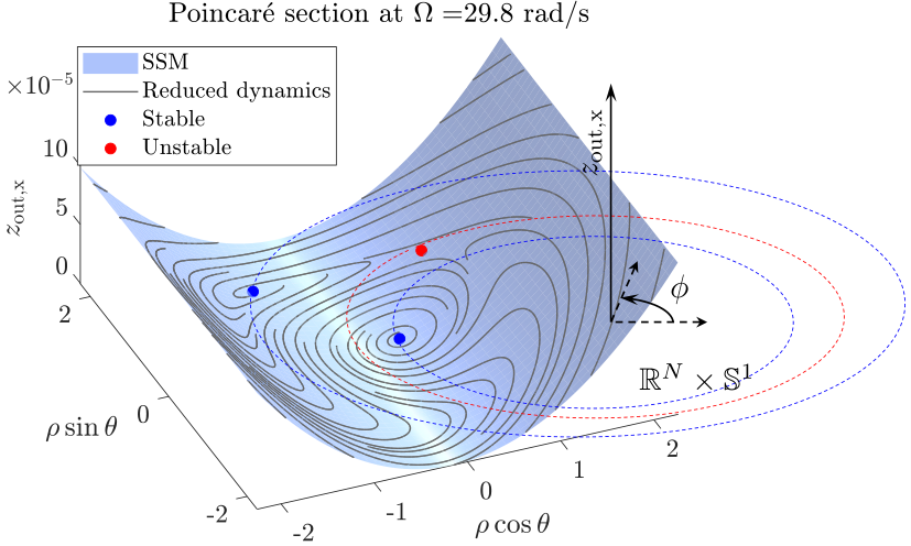
Table 8 depicts the computational resources consumed in obtaining these three FRCs. The peaks in memory consumption reported in Table 8 occur during the composition of nonlinearity (see eq. (27)). Note that these peaks are short-lived, however, as the average memory consumption during all these computations are much lower. We remark that in the context of finite-element applications, these memory peaks can be significantly reduced by implementing the nonlinearity composition at the element-level in contrast to the currently performed implementation at the full system level. Once again, use of parallel computing and distributed memory architectures would be greatly beneficial in this context.

SSM order	Computation time [hours:minutes:seconds]	Peak memory consumption	Average memory consumption
SSM- $\mathcal{O}(3)$	00:11:17	$\approx$ 24 GB	$\approx$ 9 GB
SSM- $\mathcal{O}(5)$	00:35:47	$\approx$ 33 GB	$\approx$ 10 GB
SSM- $\mathcal{O}(7)$	01:47:51	$\approx$ 88 GB	$\approx$ 19 GB

Table 8: Computation time and memory requirements for obtaining the three FRCs depicted in Figure 14. All computations were performed on MATLAB version 2019b installed on the ETH Zürich Euler supercomputing cluster on a single node with

100,000

MB (

\approx 100

GB) of RAM.

7 Conclusions

In this work, we have reformulated the parametrization method for local approximations of invariant manifolds and their reduced dynamics in the context of high-dimensional nonlinear mechanics problems. In this class of problems, the classically used system diagonalization at the linear level is no longer feasible. Instead, we have developed expressions that enable the computation of invariant manifolds and their reduced dynamics in physical coordinates using only the master modes associated with the invariant manifold. Hence, these computations facilitate mathematically rigorous nonlinear model reduction in very high-dimensional problems. A numerical implementation of the proposed computational methodology is available in the open-source MATLAB package, SSMTool 2.0 [69], which enables the computation of invariant manifolds in finite element-based discretized problems via an integrated finite element solver [70] and bifurcation analysis of the reduced dynamics on these invariant manifolds via its coco [19] integration.

We have connected this computational methodology to several applications of engineering significance, including the computation of parameter-dependent center manifolds; Lyapunov subcenter manifolds (LSM) and their associated conservative backbone curves; and Spectral Submanifolds (SSM) and their associated forced response curves (FRCs) in dissipative mechanical systems. We have also demonstrated fast and reliable computations of FRCs via a normal form style parametrization of SSMs in very large mechanical structures, which has been a computationally intractable task for other available approaches.

While our examples focused on the applications of two-dimensional SSMs, this automated computation procedure and its numerical implementation [69] can treat higher-dimensional invariant manifolds as well. Specifically, the reduced dynamics on higher-dimensional SSMs can be used for the direct computation of FRCs in internally-resonant mechanical systems featuring energy transfer among multiple modes, as will be demonstrated in forthcoming publications (Li et al. [73], Li & Haller [74]). Furthermore, in the non-autonomous setting, we have restricted our expressions to the leading-order contributions from the forcing. Similar expressions, however, can also be obtained for higher-order terms at the non-autonomous level, which is relevant for the nonlinear analysis of parametrically excited systems. These expressions and the related numerical implementation are currently under development.

Finally, as we have noted, these computations will further benefit from parallelization since the invariance equations can be solved independently for each monomial/Fourier multi-index (see Remarks 2 and 4, and Section 6.4). This development is currently underway and will be reported elsewhere.

Acknowledgements

We are thankful to Mingwu Li for help in using coco, for his careful proof-reading of this manuscript and for providing valuable comments. We also thank Harry Dankowicz for helpful suggestions and pointing us to the atlas- $k$ d algorithm in coco.

Conflicts of interest

The authors declare that they have no conflict of interest.

Funding

No specific funding was received for this work.

Data availability

The numerical implementation of algorithms and results discussed in this work are available in the form of an open-source MATLAB software at the following DOI: http://doi.org/10.5281/zenodo.4614202

Appendix A Basic propositions

Proposition 1.

Let $\mathbf{Q}\in\mathbb{C}^{M\times M}$ be any semisimple matrix with eigenvalues $\mu_{1},\dots,\mu_{M}$ (including repetitions) and corresponding left and right eigenvectors $\mathbf{p}_{1},\dots,\mathbf{p}_{M}\in\mathbb{C}^{M}$ and $\mathbf{r}_{1},\dots,\mathbf{r}_{M}\in\mathbb{C}^{M}$ . Then, for any $i\in\mathbb{N}$ , the matrix

\boldsymbol{\mathcal{Q}}_{i}:=\text{$\sum_{j=1}^{i}$$\left(\mathbf{I}_{M}\right)^{\otimes j-1}\otimes\mathbf{Q}\otimes\left(\mathbf{I}_{M}\right)^{\otimes i-j}$}\in\mathbb{C}^{M^{i}\times M^{i}}

(127)

is semisimple and its eigenvalues are

\mu_{\mathbf{\boldsymbol{\ell}}}=\mu_{\ell_{1}}+\dots+\mu_{\ell_{i}},\quad\boldsymbol{\ell}\in\Delta_{i,M}

(128)

with the left and right eigenvectors corresponding to any eigenvalue $\mu_{\mathbf{\boldsymbol{\ell}}}$ explicitly given as $\mathbf{p}_{\boldsymbol{\ell}}:=\mathbf{p}_{\ell_{1}}\otimes\dots\otimes\mathbf{p}_{\ell_{i}}$ and $\mathbf{q}_{\boldsymbol{\ell}}:=\mathbf{q}_{\ell_{1}}\otimes\dots\otimes\mathbf{q}_{\ell_{i}}.$

Proof.

The proof involves a straight-forward verification of the statement. The eigenvalues and the left and right eigenvectors of $\mathbf{Q}$ satisfy

	$\displaystyle\mathbf{Qp}_{j}$	$\displaystyle=\mu_{j}\mathbf{p}_{j},\quad j=1,\dots,M,$		(129)
	$\displaystyle\mathbf{q}_{j}^{\star}\mathbf{Q}$	$\displaystyle=\mu_{j}\mathbf{q}_{j}^{\star},\quad j=1,\dots,M,$		(130)

We first verify that $\mu_{\mathbf{\boldsymbol{\ell}}}$ (see eq. (128)) is an eigenvalue of $\boldsymbol{\mathcal{Q}}_{i}$ (see eq. (127)) with eigenvector $\mathbf{p}_{\boldsymbol{\ell}}:=\left(\mathbf{p}_{\ell_{1}}\otimes\dots\otimes\mathbf{p}_{\ell_{i}}\right)$ , i.e.,

	$\displaystyle\boldsymbol{\mathcal{Q}}_{i}\mathbf{p}_{\boldsymbol{\ell}}$	$\displaystyle=\left[\sum_{j=1}^{i}\underbrace{\mathbf{I}_{m}\otimes\dots\otimes\overset{\overset{j-\mathrm{th\,position}}{\uparrow}}{\mathbf{Q}}\otimes\dots\otimes\mathbf{I}_{m}}_{i-\mathrm{terms}}\right]\left[\mathbf{p}_{\ell_{1}}\otimes\dots\otimes\mathbf{p}_{\ell_{i}}\right]$
		$\displaystyle=\sum_{j=1}^{i}\mathbf{p}_{\ell_{1}}\otimes\dots\otimes\mathbf{Q}\mathbf{p}_{\ell_{j}}\otimes\dots\otimes\mathbf{p}_{\ell_{i}}$
		$\displaystyle=\sum_{j=1}^{i}\mathbf{p}_{\ell_{1}}\otimes\dots\otimes\mu_{\ell_{j}}\mathbf{p}_{\ell_{j}}\otimes\dots\otimes\mathbf{p}_{\ell_{i}}$
		$\displaystyle=\sum_{j=1}^{i}\mu_{\ell_{j}}\left(\mathbf{p}_{\ell_{1}}\otimes\dots\otimes\mathbf{p}_{\ell_{i}}\right)$
		$\displaystyle=\mu_{\mathbf{\boldsymbol{\ell}}}\mathbf{p}_{\boldsymbol{\ell}},$

where we have used basic properties of the Kronecker product (see, e.g., Van Loan [53]) along with with eq. (130). Similarly, using eq. (129), we can verify that the left eigenvector corresponding to the eigenvalue $\mu_{\mathbf{\boldsymbol{\ell}}}$ is given by $\mathbf{q}_{\boldsymbol{\ell}}:=\mathbf{q}_{\ell_{1}}\otimes\dots\otimes\mathbf{q}_{\ell_{i}}$ , i.e.,

\mathbf{q}_{\boldsymbol{\ell}}^{\star}\boldsymbol{\mathcal{Q}}_{i}=\mu_{\mathbf{\boldsymbol{\ell}}}\mathbf{q}_{\boldsymbol{\ell}}^{\star}.

We note that since $\mathbf{p}_{1},\dots,\mathbf{p}_{M}$ are linearly independent since $\mathbf{Q}$ is semisimple. Then, using the fact that for any two linearly independent vectors $\mathbf{a}$ and $\mathbf{b}$ , the vectors $\mathbf{a}\otimes\mathbf{b}$ and $\mathbf{b}\otimes\mathbf{a}$ are also linearly independent, we conclude that all $M^{i}$ eigenvectors $\mathbf{p}_{\boldsymbol{\ell}}$ with $\boldsymbol{\ell}\in\Delta_{i}$ of $\boldsymbol{\mathcal{Q}}_{i}$ are linearly independent. Hence, $\boldsymbol{\mathcal{Q}}_{i}$ is semi-simple. ∎

Proposition 2.

Let $\mathbf{\lambda}\in\mathbb{\mathbb{C}}$ be a generalized eigenvalue of a matrix pair $\mathbf{A},\mathbf{B}\in\mathbb{C}^{N\times N}$ with the corresponding left and right eigenvectors $\mathbf{u},\mathbf{v}\in\mathbb{C}^{N}$ , and $\mu\in\mathbb{C}$ be a generalized eigenvalue of a matrix pair $\mathbf{C},\mathbf{D}\in\mathbb{C}^{M\times M}$ with the corresponding left and right eigenvectors $\mathbf{e},\mathbf{f}\in\mathbb{C}^{M}$ for any $M,N\in\mathbb{N}$ . Then $\lambda\mu$ is a generalized eigenvalue for the matrix pair $\left(\mathbf{C}\otimes\mathbf{A}\right),\left(\mathbf{D}\otimes\mathbf{B}\right)\in\mathbb{C}^{NM\times NM}$ with the corresponding left and right eigenvectors $(\mathbf{e}\otimes\mathbf{u}),(\mathbf{f}\otimes\mathbf{v})\in\mathbb{C}^{MN}$ . Furthermore, if $\lambda\mu=1$ , then the matrix

\mathbf{E}:=\mathbf{D}\otimes\mathbf{B}-\mathbf{C}\otimes\mathbf{A}\in\mathbb{C}^{NM\times NM}

(131)

is singular with $(\mathbf{e}\otimes\mathbf{u})\in\ker\left(\mathbf{E}^{\star}\right)$ and $(\mathbf{f}\otimes\mathbf{v})\in\ker\left(\mathbf{E}\right)$ .

Proof.

Since $\lambda$ is a generalized eigenvalue of the matrix pair $\mathbf{A},\mathbf{B}$ with $\mathbf{w},\mathbf{v}$ being the corresponding left and right eigenvectors, we have

	$\displaystyle\mathbf{Av}$	$\displaystyle=\lambda\mathbf{Bv},$		(132)
	$\displaystyle\mathbf{u^{\star}}\mathbf{A}$	$\displaystyle=\lambda\mathbf{u^{\star}}\mathbf{B}.$		(133)

Similarly, for the matrix pair $\mathbf{C},\mathbf{D}$ with eigenvalue $\mu$ and $\mathbf{e},\mathbf{f}$ being the corresponding left and right eigenvectors, we have

	$\displaystyle\mathbf{Cf}$	$\displaystyle=\mu\mathbf{D}\mathbf{f},$		(134)
	$\displaystyle\mathbf{e^{\star}}\mathbf{C}$	$\displaystyle=\mu\mathbf{e^{\star}}\mathbf{D}.$		(135)

We verify that $\lambda\mu$ is a generalized eigenvalue of the matrix pair $\left(\mathbf{C}\otimes\mathbf{A}\right),\left(\mathbf{D}\otimes\mathbf{B}\right)$ with eigenvector $(\mathbf{f}\otimes\mathbf{v})$ , i.e.,

$\displaystyle\left(\mathbf{C}\otimes\mathbf{A}\right)(\mathbf{f}\otimes\mathbf{v})$	$\displaystyle=\left(\mathbf{C}\mathbf{f}\right)\otimes\left(\mathbf{A}\mathbf{v}\right)$
	$\displaystyle=\left(\mu\mathbf{D}\mathbf{f}\right)\otimes\left(\lambda\mathbf{Bv}\right)$
	$\displaystyle=\lambda\mu\left(\mathbf{D}\mathbf{f}\right)\otimes\left(\mathbf{Bv}\right)$
	$\displaystyle=\lambda\mu\left(\mathbf{D}\otimes\mathbf{B}\right)(\mathbf{f}\otimes\mathbf{v}),$	(136)

where we have used eqs. (132), (134) along with basic properties of the Kronecker product of matrices (see, e.g., Van Loan [53]). Similarly, using eqs. (133), (135), we can show that

(\mathbf{e}\otimes\mathbf{u})^{\star}\left(\mathbf{C}\otimes\mathbf{A}\right)=\lambda\mu(\mathbf{e}\otimes\mathbf{u})^{\star}\left(\mathbf{D}\otimes\mathbf{B}\right),

(137)

which proves that $(\mathbf{e}\otimes\mathbf{u})$ is the generalized left-eigenvector for the generalized eigenvalue $\lambda$ for the generalize first part of the proposition.

Finally, substituting $\lambda\mu=1$ in eqs. (136), (136), we obtain

	$\displaystyle\left[\left(\mathbf{C}\otimes\mathbf{A}\right)-\left(\mathbf{D}\otimes\mathbf{B}\right)\right](\mathbf{f}\otimes\mathbf{v})$	$\displaystyle=\mathbf{0},$
	$\displaystyle(\mathbf{e}\otimes\mathbf{u})^{\star}\left[\left(\mathbf{C}\otimes\mathbf{A}\right)-\left(\mathbf{D}\otimes\mathbf{B}\right)\right]$	$\displaystyle=\mathbf{0},$

which proves that the matrix $\mathbf{E}$ (see definition (131)) is singular and the vectors $(\mathbf{f}\otimes\mathbf{v})$ and $(\mathbf{e}\otimes\mathbf{u})$ belong to its left and right kernels. ∎

Appendix B Proof of Lemma 1

In polar coordinates $\mathbf{p}=\mathbf{P}(\rho,\theta):=\rho\left[\begin{array}[]{c}e^{\mathrm{i}\theta}\\ e^{-\mathrm{i}\theta}\end{array}\right]$ , the reduced dynamics (78) is given as

\left[\begin{array}[]{c}\dot{\rho}\\ \dot{\theta}\end{array}\right]=\left[\begin{array}[]{c}a(\rho)\\ \omega(\rho)\end{array}\right]=\left[\begin{array}[]{c}0\\ \omega_{m}\end{array}\right]+\sum_{\ell\in\mathbb{N}}\left[\begin{array}[]{c}\mathrm{Re}(\gamma_{\ell})\rho^{2\ell+1}\\ \mathrm{Im}(\gamma_{\ell})\rho^{2\ell}\end{array}\right].

(138)

Now, since the equation for $\dot{\rho}$ is a scalar ODE decoupled from the phase $\theta$ , the only possible steady states are fixed points $\dot{\rho}=0$ , i.e., $\rho=\rho(0)=$ constant. Therefore, $\dot{\theta}=\omega(\rho)$ represents a constant angular frequency depending on the constant steady-state amplitude $\rho$ . Since the LSM is an analytic manifold, the function $a,\omega$ describing reduced dynamics on the LSM are also analytic. Note that since the LSM is filled with periodic orbits in an open neighborhood of the origin, $a(\rho)$ must be identically zero because any non-trivial polynomial expression for $a$ would result in isolated periodic orbits on the LSM. Thus, we deduce that our computational procedure must result in

\mathrm{Re}(\gamma_{\ell})=0\quad\forall\ell\in\mathbb{N}.

Finally, as the LSM is foliated with periodic orbits in an open neighborhood of the origin, the equation $\dot{\theta}=\omega(\rho)$ expresses the frequency of oscillation as a function any given constant amplitude $\rho$ for the periodic orbits on the LSM. Hence the conservative backbone around the $m^{\mathrm{th}}$ mode is given by the relation (79).

Appendix C Proof of Lemma 2

Using polar coordinates $\mathbf{p}=\mathbf{P}(\rho,\theta):=\rho\left[\begin{array}[]{c}e^{\mathrm{i}\theta}\\ e^{-\mathrm{i}\theta}\end{array}\right]$ , we rewrite the first equation in the system (98) as

\dot{p}_{1}=\dot{\rho}e^{\mathrm{i}\theta}+\mathrm{i}\dot{\theta}\rho e^{\mathrm{i}\theta}=\lambda\rho e^{\mathrm{i}\theta}+\sum_{\ell\in\mathbb{N}}\gamma_{\ell}\rho^{2\ell+1}e^{\mathrm{i}\theta}+fe^{\mathrm{i}\eta\phi},

(139)

where

f:=\epsilon\mathbf{u}_{j}^{\star}\mathbf{F}_{\eta}^{ext}.

Dividing eq. (139) by $e^{\mathrm{i}\theta}$ and introducing the phase shift $\psi=\theta-\eta\phi$ , we obtain

\dot{\rho}+\mathrm{i}\left(\dot{\psi}+\eta\Omega\right)\rho=\lambda\rho+\sum_{\ell\in\mathbb{N}}\gamma_{\ell}\rho^{2\ell+1}+\epsilon fe^{-\mathrm{i}\psi}.

(140)

Comparing the real and imaginary parts in eq. (140), we obtain the polar reduced dynamics given in eq. (2), which concludes the proof of (i).

The fixed points of system (2) are obtained by equating its right-hand-side to zero as

\mathbf{r}(\rho,\psi,\Omega)=\mathbf{0}.

(141)

Any such fixed point represent a periodic orbit for the reduced system (2) with constant polar radius $\rho$ and constant phase difference $\psi$ with respect to the cyclic variable $\eta\phi$ , which has the angular frequency $\eta\Omega$ . Hence, we obtain a 1-dimensional submanifold of zeros upon solving (141), whose projection in the $(\rho,\Omega)$ provides us the FRC. Eliminating $\psi$ from eq. (141), we obtain the fixed points as the set of points $\left(\rho,\Omega\right)$ that satisfy the equation

\left[a(\rho)\right]^{2}+\left[b(\rho,\Omega)\right]^{2}=|f|^{2},

(142)

which proves statement (ii).

Solving the two equations (141) for $\cos\psi$ and $\sin\psi$ , we obtain

	$\displaystyle\cos\psi$	$\displaystyle=-\frac{\left(a(\rho)\mathrm{Re}(f)+b(\rho,\Omega)\mathrm{Im}(f)\right)}{\|f\|^{2}},$
	$\displaystyle\sin\psi$	$\displaystyle=\frac{\left(b(\rho,\Omega)\mathrm{Re}(f)-a(\rho)\mathrm{Im}(f)\right)}{\|f\|^{2}},$

which provides the phase shift as

\psi=\arctan\left(\frac{b(\rho,\Omega)\mathrm{Re}(f)-a(\rho)\mathrm{Im}(f)}{-a(\rho)\mathrm{Re}(f)-b(\rho,\Omega)\mathrm{Im}(f)}\right),

and hence proves statement (iii).

Finally, we rewrite the reduced dynamics (2) in its standard form as

\left[\begin{array}[]{c}\dot{\rho}\\ \dot{\psi}\end{array}\right]=\left[\begin{array}[]{c}a(\rho)\\ \frac{b(\rho,\Omega)}{\rho}\end{array}\right]+\left[\begin{array}[]{cc}1&0\\ 0&\frac{1}{\rho}\end{array}\right]\left[\begin{array}[]{cc}\cos\psi&\sin\psi\\ -\sin\psi&\cos\psi\end{array}\right]\left[\begin{array}[]{c}\mathrm{Re}\left(f\right)\\ \mathrm{Im}\left(f\right)\end{array}\right].

(143)

The Jacobian of the right-hand side of eq. (143) evaluated at the fixed point $(\rho,\psi)$ is given by (110) and its eigenvalues can be used to conclude the stability of any hyperbolic fixed point via linearized stability analysis, which proves statement (iv).

References

[1] Guckenheimer, J., & Holmes, P. (1983). Nonlinear Oscillations, Dynamical Systems, and Bifurcations of Vector Fields. https://doi.org/10.1007/978-1-4612-1140-2
[2] Fenichel, N. (1971). Persistence and Smoothness of Invariant Manifolds for Flows. Indiana University Mathematics Journal, 21(3), 193–226. https://doi.org/10.1512/iumj.1971.21.21017
[3] Fenichel, N. (1974). Asymptotic Stability with Rate Conditions. Indiana University Mathematics Journal, 23(12), 1109–1137. https://doi.org/10.1512/iumj.1974.23.23090
[4] Fenichel, N. (1977). Asymptotic Stability with Rate Conditions, II. Indiana University Mathematics Journal, 26(1), 81–93. https://doi.org/10.1512/iumj.1977.26.26006
[5] Hirsch, M. W., Pugh, C. C., & Shub, M. (1977). Invariant Manifolds. https://doi.org/10.1007/BFb0092042
[6] Wiggins, S. (1994). Normally Hyperbolic Invariant Manifolds in Dynamical Systems. https://doi.org/10.1007/978-1-4612-4312-0
[7] Eldering, J. (2013). Normally Hyperbolic Invariant Manifolds: The Noncompact Case. Atlantis Press. https://doi.org/10.2991/978-94-6239-003-4
[8] Nipp, K., & Stoffer, D. (2013). Invariant Manifolds in Discrete and Continuous Dynamical Systems. https://doi.org/10.4171/124
[9] Krauskopf, B., & Osinga, H. M. (2003). Computing geodesic level sets on global (un)stable manifolds of vector fields. SIAM Journal on Applied Dynamical Systems, 2(4), 546–569. https://doi.org/10.1137/030600180
[10] Krauskopf, B., Osinga, H. M., Doedel, E. J., Henderson, M. E., Guckenheimer, J., Vladimirsky, A., Dellnitz, M., Junge, O. (2005). A survey of methods for computing (UN)stable manifolds of vector fields. International Journal of Bifurcation and Chaos, 15, 763–791. https://doi.org/10.1142/S0218127405012533
[11] B. Krauskopf, H.M. Osinga, and J. Galán-Vioque (Eds.), Numerical Continuation Methods for Dynamical Systems, Canopus Publishing Ltd., Bristol, UK, 2007.
[12] Keller, H. B. (1968). Numerical Methods for Two-Point Boundary-Value Problems. Blaisdell Publishing Company, Waltham, Massachusetts.
[13] Stoer, J., & Bulirsch, R. (2002). Introduction to Numerical Analysis. Springer, New York. https://doi.org/10.1007/978-0-387-21738-3
[14] Dankowicz, H., Wang, Y., Schilder, F., & Henderson, M. E. (2020). Multidimensional manifold continuation for adaptive boundary-value problems. Journal of Computational and Nonlinear Dynamics, 15(5). https://doi.org/10.1115/1.4046498
[15] Carraro, T., Geiger, M., Körkel, S., & Rannacher, R. (Eds.). (2015). Multiple Shooting and Time Domain Decomposition Methods. https://doi.org/10.1007/978-3-319-23321-5
[16] Doedel, E., Oldeman, B.: Auto-07p: Continuation and Bifurcation Software for ordinary differential equations, url: http://indy.cs.concordia.ca/auto/
[17] Dhooge, A., Govaerts, W., Kuznetsov, Y. (2003) Matcont: a MATLAB package for numerical bifurcation analysis of odes. ACM Trans. Math. softw. 29(2), 141–164.
[18] Krack, M., & Gross, J. (2019). Harmonic Balance for Nonlinear Vibration Problems. Cham: Springer International Publishing. https://doi.org/10.1007/978-3-030-14023-6
[19] Dankowicz, H., & Schilder, F. (2013). Recipes for Continuation.Society for Industrial and Applied Mathematics, Philadelphia. https://doi.org/10.1137/1.9781611972573
[20] Stewart, G. W. (2002). A Krylov-Schur algorithm for large eigenproblems. SIAM Journal on Matrix Analysis and Applications, 23(3), 601–614. https://doi.org/10.1137/S0895479800371529
[21] Lehoucq, R. B., Sorensen, D. C., & Yang, C. (1998). ARPACK Users’ Guide: Solution of Large-Scale Eigenvalue Problems with Implicitly Restarted Arnoldi Methods. https://doi.org/10.1137/1.9780898719628
[22] Golub, G. H., & Van Der Vorst, H. A. (2000). Eigenvalue computation in the 20th century. Journal of Computational and Applied Mathematics, 123(1–2), 35–65. https://doi.org/10.1016/S0377-0427(00)00413-1
[23] Engelborghs, K., Luzyanina, T., Samaey, G. (2001) DDE-BIFTOOL v. 2.00: a Matlab package for bifurcation analysis of delay differential equations, Technical Report TW-330, Department of Computer Science, K.U.Leuven, Leuven, Belgium.
[24] Szalai, R. (2013) Knut: a continuation and bifurcation software for delay-differential equations. https://github.com/rs1909/knut.git
[25] C. Simó, (1990) On the Analytical and Numerical Approximation of Invariant Manifolds, Modern Methods in Celestial Mechanics, Comptes Rendus de la 13ieme Ecole Printemps d’Astrophysique de Goutelas (France), 24–29 Avril, 1989. Edited by Daniel Benest and Claude Froeschlé. Gif-sur-Yvette: Editions Frontieres, 285–330.
[26] Fuming, M., & Küpper, T. (1994). Numerical calculation of invariant manifolds for maps. Numerical Linear Algebra with Applications, 1(2), 141–150. https://doi.org/10.1002/nla.1680010205
[27] Cabré, X., Fontich, E., & de la Llave, R. (2003). The parameterization method for invariant manifolds I: Manifolds associated to non-resonant subspaces. Indiana University Mathematics Journal, 52(2), 283–328. https://doi.org/10.1512/iumj.2003.52.2245
[28] Cabré, X., Fontich, E., & de la Llave, R. (2003). The parameterization method for invariant manifolds II: regularity with respect to parameters. Indiana University Mathematics Journal, 52(2), 329–360. https://doi.org/10.1512/iumj.2003.52.2407
[29] Cabré, X., Fontich, E., & de la Llave, R. (2005). The parameterization method for invariant manifolds III: overview and applications. Journal of Differential Equations, 218(2), 444–515. https://doi.org/10.1016/j.jde.2004.12.003
[30] Haro, A., & de la Llave, R. (2006). A parameterization method for the computation of invariant tori and their whiskers in quasi-periodic maps: Rigorous results. Journal of Differential Equations, 228(2), 530–579. https://doi.org/10.1016/j.jde.2005.10.005
[31] Haro, A., & De La Llave, R. (2007). A parameterization method for the computation of invariant tori and their whiskers in quasi-periodic maps: Explorations and mechanisms for the breakdown of hyperbolicity. SIAM Journal on Applied Dynamical Systems, 6(1), 142–207. https://doi.org/10.1137/050637327
[32] Haro, A., & De La Llave, R. (2006). A parameterization method for the computation of invariant tori and their whiskers in quasi-periodic maps: Numerical algorithms. Discrete and Continuous Dynamical Systems - Series B, 6(6), 1261–1300. https://doi.org/10.3934/dcdsb.2006.6.1261
[33] Haro, A., Canadell, M., Figueras, J.-L., Luque, A., & Mondelo, J. M. (2016). The Parameterization Method for Invariant Manifolds. https://doi.org/10.1007/978-3-319-29662-3
[34] Mireles James, J. D. (2015). Polynomial approximation of one parameter families of (un)stable manifolds with rigorous computer assisted error bounds. Indagationes Mathematicae, 26(1), 225–265. https://doi.org/10.1016/j.indag.2014.10.002
[35] Castelli, R., Lessard, J. P., & James, J. D. M. (2015). Parameterization of Invariant Manifolds for Periodic Orbits I: Efficient Numerics via the Floquet Normal Form. SIAM Journal on Applied Dynamical Systems, 14(1), 132–167. https://doi.org/10.1137/140960207
[36] Tisseur, F., & Meerbergen, K. (2001). The quadratic eigenvalue problem. SIAM Review, 43(2), 235–286. https://doi.org/10.1137/S0036144500381988
[37] Ponsioen, S., Pedergnana, T., & Haller, G. (2018). Automated computation of autonomous spectral submanifolds for nonlinear modal analysis. Journal of Sound and Vibration, 420, 269–295. https://doi.org/10.1016/J.JSV.2018.01.048
[38] T. Breunung & G. Haller, Explicit backbone curves from spectral submanifolds of forced-damped nonlinear mechanical systems. Proc. R. Soc. A 474 (2018) 20180083.
[39] Veraszto, Z., Ponsioen, S., & Haller, G. (2020). Explicit third-order model reduction formulas for general nonlinear mechanical systems. Journal of Sound and Vibration, 468, 115039. https://doi.org/10.1016/j.jsv.2019.115039
[40] Szalai, R., Ehrhardt, D., & Haller, G. (2017). Nonlinear model identification and spectral submanifolds for multi-degree-of-freedom mechanical vibrations. Proceedings of the Royal Society A: Mathematical, Physical and Engineering Science, 473(2202), 20160759. https://doi.org/10.1098/rspa.2016.0759
[41] Ponsioen, S., Pedergnana, T., & Haller, G. (2019). Analytic prediction of isolated forced response curves from spectral submanifolds. Nonlinear Dynamics, 98(4), 2755–2773. https://doi.org/10.1007/s11071-019-05023-4
[42] Ponsioen, S., Jain, S., & Haller, G. (2020). Model reduction to spectral submanifolds and forced-response calculation in high-dimensional mechanical systems. Journal of Sound and Vibration, 488, 115640. https://doi.org/10.1016/j.jsv.2020.115640
[43] Vizzaccaro, A., Shen, Y., Salles, L., Blahoš, J., & Touzé, C. (2021). Direct computation of nonlinear mapping via normal form for reduced-order models of finite element nonlinear structures. Computer Methods in Applied Mechanics and Engineering, 384, 113957. https://doi.org/10.1016/j.cma.2021.113957
[44] Opreni, A., Vizzaccaro, A., Frangi, A., & Touzé, C. (2021). Model order reduction based on direct normal form: application to large finite element MEMS structures featuring internal resonance. Nonlinear Dynamics 2021, 105(2), 1237–1272. https://doi.org/10.1007/S11071-021-06641-7
[45] Touzé, C., Vizzaccaro, A., & Thomas, O. (2021). Model order reduction methods for geometrically nonlinear structures: a review of nonlinear techniques. Nonlinear Dynamics, 105(2), 1141–1190. https://doi.org/10.1007/s11071-021-06693-9
[46] Li, M. and Dankowicz, H. (2021). A COCO-based shooting toolbox for dynamical systems. https://github.com/mingwu-li/forward
[47] Kelley, A. (1969). Analytic two-dimensional subcenter manifolds for systems with an integral. Pacific Journal of Mathematics, 29(2), 335–350. https://doi.org/10.2140/pjm.1969.29.335
[48] Jain, S., Tiso, P., & Haller, G. (2018). Exact nonlinear model reduction for a von Kármán beam: slow-fast decomposition and spectral submanifolds. Journal of Sound and Vibration, 423, 195–211. https://doi.org/10.1016/J.JSV.2018.01.049
[49] Guckenheimer, J., Krauskopf, B., Osinga, H. M., & Sandstede, B. (2015). Invariant manifolds and global bifurcations. Chaos, 25(9), 097604. https://doi.org/10.1063/1.4915528
[50] Murdock, J. (2003). Normal Forms and Unfoldings for Local Dynamical Systems. New York, NY: Springer New York. https://doi.org/10.1007/b97515
[51] Golub, G. H., & van Loan, C. F. (2013). Matrix Computations. Retrieved from https://jhupbooks.press.jhu.edu/title/matrix-computations
[52] Haller, G., & Ponsioen, S. (2016). Nonlinear normal modes and spectral submanifolds: existence, uniqueness and use in model reduction. Nonlinear Dynamics, 86(3), 1493–1534. https://doi.org/10.1007/s11071-016-2974-z
[53] Loan, C. F. V. (2000). The ubiquitous Kronecker product. Journal of Computational and Applied Mathematics, 123(1–2), 85–100. https://doi.org/10.1016/S0377-0427(00)00393-9
[54] Kuznetsov, Y. A. (2004). Elements of Applied Bifurcation Theory. https://doi.org/10.1007/978-1-4757-3978-7
[55] Haller, G., & Ponsioen, S. (2017). Exact model reduction by a slow–fast decomposition of nonlinear mechanical systems. Nonlinear Dynamics, 90(1), 617–647. https://doi.org/10.1007/s11071-017-3685-9
[56] Homburg, A. J., Osinga, H. M., & Vegter, G. (1995). On the computation of invariant manifolds of fixed points. ZAMP Zeitschrift Für Angewandte Mathematik Und Physik, 46(2), 171–187. https://doi.org/10.1007/BF00944751
[57] Tian, Y., & Yu, P. (2013). An explicit recursive formula for computing the normal form and center manifold of general n-dimensional differential systems associated with Hopf bifurcation. International Journal of Bifurcation and Chaos, 23(6), 1350104. https://doi.org/10.1142/S0218127413501046
[58] Carini, M., Auteri, F., & Giannetti, F. (2015). Centre-manifold reduction of bifurcating flows. Journal of Fluid Mechanics, 767, 109–145. https://doi.org/10.1017/jfm.2015.3
[59] Coullet, P. H., & Spiegel, E. A. (1983). Amplitude equations for systems with competing instabilities. SIAM Journal on Applied Mathematics, 43(4), 776–821. https://doi.org/10.1137/0143052
[60] Jain, S., Breunung, T., & Haller, G. (2019). Fast computation of steady-state response for high-degree-of-freedom nonlinear systems. Nonlinear Dynamics, 97(1), 313–341. https://doi.org/10.1007/s11071-019-04971-1
[61] Beyn, W. J., & Kleß, W. (1998). Numerical Taylor expansions of invariant manifolds in large dynamical systems. Numerische Mathematik, 80(1), 1–38. https://doi.org/10.1007/s002110050357
[62] Jain, S., & Tiso, P. (2018). Simulation-free hyper-reduction for geometrically nonlinear structural dynamics: a quadratic manifold lifting approach. Journal of Computational and Nonlinear Dynamics, 13(7), 071003. https://doi.org/10.1115/1.4040021
[63] Buza, G., Jain, S., & Haller, G. (2021). Using spectral submanifolds for optimal mode selection in nonlinear model reduction. Proceedings of the Royal Society A: Mathematical, Physical and Engineering Sciences, 477(2246), 20200725. https://doi.org/10.1098/rspa.2020.0725
[64] Buza, G., Haller, G., & Jain, S. (2021). Integral equations and model reduction for fast computation of nonlinear periodic response. International Journal for Numerical Methods in Engineering, 122, 4637–4659. https://doi.org/10.1002/nme.6740
[65] Jain, S., Tiso, P., Rutzmoser, J. B., & Rixen, D. J. (2017). A quadratic manifold for model order reduction of nonlinear structural dynamics. Computers & Structures, 188, 80–94. https://doi.org/10.1016/J.COMPSTRUC.2017.04.005
[66] Brett W. Bader, Tamara G. Kolda and others, Tensor Toolbox for MATLAB, Version 3.2, www.tensortoolbox.org, February 10, 2021.
[67] Kerschen, G., Worden, K., Vakakis, A. F., & Golinval, J. C. (2006). Past, present and future of nonlinear system identification in structural dynamics. Mechanical Systems and Signal Processing, Vol. 20, pp. 505–592. https://doi.org/10.1016/j.ymssp.2005.04.008
[68] de la Llave, R., & Kogelbauer, F. (2019). Global persistence of Lyapunov subcenter manifolds as spectral submanifolds under dissipative perturbations. SIAM Journal on Applied Dynamical Systems, 18(4), 2099–2142. https://doi.org/10.1137/18M1210344
[69] Jain, S., Thurnher, T., Li, M. (2021) SSMTool 2.0: Computation of invariant manifolds & their reduced dynamics in high-dimensional mechanics problems (v1.0.0). Zenodo. http://doi.org/10.5281/zenodo.4614202
[70] Jain, S., Marconi, J. and Tiso, P. (2020) YetAnotherFECode v1.1.1, Zenodo. https://doi.org/10.5281/zenodo.4011281
[71] Newmark, N. M. (1959). A method of computation for structural dynamics. ASCE Journal of the Engineering Mechanics Division, 85, 67–94.
[72] Géradin, M., & Rixen, D. (2015). Mechanical Vibrations: Theory and Application to Structural Dynamics (Third Edition). Wiley, Chichester ISBN: 9781118900208
[73] Li, M, Jain, S. & Haller, G. (2021) Nonlinear analysis of harmonically excited mechanical systems with internal resonance using spectral submanifolds–Part I: periodic response and forced response curves, Preprint available on arXiv:2106.05162.
[74] Li, M & Haller, G. (2021) Nonlinear analysis of harmonically excited mechanical systems with internal resonance using spectral submanifolds–Part II: Bifurcation and quasi-periodic response. Preprint available on arXiv:2108.08152.

How to Compute Invariant Manifolds and their Reduced Dynamics in High-Dimensional Finite-Element Models

Abstract

1 Introduction

Global techniques

Local techniques

Our contributions

2 General setup

3 Pitfalls of the diagonalized form (14)

3.1 Eigenvalue and eigenvector computation

3.2 Unfeasible memory requirements due to coordinate-change

4 Computing invariant manifolds of fixed points in physical coordinates

Remark 1.

Remark 2.

4.1 Choice of parametrization

Eigenstructure of 𝓛i\boldsymbol{\mathcal{L}}_{i}

Normal form parametrization

Remark 3.

Graph style parametrization

Computing the parametrization coefficients 𝐰i\mathbf{w}_{i}

4.2 Applications

Parameter-dependent center manifolds and their reduced dynamics

Lyapunov subcenter manifolds and conservative backbone curves

Lemma 1.

Proof.

5 Invariant manifolds and their reduced dynamics under non-autonomous forcing

Remark 4.

Spectral submanifolds and forced response curves

Lemma 2.

Proof.

6 Numerical examples

6.1 Finite-element-type oscillator chain

6.2 Von Kármán Beam

6.3 Shallow-arch structure

6.4 Aircraft Wing

7 Conclusions

Acknowledgements

Conflicts of interest

Funding

Data availability

Appendix A Basic propositions

Proposition 1.

Proof.

Proposition 2.

Proof.

Appendix B Proof of Lemma 1

Appendix C Proof of Lemma 2

References

Eigenstructure of $\boldsymbol{\mathcal{L}}_{i}$

Computing the parametrization coefficients $\mathbf{w}_{i}$