Analyzing Uplink Grant-free Sparse Code Multiple Access System in Massive IoT Networks

In this paper, we consider a single-tier cellular network, where the BSs and the UEs are spatially distributed in $\mathbb{R}^{2}$ following two independent Homogeneous Poisson Point Processes (HPPPs) $\Phi_{B}$ and $\Phi_{UE}$ with intensities $\lambda_{b}$ and $\lambda_{ue}$, respectively. By Slivnyak’s theorem [28], we condition on having a $\text{BS}_{o}$ located at the origin, and studying the performance of the typical cell. Assuming that the distance between a UE and its serving BS is $R$ in the typical cell. Since $\Phi_{B}$ and $\Phi_{UE}$ are HPPPs, the distance between a UE and its serving BS follows a Rayleigh distribution with probability density function $f_{R}(x)=2\pi\lambda xe^{-\pi\lambda x^{2}}$, where $x\geq 0$.

In the uplink transmission, we consider a truncated channel inversion power control scheme. Conditioning on UE being served by $\text{BS}_{o}$, its transmission power is set as:

where $\rho$ represents the transmit power before power control, $\eta>2$ is the path-loss exponent, $\varepsilon$ is the fractional power control factor, and $\rho_{m}$ is the maximum transmission power of a UE. When $\mathcal{P}_{bound}=0$, and $\rho_{m}\neq\infty$, a fractional power control scheme with truncated transmission power can be obtained. In this case, the average signal power keep to be the same at the receiver. As such, if a UE moves closer to the desired BS, the power consumption of it should decrease to meet the requirement of a fixed average received power. Hence, lower cost and longer battery life are required in massive IoT networks. More importantly, such power control scheme can help to eliminate the near-far effect, and strike a good balance between the increasing interference and power consumption. In this work, for mathematical tractability, we assume that full path-loss inversion based power control is utilized, this indicates that $\varepsilon=1$. Besides, a fading channel that the channel response coefficient varies over RBs is considered. Thus, the channel response coefficient vector between a UE and the typical BS can be written as $\mathbf{h}=\left[h^{(1)},\cdots,h^{(K)}\right]$, where all entries of $\mathbf{h}$ are independent and identically distributed complex Gaussian distribution $\mathcal{CN}(0,1)$. Without loss of generality, we assume that all BSs share the same $\eta$ and $\rho$.

In this work, it is assumed that each UE transmits data to their served BS in GF-SCMA manner. Moreover, we consider the uplink transmissions where the UEs are equipped with a single antenna. According to [29], the SCMA codeword can be unified represented as a $K$-dimensional complex vector $\mathbf{c}=[c_{1},\cdots,c_{K}]$, where $c_{k}\in\mathbb{C}$, $k\in\left\{1,\cdots,K\right\}$, and $\mathbf{c}$ is selected from a pre-defined codebook $\mathcal{C}$ with cardinality $M$, where $\mathcal{C}\subset\mathbb{C}^{K}$. As stated in [30], most of the well-performed SCMA codebooks with $M=4,8$ and $16$ are designed according to the unimodular rule. Accordingly, it is reasonable to assume that the considered codebook is of unimodular in this work. Note that the codeword of conventional SCMA has a sparse structure, where the non-zero elements in a codeword are determined by the indicator matrix. Taking an SCMA system with $K=4$ physical resources and $L=6$ layers as an example, the indicator matrix can be represented as:

where each row is associated to a specific RB and each column corresponds to the layer allocates to each UE. For brevity, we define sparse degree $d_{s}$, where $d_{s}\in\mathbb{N}^{+}$ and $(1<d_{s}\leq K)$, as the number of non-zero elements in each column. Thereby, the design of SCMA can be interpreted as selecting $d_{s}$ positions out of $K$ to place $d_{s}$-dimensional constellation point. Then, the SCMA encoder can be defined as a mapping, $f:\mathbb{B}^{\log_{2}(M)}\to\mathcal{C}$, where $\mathbb{B}$ is the set of binary numbers. In a word, the encoder of SCMA makes a binary vector with $\log_{2}(M)$ bits map to a $K$-dimensional codeword selected from $\mathcal{C}$. Note that, the sparsity of the SCMA codewords is able to limit the number of users colliding over the same resource that in turn reduces the complexity of user detection. Thus, MPA can be implemented to the detection of a SCMA system with low complexity and high reliability. For MPA, it is noteworthy that the data of UEs is recovered in a parallel manner. As $L=\frac{K!}{d_{s}!\left(K-d_{s}\right)!}$ layers are multiplexed over $K$ physical resource elements or equivalently orthogonal frequency-division multiple access (OFDMA) tones. Then, if $T$ OFDMA tones are available for transmission, $J=LT/K$ distinguished codebooks can be utilized by UEs in a cell.

For GF transmission, the basic resource for GF-SCMA system is named as CTU. It is defined as a combination of time, frequency, SCMA codebook and pilot [31]. As shown in Fig. 1, over a time-frequency resource, there are $J$ groups, each group is assigned to a codebook $\mathcal{C}_{j}$ ($0\leq j\leq J$), and pilot $P_{\left(j-1\right)\cdot L+l}$ ($0\leq l\leq L$), where $L$ pilots in each group generates from the same Zadoff-Chu sequence with different cyclic-shifts. By doing so, a pilot pool with $JL$ unique pilots can be defined. In a time slot, each RA UE randomly selects a pilot from the pilot pool and the corresponding codebook from the CTU. For instance, as can be seen from Fig. 1, if the pilot that is indexed by $2L$ is selected, then codebook $\mathcal{C}_{2}$ is utilized to transmit data. Moreover, it is also noteworthy that one codebook can map to $L$ pilots, which indicates that even though the codebook is reused by many CTUs in a GF-SCMA network, they can be identified as long as CTUs are of different pilots. Considering the sporadic communication in massive IoT networks, where the active UEs only constitute a small subset of all potential IoT UEs. In this paper, UEs that transmit data are named as active UEs, while the other UEs are deemed to be inactive. Note that, the active probability is defined as $p_{a}\in[0,1]$, which means that only a fraction $p_{a}$ of UEs is assumed to be activated and transmitting data at the considered time slot.

Therefore, in a transmission period of GF-SCMA, BSs first perform uplink radio resource control (RRC) to make sure that each active UE is allocated with channel resources to enable GF transmission. After that, a UE, which has data to transmit, conveys their data in a GF-SCMA manner by using a randomly selected CTU. If different pilots are utilized by active UEs, then it is assumed that the RA UE could be identified successfully. By contrast, once the same pilot is selected by different UEs, a pilot collision occurs and the data transmission is deemed to be failed.

Different from the existing works in [21, 22, 23] that only considered imposing interference on one typical UE on the condition that codebook collision occurs, this paper considers the property of CTU and MPA. As a result, the SINR of GF-SCMA is modeled based on the following two facts:

• 1)

  In contrast to the conventional OMA and PD-NOMA that recover data from multi-user in a serial manner; hence, the data is detected UE-by-UE. For GF-SCMA, $J$ UEs’ data are decoded simultaneously by using MPA. As such, the success probability of GF-SCMA is not just determined by a typical UE but all the UEs that are involved in MPA. However, MPA cannot work under the condition that the practical overloading factor is higher than $L/K$ when the same number of RB is utilized. Thereby, at most $J$ UEs with different pilots can be decoded at the same time in a typical cell.

• 2)

  If UEs in the network select CTUs with different pilots for transmission, the UE can be identified and the data can be decoded even though codebook collision occurs [26]. However, if CTUs with the same pilot intend to transmit data at the same time, not only the UE cannot be identified, but also the data can not be recovered or canceled since the channel condition is unknown. As such, they should be treated as interference.

For ease understanding, an example of GF-SCMA network considered in this work is presented in Fig. 2. As can be seen in Fig. 2, in a typical cell, $J=6$ UEs with different CTUs intend to communicate with the BS. Assuming these $J$ UEs possess distinguished CTUs, and they can process MPA perfectly at the receiver. Accordingly, the interference comes from the UEs that using the same pilot as one of the $J$ UEs, which is denoted by “square” in the figure.

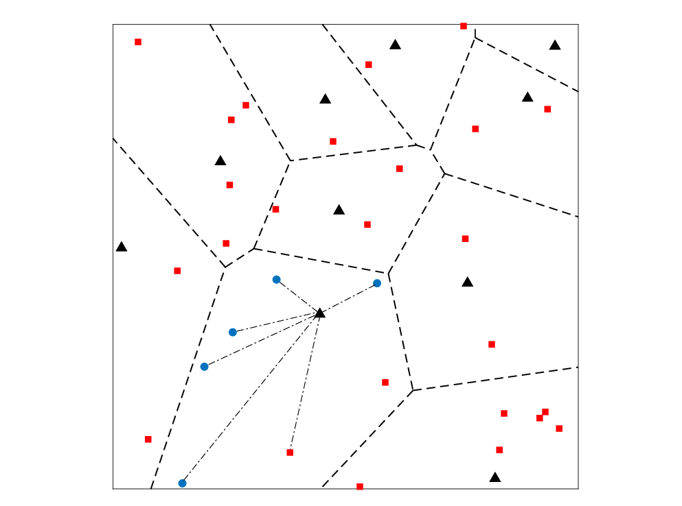
From above discussions and accounting for the power control scheme in (1), the superimposed signal received at the typical BS can be generally expressed as (3), where $\mathcal{U}_{in}$ is the set of active UEs with pilot collisions in a specific Vironoi cell, $\mathcal{U}$ is the set of UEs that can be decoded by using MPA, and they are identified by the subscript “j’’¹¹ 1 In general, we have $|\mathcal{U}|\leq J$, and if $|\mathcal{U}|<J$, $J-|\mathcal{U}|$ all-zero codewords should be involved in MPA as reported in [31]. Note that the cardinality of $\mathcal{U}$ can be formulated as

In addition, $\mathbf{z}_{o}$ is the noise vector that consists of complex Gaussian random variables with distribution $\mathcal{CN}(0,\sigma^{2})$. In addition, $D_{i}$ is the distance between $\text{BS}_{o}\in\Phi_{B}$ and $\text{UE}_{i}\in\Phi_{UE}$, and $\mathds{1}\left\{\cdot\right\}$ denotes an indicator function takes value 1 if the condition $\mathds{1}\left\{\cdot\right\}$ is satisfied. According to (3), a general expression for the SINR of $\text{BS}_{o}$ can be formulated as

where $\mathcal{G}_{j}=\sum_{s=1}^{d_{s}}|c_{j,s}|^{2}|h_{j}^{(s)}|^{2}=\sum_{s=1}^{d_{s}}|g_{j}^{(s)}|^{2}$, in which $g_{j}^{(s)}$ is the $s$th entry of $\mathbf{c}_{j}\text{diag}(\mathbf{h}_{j})\in\mathbb{C}^{1\times K}$. $\mathcal{I}_{intra}$ and $\mathcal{I}_{inter}$ denote the intra- and inter-cell interference, respectively. Furthermore, it should be noted that $\mathcal{G}_{u}=\sum_{s=1}^{d_{s}}|g_{u}^{(s)}|^{2}$ and $\mathcal{G}_{i}=\sum_{s=1}^{d_{s}}|g_{i}^{(s)}|^{2}$ have the same formulation as $\mathcal{G}_{j}$. As the channel response coefficient follows complex Gaussian distribution, and thus $\mathcal{G}_{\Xi}\sim\text{Gamma}(d_{s},1)$, in which $\Xi\in\{j,u,i\}$. For simplicity, we also define $\mathbf{H}_{\Xi}=\text{diag}(\mathbf{h}_{\Xi})$, $b=\frac{\eta}{2}$, and $P_{i}=\rho R_{i}^{\eta}$ in the following of this paper.

Moreover, it can be also observed from (3) that useful signals are superimposed by at most $J$ RA UEs in a typical cell. As a result, the intra-cell interference exists only when the number of active UEs is larger than that of supported UEs for a GF-SCMA system, and thus the number of intra-cell interferes equals to $\left|\mathcal{U}_{in}\right|-J$. Remind that this is because MPA is unable to decode SCMA codewords once reaching the maximum number of supported UEs. As such, an important assumption should be made in this work, which is demonstrated as follows. As depicted in Fig. 2, taking account for a network where the intensity of UE is $\lambda_{u}^{{}^{\prime}}=p_{a}\lambda_{ue}/JL$. We consider a typical cell in which randomly selected $|\mathcal{U}|$ UEs are assumed to have distinguished CTUs. In this case, we assume that the remaining UEs have the same pilot as one of the $|\mathcal{U}|$ UEs, such that the realistic intensity of interferes $\lambda_{u}$ is approximated as the intensity of UE that has the same pilot, i.e., $\lambda_{u}\approx\lambda_{u}^{{}^{\prime}}$. The feasibility of such an approximation is verified in Section. V.

From the previous discussion, it is important to note that the key factors influencing the success probability can be outlined as follows: 1) Only RA UEs without experiencing pilot collisions have the opportunity for BS to recover the transmitted data; hence, the interference come from UEs with the same pilot; 2) The signal of RA UEs transmitting with GF-SCMA cannot be recognized by its serving BS, since its lower received SINR than the SINR threshold $\gamma_{\text{th}}$, such that outage occurs; 3) As MPA is utilized to recover the data of each UE in GF-SCMA, the interference comes from intra- and inter-cell superimpose on the signals of at most $J$ UEs that are multiplexed by $T$ RBs.

In the sequel, the mathematical expression of success probability is derived by taking the above influencing factors and the approximation in Sec. II-D into account. To apply Gil-Palaez inversion theorem to calculate success probability[32, 33], we first consider the characteristic function (CF) of the interference according to (3), and the definition of SINR in (5). Here, we assume that the data of UEs belong to $\mathcal{U}$ can be perfectly decoded; hence, we have following lemma.

respectively, where $\mathcal{M}_{\omega}=1-{}_{2}F_{1}(-\frac{1}{b},d_{s};1-\frac{1}{b};j\omega\rho)$²² 2 Unless otherwise stated, ${}_{p}F_{q}$, where $p$ and $q$ are two nonnegative integers, denotes the generalized generalized hypergeometric functions in this paper., $\alpha=\pi\lambda_{b}\left(\rho_{m}/\rho\right)^{1/b}$, $\beta=(\mathcal{O}_{p}\lambda_{u}/c\lambda_{b})$, and $c=3.575$ is a constant related to the approximate probability mass function of the HPPP Voronoi cell. $\mathcal{K}_{\omega}=\mathbb{E}\left[\exp\left(j\omega\mathcal{G}_{\Xi}\right)\right]=(1-j\omega\rho)^{-d_{s}}$, and $\mathcal{O}_{p}=exp\left(-\alpha\right)$ is the truncation outage probability.

Proof. See Appendix. A.

Note that, to provide a general analytical framework of GF-SCMA, the inter- and intra-cell interference are both considered. Remind that the interference comes from the reuse of pilot in CTUs. According to the discussion in Sec. II, we define a success transmission as the nonexistence of pilot collision and SINR at the receiver satisfies $\text{SINR}\geq\gamma_{\text{th}}$, and thus the following theorem can be given:

Proof. See Appendix. B.

In Theorem 1, we can observe that when considering full channel inversion power control without truncation, $\Phi_{\mathcal{I}_{inter}}$, $\Phi_{\mathcal{I}_{intra}}$ and $\mathcal{S}_{\omega}$ can be further simplified by substituting $\mathcal{O}_{p}\to 1$ and $\exp\left(-\alpha\right)\to 0$. This follows from the fact that $\rho_{m}\to\infty$, such that $\alpha\to\infty$. In the following subsection, we will provide some key properties of the success probability, which will be verified in Section. V via numerical results.

In SCMA, the codebook design method is the main characteristic that distinguishes it from other multiple access schemes. In this regard, it is necessary to study the influence of $d_{s}$ on the success probability. To this end, we provide the following two corollaries.

Proof: See Appendix C.

It can be seen that $\sqrt{\xi}$ and $\exp\left(-(\lambda_{u}/\lambda_{b})^{2}\xi\right)$ have different monotonicity. Nevertheless, as is shown in (30), when $\lambda_{u}/\lambda_{b}$ is relatively low, it can be inferred from Corollary 1 that codewords with relatively large $d_{s}$ is more probable to have superiority over the sparser ones, especially in the region of low and medium detection threshold. To elaborate further, the following conclusions are given based on Corollary 1.

Proof: We first prove (10). Based on the proof of Corollary 1, when $d_{s}\to\infty$, $\mathcal{S}_{\omega}\to\left(1+\beta\right)^{-c-1}$, such that $P_{\text{suc}}$ scales with $\xi^{1/2}$, which is uncorrelated to other parameters. After that, when $d_{s}\to\infty$, we have $\xi^{1/2}\to 1$, and thus (10) is satisfied. As for (11), it can be directly inspected by substituting $d$ and $d_{s}+d$ into (30). This concludes the proof.

According to the results in these two corollaries, we can have the following implications: 1) Although the success probability of GF-SCMA benefits from the increase of sparsity degree $d_{s}$ at low and medium $\gamma_{\text{th}}$ region when a large number of UE is deployed, no performance gain can be enjoyed by making the codebook denser³³ 3 In general, there are two approaches to increase $d_{s}$ in SCMA without changing $J$. One is to adjust $K$ and $T$ as the increase of $d_{s}$, the other is to adopt novel codebook design rules, such as density code multiple access (DCMA), which is recently proposed in [34], and the sparse degree $d_{s}=K$.. This property is important for the design of codebook with large $J$ and $K$; 2) According to (11), the performance gap between the sparse and dense codebooks shrinks as the increase of detection threshold. This property means that the codebooks of GF-SCMA with larger $d_{s}$ are able to achieve higher success probability in the region of low and medium $\gamma_{\text{th}}$, which is useful in the design of practical system; 3) It can be seen from (30), as the increase of $\lambda_{u}/\lambda_{b}$, the impact of $d_{s}$ on $P_{\text{suc}}$ is negligible, and thus the gap between $P_{\text{suc}}$ and $P_{\text{suc}}\left(d_{s}+d\right)$ becomes marginal. In a word, it can be inferred that a denser deployment of UEs reduces the influence of codebook design in the GF-SCMA system. Besides, based on Theorem 1, another interesting property can be obtained, which is demonstrated as follows,

Proof: Similar to the proof in Corollary 1, according to the approximation in (30), it can be inferred that $P_{\text{suc}}\left(\lambda_{u}\right)-P_{\text{suc}}(\lambda_{u}^{{}^{\prime}})$ mainly depends on the function $f(x)=\xi^{1/2}x-x/\gamma_{\text{th}}\exp(-\xi x^{2})$, where $x$ is a variable proportional to $\lambda_{u}$ here. By studying the first-order derivative of $f(x)$, i.e., $f^{{}^{\prime}}(x)=\xi^{1/2}-1/\gamma_{\text{th}}\exp(-\xi x^{2})(1-2\xi x^{2})$, we can observe that the monotonicity of $f(x)$ changes at a stationary point $x>0$. On the other hand, by direct inspection of the equation $f^{{}^{\prime}}(x)=0$, the stationary point $x$ increases by decreasing $\gamma_{\text{th}}$. This completes the proof.

This result actually is not quite straightforward because using a fixed number of BSs to support more UEs should reduce the success probability intuitively. An intuitive explanation of this property is that even though more UEs are deployed in the network when $\lambda_{u}$ is relatively high, in this case, $|\mathcal{U}|$ approximately equals to $J$ on average, and thus the aggregate interference of UEs belong to $\mathcal{U}$ is also high. For the case when $\lambda_{u}$ is low, although less interference is undergone, the aggregate power of superimposed signal in $\mathcal{U}$ is also low. Since $|\mathcal{U}|$ is more probable to be small with low $\lambda_{u}$, and thus leading to a fail transmission in the region of low $\gamma_{\text{th}}$.

Furthermore, after attaining success probability, the ASE of GF-SCMA network can be also derived by using

where $\bar{\mathcal{U}}$ is the mean number of served UEs, which can be further written as:

It should be noted that the ASE and success probability depict two different aspects of a communication system. A higher success probability means that the UEs can transmit data more reliable so that they enjoy a better quality of experience, whereas ASE denotes the spatial reuse efficiency, and thus more UEs can be supported in a network with a higher ASE.

It is known that the codewords of SCMA are well designed according to the method presented in [35], and thus the UEs that use different codebooks can recover the data with high reliability. Even though the effect of reusing the same codebook for different UEs can be mitigated due to the application of advanced MUD (i.e. MPA) and the reciprocity of wireless channel in GF-SCMA. However, it also causes error rate degradation [36, 26, 18]. Thereby, the codebook collision is deemed to be the main influencing factor of the error rate performance of GF-SCMA, especially in a large-scale network. Motivated by such facts, we examine the error rate performance of GF-SCMA in the case of codebook collision. Although errors occur even though different codebooks are utilized in link-level simulations [29], the error rate performance deteriorates significantly when the same codebooks are utilized. Therefore, we can conclude that the error rate performance of GF-SCMA is mainly determined by codebook collisions in the considering model.

Similar to the analysis in Section. III-A, it is assumed that MPA can perfectly cancel the interference when $|\mathcal{U}|\leq J$. Besides, we only consider the case that the same codebook is reused at most once for tractability. That is, we end up with a maximum of one collided UE per BS. The rationale behind such an assumption follows from the fact that each cell shares the same codeword pool in GF-SCMA, and user-specific codebooks are assigned to the active UEs in each cell. Furthermore, taking into account the sporadic communication in massive IoT networks, the probability of reusing the same codebook more than once by different UEs is very low. This can be explained by the fact that the number of codebook $J$ is sufficient to support all UEs in a cell in most cases. Therefore, each BS is assumed to serve at most one UE using the same codebook. In a word, the derived results in this section intends to reveal the error rate performance when CTU collision occurs in a GF-SCMA system, this can help to examine the robustness of GF-SCMA under overloading condition.

It is acknowledged that various MPA based algorithms can be applied to the detection of SCMA. Therefore, to provide a unified analytical model for the error performance, an optimal receiver, i.e., maximum likelihood detector (MLD) is considered in this work. In addition, we intend to compute the average symbol error probability (ASEP) from APEP, which has been utilized to evaluate the SCMA error rate performance in the single-cell with a fixed number of randomly deployed users in [13, 37, 38].

For GF-SCMA, the MLD with perfect channel state information (CSI) at the receiver’s side can be formulated as

where $\|\cdot\|$ represents the Euclidean distance. According to the definition of PEP, the PEP of SCMA codeword in a GF-SCMA network can be written as

where ($\mathnormal{a}$) follows from defining $\mathcal{V}=\mathcal{I}_{inter}+\mathbf{z}_{o}$, $\mathbf{\Delta}_{o}=\mathbf{c}_{o}-\tilde{\mathbf{c}_{o}}$, and ($\mathnormal{b}$) holds because $\mathcal{V}$ is a circularly symmetric random variable (RV), $\Re\left\{\cdot\right\}$ denotes the real part of a complex number, and $\dagger$ is the conjugate transpose of a complex vector. $F_{\bar{\mathcal{V}}}$ is the cumulative density function (CDF) of $\bar{\mathcal{V}}=\mathcal{V}\left(\mathbf{\Delta}_{o}\mathbf{H}_{o}\right)^{\dagger}$. For simplicity, we define $\mathcal{Z}=\mathbf{z}_{o}\left(\mathbf{\Delta}_{o}\mathbf{H}_{o}\right)^{\dagger}$, and $\mathcal{I}=\mathcal{I}_{inter}\left(\mathbf{\Delta}_{o}\mathbf{H}_{o}\right)^{\dagger}$, such that $\Re\left\{\mathcal{Z}\right\}$ has the same distribution as $\mathcal{V}$. By using Gil-Palaez inversion theorem, $F_{\bar{\mathcal{V}}}$ can be re-written as:

where $\Phi_{\bar{\mathcal{V}}}$ is the CF of $\bar{\mathcal{V}}$, and $\mathcal{H}=\|\mathbf{\Delta}_{o}\mathbf{H}_{o}\|^{2}$. Therefore, to calculate the PEP of GF-SCMA, the CF of $\mathcal{\bar{V}}$ should be calculated. According to the previous definition of $\mathcal{Z}$ and $\mathcal{I}$, $\Phi_{\bar{\mathcal{V}}}$ can be decomposed into $\Phi_{\bar{\mathcal{V}}}=\varphi_{\mathcal{I}}\varphi_{\mathcal{Z}}$, where $\varphi_{\mathcal{Z}}$ and $\varphi_{\mathcal{I}}$ are the CFs of RV $\mathcal{Z}$ and $\mathcal{I}$, respectively. It should be noted that $\mathcal{Z}$ is also a complex Gaussian distributed RV, and thus $\varphi_{\mathcal{Z}}=\exp\left\{-\frac{1}{4}\omega^{2}\sigma^{2}\mathcal{H}\right\}$. The following Lemma 2 will calculate $\varphi_{\mathcal{I}}$.

Proof. See Appendix. D.

Note that when $\rho_{m}\to\infty$, we have $\gamma(2,\pi\lambda_{b}(\frac{\rho_{m}}{\rho})^{1/b})\to 1$, such that $C\to 1$. According to (15), it can be concluded that PEP of GF-SCMA is equivalent to the CDF of $\bar{\mathcal{V}}$; hence, based on Lemma 2, the APEP is given in the following theorem.

where $\Gamma\left(\cdot\right)$ denotes the gamma funtion.

Proof. See Appendix. E.

According to the APEP result in Theorem 2, we can have the following remark:

Remark 1. The APEP decreases by increasing $\lambda_{b}$. This property can be simply explained by (19). As $C$ is determined by $\lambda_{b}$; hence, APEP decreases exponentially with $\lambda_{b}$ according to (19). Similarly, it can be also inferred that the APEP decreases by increasing $\rho_{m}$.

So far, the APEP of GF-SCMA system under codebook collision is obtained, in the sequel, the error rate performance will be presented based on APEP analysis.

To compute ASEP from APEP, a union bound on the ASEP is given by [13]

where $M$ is the cardinality of $\mathcal{C}$. Note that $M^{2}$ PEPs should be calculated according to (21), and thus the computational complexity will be high especially when $M$ is large. In this paper, to provide a simpler to compute formulation with high accuracy, we utilize an approximation under the equal-probable transmission codeword assumption [13]. The approximation follows from the fact that the nearest neighbors among the codeword pair $(\tilde{\mathbf{c}_{o}},\mathbf{c}_{o})$ dominate the error rate in high SNR region. So, to reduce the number of PEPs that should be calculated, we can only consider the nearest neighbors of each codeword with minimum Euclidean distance, which has main contribution to the ASEP performance. Accordingly, the ASEP of GF-SCMA can be formulated as

where $\|\mathbf{\Delta}_{\min}\|^{2}=\min_{\mathbf{c}_{o},\tilde{\mathbf{c}_{o}}\in\mathcal{C}}\{\|\mathbf{c}_{o}-\tilde{\mathbf{c}_{o}}\|^{2},\mathbf{c}_{o}\neq\tilde{\mathbf{c}_{o}}\}$ represents the minimum Euclidean distance among all codeword pairs $(\tilde{\mathbf{c}_{o}},\mathbf{c}_{o})$, and $\mathcal{N}_{\mathbf{c}_{o}}$ is the number of the nearest neighbors of $\mathbf{c}_{o}$. $P(\tilde{\mathbf{c}_{o}}\to\mathbf{c}_{o})\mid_{\mathbf{\Delta}_{\min}}$ denotes the PEP by replacing $\mathbf{\Delta}_{\min}$ with $\mathbf{\Delta}_{o}$. The accuracy of such an approximation will be verified in Section. V.

To elaborate further, some ASEP trends can be obtained based on the analysis, and thus we have the following two remarks. We have to point out that these two remarks are based on the assumption that $\text{SNR}\to\infty$ and $\rho_{m}\to\infty$. This indicates that an interference-limited and full channel inversion power control is considered in the following discussions.

Remark 2. When $\text{SNR}\to\infty$, the ASEP is independent of $\rho$. It can be observed from (19) that if $\text{SNR}\to\infty$, then $\frac{v}{4\text{SNR}}\to 0$, and $C\to 1$. Thereby, the ASEP is only determined by (20) and path-loss exponent $\eta$. This property implies that an error-floor emerges at very high SNR region when full channel inversion power control without truncation is utilized.

Remark 3. Higher $b$ (or equivalently $\eta$) leads to a worse error rate performance. To explain this property, the monotonicity of ${}_{1}F_{1}(-1/b;1-1/b;-v/4)$ should be investigated. As can be seen in (32), $(-1/b)_{q}/(1-1/b)_{q}$ reflects the impact of $b$ on ${}_{1}F_{1}(-1/b;1-1/b;-v/4)$, in which $(-1/b)_{q}/(1-1/b)_{q}$ can be further simplified as $1/(1-qb)$, which follows from $\Gamma(z+1)=z\Gamma(z)$. As $q$ is a non-negative integer, and thus $(-1/b)_{q}/(1-1/b)_{q}$ is proportional to $-1/b$.

References

- [1] P. Schulz, M. Matthe, H. Klessig et al., “Latency critical IoT applications in 5G: Perspective on the design of radio interface and network architecture,” IEEE Communications Magazine, vol. 55, no. 2, pp. 70–78, Feb. 2017.
- [2] H. S. Dhillon, H. Huang, and H. Viswanathan, “Wide-area wireless communication challenges for the Internet of Things,” IEEE Communications Magazine, vol. 55, no. 2, pp. 168–174, Feb. 2017.
- [3] L. Chettri and R. Bera, “A comprehensive survey on Internet of Things (IoT) toward 5G wireless systems,” IEEE Internet of Things Journal, vol. 7, no. 1, pp. 16–32, Jan. 2020.
- [4] L. Dai, B. Wang, Z. Ding, Z. Wang, S. Chen, and L. Hanzo, “A survey of non-orthogonal multiple access for 5G,” IEEE Communications Surveys and Tutorials, vol. 20, no. 3, pp. 2294–2323, 3rd quarter. 2018.
- [5] J. Tang, J. Luo, M. Liu et al., “Energy efficiency optimization for NOMA with SWIPT,” IEEE Journal of Selected Topics in Signal Processing, vol. 13, no. 3, pp. 452–466, Jun 2019.
- [6] P. Xu, Y. Wang, G. Chen et al., “Design and evaluation of buffer-aided cooperative NOMA with direct transmission in IoT,” IEEE Internet of Things Journal, vol. PP, no. 99, pp. 1–1, Early Access 2020.
- [7] M. Alkhawatrah, Y. Gong, G. Chen, S. Lambotharan, and J. A. Chambers, “Buffer-aided relay selection for cooperative NOMA in the Internet of Things,” IEEE Internet of Things Journal, vol. 6, no. 3, pp. 5722–5731, Jun. 2019.
- [8] Y. Saito, Y. Kishiyama, A. Benjebbour et al., “Non-orthogonal multiple access (NOMA) for cellular future radio access,” in Proc. IEEE 77th Vehicular Technology Conference (VTC Spring), Dresden,Germany, Jun. 2013, pp. 1–5.
- [9] M. B. Shahab, R. Abbas, M. Shirvanimoghaddam, and S. J. Johnson, “Grant-free non-orthogonal multiple access for IoT: A survey,” IEEE Communications Surveys & Tutorials, vol. 22, no. 3, pp. 1805–1838, 3rd quarter. 2020.
- [10] X. Jian, Y. Liu, Y. Wei, X. Zeng, and X. Tan, “Random access delay distribution of multichannel slotted ALOHA with its applications for machine type communications,” IEEE Internet of Things Journal, vol. 4, no. 1, pp. 21–28, Feb. 2017.
- [11] R. Harwahyu, R. G. Cheng, C. H. Wei, and R. F. Sari, “Optimization of random access channel in NB-IoT,” IEEE Internet of Things Journal, vol. 5, no. 1, pp. 21–28, Feb. 2018.
- [12] J. Chen, Z. Wang, W. Xiang, and S. Chen, “Outage probability region and optimal power allocation for uplink SCMA systems,” IEEE Transactions on Communications, vol. 66, no. 10, pp. 4965–4980, Oct. 2018.
- [13] J. Bao, Z. Ma, M. Xiao, Z. Ding, and Z. Zhu, “Performance analysis of uplink scma with receiver diversity and randomly deployed users,” IEEE Transactions on Vehicular Technology, vol. 67, no. 3, pp. 2792–2797, Mar. 2018.
- [14] Z. Yang, X. Lei, Z. Ding, P. Fan, and G. K. Karagiannidis, “On the uplink sum rate of SCMA system with randomly deployed users,” IEEE Wireless Communications Letters, vol. 6, no. 3, pp. 338–341, Jun. 2017.
- [15] S. Han, X. Tai, W. Meng, and C. Li, “A resource scheduling scheme based on feed-back for SCMA grant-free uplink transmission,” in 2017 IEEE International Conference on Communications (ICC), Paris,France, Jul. 2017, pp. 1–6.
- [16] S. Moon, H. Lee, and J. Lee, “SARA: Sparse code multiple access-applied random access for IoT devices,” IEEE Internet of Things Journal, vol. 5, no. 4, pp. 3160–3174, Aug. 2018.
- [17] F. Wei, W. Chen, Y. Wu, J. Ma, and T. A. Tsiftsis, “Message-passing receiver design for joint channel estimation and data decoding in uplink grant-free SCMA systems,” IEEE Transactions on Wireless Communications, vol. 18, no. 1, pp. 167–181, Jan. 2019.
- [18] J. Zhang, L. Lu, Y. Sun et al., “PoC of SCMA-based uplink grant-free transmission in UCNC for 5G,” IEEE Journal on Selected Areas in Communications, vol. 35, no. 6, pp. 1353–1362, Jun. 2017.
- [19] N. Ye, X. Li, H. Yu, A. Wang, W. Liu, and X. Hou, “Deep learning aided grant-free NOMA toward reliable low-latency access in tactile Internet of Things,” IEEE Transactions on Industrial Informatics, vol. 15, no. 5, pp. 2995–3005, May. 2019.
- [20] Y. Liu, Y. Deng, H. Zhou, M. Elkashlan, and A. Nallanathan. (2021, Jan.) A general deep reinforcement learning framework for grant-free NOMA optimization in mURLLC. [Online]. Available: https://arxiv.org/abs/2101.00515.pdf
- [21] L. Liu, M. Sheng, J. Liu, X. Wang, and J. Li, “Success probability and area spectral efficiency in SCMA wireless networks,” IEEE Transactions on Vehicular Technology, vol. 67, no. 8, pp. 7764–7768, Aug. 2018.
- [22] J. V. C. Evangelista, Z. Sattar, and G. Kaddoum, “Analysis of contention-based SCMA in mMTC networks,” in 2019 IEEE Latin-American Conference on Communications (LATINCOM), Salvador,Brazil, Nov. 2019, pp. 1–6.
- [23] J. Liu, M. Sheng, L. Liu, Y. Shi, and J. Li, “Modeling and analysis of SCMA enhanced D2D and cellular hybrid network,” IEEE Transactions on Communications, vol. 65, no. 1, pp. 173–185, Jan. 2017.
- [24] R. Abbas, M. Shirvanimoghaddam, Y. Li, and B. Vucetic, “A novel analytical framework for massive grant-free NOMA,” IEEE Transactions on Communications, vol. 67, no. 3, pp. 2436–2449, Mar. 2019.
- [25] X. Yue, Z. Qin, Y. Liu, S. Kang, and Y. Chen, “A unified framework for non-orthogonal multiple access,” IEEE Transactions on Communications, vol. 66, no. 11, pp. 5346–5359, Nov. 2018.
- [26] L. Lu, Y. Chen, W. Guo, H. Yang, Y. Wu, and S. Xing, “Prototype for 5G new air interface technology SCMA and performance evaluation,” China Communications, vol. 12, no. Supplement, pp. 38–48, Dec. 2015.
- [27] H. ElSawy and E. Hossain, “On stochastic geometry modeling of cellular uplink transmission with truncated channel inversion power control,” IEEE Transactions on Wireless Communications, vol. 13, no. 8, pp. 4454–4469, Aug. 2014.
- [28] M. Haenggi, Ed., Stochastic Geometry for Wireless Networks: Percolation, connectivity, and coverage. Cambridge, U.K: Cambridge University Press, 2012.
- [29] H. Nikopour and H. Baligh, “Sparse code multiple access,” in Proc. IEEE 24th Int. Symp. Pers. Indoor Mobile Radio Commun. (PIMRC), London, United Kingdom, Sep. 2013, pp. 332–336.
- [30] M. Vameghestahbanati, I. D. Marsland, R. H. Gohary et al., “Multidimensional constellations for uplink SCMA systems — A comparative study,” IEEE Communications Surveys & Tutorials, vol. 21, no. 3, pp. 2169–2194, Apr. 2019.
- [31] K. Au, L. Zhang, H. Nikopour et al., “Uplink contention based SCMA for 5G radio access,” in 2014 IEEE Globecom Workshops (GC Wkshps), Austin, TX, USA, Dec. 2014, pp. 900–905.
- [32] J. Gil-Pelaez, “Note on the inversion theorem,” Biometrika, vol. 38, no. 3/4, pp. 481–482, Dec. 1951.
- [33] N. Deng and M. Haenggi, “SINR and rate meta distributions for HCNs with joint spectrum allocation and offloading,” IEEE Transactions on Communications, vol. 67, no. 5, pp. 3709–3722, May. 2019.
- [34] Z. Liu and L.-L. Yang. (2020, Sep.) Sparse or dense: A comparative study of code-domain NOMA systems. [Online]. Available: https://arxiv.org/pdf/2009.04148.pdf
- [35] M. Taherzadeh, H. Nikopour, A. Bayesteh, and H. Baligh, “SCMA codebook design,” in in Proc. IEEE Veh. Technol. Conf. (VTC-Fall), Vancouver, BC, Canada, Sep. 2014, pp. 1–5.
- [36] Y. Yang, Y. Zhao, and D. Li, “SCMA uplink decoding with codebook collision,” in 2017 IEEE 86th Vehicular Technology Conference (VTC-Fall), Toronto, ON, Canada, 2017, pp. 1–5.
- [37] J. Bao, Z. Ma, G. K. Karagiannidis, M. Xiao, and Z. Zhu, “Joint multiuser detection of multidimensional constellations over fading channels,” IEEE Transactions on Communications, vol. 65, no. 1, pp. 161–172, Jan. 2017.
- [38] K. Lai, J. Lei, L. Wen, and G. Chen, “Codeword position index modulation design for sparse code multiple access system,” IEEE Transactions on Vehicular Technology, vol. 69, no. 11, pp. 13 273–13 288, Nov 2020.
- [39] Y. Liang, X. Li, and M. Haenggi, “Non-orthogonal multiple access (NOMA) in uplink poisson cellular networks with power control,” IEEE Transactions on Communications, vol. 67, no. 11, pp. 8021–8036, Nov. 2019.
- [40] I. S. Gradshteyn and I. M. Ryzhik, Eds., Table of integrals, series, and products, 7th Edition. USA: Academic Press, 2007.
- [41] N. Jiang, Y. Deng, X. Kang, and A. Nallanathan, “Random access analysis for massive iot networks under a new spatio-temporal model: A stochastic geometry approach,” IEEE Transactions on Communications, vol. 66, no. 11, pp. 5788–5803, Nov. 2018.