Quantum interferometry for rotation sensing in an optical microresonator

Weijun Cheng Affiliation: Center for Quantum Sciences and School of Physics, Northeast Normal University, Changchun 130024, China Zhihai Wang Email: wangzh761@nenu.edu.cn Affiliation: Center for Quantum Sciences and School of Physics, Northeast Normal University, Changchun 130024, China Xiaoguang Wang Email: xgwang1208@zju.edu.cn Affiliation: Zhejiang Institute of Modern Physics, Department of Physics, Zhejiang University, Hangzhou 310027, China

Abstract

We theoretically propose a scheme to perform rotation sensing in a whispering-gallery-mode resonator setup. With the assistance of a large detuned two-level atom, which induces the effective coupling between clockwise and counterclockwise propagating modes in the resonator, we realize an effective interferometry with SU(2) algebraic structure. By studying the quantum Fisher information of the system, we find that the estimate accuracy for the angular velocity of the rotation can achieve and even break the Heisenberg limit in linear and nonlinear setup, respectively. The high performance of quantum metrology is proved to be associated with the state compressibility during the time evolution. We hope that our investigation will be useful in the design of a quantum gyroscope based on spinning resonators.

I introduction

The ultraprecise estimation of parameters, which is introduced in the quantum interferometry Caves1; Caves2, has been widely promoted to the optical microresonator. The theory claims that the quantum features such as entanglement and squeeze can dramatically enhance the interferometer sensitivity V. Giovannetti1; V. Giovannetti2; D. W. Berry; J. Joo. In this community, the phase sensitivity of interferometer can approach the Heisenberg limit with $\Delta x\sim 1/n$ ( $n$ is the amount of the source employed) scaling, which is much better than the classical astrict, named the standard quantum limit with $\Delta x\sim 1/\sqrt{n}$ scaling.

The quantum interferometry is achieved by measuring the intensity difference at the output of interferometer H. S. Eisenberg; Itai A; K. J. Resch; D. Leibfried. Typically, the sensitivity enhancements in different types of interferometric schemes have been proposed in many setups, such as Sagnac, Mach-Zehnder, Fabry-Pérot and SU(1,1) interferometers K. X. Sun; A. N. Boto; S. J. Bentley; S. H. Tan; V. Giovannetti; M. Tsang; S. Lloyd; G. Khoury; S. D. Huver; B. Yurke. Nowadays, instead of exploring quantum metrology in the interferometer, quantum sensors composed by for example quantum dot and cavity QED system have made great achievements M. Kasevich; C. E. Wieman; Xiaoming; Fang; FFujimoto; 71; 72; MW1; LR; 61; 62. As one kind of the simple two-mode resonant cavities, the whispering-gallery-mode (WGM) resonator has become a versatile platform for measuring the angular velocity based on Sagnac effect Karl; CDV.

The WGM supports the clockwise and counterclockwise propagating optical modes, and the effective coupling between the two optical modes can be induced by coupling to a large detuned two-level atom. Adiabatically eliminating the degree of freedom of the atom, we construct an effective interferometer with SU $(2)$ Lie algebra structure in this paper. It is thus similar to the Mach-Zehnder interferometer and supplies us a way to perform the rotating sensing. The underlying physics is to transform the information about the angular velocity to the phase difference of the two optical modes. The study about the quantum Fisher information (QFI) shows that the effective inter-mode coupling, which encodes the information of rotation into both of the amplitudes and the phases of the wave function, plays a decisive role in achieving the Heisenberg limit for the estimation of angular velocity. Moreover, we find that even a weak non-linearity in the system will further enhance the quantum metrology and defeat the Heisenberg limit by achieving a $1/n^{3}$ scaling for the QFI. We explain the enhancement by the compressibility of state distribution during the time evolution.

The rest of the paper is organized as follows. In Sec. II, we review quantum interferometry and present a feasible experimental scheme in the WGM optical microresonator. In Sec. 2, we discuss the effect of the nonlinearity in the system for enhancing the quantum metrology. In Sec. IV, we give a short summary. In the appendix, we present some detailed calculations.

II Model and Hamiltonian

II.1 Mach-Zehnder Interferometer

Refer to caption — Figure 1: (a) Schematic diagram of the Mach-Zehnder interferometer. It consists of two $50-50$ beam splitters: $S_{1}$ and $S_{2}$ , the relative phase shift device $\phi=\phi_{2}-\phi_{1}$ and the photodetectors: $D_{1}$ and $D_{2}$ . (b) Sketch of a rotating whispering-gallery-mode optical resonator, which couples to a large detuned two-level atom.

Let us first review the Mach-Zehnder interferometer, which is sketched in Fig. 1(a). It consists of two $50-50$ beam splitters: $S_{1}$ and $S_{2}$ , the relative phase shift device $\phi=\phi_{2}-\phi_{1}$ and the photodetectors: $D_{1}$ and $D_{2}$ . It is convenient to introduce the Schwinger representation for a two-mode quantized light field, that is

$\displaystyle J_{x}$	$\displaystyle=$	$\displaystyle\frac{1}{2}(ab^{\dagger}+a^{\dagger}b),$
$\displaystyle J_{y}$	$\displaystyle=$	$\displaystyle\frac{1}{2i}(ab^{\dagger}-a^{\dagger}b),$
$\displaystyle J_{z}$	$\displaystyle=$	$\displaystyle\frac{1}{2}(a^{\dagger}a-b^{\dagger}b),$
$\displaystyle J^{2}$	$\displaystyle=$	$\displaystyle J^{2}_{x}+J^{2}_{y}+J^{2}_{z},$	(1)

and

\displaystyle N

\displaystyle=

\displaystyle a^{\dagger}a+b^{\dagger}b.

(2)

Here $a$ and $b$ represent the annihilation operation of two beams and the commutation relations satisfy the Lie algebra of SU(2):

\displaystyle[J_{x},J_{y}]=iJ_{z},[J_{y},J_{z}]=iJ_{x},[J_{z},J_{x}]=iJ_{y}.

(3)

It then yields

	$\displaystyle J_{z}\|j,m\rangle$	$\displaystyle=$	$\displaystyle m\|j,m\rangle,$
	$\displaystyle J^{2}\|j,m\rangle$	$\displaystyle=$	$\displaystyle j(j+1)\|j,m\rangle,$		(4)

and

\displaystyle N|j,m\rangle

\displaystyle=

\displaystyle n|j,m\rangle,

(5)

where $n=2j$ is the total number of photons and $m$ is the difference of photon number between the two ports.

For the sake of convenience, here and after, we set the entangled initial state as $|in\rangle=(|j,0\rangle+|j,1\rangle)/\sqrt{2}$ . In the Schrödinger picture, the devices $S_{1}$ , $S_{2}$ and $\phi=\phi_{2}-\phi_{1}$ will lead to transformations $\exp(-i\pi J_{x}/2)$ , $\exp(i\pi J_{x}/2)$ and $\exp(-i\phi J_{z})$ , respectively. The final state $|out\rangle$ is thus

\displaystyle|out\rangle

\displaystyle=

\displaystyle U(\phi)|in\rangle=e^{i\frac{\pi}{2}J_{x}}e^{-i\phi J_{z}}e^{-i\frac{\pi}{2}J_{x}}|in\rangle.

(6)

As an interferometer, the phase difference $\phi$ is the parameter to be estimated. In the field of quantum metrology, the QFI is a central quantity, giving a theoretically achievable limit on the precision for an unknown estimated parameter $\phi$ . Considering the parameter $\phi$ as a random variable the mean square fluctuation of $\phi$ is defined as $\Delta\phi=\sqrt{\bar{\phi^{2}}-\bar{\phi}^{2}}$ . According to the quantum Cramér-Rao inequality, $\Delta\phi$ is bounded by JA; RR; SL1; SL2

\displaystyle\Delta\phi\geq\frac{1}{\sqrt{\nu\mathcal{F}_{\phi}}},

(7)

where $\nu$ is the times of the independent measurements and $\mathcal{F}_{\phi}$ is the QFI with respective to $\phi$ . For a general quantum pure state $|\psi\rangle$ , the QFI is given by

\displaystyle\mathcal{F}_{\phi}=4(\langle\partial_{\phi}\psi|\partial_{\phi}\psi\rangle-|\langle\psi|\partial_{\phi}\psi\rangle|^{2}).

(8)

Introducing a Hermitian operator

\mathcal{H}=-iU^{\dagger}(\partial U/\partial\phi)

(9)

( $U$ is the evolution operation), the QFI can be reduced to

\displaystyle\mathcal{F}_{\phi}=4\langle\Delta^{2}\mathcal{H}\rangle,

(10)

where $\Delta^{2}\mathcal{H}=\langle\mathcal{H}^{2}\rangle-\langle\mathcal{H}\rangle^{2}$ .

Then we have

\displaystyle\mathcal{F}_{\phi}=2j(j+1)-1,

(11)

so that $\Delta\phi\simeq\sqrt{2}/n$ , that is, the fluctuation of $\phi$ is proportional to $1/n$ , which refers as the Heisenberg limit. Furthermore, we note that the QFI will decline dramatically to $1$ without the $50-50$ beam splitters. In fact, the $50-50$ beam splitters, whose roles are described by $e^{\pm i(\pi/2)J_{x}}$ in Eq. (6), will induce the effective coupling between $a$ and $b$ modes and therefore improve measurement accuracy.

II.2 Cavity QED setup

In the above subsection, we have exhibited the effect of the Mach-Zehnder interferometer in regard to achieving the Heisenberg limit for the phase estimating. In this subsection, mimicking the parametric process in the Mach-Zehnder interferometer, we design the quantum sensors for rotation in a WGM optical microresonator. The central idea is that the information of the angular velocity of the rotation is transferred to the effective phase between the two ports.

As one of the most simple two-mode resonant cavity, the WGM optical microresonator shows excellent performance in measuring the angular velocity WW; JL, and the similar Sagnac effect based rotation rate sensitivity is reported to be with sub-prad/s CDV, which is even beyond earth rotation rate ( $7.292\times 10^{-5}$ rad/s). We now apply the optical microresonator which couples to a two-level large detuned atom to perform a quantum sensing as illustrated in Fig. 1(b). Here, the atom with energy separation $\omega_{a}$ between the ground state $|g\rangle$ and excited state $|e\rangle$ is placed near the resonator with an optical resonance frequency $\omega_{l}$ . The optical microresonator supports two resonant modes, which are propagated clockwisely (CW) and counterclockwisely (CCW) and as shown below, the two-level atom will induce a weak effective interaction between the two modes. Furthermore, we introduce two parallel waveguides, which couple to the microresonator. The waveguides can be applied to prepare the input state and perform the measurement on the output photons of the CW and CCW modes as shown in Fig. 1 (b)book.

We consider a gyro setup that the waveguides are stationary while the microresonator is rotated with angular velocity $\Omega$ . Such spinning resonator has been realized experimentally and demonstrate the photonic non-reciprocal transmission huijing. Thanks to the rotation, The optical resonance frequency will be modified $\omega_{l}\rightarrow\omega_{l}\pm\Delta$ due to Sagnac effect GB, where

\displaystyle\Delta=\frac{n_{0}R\Omega\omega_{l}}{c}(1-\frac{1}{n_{0}^{2}}-\frac{\lambda}{n_{0}}\frac{dn_{0}}{d\lambda}).

(12)

Here, $n_{0}$ is the refractive index, $R$ is the radius of resonator and $c$ is the speed of light in vacuum. $\lambda$ is the wavelength of the probe light and the last term $\lambda dn_{0}/n_{0}d\lambda$ originates from the relativistic effect. The Hamiltonian of the system can be written as $H=H_{0}+H_{I}$ , where

\displaystyle H_{0}=\sum_{\gamma}\omega_{\gamma}a_{\gamma}^{\dagger}a_{\gamma}+\omega_{a}|e\rangle\langle e|,

(13)

and

\displaystyle H_{I}=\sum_{\gamma}(g_{\gamma}a_{\gamma}|e\rangle\langle g|+\rm{H.c}).

(14)

Here, $\gamma={\rm cw,ccw}$ and $\omega_{\rm cw}=\omega_{l}+\Delta$ , $\omega_{\rm ccw}=\omega_{l}-\Delta$ . The real $g_{\gamma}$ is the coupling strength between the $\gamma$ mode and the two-level atom. $a_{\gamma}$ and $a^{\dagger}_{\gamma}$ are the annihilation and creation operators of the $\gamma$ mode, respectively. By use of the Frölich-Nakajima transformation (see Appendix A) and the Schwinger representation, the approximate effective Hamiltonian of the system can be reduced to

\displaystyle\tilde{H}_{\rm eff}=f(\Delta)J_{z}+dJ_{x},

(15)

where $f=2\Delta$ and $d=2g_{\rm eff}$ . Here, the effective coupling strength between the two optical modes $g_{\rm eff}$ is (refer the Appendix A for detailed derivations)

\displaystyle g_{\rm eff}=\frac{1}{2}\left(\frac{1}{\Delta_{\rm cw}}+\frac{1}{\Delta_{\rm ccw}}\right)g_{\rm cw}g_{\rm ccw},

(16)

with $\Delta_{\gamma}=\omega_{a}-\omega_{\gamma}$ ( $\gamma={\rm CW,CCW}$ ). $g_{\rm eff}$ implies that the photon in CW (CCW) mode is virtually absorbed by the atom, and remitted it to the CCW (CW) mode, therefore the two modes couple to each other via a second order process.

Similar to the Mach-Zehnder interferometer, the parametric process is governed by the evolution $U=\exp(-i\tilde{H}_{\rm eff}t)$ . We would like to emphasize that the roll of the beam splitters is replaced by the atom, which induces the effective coupling between the two modes, and $d$ in Eq. (15) characterizes the coupling strength.

In order to calculate the QFI with respective to $\Delta$ , we give directly the Hermitian operator in Eq. (9) as X. X. Jing; J. Liu

\displaystyle\mathcal{H}_{\rm eff}=C_{x}J_{x}+C_{y}J_{y}+C_{z}J_{z},

(17)

where

$\displaystyle C_{x}$	$\displaystyle=$	$\displaystyle\frac{df}{r^{3}}\frac{\partial f}{\partial\Delta}[\sin(rt)-rt],$
$\displaystyle C_{y}$	$\displaystyle=$	$\displaystyle\frac{d}{r^{2}}\frac{\partial f}{\partial\Delta}[\cos(rt)-1],$
$\displaystyle C_{z}$	$\displaystyle=$	$\displaystyle-\frac{d^{2}}{r^{3}}\frac{\partial f}{\partial\Delta}[\sin(rt)+\frac{f^{2}rt}{d^{2}}],$	(18)

and $r=\sqrt{f^{2}+d^{2}}$ . Thus

	$\displaystyle\mathcal{F}_{\phi}$	$\displaystyle=$	$\displaystyle[\frac{n}{2}(\frac{n}{2}+1)-1]C_{x}^{2}$		(19)
		$\displaystyle+$	$\displaystyle 2[\frac{n}{2}(\frac{n}{2}+1)-\frac{1}{2}]C_{y}^{2}+C_{z}^{2}.$		(19)

Obviously, we have $\mathcal{F_{\phi}}\sim n^{2}$ , which achieves the Heisenberg limit. However, when $d=0$ , it will become $\mathcal{F_{\phi}}=(\partial f/\partial\Delta)t^{2}$ , which is independent of $n$ and is smaller than that for $d\neq 0$ . It indicates that the effective coupling between two modes, which is induced by the large-detuned atom, plays a pivotal role for enhancing quantum metrology and achieving the Heisenberg limit.

The enhancement of QFI originates from the special encoding scheme for a quantum state. Without inter-mode coupling (i.e., $d=0$ ), the information about $\Delta$ is only encoded in the phase of the quantum state. However, the atom induced coupling makes not only the phase but also the amplitude contain the information about rotation ( $\Delta$ ). As derived in Appendix B, we will get an enhancement for QFI. Specifically, when $d=0$ , the dynamical evolution is obtained by $|\psi(t)\rangle=\exp(-i(fJ_{z}t)|in\rangle=(|j,0\rangle+\exp(-ift)|j,1\rangle)/\sqrt{2}$ and thus $\Delta$ is only encoded in the phase. However, for $d\neq 0$ , the evolution will become complicated: $|\psi(t)\rangle=\exp(-i(fJ_{z}+dJ_{x})t)|in\rangle$ . Under this circumstance, the information of $\Delta$ is not only carried in the phase, but also in the probability amplitude, leading to an enhancement of the quantum metrology.

III Nonlinear effect

In the above section, we have outlined that the effective coupling between the CW and CCW modes, which is induced by the two-level atom, plays a vital role in achieving the Heisenberg limit. In order to further improve the measurement accuracy, we consider an extra nonlinear term in this section.

For the general nonlinear microcavity system, the Kerr-type is one of the most common form, which is hosted in a cavity that are filled by the atoms with a particular laser-driving four-level structure M. J. Hatmann1; M. J. Hatmann2. Combining the above linear model, the current system can be described by the Bose-Hubbard Hamiltonian

	$\displaystyle H$	$\displaystyle=$	$\displaystyle\sum_{\gamma}\{\omega_{\gamma}a_{\gamma}^{\dagger}a_{\gamma}+U(a_{\gamma}^{\dagger}a_{\gamma}a_{\gamma}^{\dagger}a_{\gamma}-a_{\gamma}^{\dagger}a_{\gamma})\}$		(20)
		$\displaystyle+$	$\displaystyle g_{\rm eff}(a_{\rm cw}^{\dagger}a_{\rm ccw}+a_{\rm ccw}^{\dagger}a_{\rm cw}),$		(20)

where $U$ is on-side interaction strength and $\gamma={\rm cw,ccw}$ . In the Schwinger representation, it can be reduced to

	$\displaystyle H$	$\displaystyle=$	$\displaystyle(\omega_{l}+U)N+\frac{U}{2}N^{2}+2UJ_{z}^{2}$		(21)
		$\displaystyle+$	$\displaystyle 2\Delta J_{z}+2g_{\rm eff}J_{x}.$		(21)

For a fixed photon number, the first two terms are constant and the Hamiltonian is equivalent to $H=H_{0}+H_{1}$ , where $H_{0}$ is given by Eq.(15) and

\displaystyle H_{1}

\displaystyle=

\displaystyle eJ_{z}^{2}

(22)

with $e=2U$ .

For the nonlinear system, it is complicated to compute the QFI directly. However, considering a weak nonlinear effect $e\ll d$ , we keep to the first order of $e$ and the results yield $\mathcal{H}_{\rm non}=\mathcal{H}_{0}+\mathcal{H}_{1}$ , where $\mathcal{H}_{0}$ is given by Eq.(17) and

	$\displaystyle\mathcal{H}_{1}$	$\displaystyle=$	$\displaystyle\sum_{\alpha,\beta\neq\alpha}C_{\alpha\beta}\{J_{\alpha},J_{\beta}\}$		(23)
		$\displaystyle+$	$\displaystyle C_{xx}(J_{x}^{2}-J_{y}^{2})+C_{yy}(J_{y}^{2}-J_{z}^{2})$		(23)

and $\alpha,\beta=x,y,z$ , $\{J_{\alpha},J_{\beta}\}=J_{\alpha}J_{\beta}+J_{\beta}J_{\alpha}$ , $C_{\alpha\beta}$ , $C_{xx}$ and $C_{yy}$ are given in Appendix C.

The analytical results of the QFI are still tedious, so we only give the numerical results here. The linear and nonlinear contributions lead to a competition of the terms of QFI with different dependence on the total photon number. In Fig. 2(a), we compare the QFI as functions of the photon number between linear ( $e=0$ ) and nonlinear ( $e\neq 0$ ) setups. The difference between red dashed and blue solid lines demonstrates the nonlinear effect. The results show that the nonlinear effect plays a leading role on QFI when the photon number is large enough. In general, the nonlinear effect is beneficial to break the Heisenberg limit L. Pezze; Jose Beltran; A. Luis. Since the complete expression of QFI [with $\mathcal{H}$ being given by Eq. (23)] is too tedious, in Appendix C we only give one term in the results by Eq. (43), which achieves that scales as $n^{3}$ , being much better than the Heisenberg limit $n^{2}$ even within a low nonlinear effect. Furthermore, while $d=0$ , the QFI will degrade into $\mathcal{F}=(\partial f/\partial\Delta)t^{2}$ , which is consistent with the linear one. In addition, in Fig. 2(b), we plot the QFI as a function of the parameter $f$ on a log-log scale for the linear and nonlinear scheme. It can be observed clearly that the nonlinear curve is much larger than the linear one for $f\lesssim d$ . However, for $f\gtrsim d$ , it becomes choppy in the linear region.

In fact, the distribution of the state has exerted a decisive effect in the above metrology process. As an illustration, we plot the function $|\langle j,m|\psi(t)\rangle|^{2}$ versus $m$ in Fig. 3. For $j=100$ , in Fig. 3(a) and (b), we plot $|\langle j,m|\psi(t)\rangle|^{2}$ for linear and nonlinear scheme, respectively. It shows that the distribution for nonlinear scheme are radically different from linear one, however, their distribution range are approximately the same. For $j=500$ , analogously to Fig. 3(c) and (d), the function $|\langle j,m|\psi(t)\rangle|^{2}$ versus $m$ are plotted. It is obvious that the distribution for nonlinear scheme [Fig. 3(d)] are more compressed than the one for linear scheme [Fig. 3(c)]. Recall that we have shown in Fig. 2(a), the linear QFI and the nonlinear QFI are almost unanimous for $j=100$ , however, the nonlinear QFI is much larger than the linear one for $j=500$ . Therefore, the nonlinearity can induce the compressibility of state distribution, thereby enhancing the QFI of system.

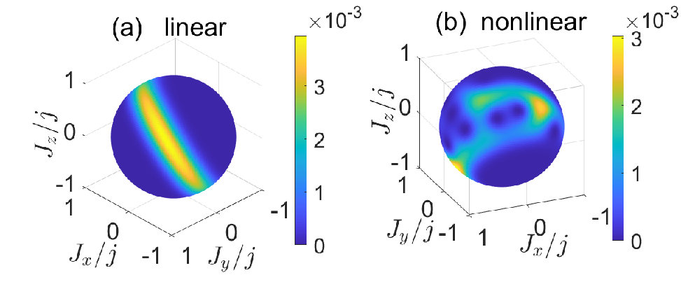
The state distribution can be also illustrated by the Husimi Q function, which represents the anisotropic quasiprobability distribution in a spherical phase space. The Q function is defined as WA; JM

\displaystyle Q(\theta_{0},\phi_{0})=\frac{1}{\pi}\langle\theta_{0},\phi_{0}|\rho|\theta_{0},\phi_{0}\rangle,

(24)

where $|\theta_{0},\phi_{0}\rangle$ is the coherent spin state

	$\displaystyle\|\theta_{0},\phi_{0}\rangle=\exp\{i\theta_{0}[J_{x}\sin(\phi_{0})-J_{y}\cos(\phi_{0})]\}\|j,-j\rangle$
			(25)

and $\rho$ is the density matrix of the considered system. In Figs. 4(a) and 4(b), we plot Q functions for the linear and nonlinear scheme, respectively. Compared with the linear scheme, the central area for the nonlinear one [here the nonlinearity strength is $20$ times larger than that in Figs. 3 (b) and (d)] becomes much smaller. Combining the scale of the color bar, we can see that the Q function distribution becomes more uniform for the nonlinear setup. Meanwhile, we plot $|\langle j,m|\psi(t)\rangle|^{2}$ versus $m$ under the same condition (the few number of photons and the relatively big nonlinear effect) in Fig. 4(c) and 4(d). In this case, the compressibility of state distribution for nonlinear scheme are revealed again.

IV conclusion

In conclusion, with reference to the traditional SU(2) interferometer model, we implement a similar algebraic setup for the rotation sensing in a microcavity. In our scheme, we employ a detuning two-level atom to create the effective coupling between two optical modes, thanks to which the initial state is extended to the entire Hilbert space during the time evolution. We find that the accuracy of parameter estimation can be enhanced dramatically by the coupling, via encoding the estimated angular velocity into both of the amplitudes and the phase of the wave function. Moreover, we study the nonlinear system which can be described by the Bose-Hubbard model and find that the accuracy of parameter estimation can even break the Heisenberg limit with the large photon number. This enhancement is associated with the compressibility of state distribution.

Our study suggests some viable strategies that may be used to benefit the enhancement of the rotating sensing which include as following: use a large-detuned atom to induce the coupling between two optical modes; introduce some nonlinear interaction in the system; rotating the system with a certain angular velocity. We hope that our metrology scheme with the assistance of detuning particle can be useful for the designing of quantum gyroscope based on Sagnac effect.

Acknowledgements.

We thank Prof. X.-M. Lu for useful discussions. This work is supported by National Key R

\&

D Program of China (No. 2021YFE0193500), by National Natural Science Foundation of China (Grant No. 11875011, No. 12047566, No. 11875231 and No. 11935012.).

Appendix A Frölich-Nakajima transformation

For our model of the WGM optical microresonator which couples to a two-level detuning atom, the Hamiltonian can be described by Eq. (13) and (14) in the main text. The rotating-wave approximation demands that the coupling strength and detuning satisfy, respectively, $g_{\gamma}\ll\{\omega_{\gamma},\omega_{a}\}$ and $|\Delta_{\gamma}|\ll\{\omega_{\gamma},\omega_{a}\}$ , where $\Delta_{\gamma}=\omega_{a}-\omega_{\gamma}$ .

To proceed, we assume $g_{\gamma}\ll\Delta_{\gamma}$ , the effective coupling between two cavity modes are obtained by the Frölich-Nakajima transformation H. B. Zhu; Y. Li C. Bruder; M. Boissonneault, which is widely used in condensed-matter physics and quantum optics. By eliminating the degree of freedom of the atom, a weak coupling will be established between the two modes. In what follows, we will give the detailed derivations for the transformation.

At first, we introduce a unitary transformation $\tilde{H}=\exp(-\lambda S)H\exp(\lambda S)$ , which can be expanded via Taylor expansions:

	$\displaystyle\tilde{H}$	$\displaystyle\approx$	$\displaystyle H_{0}+\lambda(H_{I}+[H_{0},S])$
		$\displaystyle+$	$\displaystyle\lambda^{2}([H_{I},S]+[S,[S,H_{0}]])+O(\lambda),$

where $\lambda$ is introduced to mark the order of perturbation and would be set to 1 after all calculations. $S$ is an anti-Hermitian operator. Then, setting the first-order perturbation term $H_{I}+[H_{0},S]=0$ , we obtain

\displaystyle S=g_{\rm cw}a_{\rm cw}|e\rangle\langle g|+g_{\rm ccw}a_{\rm ccw}|e\rangle\langle g|-\rm{H.c}.

(27)

Considering the dispersive interaction between the atom and resonator modes, we approximate that the atom prepared in initial state $|g\rangle$ will always be in the ground state $|g\rangle$ . Neglecting the high-frequency terms, the effective Hamiltonian satisfies

\displaystyle\tilde{H}

\displaystyle=

\displaystyle H_{\rm eff}\otimes|g\rangle\langle g|.

(28)

At last, up to second order interactions, our effective Hamiltonian is obtained as $H_{\rm eff}=H_{\rm eff,\omega}+H_{{\rm eff},I}$ , where

\displaystyle H_{\rm eff,\omega}=\sum_{\gamma}\left(\omega_{\gamma+}\frac{|g_{\gamma}|^{2}}{\Delta_{\gamma}}\right)a_{\gamma}^{\dagger}a_{\gamma},

(29)

and

\displaystyle H_{{\rm eff},I}=\sum_{\gamma,\gamma^{\prime}\neq\gamma}\frac{1}{2}(\frac{1}{\Delta_{\gamma}}+\frac{1}{\Delta_{\gamma^{\prime}}})g_{\gamma}g_{\gamma^{\prime}}a_{\gamma}^{\dagger}a_{\gamma^{\prime}}.

(30)

We further define

\displaystyle g_{\rm eff}=\frac{1}{2}\left(\frac{1}{\Delta_{\rm cw}}+\frac{1}{\Delta_{\rm ccw}}\right)g_{\rm cw}g_{\rm ccw},

(31)

in the interaction picture and Schwinger representation, the effective Hamiltonian can be reduced

	$\displaystyle\tilde{H}_{\rm eff}$	$\displaystyle=$	$\displaystyle\exp(iH_{{\rm eff},\omega}t)H_{{\rm eff},I}\exp(-iH_{{\rm eff},\omega}t)$		(32)
		$\displaystyle=$	$\displaystyle 2\Delta J_{z}+2g_{\rm eff}J_{x}.$		(32)

which is Eq. (15) in the main text.

To verify the above approach, we respectively employ the exact Hamiltonian [see Eq. (13) and (14)] and the approximate Hamiltonian $\tilde{H}_{\rm eff}$ to illustrate the dynamics of system. Choosing the initial state as $|in\rangle=(|n,n,g\rangle+|n+1,n-1,g\rangle)/\sqrt{2}$ and $|in\rangle=(|n,n\rangle+|n+1,n-1\rangle)/\sqrt{2}$ for exact and approximate approaches respectively. We compare the dynamics of of the system in Fig. 5. Here, we plot the dynamics of $P_{\rm exac}=|\langle n,n|\psi_{\rm exac}(t)\rangle|^{2}$ (the blue dotted line) and the detuning atom $P_{a}=|\langle e|\psi_{\rm exac}(t)\rangle|^{2}$ (the black dotted line) for the exact solution. Moreover, for the approximate solution, we plot the dynamics of $P_{\rm appr}=|\langle n,n|\psi_{\rm appr}(t)\rangle|^{2}$ (the red solid line). The agreement between $P_{\rm exac}$ and $P_{\rm appr}$ shows the validity of our approach. And the fact $P_{a}\approx 0$ during the time evolution gives a numerical verification of the Eq. (28).

Appendix B QFI in different state

In the main text, we have mentioned that the QFI is enhanced by encoding the parameter $\Delta$ into both of the amplitudes and the phase of the wave function. We will give more details in this appendix. To this end, we now define a general pure state

\displaystyle|\psi\rangle

\displaystyle=

\displaystyle\sum_{n}a_{n}\exp\left(i\varphi_{n}\right)|\psi_{n}\rangle.

(33)

where $\varphi_{n}$ and $a_{n}$ are the real phase and the amplitude of the state $|\psi_{n}\rangle$ , respectively, and the normalization condition demands $\sum_{n}a_{n}^{2}=1$ . To analyze the QFI in different state, we consider the following two situations.

First, we consider the case that only the phases are dependent on the estimated parameter, that is $\varphi_{n}=\varphi_{n}(\Delta)$ . Then the QFI is

\displaystyle\mathcal{F}_{1,\Delta}=4\left[\sum_{n}a_{n}^{2}\left(\frac{\partial\varphi_{n}}{\partial\Delta}\right)^{2}-\mid\sum_{n}a_{n}^{2}\frac{\partial\varphi_{n}}{\partial\Delta}\mid^{2}\right].

(34)

Second, when the phases and the probability amplitudes are both related to $\Delta$ , the QFI can be obtained by

\displaystyle\mathcal{F}_{2,\Delta}=\mathcal{F}_{1,\Delta}+4\sum_{n}\left(\frac{\partial a_{n}}{\partial\Delta}\right)^{2}.

(35)

Here, the second term $4\sum_{n}\left(\frac{\partial a_{n}}{\partial\Delta}\right)^{2}$ is the contribution from the probability amplitudes with parameter $\Delta$ . Obviously, encoding the information of $\Delta$ into both of the phases and the amplitudes is beneficial for parameter estimation.

Appendix C QFI for nonlinear effect

In the Eq. (23) of the main text, we have obtained the formal solution of the Hermitian operator $\mathcal{H}$ . Here, we give the concrete expression and derivation process through the Baker-Hausdoff formula S. S. Pang; J. Liu; X. X. Jing:

\displaystyle\mathcal{H}=-t\frac{\partial H}{\partial\Delta}+i\sum_{n=1}^{\infty}\frac{(it)^{n+1}}{(n+1)!}H^{\times n}\frac{\partial H}{\partial\Delta}

(36)

where the super operator $H^{\times n}$ denotes a $n$ th-order nested commutator operation, $H^{\times}(\cdot)=[H,\cdot]$ . Then we have

$\displaystyle\mathcal{H}$	$\displaystyle=$	$\displaystyle C_{x}J_{x}+C_{y}J_{y}+C_{z}J_{z}+C_{xx}(J_{x}^{2}-J_{y}^{2})$	(37)
		$\displaystyle+C_{yy}(J_{y}^{2}-J_{z}^{2})+C_{xy}(J_{x}J_{y}+J_{y}J_{x})$
		$\displaystyle+C_{yz}(J_{y}J_{z}+J_{z}J_{y})+C_{zx}(J_{z}J_{x}+J_{x}J_{z}),$

where

$\displaystyle C_{xy}$	$\displaystyle=$	$\displaystyle-\frac{e}{6f^{2}}\frac{\partial f}{\partial\Delta}\{\frac{2A_{1}}{r^{2}}[\cos(rt)-1]$	(38)
	$\displaystyle-$	$\displaystyle\frac{A_{1}-B_{1}/\eta}{\Lambda_{1}^{2}}[\cos(\Lambda_{1}t)-1]$
	$\displaystyle-$	$\displaystyle\frac{A_{1}+B_{1}/\eta}{\Lambda_{2}^{2}}[\cos(\Lambda_{2}t)-1]\},$

$\displaystyle C_{yz}$	$\displaystyle=$	$\displaystyle\frac{e}{3fd}\frac{\partial f}{\partial\Delta}\{\frac{A_{2}}{r^{2}}[\cos(rt)-1]$	(39)
	$\displaystyle-$	$\displaystyle\frac{A_{2}+B_{2}/\eta}{2\Lambda_{1}^{3}}[\cos(\Lambda_{1}t)-1]$
	$\displaystyle-$	$\displaystyle\frac{A_{2}-B_{2}/\eta}{2\Lambda_{2}^{3}}[\cos(\Lambda_{2}t)-1]\},$

$\displaystyle C_{zx}$	$\displaystyle=$	$\displaystyle\frac{e}{3f^{2}d}\frac{\partial f}{\partial\Delta}\{\frac{A_{3}+f^{2}d^{2}}{r^{3}}[\sin(rt)-rt]$	(40)
	$\displaystyle-$	$\displaystyle\frac{A_{3}+B_{3}/\eta}{2\Lambda_{1}^{3}}[\sin(\Lambda_{1}t)-\Lambda_{1}t]$
	$\displaystyle-$	$\displaystyle\frac{A_{3}-B_{3}/\eta}{2\Lambda_{2}^{3}}[\sin(\Lambda_{2}t)-\Lambda_{2}t]\},$

$\displaystyle C_{xx}$	$\displaystyle=$	$\displaystyle-\frac{e}{6f}\frac{\partial f}{\partial\Delta}\{\frac{2A_{1}}{r^{3}}[\sin(rt)-rt]$	(41)
	$\displaystyle-$	$\displaystyle\frac{A_{1}-B_{1}/\eta}{\Lambda_{1}^{3}}[\sin(\Lambda_{1}t)-\Lambda_{1}t]$
	$\displaystyle-$	$\displaystyle\frac{A_{1}+B_{1}/\eta}{\Lambda_{2}^{3}}[\sin(\Lambda_{2}t)-\Lambda_{2}t]\},$

and

$\displaystyle C_{yy}$	$\displaystyle=$	$\displaystyle\frac{e}{3f}\frac{\partial f}{\partial\Delta}\{\frac{2A_{2}}{r^{3}}[\sin(rt)-rt]$	(42)
	$\displaystyle-$	$\displaystyle\frac{A_{2}+B_{2}/\eta}{\Lambda_{1}^{3}}[\sin(\Lambda_{1}t)-\Lambda_{1}t]$
	$\displaystyle-$	$\displaystyle\frac{A_{2}-B_{2}/\eta}{\Lambda_{2}^{3}}[\sin(\Lambda_{2}t)-\Lambda_{2}t]\}.$

where $\Lambda_{1}=[(3f^{2}+3d^{2}-\eta)/2]^{1/2}$ , $\Lambda_{2}=[(3f^{2}+3d^{2}+\eta)/2]^{1/2}$ , $\eta=[f^{4}+d^{4}+14f^{2}d^{2}]^{1/2}$ and

\displaystyle\begin{cases}A_{1}=d^{2}-4f^{2}&B_{1}=(f^{2}-d^{2})(4f^{2}+d^{2})\\ A_{2}=f^{2}-d^{2}&B_{2}=f^{4}-d^{4}+6f^{2}d^{2}\\ A_{3}=2f^{4}+d^{4}-6f^{2}d^{2}&B_{3}=2f^{6}+d^{6}+8f^{4}d^{2}+f^{2}d^{4}.\\ \end{cases}

The complete expression for the QFI $\mathcal{F}_{\Delta}=4(\langle\mathcal{H}^{2}\rangle-\langle\mathcal{H}\rangle^{2})$ [with $\mathcal{H}$ being given by Eq. (23)] possesses $36$ terms, which is too tedious to be given term by term here. However, we note that $\{C_{xx},C_{yy},C_{xy},C_{yz},C_{zx}\}\propto e^{1}$ and $\{C_{x},C_{y},C_{z}\}\propto e^{0}$ . Therefore, in the expression of the QFI, $6$ terms are proportional to $e^{0}$ , $15$ terms are proportional to $e^{1}$ while the remaining $15$ terms are proportional to $e^{2}$ . The first $6$ terms in the order of $e^{0}$ are exactly the QFI without the nonlinear interaction, which is given by Eq. (19) in the main text. The last $15$ terms in the order of $e^{2}$ can be neglected in the situation of small $e$ . Now, we give one typical term which is proportional to $e^{1}$ , for example

			$\displaystyle C_{x}C_{xx}\{\langle J_{x}(J_{x}^{2}-J_{y}^{2})+(J_{x}^{2}-J_{y}^{2})J_{x}\rangle-2\langle J_{x}\rangle\langle J_{x}^{2}-J_{y}^{2}\rangle\}$		(43)
		$\displaystyle\propto$	$\displaystyle\frac{1}{8}C_{x}C_{xx}[(j-1)(j+2)\sqrt{j(j+1)}].$		(43)

Since $j=n/2$ , it shows that we here achieve a $n^{3}$ scaling for the QFI, which is beyond the Heisenberg limit.

References

(1) C. M. Caves, Phys. Rev. Lett. 45, 75 (1980).
(2) C. M. Caves, Phys. Rev. D 23, 1693 (1981).
(3) V. Giovannetti, S. Lloyd and L. Naccone, Science 306, 1330 (2004).
(4) V. Giovannetti, S. Lloyd and L. Naccone, Phys. Rev. Lett. 96, 010401 (2006).
(5) D. W. Berry, B. L. Higgins, S. D. Bartlett, M. W. Mitchell, G. J. Pryde and H. M. Wiseman, Phys. Rev. A 80, 052114 (2006).
(6) J. Joo, W. J. Munro and T. P. Spiller, Phys. Rev. Lett. 107, 083601 (2011).
(7) H. S. Eisenberg, J. F. Hodelin, G. Khoury and D. Bouwmeester, Phys. Rev. Lett. 94, 090502 (2005).
(8) I. Afek, O. Amber and Y. Silberberg, Science 328, 879 (2010).
(9) K. J. Resch, K. L. Rregnell, R. Prevedel, A. Gilchrist, G. J. Pryde, J. L. O’Brien and A. G. White. Phys. Rev. Lett. 98, 223601 (2007).
(10) D. Leibfried, M. D. Barrett, T. Schaetz, J. Britton, J. Chiaverini, W. M. Itano, J. D. Jost, C. Langer and D. J. Wineland, Science 304, 1476 (2004).
(11) K. X. Sun, M. M. Fejer, E. Gustafson and R. L. Byer, Phys. Rev. Lett. 76, 3053 (1996).
(12) A. N. Boto, P. Kok, D. S. Abrams, S. L. Braunstein, C. P. Williams and J. P. Dowling, Phys. Rev. Lett. 85, 2733 (2000).
(13) S. J. Bentley and R. W. Boyd, Opt. Express 12, 5735 (2004).
(14) S. H. Tan, B. I. Erkmen, V. Giovannetti, S. Guha, S. Lloyd, L. Maccone, S. Pirandola and J. H. Shapiro, Phys. Rev. Lett. 101, 253601 (2008).
(15) V. Giovannetti, S. Lloyd, L. Maccone and J. H. Shapiro, Phys. Rev. A 79, 013827 (2009).
(16) M. Tsang, J. H. Shapiro and S. Lloyd, Phys. Rev.A 78, 053820 (2008).
(17) S. Lloyd, Science 321, 1463 (2008).
(18) G. Khoury, H. S. Eisenberg, E. J. S. Fonseca, and D. Bouwmeester, Phys. Rev. Lett. 98, 203601 (2006).
(19) S. D. Huver, C. F. Wildfeuer and J. P. Dowling, Phys. Rev. A 78, 063828 (2008).
(20) B. Yurke, S. L. McCall and J. R. Klauder, Phys. Rev. A 33, 4033 (1986).
(21) M. Kasevich and S. Chu, Phys. Rev. Lett. 69, 1741 (1992).
(22) C. E. Wieman, D. E. Pritchard and D. J. Wineland, Rev. Mod. Phys. 71, S253 (1999).
(23) X. M. Lu, H. Krovi, R. Nair, S. Guha and J. H. Shapiro, npj Quantum Inf. 4, 64 (2018).
(24) N. Fang, H. Lee, C. Sun and X. Zhang, Science 308, 534 (2006).
(25) J. G. Fujimoto, M. E. Brezinski, G. J. Tearney, S. A. Boppart, B. Bouma, M. R. Hee, J. F. Southern and E. A. Swanson, Nature Medicine 1, 970 (1995).
(26) Y. Martin, D. W. Abraham and H. K. Wickramasinghe, Appl. Phys. Lett. 52, 1103 (1988).
(27) F. Jelezko and J. Wrachtrup, Phys. Status Solidi A 203, 3207 (2006).
(28) M. W. Doherty, V. V. Struzhkin, D. A. Simpson, L. P. M. Guinness, Y. Meng, A. Stacey, T. J. Karle, R. J. Hemley, N. B. Manson, L. C. L. Hollenberg and S. Prawer, Phys. Rev. Lett. 112, 047601 (2014).
(29) L. Rondin, J. P. Tetienne, T. Hingant, J. F. Roch, P. Maletinsky and V. Jacques, Rep. Prog. Phys. 77, 056503 (2014).
(30) G. Balasubramanian, P. Neumann, D. Twitchen, M. Markham, R. Kolesov, N. Mizuochi, J. Isoya, J. Achard, J. Beck, J. Tissler, V. Jacques, P. R. Hemmer, F. Jelezko and J. Wrachtrup, Nat. Mater. 8, 383 (2009).
(31) T. Wolf, P. Neumann, K. Nakamura, H. Sumiya, T. Ohshima, J. Isoya and J. Wrachtrup, Phys. Rev. X 5,041001 (2015).
(32) K. U. Schreiber and J.-P. R. Wells, Rev. Sci. Instrum. 84, 041101 (2013).
(33) A. D. V. Di Virgilio, A. Basti, N. Beverini, F. Bosi, G. Carelli, D. Ciampini, F. Fuso, U. Giacomelli, E. Maccioni, P. Marsili, A. Ortolan, A. Porzio, A. Simonelli, and G.Terreni, Phys. Rev. Res. 2, 032069(R) (2020).
(34) J. Ahn, Z. Xu, J. Bang, Y.-H. Deng, T. M. Hoang, Q. Han, R.-M. Ma and T. Li, Phys. Rev. Lett. 121, 033603 (2018).
(35) R. Reimann, M. Doderer, E. Hebestreit, R. Diehl, M. Frimmer, D. Windey, F. Tebbenjohanns and L. Novotny, Phys. Rev. Lett. 121, 033602 (2018).
(36) S. L. Braunstein and C. M. Caves, Phys. Rev. Lett. 72, 3439 (1994).
(37) S. L. Braunstein, C. M. Caves and G. J. Milburn, Ann. Phys. NY 247, 135 (1996).
(38) W. W. Chow, J. Gea-Banacloche, L. M. Pedrotti, V. E. Sanders, W. Schleich and M. O. Scully, Rev. Mod. Phys. 57, 61 (1985).
(39) J. Li, M. G. Suh and K. Vahala, Optica 4, 346 (2017).
(40) M. N. Armenise, C. Ciminelli, F. Dell’Olio and V. M. M. Passaro, Advances in Gyroscope Technologies, Springer (2010).
(41) S. Maayani, R. Dahan, Y. Kligerman, E. Moses, A. U. Hassan, H. Jing, F. Nori, D. N. Christodoulides and T. Carmon, Nature 558, 569 (2018).
(42) G. B. Malykin, Phys, Usp. 43, 1229 (2000).
(43) X. X. Jing, J. Liu, H. N. Xiong and X. G. Wang, Phys. Rev. A 92, 012312 (2015).
(44) J. Liu, X. X. Jing and X. G. Wang, Sci. Rep. 5, 8565 (2014).
(45) M. J. Hatmann, F. G. S. L. Brandão and M. B. Plenio, Laser & Photons. Rev. 2, 527 (2008).
(46) M. J. Hatmann, F. G. S. L. Brandão and M. B. Plenio, New J. Phys. 10, 033011 (2008).
(47) L. Pezze and A. Smerzi, Phys. Rev. Lett. 102, 100401 (2009).
(48) J. Beltran and A. Luis, Phys. Rev. A 72, 045801 (2005).
(49) A. Luis, Phys. Lett. A 329, 8 (2005).
(50) A. Widera, S. Trotzky, P. Cheinet, S. Folling, F. Gerbier, I. Bloch, V. Gritsev, M. D. Lukin and E. Demler, Phys. Rev. Lett. 100, 140401 (2008).
(51) J. M. Radcliffe, J. Phys. A 4, 313 (1971).
(52) H. B. Zhu and C. P. Sun, Chin. Sci. A 30, 928 (2000); Prog. Chin. Sci. 10, 698 (2000).
(53) Y. Li, C. Brude and C. P. Sun, Phys. Rev. A 75, 032302 (2007).
(54) M. Boissonneault, J. M. Gambetta and A. Blais, Phys. Rev. A 79, 013819 (2009).
(55) S. S. Pang and T. A. Brun, Phys. Rev. A 90, 022117 (2014).

	$\displaystyle J_{z}\|j,m\rangle$	$\displaystyle=$	$\displaystyle m\|j,m\rangle,$
	$\displaystyle J^{2}\|j,m\rangle$	$\displaystyle=$	$\displaystyle j(j+1)\|j,m\rangle,$		(4)