A context-aware gate set tomography characterization
of superconducting qubitsPreprint: APS/123-QED
Abstract
The efficiency of Quantum Characterisation, Verification, and Validation (QCVV) protocols highly hinges on the agreement between the assumed noise model and the underlying error mechanisms. As a matter of fact, errors in Quantum Processing Units (QPUs) incorporate various aspects of context-dependability which are overlooked by the majority of the commonly used QCVV protocols. As QCVV protocols are indispensable when it comes to characterizing and evaluating quantum operations, there is a serious need for a detailed characterization taking into account such aspects. In this work, we address these shortcomings by designing a context-aware version of the gate set tomography (GST) protocol. Our experiment selection approach is based on a polynomial quantification of the accumulation of errors within the designed circuits. Using simulated QPUs, we show that this technique enables a characterization with an inaccuracy reaching . Furthermore, we use our proposed protocol to experimentally infer context-dependent errors, namely crosstalk and memory effects, in a publicly accessible cloud-based superconducting qubits platform. Our results show that when the GST is upgraded to include such features of context-awareness, a large coherence in the errors is observed. These findings open up possibilities of drastically reducing the errors within the currently demonstrated QPUs.
I Introduction
A quantum state is by essence destructed when measured Nielsen and Chuang 2010. Therefore, real-time monitoring of the computational states of QPUs while preserving their quantum aspect is generally unlikely. In combination with being subject to numerous noise mechanisms, this fact implies that the creation of quantum states and the different operations applied to them can only be evaluated indirectly. In quantum computing, these practices are commonly known as QCVV protocols. They consist of sampling sequences of operations and converting the observed measurements into meaningful parameters. Designing efficient QCVV protocols is a major challenge in this field, as they are vital for understanding noise mechanisms Dehollain et al. 2016; Erhard et al. 2019, calibrating control signals Reed 2013; Watson et al. 2018, developing noise-aware compilers Murali et al. 2020, and providing realistic noise models for simulation backends Moueddene et al. 2020.
There exist a wide range of QCVV protocols designed for targeting a variety of noise mechanisms Sarovar et al. 2020; Helsen et al. 2019; Nielsen et al. 2020a; Leibfried et al. 1996; Paris and Řeháček 2004; James et al. 2001; Artiles et al. 2005; Chuang and Nielsen 1997; Xin et al. 2019; Knill et al. 2008; Wood and Gambetta 2018; McKay et al. 2020; Palmieri et al. 2020; Govia et al. 2020; Blume-Kohout et al. 2013; Greenbaum 2015; Blume-Kohout et al. 2017; Nielsen et al. 2020b; Erhard et al. 2019. These protocols exhibit an interplay between the number of extracted parameters, the expected accuracy, the number of the measured sequences, and the awareness of systematic errors. For instance, Randomized Benchmarking (RB) protocol is used to infer the depolarizing rate of quantum gates Knill et al. 2008. This protocol owes its high accuracy to its output corresponding to a single parameter (the error rate) and its awareness to State Preparation And Measurement (SPAM) errors. other examples are quantum state tomography Pauli 1980; Leibfried et al. 1996; Paris and Řeháček 2004; James et al. 2001 and quantum process tomography Artiles et al. 2005; Chuang and Nielsen 1997. They are used to respectively infer quantum states and quantum operations. These protocols provide a more detailed characterization as their outputs are density matrices and quantum channels. However, unless properly addressed Palmieri et al. 2020; Govia et al. 2020, their standard forms have moderate accuracy, as they are oblivious to systematic errors and based on sampling a relatively small number of sequences. As an alternative, the Gate Set Tomography (GST) protocol provides a more accurate and detailed characterization since it takes into account and evaluates SPAM errors and relies on sampling a larger number of sequences Blume-Kohout et al. 2013; Greenbaum 2015; Blume-Kohout et al. 2017; Nielsen et al. 2020b. Although the requirement of measuring a large number of sequences comes with a high time complexity (fridge time), it was demonstrated that involving the GST protocol in the calibration routines leads to a considerable reduction in the underlying operational errors Dehollain et al. 2016; White et al. 2021. In other works, data delivered by measuring the GST sequences were used to infer deliberately engineered temporally correlated noise processes Mavadia et al. 2018 and context-dependent errors Rudinger et al. 2019; Proctor et al. 2020. However, the state of the art suffers from the lack of GST protocols adapted to capturing sophisticated forms of errors, namely crosstalk in large arrays of qubits(beyond three qubits) and memory effects. These noise mechanisms were not captured by the original GST protocol
To characterize crosstalk errors in a set of qubits; how a given operation on a target qubit is affected given the operations simultaneously applied to the neighboring qubits, one can conceive two approaches involving the context agnostic GST. The first one is to perform a multiqubit GST on the whole set then trace out the neighboring qubits. This approach is impractical as the operators describing multiqubit gates are massive for sets containing more than 2 qubits. The second alternative is to perform multiple rounds of single-qubit GST on the target qubit. In each round, the target gates are accompanied by a different configuration of gates on the neighboring qubit which enables inferring crosstalk. In this paper, we introduce a context-aware version of the GST protocol. It systematically takes into account spatial correlations which allows inferring the target operations in a multiplicity of scenarios within a single round. Therefore, it reduces considerably the time complexity that comes with the requirement of running multiple rounds of the latter approach while it tackles the impracticality of the first one. Additionally, it also takes into account spatial correlations which allows characterizing memory effects. Therefore, the proposed protocol is a step towards enabling a rigorous assessment of the erroneous behavior of QPUs. In short, the main contributions of this paper are:
- •
The development and the validation of a new version of the GST protocol based on the refinement of the sequence selection algorithm, allowing a high error characterization accuracy.
- •
The differentiation of the proposed version by introducing the context-awareness, enabling the characterization of crosstalk errors and memory effects.
- •
The demonstration of the protocol on Quantum-Inspire’s Starmon-5 chip QuTech 2018; the results reveal a relevant context-dependency in the error mechanisms affecting this chip with considerably large reversible parts.
Suppose one possesses a QPU offering the possibility to run a target gate set composed of state preparation, a set of gates , and a measurement. We assume these operations are governed by a noise mechanism such that each one of these operations corresponds to a well-known operator/superoperator;i.e., state preparation, ith-quantum gate and the measurement respectively corresponds to a state , a quantum channel and a measurement operator . Therefore, as we know these operators, we can compute the expectation values of any circuit built as a combination with repetition of elements of this gate set. For instance, the measurement applied to a circuit defined by state preparation followed by a sequence of length of gates is predicted to generate the following expectation values:
| (1) |
Let’s put ourselves in the inverse case where , and are unknown and we are given the possibility of sampling a set of N circuits with corresponding sequences where . The claim of the GST protocol is that the operators , and can be estimated based on the observed measurements Blume-Kohout et al. 2017; Greenbaum 2015. In other words, if the measurement of the circuits on the target QPU generated measurements , the gate set , and is inferred by constructing a set of operations generating similar measurements values. This reconstruction is equivalent to the following optimization problem:
Given: a set of circuits and the corresponding average of observed measurements on target QPU:
minimize the following L1 loss function:
| (2) |
where refers to the absolute value. This optimization is identified as a Total Variation Diminishing (TVD) problem whom the freedom degrees are the nontrivial elements of the operators describing the gate set. The fact that the gates are quantum maps together with the Hermicity and the unit trace of density matrices and measurement operators imply the following linear constraints on their entries):
| (3) | |||||
The starting point in our optimizations is the operators corresponding to the perfect target operations (no errors). As there is gauge freedom in these operators Łukasz Rudnicki et al. 2017, one should ensure that the estimations are close to the perfect operations. Therefore, we intuitively tighten these linear constraints around the perfect operation with a marge of for gates and for SPAM operators, and hence, given the perfect operations , and , These constraints become:
| (4) | |||||
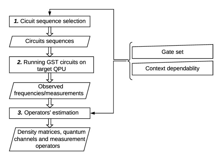
Furthermore, the GST relies on sampling a large number of circuit sequences to provide an accurate characterization of the operations within a target QPU. However, sampling any set of circuits sequence does not ensure an accurate characterization. In fact, gate errors can either add up or cancel out. The latter case leads to the insensitivity of the observed measurement to error parameters, and hence, alters the accuracy of the protocol. Therefore, as displayed in Figure 1, the first step of the GST protocol, introduced in the supplementary material, is to design a set of sequences that guarantees the full imaging of the core sequences and the amplification of the manifestations of the targeted errors as these sequences’ length increases. The second step consists of running multiple shots of the circuits designed in step 1 on the target QPU and collecting the observed measurements. Finally, the third step, as we just described in this section, is to estimate the operators describing the gate set using the observed measurements in step 2.
In the next sections, We describe the adaptation of this protocol;i.e. the introduction of context-awareness, to infer temporal and spatial correlation in superconducting qubits and report our findings. Note that we consider it convenient to focus on errors affecting idling gates. This convenience comes from the fact that the impact of the investigated noise mechanisms is better observed/understood when affecting idling errors. Also, the accuracy of the GST protocol characterization of idling gates is very high compared to operational errors. The latter is altered by the gauge equivalence of quantum channels Łukasz Rudnicki et al. 2017 and remain a challenge that we don’t address in depth in this work,
II Crosstalk evaluation

A quantum operation on a set of qubits may induce errors to operations simultaneously applied to neighboring qubits via crosstalk effects. In current superconducting qubits, crosstalk is prominent when C-phase gates are in play McKay et al. 2020. If we look at the geometry of a Starmon-5 chip in Figure 2, we see that qubit Q1 is physically connected to Q2. Also, when a single qubit gate is applied to Q1, Q2 can undergo three different C-phases with Q0, Q3, or Q4. The goal of this subsection is to use the GST protocol to characterize the impact of these C-phases on the operations simultaneously applied to Q1. To do so, we assume that depending on the operations applied to the rest of the qubits of the chip, a quantum gate, say an idling gate , can be described by multiple superoperators . Each superoperator is specific to a context that is defined by the operations applied to the rest of the qubits of the chips. We include contexts that corresponds respectively to Q2 undergoing C-phases with Q0, Q3, and Q4 (while the two qubits left are idling) and a reference context where all the qubits are idling. Furthermore, to achieve informational completeness, we enable the possibility of including ancillary and rotations on Q1 in the context in our circuits. However, as our main goal is to infer idling gates, these ancillary operations’ corresponding error generators are discarded from matrix in the germs selection algorithm. Using the genetic algorithm from the MatLab optimization toolbox, the latter provides the following set of germs:
| (5) | |||||
Note that the upper index refers to the context For instance, respectively describe the idling operations on Q1 that is accompanied by Cphases on Q2 together with respectively Q0, Q3, Q4 while the rest of the qubits is idling. Therefore, each of these operations are captured by running 5-qubits gates . Since C-phases in the Starmon-5 are implemented within three times the duration of single-qubit gates, to every single-qubit gate is appended an idling time to ensure the parallelism within the elements of the gate set. Our characterization yields the following Pauli superoperators:
| (6) |
| (7) |
| (8) |
| (9) |
These operators’ respective diamond distances to the target perfect operators (no errors) are 0.0160, 0.0218, 0.0210, and 0.0083. The diamond distance is computed using QETLAB Johnston 2016 and The CVX-package Grant and Boyd 2014; Grant and Boyd 2008. Furthermore, this characterization allows us to study more features of this noise mechanism. For instance, due to the apparent anti-symmetry of the unital block with respect to the diagonal, we see a clear resemblance of these matrices to elements of the (the group of -rotations). An idling gate that displays such a feature of noise would imply that this form of noise is coherent, and hence, avoidable by inversion. To address this hypothesis, we seek for each operation an unitary operator that minimises . Finding is an optimization problem in which the freedom degrees are the 3 angles that specify . By solving these problems using the SQP algorithm from the Matlab optimization toolbox, we find that for scenarios 1, 2, and 3 it drops to 0.0134, 0.0148, and 0.0119. while there is no apparent improvement in context 4;i.e. .
III Memory effects
In this section, we address the situation where gate errors are accompanied by an error mechanism that lasts slightly longer than the implementation time of the gates themselves. In this case, we say that the environment has a first-order memory:i.e., it alters the current gate differently depending on the previous operation. Therefore, we suppose that each gate is described by multiple superoperators. Each of these superoperators corresponds to a different context that is defined by the previous operation. Suppose we are targeting a gate set composed of an , an , and an idling gate, . If such memory effects are displayed, each one of these gates has three corresponding superoperators. see Table 1.
This configuration leads to constraints on the possible circuits. In fact, in order to be valid, a sequence should satisfy:
| (10) |
These constraints are injected into the germs selection algorithm and the sequences are built accordingly. As we are inferring how memory effects are affecting idling gates, the six gates to are introduced as ancillary gates, and the errors in , and are targeted by our germs selection algorithm. Using the genetic algorithm from the MatLab’s optimization toolbox, our germs selection algorithm provides the following set:
| (11) | |||||

where f is defined by the fiducial sequence’s last gate. We also merge every state initialization with a consecutive idling gate to ensure that the context of the first gate is always 3 (preceded by an idling gate). We also include another idling gate before the final measurement so the latter is operated only in the context (the measurement is not merged with the idling gate). Figure 3 displays a circuit example. We run this designed sequence on qubit Q1 of a Starmon-5. The estimated superoperators of the three Idling gates are:
| (12) |
| (13) |
| (14) |
where corresponds to the idling operator injected at the context that is defined by the previous gate (, , and refers to operations preceded by respectively , , and ). These gates’ diamond distances to the ideal gates are 0.0186, 0.0265 and 0.0057. Seeking and injecting unitaries s that minimise the distances allow to respectively reduce them to 0.0156, 0.0174 and 0.0057.
IV Discussion and outlook
This paper introduces a context-aware version of the GST protocol;i.e., It has the ability to distinguish operations with respect to their context. This adaptation leads to a sharp characterization of errors when they incorporate such context dependencies. To do so, we described the core of our version that consists of a polynomial evaluation of the quality of the circuit sequences. As these evaluation functions admit a polynomial representation, they are computed efficiently. In fact, the fitness function of the germs selection algorithms used in this work take no more than in a single core of a cluster node with 2 Xeon E5-2683 v3 CPUs (@ 2.00GHz = 28 cores / 56 threads) and 24 x 16GB DDR4 = 384GB memory. Furthermore, we evaluate the accuracy of our estimations by using simulated QPUs that fit the assumed model. This evaluation shows that our estimation is two orders of magnitudes more accurate than the gate themselves. Moreover, we adapt the GST protocol to take into account and infer spatial correlations;i.e. crosstalk errors. The implementation of the designed protocol on the Starmon-5 chip shows that when a C-phase is applied to neighboring qubits, errors are induced to the studied qubits via crosstalk. Fortunately, a large fraction of these errors is reversible. For instance, of the errors in Q1’s idling when a C-phase is applied to qubits Q2 and Q4 are coherent. This offers the opportunity of drastically mitigating the errors that are purely due to crosstalk;i.e. in this example a reduction reaching a factor of is predicted. Next, we addressed the problem of temporal correlation, namely memory effects. This study explicitly shows that when an idling gate is applied after a rotation gate, errors due to memory effects are induced. However, up to of these errors is reversible which constitutes a reduction of the errors purely due to memory effects by a factor of . Note that measuring the sequences for these characterizations (designed for a maximal repetition index 6) took respectively and hours for the crosstalk and memory effects experiments.
To conclude, this work takes a step further the agreement between the assumed noise model by GST protocol and real-life error mechanisms. However, the efficiency of the hereby proposed Context-Aware GST (CA-GST) protocol is altered by sampling errors and the presence of errors mechanisms that reside beyond the assumed models. Nevertheless, due to their hereby demonstrated coherent aspect, this work promises a large reduction in some of the most prominent error mechanisms in this era.
Acknowledgements.
The authors would like to thank Diogo Valada, and Hans van Someren for their technical support and Miguel Moreira for describing to us the operations on Quantum-Inspires’s Starmon-5 chip. The authors would like to acknowledge funding from Intel Corporation.References
- Nielsen and Chuang (2010) M. A. Nielsen and I. L. Chuang, Quantum Computation and Quantum Information (Cambridge University Press, Massachusetts Institute of Technology, 2010).
- Dehollain et al. (2016) J. P. Dehollain, J. T. Muhonen, R. Blume-Kohout, K. M. Rudinger, J. K. Gamble, E. Nielsen, A. Laucht, S. Simmons, R. Kalra, A. S. Dzurak, and A. Morello, Optimization of a solid-state electron spin qubit using gate set tomography, New Journal of Physics 18, 103018 (2016).
- Erhard et al. (2019) A. Erhard, J. J. Wallman, L. Postler, M. Meth, R. Stricker, E. A. Martinez, P. Schindler, T. Monz, J. Emerson, R. Blatt, and et al., Characterizing large-scale quantum computers via cycle benchmarking, Nature Communications 10, 10.1038/s41467-019-13068-7 (2019).
- Reed (2013) M. Reed, Entanglement and quantum error correction with superconducting qubits (2013), arXiv:1311.6759 .
- Watson et al. (2018) T. F. Watson, S. G. J. Philips, E. Kawakami, D. R. Ward, P. Scarlino, M. Veldhorst, D. E. Savage, M. G. Lagally, M. Friesen, S. N. Coppersmith, M. A. Eriksson, and L. M. K. Vandersypen, A programmable two-qubit quantum processor in silicon, Nature 555, 633 (2018).
- Murali et al. (2020) P. Murali, D. C. Mckay, M. Martonosi, and A. Javadi-Abhari, Software mitigation of crosstalk on noisy intermediate-scale quantum computers, in Proceedings of the Twenty-Fifth International Conference on Architectural Support for Programming Languages and Operating Systems (ACM, 2020).
- Moueddene et al. (2020) A. A. Moueddene, N. Khammassi, K. Bertels, and C. G. Almudever, Realistic simulation of quantum computation using unitary and measurement channels, Phys. Rev. A 102, 052608 (2020).
- Sarovar et al. (2020) M. Sarovar, T. Proctor, K. Rudinger, K. Young, E. Nielsen, and R. Blume-Kohout, Detecting crosstalk errors in quantum information processors, Quantum 4, 321 (2020).
- Helsen et al. (2019) J. Helsen, F. Battistel, and B. M. Terhal, Spectral quantum tomography, npj Quantum Information 5, 10.1038/s41534-019-0189-0 (2019).
- Nielsen et al. (2020a) E. Nielsen, K. Rudinger, T. Proctor, A. Russo, K. Young, and R. Blume-Kohout, Probing quantum processor performance with pygsti 10.1088/2058-9565/ab8aa4 (2020a), arXiv:2002.12476 .
- Leibfried et al. (1996) D. Leibfried, D. M. Meekhof, B. E. King, C. Monroe, W. M. Itano, and D. J. Wineland, Experimental determination of the motional quantum state of a trapped atom, Phys. Rev. Lett. 77, 4281 (1996).
- Paris and Řeháček (2004) M. Paris and J. Řeháček, Quantum State Estimation (Springer, Berlin, Heidelberg, 2004).
- James et al. (2001) D. F. V. James, P. G. Kwiat, W. J. Munro, and A. G. White, Measurement of qubits, Phys. Rev. A 64, 052312 (2001).
- Artiles et al. (2005) L. Artiles, R. D. Gill, and M. Guta, An invitation to quantum tomography, Journal of the Royal Statistical Society Series B 67, 109 (2005).
- Chuang and Nielsen (1997) I. L. Chuang and M. A. Nielsen, Prescription for experimental determination of the dynamics of a quantum black box, Journal of Modern Optics 44, 2455 (1997).
- Xin et al. (2019) T. Xin, S. Lu, N. Cao, G. Anikeeva, D. Lu, J. Li, G. Long, and B. Zeng, Local-measurement-based quantum state tomography via neural networks, npj Quantum Information 5, 10.1038/s41534-019-0222-3 (2019).
- Knill et al. (2008) E. Knill, D. Leibfried, R. Reichle, J. Britton, R. B. Blakestad, J. D. Jost, C. Langer, R. Ozeri, S. Seidelin, and D. J. Wineland, Randomized benchmarking of quantum gates, Phys. Rev. A 77, 012307 (2008).
- Wood and Gambetta (2018) C. J. Wood and J. M. Gambetta, Quantification and characterization of leakage errors, Phys. Rev. A 97, 032306 (2018).
- McKay et al. (2020) D. C. McKay, A. W. Cross, C. J. Wood, and J. M. Gambetta, Correlated randomized benchmarking (2020), arXiv:2003.02354 .
- Palmieri et al. (2020) A. M. Palmieri, E. Kovlakov, F. Bianchi, D. Yudin, S. Straupe, J. D. Biamonte, and S. Kulik, Experimental neural network enhanced quantum tomography, npj Quantum Information 6, 10.1038/s41534-020-0248-6 (2020).
- Govia et al. (2020) L. C. G. Govia, G. J. Ribeill, D. Ristè, M. Ware, and H. Krovi, Bootstrapping quantum process tomography via a perturbative ansatz, Nature Communications 11, 10.1038/s41467-020-14873-1 (2020).
- Blume-Kohout et al. (2013) R. Blume-Kohout, J. K. Gamble, E. Nielsen, J. Mizrahi, J. D. Sterk, and P. Maunz, Robust, self-consistent, closed-form tomography of quantum logic gates on a trapped ion qubit (2013), arXiv:1310.4492 .
- Greenbaum (2015) D. Greenbaum, Introduction to quantum gate set tomography, 67 (2015).
- Blume-Kohout et al. (2017) R. Blume-Kohout, J. K. Gamble, E. Nielsen, K. Rudinger, J. Mizrahi, K. Fortier, and P. Maunz, Demonstration of qubit operations below a rigorous fault tolerance threshold with gate set tomography, nature communications 8, https://doi.org/10.1038/ncomms14485 (2017).
- Nielsen et al. (2020b) E. Nielsen, J. K. Gamble, K. Rudinger, T. Scholten, K. Young, and R. Blume-Kohout, Gate set tomography (2020b), arXiv:2009.07301 .
- Pauli (1980) W. Pauli, General Principles of Quantum Mechanics (Springer Berlin Heidelberg, 1980).
- White et al. (2021) G. White, C. Hill, and L. Hollenberg, Performance optimization for drift-robust fidelity improvement of two-qubit gates, Phys. Rev. Applied 15, 014023 (2021).
- Mavadia et al. (2018) S. Mavadia, C. L. Edmunds, C. Hempel, H. Ball, F. Roy, T. M. Stace, and M. J. Biercuk, Experimental quantum verification in the presence of temporally correlated noise, npj Quantum Information 4, 10.1038/s41534-017-0052-0 (2018).
- Rudinger et al. (2019) K. Rudinger, T. Proctor, D. Langharst, M. Sarovar, K. Young, and R. Blume-Kohout, Probing context-dependent errors in quantum processors, Phys. Rev. X 9, 021045 (2019).
- Proctor et al. (2020) T. Proctor, M. Revelle, E. Nielsen, K. Rudinger, D. Lobser, P. Maunz, R. Blume-Kohout, and K. Young, Detecting and tracking drift in quantum information processors, Nature Communications 11, 10.1038/s41467-020-19074-4 (2020).
- QuTech (2018) QuTech, Quantum inspire home (2018), Retrieved from Quantum Inspire: https://www.quantum-inspire.com/ .
- Łukasz Rudnicki et al. (2017) Łukasz Rudnicki, Z. Puchała, and K. Zyczkowski, Gauge invariant information concerning quantum channels 10.22331/q-2018-04-11-60 (2017), arXiv:1707.06926 .
- Blais et al. (2004) A. Blais, R.-S. Huang, A. Wallraff, S. M. Girvin, and R. J. Schoelkopf, Cavity quantum electrodynamics for superconducting electrical circuits: An architecture for quantum computation, Phys. Rev. A 69, 062320 (2004).
- Wallraff et al. (2004) A. Wallraff, D. I. Schuster, A. Blais, L. Frunzio, R.-S. Huang, J. Majer, S. Kumar, S. M. Girvin, and R. J. Schoelkopf, Strong coupling of a single photon to a superconducting qubit using circuit quantum electrodynamics, Nature 431, 162 (2004).
- Schreier et al. (2008) J. A. Schreier, A. A. Houck, J. Koch, D. I. Schuster, B. R. Johnson, J. M. Chow, J. M. Gambetta, J. Majer, L. Frunzio, M. H. Devoret, S. M. Girvin, and R. J. Schoelkopf, Suppressing charge noise decoherence in superconducting charge qubits, Phys. Rev. B 77, 180502 (2008).
- Heinsoo et al. (2018) J. Heinsoo, C. K. Andersen, A. Remm, S. Krinner, T. Walter, Y. Salathé, S. Gasparinetti, J.-C. Besse, A. Potočnik, A. Wallraff, and C. Eichler, Rapid high-fidelity multiplexed readout of superconducting qubits, Phys. Rev. Applied 10, 034040 (2018).
- Versluis et al. (2017) R. Versluis, S. Poletto, N. Khammassi, B. Tarasinski, N. Haider, D. J. Michalak, A. Bruno, K. Bertels, and L. DiCarlo, Scalable quantum circuit and control for a superconducting surface code, Phys. Rev. Applied 8, 034021 (2017).
- Johnston (2016) N. Johnston, Qetlab a matlab toolbox for quantum entanglement, version 0.9 (2016).
- Grant and Boyd (2014) M. Grant and S. Boyd, Cvx matlab software for disciplined convex programming, version 2.1 (2014).
- Grant and Boyd (2008) M. Grant and S. Boyd, Graph implementations for nonsmooth convex programs, in Recent Advances in Learning and Control, Lecture Notes in Control and Information Sciences, edited by V. Blondel, S. Boyd, and H. Kimura (Springer-Verlag Limited, 2008) pp. 95–110.
- Czerwinski (2021) A. Czerwinski, Quantum state tomography with informationally complete POVMs generated in the time domain, Quantum Information Processing 20, 10.1007/s11128-021-03045-9 (2021).
Supplemental Materials: A context-aware gate set tomography characterization
of superconducting qubits
S-I Circuits layout
The GST protocol is based on sampling a predetermined set of circuits. These circuits are tailored with the aspiration of triggering and observing errors within a gate set. A gate set is composed of a set of state preparations, a set of gates, and a set of measurements. To enable the reconstruction of the underlying operations, the sets of state preparations and measurements are required to satisfy Informationally Completeness (IC);i.e., a set of ( being the number of qubits) operators spanning the space of linear operators that act on the dimensional Hilbert space Czerwinski 2021; Nielsen et al. 2020a. However, most of the qubit technologies, including the one that we are targeting in this work, inherently allow the preparation of the ground state and the measurement on the computational basis (whether or not in the excited state). Therefore, as illustrated in Figure S1, in lieu of applying gate sequences (germs) to an IC set of prepared states and measuring in IC set of measurement bases, each circuit is commenced by a state preparation in the ground state followed by a preparation fiducial (a gate sequence with length ) and terminated by a measurement fiducial followed by a measurement in the computational basis. Injecting the right set of preparation and measurement fiducials is equivalent to the preparation and the measurement in an IC set of states and measurements. Furthermore, the germs should guarantee an all-inclusive manifestation of the target error mechanisms within the gate set elements and this manifestation is expected to come with a higher amplitude as the length of germs grows. In the following, we introduce our selection algorithms allowing us to design efficient fiducial and germ sequences.
S-II Fiducials selection
In the density matrix and quantum channels formalism, the expectation values of the measurement in a circuit having the form displayed in Figure S1 can be expressed as:
| (S1) |
Where corresponds to the density matrix of the prepared state, is the preparation fiducial’s superoperator, is the superoperator representing the sequence of of germs, is the measurement fiducial’s superoperator and is the measurement operator. The intuition behind the introduction of the preparation and the measurement fiducials is to maximize the sensitivity of the observed measurements to every nontrivial entry of the superoperator . By looking at Equation 1, we see that is a first degree polynomial of these entries and therefore:
| (S2) |
Therefore, the ability to sense the elements of the superoperator G in the measurement observed using a set of k preparation and k measurement fiducials are represented in the following vector:
| (S3) |
where the upper index refers to the circuit defined by a preparation fiducial and a measurement fiducial . Our fiducial selection algorithm is the following optimization problem:
given a set of all possible fiducials, maximize:
| (S4) |
The freedom degrees of this optimization problem are the combinations of at most three elements of the gate defining each element of the set of fiducials. To ensure designing informationally over-complete sets of fiducial for single-qubit cases, 6 different fiducials are injected in both sides (preparation and measurement). Note that, especially when considering a smaller set of fiducials, one should make sure that all the elements of are nonvanishing.
S-III Germs selection
Tailoring a set of circuits that ensures the manifestation of the errors within the gate set is key in the GST protocol. To address this problem, we assume that each gate in the gate set is expressed as its corresponding perfect gate preceded by an erroneous part expressed in the exponential form. This separation is expressed in the matrix multiplication form as:
| (S5) |
These error generators vanish for perfect gates and get larger absolute values when the gate is noisier. Therefore, for gates within the moderate accuracy range, the previous equation admits the following Taylor expansion:
| (S6) |
being the identity operator. The manifestation of errors in the observed measurements is related to the dependency of the measurements on the components of these error generators. In fact, since germ and fiducials and in Equation 1 are built as combinations of gates within gate set , the expectation value is a polynomial with respect to the components of the error generators that characterise each gate in the gate set. Storing and processing such polynomials is expensive especially for long depth circuits. Therefore, we track the manifestation of the entry of indices of the error generator (;i.e., () in measurement in a circuit using the simplified quantity
| (S7) |
We see that variable represents the magnitude of the impact on measurement by entry of the error generator characterizing the gate element . Therefore, for a set of circuit, we track the impact of the ensemble of the error generators’ entries on the outcome of the measurement using the following vector
| (S8) |
In other words, each entry in represents a single entry of the error generator of one of the gates. For each -qubit gate in the gate set, the size of is increased by (which is the number of nontrivial elements in the errors generator). Note that each circuit’s index is defined by the indices of the SPAM fiducials and , the germ index , and the repetition index . The repetition of the germs is introduced as the GST protocol is based on sampling a large set of circuits on which an exhaustive search is impractical. However, this simplification reduces the search space of all possible sequences for such a large set of circuits. Fortunately, in the GST protocol is considered a small subset of circuits with a short depth called germs, and, as illustrated by Figure S1, large circuits are built by repeating the germs such that . Furthermore, to ensure that the manifestation of the errors is amplified as the increases, we store each length in a distinct column in a matrix .
| (S9) |
The matrix B is a juxtaposition of vectors (). In each entry of these vectors is accumulated the amplitude of the polynomial factors in the ensemble of circuits with repetition index of the entry of a gate . Our germs selection algorithm is the following:
given the set of all possible germs, maximize:
| (S10) |
Where refers to the smallest value of the vector accumulating the entries of the error generators within circuits with maximal repetition index . The freedom degrees are the combination that defines the set of germs. The fact that the errors should be amplified as increases is introduced as the following constraint:
| (S11) | |||||
with being the number of qubits on which the gate acts and the number of gates in the gate set. Therefore, maximizing the fitness function enables obtaining circuits with a large accumulation of errors. Furthermore, the constraints ensure the growth of the this accumulation with the repetition index .
S-IV Accuracy evaluation
To evaluate the accuracy of our circuit sequence selection algorithms, we compare our protocol’s accuracy with its commonly known counterpart Nielsen et al. 2020a. As the latter was designed to perform the standard GST (agnostic to context-dependent errors), our benchmarks will be restricted on comparing the ability to infer static errors. The target devices of our proposed experiments are a set of simulated QPUs with various known error generators. Due to our knowledge of the operators describing the simulated operations, it is possible to compare the output of both protocols with respect to these operators. In these experiments, we consider gate sets composed of a state preparation in the ground state, two rotation gates and of an angle around the axes X and Y, an idling gate , and measurements in the computational basis. This particular gate set was targeted using the reference protocol where the selected circuits were described by the following sequence Nielsen et al. 2020a:
| (S12) | |||||
| (S13) | |||||
where and respectively correspond to germs and fiducial sequences, the empty element (no gate). The repetition(duplicating the germ as in Fig S1) in the reference protocol is done until the germ sequences reach 256 gates. We introduce the same gate set in our circuit sequence algorithms without targeting any context dependency and the germs selection algorithm yield the following set of germs.
| (S14) | |||||
To ensure having approximately the same number of sequences with the reference protocol, this set of germs is designed for a maximal repetition index of 7. We also design a set of germs that is designed for a maximal repetition index of 6 with longer initial sizes of germs which is closer to the cases we address in the main text. The obtained is the following:
| (S15) | |||||
These optimization problems were solved using the genetic algorithm from MatLab’s optimization toolbox with 10 stall generations. We use set as it maximizes our fiducial sequences selection algorithm’s fitness function. In our comparison, we use the three sets of sequences to characterize sets of simulated QPUs with gates and incorporating random errors yet with fixed fidelities. Assuming that our protocol produces and , and the estimation using the reference circuits produces and . We compare the quality of the sequence selection algorithms with the reference by comparing the distinguishability between and and between and . The same approach is applied to evaluate (the superoperator obtained using ). Figure S2 displays these measures with respect to the diamond norm.
In Figure S2, we see that the use of our sequence selection derived circuits leads to a similar accuracy (blue and orange lines) when using the standard circuits (yellow lines). For idling errors, this characterization is highly reliable as its inaccuracy represents of the inaccuracy of the inferred operations themselves (purple lines).