An Overflow/Underflow-Free Fixed-Point Bit-Width
Optimization Method for OS-ELM Digital Circuit

We first introduce ELM (Extreme Learning Machine) [10] prior to OS-ELM. ELM illustrated in Figure 1 is a neural-network-based model that consists of an input layer, one hidden layer, and an output layer. If an $n$-dimensional input $\bm{X}\in\mathbb{R}^{k\times n}$ of batch size = $k$ is given, the $m$-dimensional prediction output $\bm{Y}\in\mathbb{R}^{k\times m}$ can be computed in the following formula.

ELM uses a finite number of input-target pairs for training. Suppose an ELM model can approximate $N$ input-target pairs $\{\bm{X}\in\mathbb{R}^{N\times n},\bm{T}\in\mathbb{R}^{N\times m}\}$ with zero error, it implies there exists $\bm{\beta}$ that satisfies the following equation.

Let $\bm{H}\equiv\mathrm{G}(\bm{X}\cdot\bm{\alpha}+\bm{b})$ then the optimal solution $\bm{\beta}^{\ast}$ is derived with the following formula.

$\bm{H}^{\dagger}$ is the pseudo inverse of $\bm{H}$. The whole training process finishes by replacing $\bm{\beta}$ with $\bm{\beta}^{\ast}$. ELM takes one-shot optimization approach unlike backpropagation-based neural-networks (BP-NNs), which makes the whole training process faster. ELM is known to finish optimization process faster than BP-NNs [10].

ELM is a batch learning algorithm; ELM needs to re-train with the whole training dataset, including training samples already learned in the past, in order to learn new training samples. OS-ELM [2] is an ELM variant that can perform online learning instead of batch learning. Suppose the $i$th training samples $\{\bm{X}_{i}\in\mathbb{R}^{k_{i}\times n},\bm{T}_{i}\in\mathbb{R}^{k_{i}\times m}\}$ of batch size $=k_{i}$ is given, OS-ELM computes the $i$th optimal solution $\bm{\beta}_{i}$ in the following formula.

where $\bm{H}_{i}\equiv G(\bm{X}_{i}\cdot\bm{\alpha}+\bm{b})$. $\bm{P}_{0}$ and $\bm{\beta}_{0}$ are computed as follows.

Note that OS-ELM and ELM produce the same solution as long as the training dataset is the same.

Specially, when $k_{i}=1$ Equation 4 can be simplified into

where $\bm{h}_{i}\equiv G(\bm{x}_{i}\cdot\bm{\alpha}+\bm{b})$. Note that $\bm{x}_{i}$/$\bm{t}_{i}$/$\bm{h}_{i}$ is a special case of $\bm{X}_{i}$/$\bm{T}_{i}$/$\bm{H}_{i}$ when $k_{i}=1$. Equation 6 is more costless than Equation 4 in terms of computational complexity since a costly matrix inverse $(\bm{I}+\bm{H}_{i}\bm{P}_{i-1}\bm{H}_{i}^{T})^{-1}$ has been replaced with a simple reciprocal operation $\frac{1}{1+\bm{h}_{i}\bm{P}_{i-1}\bm{h}_{i}^{T}}$ [1]. In this work we refer to Equation 6 as “training algorithm” of OS-ELM. Equation 5 is referred to as “initialization algorithm”.

The prediction algorithm is below.

where $\bm{y}$ is a special case of $\bm{Y}$ when the batch size is equal to 1. We refer to Equation 7 as “prediction algorithm” of OS-ELM.

To realize an overflow/underflow-free fixed-point design you need to know the interval of each variable and allocate sufficient integer bits that never cause overflow and underflow. Existing interval analysis methods for fixed-point design are categorized into a (1) dynamic method or a (2) static method [11]. Dynamic methods [12, 13, 14, 15] often take a simulation-based approach with tons of test inputs. It is known that dynamic methods often produce a better result close to the true interval compared to static methods, although they tend to take a long time due to exhaustive search and may encounter overflow or underflow if unseen inputs are found in runtime. Static methods [6, 16, 17, 7, 8], on the other hand, take a more analytical approach; they often involve solving equations and deriving upper and lower bounds of each variable without test inputs. Static methods produce a more conservative result (i.e. a wider interval) compared to dynamic methods, although the result is analytically guaranteed. In this work we employ a static method for interval analysis as the goal is to realize an overflow/underflow-free fixed-point OS-ELM digital circuit with analytical guarantee.

Interval arithmetic (IA) [18] is one of the oldest static interval analysis methods. In IA every variable is represented as an interval $[x_{1},x_{2}]$ where $x_{1}$ and $x_{2}$ are the lower and upper bounds of the variable. Basic operations $\{+,-,\times\}$ are defined as follows;

IA guarantees intermediate intervals as long as input intervals are known. However, IA suffers from the dependency problem; for example, $x-x$ where $x\in[x_{1},x_{2}]\;(x_{1}<x_{2})$ should be 0 in ordinary algebra, although the result in IA is $[x_{1}-x_{2},x_{2}-x_{1}]$, a wider interval than the true tightest range $[0,0]$, which makes subsequent intervals get wider and wider. The cause of this problem is that IA ignores correlation of variables; $x-x$ is treated a self-subtraction in ordinary algebra but it is regarded as a subtraction between independent intervals in IA.

Affine arithmetic (AA) [9] is a refinement of IA proposed by Stolfi et. al. AA keeps track of correlation of variables and is known to obtain tighter bounds close to the true range compared to IA. AA has been applied into a lot of fixed-point/floating-point bit-width optimization systems [6, 19, 16, 20] and still widely used in recent works [17, 21, 22]. We use AA throughout this work.

In AA the interval of variable $x$ is represented in an affine form $\hat{x}$ given by;

where $\epsilon_{i}\in[-1,1]$. $x_{i}$ is a coefficient and $\epsilon_{i}$ is an uncertainty variable which takes $[-1,1]$; an affine form is a linear combination of uncertainty variables.

The interval of $\hat{x}$ can be computed as below.

$\mathrm{inf}(\hat{x})$ computes the lower bound of $\hat{x}$ and $\mathrm{sup}(\hat{x})$ is the upper bound. Conversely a variable that ranges $[a,b]$ can be converted into an affine form $\hat{x}=x_{0}+x_{1}\epsilon_{1}$ with

Addition/subtraction between affine forms $\hat{x}$ and $\hat{y}$ is simply defined as $\hat{x}\pm\hat{y}=(x_{0}\pm y_{0})+\sum_{i}{(x_{i}\pm y_{i})\epsilon_{i}}$. However, multiplication $\hat{x}\ast\hat{y}$ is a little bit complicated.

Note that $Q$ is not an affine form (i.e. $Q$ is not a linear combination of $\epsilon_{i}$) and it needs approximation to become an affine form. A conservative approximation shown below is often taken [6, 16, 17].

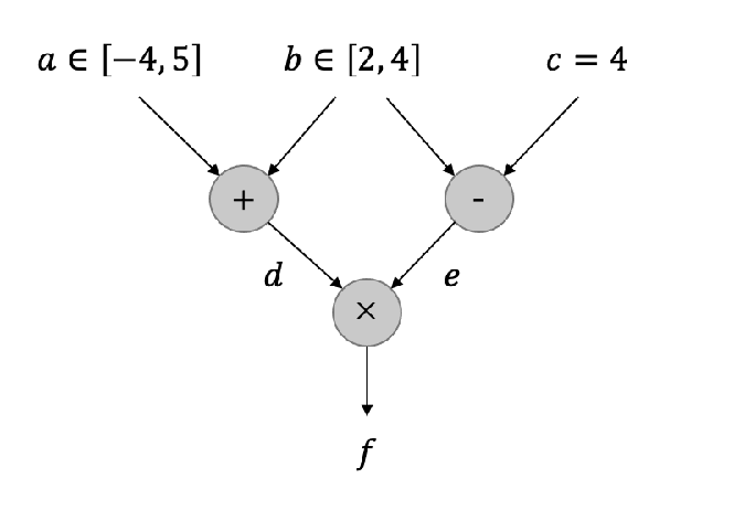
where $\epsilon_{\ast}\in[-1,1]$ is a new uncertainty variable. Note that $uv\epsilon_{\ast}\geq\sum_{i}{(x_{i}\epsilon_{i})}\sum_{i}{(y_{i}\epsilon_{i})}$. See Figure 2 for a simple tutorial of AA.

Division $\hat{z}=\frac{\hat{x}}{\hat{y}}$ is often separated into $\hat{x}\ast\frac{1}{\hat{y}}$. There are mainly two approximation methods to compute $\frac{1}{\hat{y}}$: (1) the min-max approximation and (2) the chebyshev approximation. Here we show the definition of $\frac{1}{\hat{y}}$ with the min-max approximation.

where $a=\mathrm{inf}(\hat{y})$ and $b=\mathrm{sup}(\hat{y})$. Note that $\frac{1}{\hat{y}}$ is defined only if $b>a>0$ or $0>b>a$. The denominator $\hat{y}$ must not include zero.

Suppose we have an affine form $\hat{x}$, the minimum number of integer bits that never cause overflow and underflow is computed by;

$IB$ represents the optimal integer bit-width.

Remember that all input intervals must be known in AA; in other words the intervals of $\{\bm{x}_{1},\ldots,\bm{x}_{N}$, $\bm{t}_{1},\ldots,\bm{t}_{N}$, $\bm{\alpha}$, $\bm{b}$, $\bm{P}_{0}$, $\bm{\beta}_{0}\}$ for training graph and $\{\bm{x},\bm{\alpha},\bm{b},\bm{\beta}\}$ for prediction graph must be given. In this work we assume that the intervals of $\{\bm{x},\bm{x}_{1},\ldots,\bm{x}_{N},\bm{t}_{1},\ldots,\bm{t}_{N}\}$ are $[0,1]$, and those of $\{\bm{\alpha},\bm{b}\}$ are $[-1,1]$. $\{\bm{P}_{0},\bm{\beta}_{0}\}$ is computed by Equation 5. The interval of $\bm{\beta}$ (an input of prediction graph) is computed in the way described in Section 3.3.

The goal of training graph is to find the intervals of $\{\bm{\gamma}_{i}^{(1)},\ldots,\bm{\gamma}_{i}^{(10)}$, $\bm{P}_{i}$, $\bm{\beta}_{i}$, $\bm{e}_{i},\bm{h}_{i}\}$ for $1\leq i\leq N$, however, we have to deal with a critical problem; OS-ELM is an online learning algorithm and the total number of training steps $N$ is unknown as training may occur in runtime (i.e. $N$ can increase in runtime). if $N$ is unknown, the training graph grows endlessly and interval analysis becomes infeasible. We need to determine a “reasonable” value of $N$ for training graph.

Prediction graph takes $\{\bm{x},\bm{\beta}\}$ as input. The interval of $\bm{\beta}$ should be that of $\bm{\beta}_{i}$ over $0\leq i\leq N$, more specifically, $0\leq i\leq 1$ ($N=1$). We propose to compute $\mathrm{min}(\mathrm{inf}(\hat{\beta}_{0[u,v]}),\mathrm{inf}(\hat{\beta}_{1[u,v]}))$ for the lower bound of $\beta_{[u,v]}$ and $\mathrm{max}(\mathrm{sup}(\hat{\beta}_{0[u,v]}),\mathrm{sup}(\hat{\beta}_{1[u,v]}))$ as the upper bound, where $\beta_{[u,v]}$ represents the $uv$ element of $\bm{\beta}$.

In this section we first show the result of the proposed interval analysis method for each dataset, comparing with an ordinary simulation-based interval analysis method. Here is a brief introduction of the simulation method: \scriptsize{1}⃝ Implement OS-ELM’s initialization, prediction, and training algorithms in double-precision format. \scriptsize{2}⃝ Execute initialization algorithm using initial training samples. $\{\bm{P}_{0},\bm{\beta}_{0}\}$ is obtained. \scriptsize{3}⃝ Execute training algorithm by one step using online training samples. $\{\bm{P}_{k},\bm{\beta}_{k}\}$ is obtained if $i=k$. \scriptsize{4}⃝ Generate 1,000 random training samples $\{\bm{x},\bm{t}\}$ with uniform distribution of $[0,1]$. \scriptsize{5}⃝ Feed all the random samples into training algorithm of step = $k$ and measure the values of $\{\bm{\gamma}_{k}^{(1)},\ldots,\bm{\gamma}_{k}^{(10)},\bm{P}_{k},\bm{\beta}_{k},\bm{e}_{k},\bm{h}_{k}\}$. \scriptsize{6}⃝ Feed all the random samples into prediction algorithm and measure the values of $\bm{y}$. \scriptsize{7}⃝ Repeat 3-6 until all online training samples run out.

References

- [1] M. Tsukada, M. Kondo, and H. Matsutani. A Neural Network-based On-device Learning Anomaly Detector for Edge Devices. IEEE Transactions on Computers, 69(7):1027–1044, Jul 2020.
- [2] N.Y. Liang, G.B. Huang, P. Saratchandran, and N. Sundararajan. A Fast and Accurate Online Sequential Learning Algorithm for Feedforward Networks. IEEE Transactions on Neural Networks, 17(6):1411–1423, Nov 2006.
- [3] M. Tsukada, M. Kondo, and H. Matsutani. OS-ELM-FPGA: An FPGA-Based Online Sequential Unsupervised Anomaly Detector. In Proceedings of the International European Conference on Parallel and Distributed Computing Workshops, pages 518–529, Aug 2018.
- [4] J.V.F. Villora, A.R. Muñoz, M.B. Mompean, J.B. Aviles, and J.F.G. Martinez. Moving Learning Machine towards Fast Real-Time Applications: A High-Speed FPGA-Based Implementation of the OS-ELM Training Algorithm. Electronics, 7(11):1–23, Nov 2018.
- [5] A. Safaei, Q.M.J. Wu, T. Akilan, and Y. Yang. System-on-a-Chip (SoC)-based Hardware Acceleration for an Online Sequential Extreme Learning Machine (OS-ELM). IEEE Transactions on Computer-Aided Design of Integrated Circuits and Systems (Early Access), Oct 2018.
- [6] D.U. Lee, A.A. Gaffer, R.C.C Cheung, O. Mencer, W. Luk, and G.A. Constantinides. Accuracy-Guaranteed Bit-Width Optimization. IEEE Transactions on Computer-Aided Design of Integrated Circuits and Systems, 25(10):1990–2000, Oct 2006.
- [7] A. Kinsman and N. Nicolici. Bit-Width Allocation for Hardware Accelerators for Scientific Computing Using SAT-Modulo Theory. IEEE Transactions on Computer-Aided Design of Integrated Circuits and Systems, 29(3):405–413, Mar 2010.
- [8] D. Boland and G. Constantinides. Bounding Variable Values and Round-Off Effects Using Handelman Representations. IEEE Transactions on Computer-Aided Design of Integrated Circuits and Systems, 30(11):1691–1704, Nov 2011.
- [9] J. Stolfi and L. Figueiredo. Self-Validated Numerical Methods and Applications, 1997.
- [10] G.B. Huang, Q.Y. Zhu, and C.K. Siew. Extreme Learning Machine: A New Learning Scheme of Feedforward Neural Networks. In Proceedings of the International Joint Conference on Neural Networks, pages 985–990, Jul 2004.
- [11] D. Menard, G. Caffarena, J. Antonio, A. Lopez, D. Novo, and O. Sentieys. Fixed-point refinement of digital signal processing systems, pages 1–37. The Institution of Engineering and Technology, May 2019.
- [12] R. Cmar, L. Rijnders, P. Schaumont, S. Vernalde, and I. Bolsens. A methodology and design environment for DSP ASIC fixed point refinement. In Design, Automation and Test in Europe Conference and Exhibition, pages 271–276, Mar 1999.
- [13] A. Gaffar, O. Mencer, and W. Luk. Unifying bit-width optimisation for fixed-point and floating-point designs. In The Annual IEEE Symposium on Field-Programmable Custom Computing Machines, pages 79–88, Apr 2004.
- [14] H. Keding, M. Willems, and H. Meyr. Fridge: a fixed-point design and simulation environment. In Design, Automation and Test in Europe Conference and Exhibition, pages 429–435, Feb 1998.
- [15] C. Shi and R. Brodersen. Automated fixed-point data-type optimization tool for signal processing and communication systems. In Design Automation Conference, pages 478–483, July 2004.
- [16] J. Cong, K. Gururaj, B. Liu, C. Liu, Z. Zhang, S. Zhou, and Y. Zou. Evaluation of Static Analysis Techniques for Fixed-Point Precision Optimization. In Proceedings of the IEEE Symposium on Field Programmable Custom Computing Machines, pages 231–234, Apr 2009.
- [17] S. Vakili, J.M.P Langlois, and G. Bois. Enhanced Precision Analysis for Accuracy-Aware Bit-Width Optimization Using Affine Arithmetic. IEEE Transactions on Computer-Aided Design of Integrated Circuits and Systems, 32(12):1853–1865, Dec 2013.
- [18] R. Moore. Interval Analysis. Science, 158(3799):365–365, Oct 1967.
- [19] C.F. Fang, R.A. Rutenbar, and T. Chen. Fast, accurate static analysis for fixed-point finite-precision effects in DSP designs. In Proceedings of the International Conference on Computer Aided Design, pages 1–8, Nov 2003.
- [20] Y. Pu and Y. Ha. An automated, efficient and static bit-width optimization methodology towards maximum bit-width-to-error tradeoff with affine arithmetic model. In Proceedings of the Asia and South Pacific Conference on Design Automation, pages 886–891, Jan 2006.
- [21] S. Wang and X. Qing. A Mixed Interval Arithmetic/Affine Arithmetic Approach for Robust Design Optimization With Interval Uncertainty. Journal of Mechanical Design, 138(4):041403–1–041403–10, Apr 2016.
- [22] R. Bellal, E. Lamini, H. Belbachir, S. Tagzout, and A. Belouchrani. Improved Affine Arithmetic-Based Precision Analysis for Polynomial Function Evaluation. IEEE Transactions on Computers, 68(5):702–712, May 2019.
- [23] E. Alpaydin and C. Kaynak. Optical Recognition of Handwritten Digits Data Set. https://archive.ics.uci.edu/ml/datasets/Optical+Recognition+of+Handwritten+Digits, 1998.
- [24] Digilent PYNQ-Z1. https://japan.xilinx.com/products/boards-and-kits/1-hydd4z.html.
- [25] R. Fisher. Iris Data Set. http://archive.ics.uci.edu/ml/datasets/Iris/, 1936.
- [26] D. Slate. Letter Recognition Data Set. https://archive.ics.uci.edu/ml/datasets/Letter+Recognition, 1890.
- [27] I. Yeh. Default of Credit Card. https://archive.ics.uci.edu/ml/datasets/default+of+credit+card+clients, 2016.
- [28] M. Bator. Sensorless Drive Diagnosis. https://archive.ics.uci.edu/ml/datasets/dataset+for+sensorless+drive+diagnosis, 2015.