Modeling and simulation of nuclear architecture reorganization process using a phase field approachThanks: The work is partially supported by NSF Grant DMS-1720442 and AFOSR Grant FA9550-16-1-0102.

Qing Cheng Thanks: Department of Mathematics,Purdue University, West Lafayette, IN 47907, USA (cheng573$@$purdue.edu, shen7$@$purdue.edu). Pourya Delafrouz Thanks: Department of Bioengineering, University of Illinois at Chicago, SEO, MC-063, Chicago, IL, 60607-7052, USA (pdelaf2$@$uic.edu, jliang$@$uic.edu). Jie Liang^‡ Chun Liu Thanks: Department of Applied Mathematics, Illinois Institute of Technology, Chicago, IL 60616, USA (cliu124$@$iit.edu). Jie Shen^†

Abstract

We develop a special phase field/diffusive interface method to model the nuclear architecture reorganization process. In particular, we use a Lagrange multiplier approach in the phase field model to preserve the specific physical and geometrical constraints for the biological events. We develop several efficient and robust linear and weakly nonlinear schemes for this new model. To validate the model and numerical methods, we present ample numerical simulations which in particular reproduce several processes of nuclear architecture reorganization from the experiment literature.

1 Introduction

Genetic information is transmitted through genome and exhibits a hierarchical structure in the nucleus. The cell nucleus and the genome are organized into spatially separated sub-compartments [12]. For eukaryotes, genetic information is stored in DNA which is also integrated into chromosomes of a cell nucleus [12, 22, 29, 8]. In chromosome territory, chromatin fibers are formed when DNA molecule is wrapped around the histones, and form transcriptionally inactivated and condensed region form as heterochromatin and transcriptionally activated region form euchromatin. The position, structure and configuration of heterochromatin and euchromatin regions are closely related to the gene expression. For instance, it has been observed that the volume of cell nucleus is a main determinant of the overall landscape of chromatin folding [16, 18, 17]. Different kinds of nuclear architecture can attribute to different distribution and configuration of heterochromatin and euchromatin regions [30, 6], with additional protein-mediated specific interactions among genomic elements [25, 31]. Moreover, the inverted architecture occurs where heterochromatin is located at the center of the nucleus and euchromatin is enriched at the periphery. In contrast, when the heterochromatin is enriched at the nuclear periphery and around nucleoli, this is referred as the conventional architecture.

In [28, 29], Solovei et al. demonstrated that different types of nuclear architecture were associated with different mammalian lifestyles, such as diurnal versus nocturnal. The inverted nuclear architecture can be transformed from the convention architecture in mouse retina rod cells [28, 29]. The reorganization process is accompanied by the relocation of chromosomes from positions enriched at nuclear periphery, and the recreation of a single heterochromatin cluster into the inverted architecture. The difference of nuclear structure is partially attributed to the activity of lamin B, lamin A and envelope proteins [24, 28, 29, 20, 33]. Moreover, the rate of conversion of heterochromatin to euchromatin can also be controlled by volume constraints of the nucleus.

Recently several mathematical models using the phase field approach [21, 22, 27] have been introduced to study the mechanism of generation of different nuclear architectures, including the size and shape of the nucleus, the rate of conversion of heterochromatin to euchromatin. These models usually include the minimization of total energy with various relevant geometric constraints. A common method to preserve such constraints is through extra penalty terms introduced in the energy functionals in models [21, 22]. The drawback of such methods is the presence of the large penalty parameters which results in a stiff nuclear architecture reorganization systems, leading to significant challenge in the simulation and analysis. This is especially true in situations when the volume of chromosome must be enforced during the reduction of nuclear size and reorganization of nuclear architectures.

The Lagrange multiplier approach is commonly used for constrained gradient dynamic systems [11, 10, 9, 19, 36, 35, 34, 4]. In this paper, we introduce a new Lagrange multiplier approach [3, 5, 32] to enforce the geometric constraints such as the volume constraints for both chromosome and heterochromatin. When the volumes of each chromosome and heterochromatin are preserved as constants, the reaction-diffusion system with the Lagrange multipliers leads to a constrained gradient flow dynamics which satisfies an energy dissipation law. We develop several numerical schemes for nuclear architecture system with Lagrange multipliers. One is a weakly nonlinear scheme which preserves the volume constraints but requires solving a set of $2\times 2$ nonlinear algebraic systems for the Lagrange multipliers, the second is a purely linear scheme which approximates the volume constraints to second order and only requires solving linear systems with constant coefficient. These two schemes, while being numerically efficient, do not satisfy a discrete energy law. Hence, we construct the third scheme which is also weakly nonlinear but is unconditionally energy stable. However, this scheme requires solving a nonlinear algebraic system of $2N+1$ (where $N$ is the number of chromosomes in the nucleus) equations which may require smaller time steps to be well posed. One can choose to use one of these schemes in different scenarios. In our numerical simulations, we use the first scheme to control the volumes to targeted values exactly, then we switch to the second scheme which is more efficient. We can use the third scheme if we want to make sure that the scheme is energy dissipative.

For validation purpose, we present several simulations results which are consistent with those observed in the experiments. We also demonstrate that our model and schemes are efficient and robust for investigating various nuclear architecture reorganization processes.

The paper is organized as follows: in Section 2, we present our phase field model for nuclear architecture reorganization by using a Lagrange multiplier approach. We chose suitable energy functionals to capture the most important interactions and constraints of various biological elements, and introduce Lagrange multipliers to capture the specific geometric constraints for the biological process. In Section 3, we develop efficient linear and weakly nonlinear time discretization schemes for the phase field model developed earlier. We present numerical results using the proposed schemes in Section 4, and compare them with the existing experimental literature and previous works. Finally we conclude the paper with more discussions of our methods and results in Section 5.

2 A phase field model for nuclear architecture reorganization (NAR)

To study the nuclear architecture reorganization (NAR) process, we employ a phase field/diffusive interface method. To start with this approach, the total nucleus is defined by a phase (labeling) function $\phi_{0}$ such that $\phi_{0}=0$ and $\phi_{0}=1$ respectively for the interior and exterior regions of the nucleus (Fig. 2). For a ellipsoid shape domain, we can define

\phi_{0}(x,y,t)=\frac{1}{2}(1-\tanh(\frac{\sqrt{\frac{x^{2}}{r^{2}_{x}(t)}+\frac{y^{2}}{r^{2}_{y}(t)}}-1}{\sqrt{2}\epsilon})),

(2.1)

where $\epsilon$ is the interfacial (transitional domain) width, ${r}_{x}(t)$ and ${r}_{y}(t)$ describe the ellipse shape of the nucleus. Similarly, we will introduce phase functions $\psi$ to describe the heterochromatin region and $\boldsymbol{\phi}=(\phi_{1},\phi_{2},\cdots,\phi_{N})$ to describe each individual chromosome region, where $N$ represents the total number of chromosomes in the nucleus ( Fig. 2). In particular, we will choose $N=8$ chromosomes for drosophila and $N=46$ chromosomes for human. In addition to the heterochromatin region, the rest of chromosome region is the euchromatin region. These are the order parameter/phase field functions that will be used to determined the final nuclear architecture.

For the general phase field approaches, the configuration and distribution of various regions are the consequence of minimizing a specific energy functional in terms of the above phase field functions, which takes into all considerations of the coupling and competition between different domains, as well as the relevant geometry constraints.

In the NAR models [22, 21], the free energy for chromosome and heterochromatin had been chosen to include

E_{0}(\boldsymbol{\phi},\psi)=\sum\limits_{m=1}^{N}\int_{\Omega}\frac{\epsilon_{\phi}^{2}}{2}|\nabla\phi_{m}|^{2}+g(\phi_{m})d\boldsymbol{x}+\int_{\Omega}\frac{\epsilon_{\psi}^{2}}{2}|\nabla\psi|^{2}+g(\psi)d\boldsymbol{x},

(2.2)

where $\epsilon_{\phi}$ and $\epsilon_{\psi}$ measure the interfacial thickness corresponding to $\phi$ and $\psi$ , $\Omega$ is the computational domain, and $g(\phi)=\frac{1}{4}\phi^{2}(1-\phi)^{2}$ is the double well potential which possess the local minima at $\phi=0$ and $\phi=1$ (see [26]). This part of free energy represents the competition and coupling between various chromosome and heterochromatin regions.

Next we will consider the following geometric constraints for all these regions that are biologically relevant to our application [1, 7]:

1.

All chromosomes are restricted within the cell nucleus region;
2.

Heterochromosome of each chromosome stays within the chromosome;
3.

Between all chromosomes, due to the excluded volume effects, do not self-cross or cross each other.

These constraints could be incorporated into the model by introducing three extra terms in the free energy:

\begin{split}E_{1}(\boldsymbol{\phi},\psi)&=\underbrace{\beta_{0}\sum\limits_{m=1}^{N}\int_{\Omega}h(\phi_{0})h(\phi_{m})d\boldsymbol{x}}_{1}+\underbrace{\beta_{\psi}\int_{\Omega}[1-\sum\limits_{m=1}^{N}h(\phi_{m})]h(\psi)d\boldsymbol{x}}_{2}\\ &+\underbrace{\beta_{\phi}\sum\limits_{m\neq n}\int_{\Omega}h(\phi_{n})h(\phi_{m})d\boldsymbol{x}}_{3},\end{split}

(2.3)

where $\beta_{0},\beta_{\psi}$ and $\beta_{\phi}$ are three positive constants which indicate the intensities of domain territories, and $h(\phi)$ is used for the induction of driving interface between $\phi=0$ and $\phi=1$ while keeping the local minima $0$ and $1$ fixed during dynamic process. The required conditions for $h(\phi)$ are

h(0)=0,\;h(1)=1,\;h^{\prime}(0)=h^{\prime}(1)=h^{\prime\prime}(0)=h^{\prime\prime}(1)=0.

(2.4)

The lowest degree polynomials satisfying the above conditions is $h(\phi)=\phi^{3}(10-15\phi+6\phi^{2})$ , see Fig. 1.

Refer to caption — Figure 1: The function $h(\phi)=\phi^{3}(10-15\phi+6\phi^{2})$ .

Due to the expression of LBR and lamin A/C in the nuclear envelope, interactions between heterochromatin and the nuclear envelope play an important role in nuclear architecture reorganization process. For this purpose, another term was introduced in the free energy to describe the interactions [29]:

E_{2}(\phi_{0},\psi)=\gamma\int_{\Omega}\nabla h(\phi_{0})\cdot\nabla h(\psi)d\boldsymbol{x},

(2.5)

where $\gamma$ is the affinity constant, and $\gamma>0$ implies the heterochromatin will locate at the nuclear periphery, while $\gamma=0$ leads to the lack of heterochromatin and nuclear envelope interactions due to the absence of LBR or lamin A/C. More precisely, $E_{2}$ represents the intensity of affinity between nuclear function $\phi_{0}$ and heterochromatin region function $\psi$ .

2.1 NAR model with Lagrange multipliers

In the general nuclear reorganization process, often one need to take into account more geometric constraints. In particular, we shall include the following constraints in our model:

4.

The nuclear space is fully occupied by chromosomes;
5.

Heterochromatin is converted from/to euchromatin within each chromosome.

Notice that our approach could be extended to more general situations, especially related to those of item 4.

Our approach here is to introduce Lagrange multipliers to guarantee the constraints $4,5$ in the following NAR model with the total free energy

E(\phi_{0},\boldsymbol{\phi},\psi)=E_{0}+E_{1}+E_{2}.

(2.6)

The corresponding Allen-Cahn type gradient flow [23, 3, 13, 2, 15, 14, 36] with respect to the above energy and the constraints 4 and 5 take the form:

	$\displaystyle\frac{\partial\phi_{m}}{\partial t}=-M\Big\{\frac{\delta E}{\delta\phi_{m}}-\lambda_{m}h^{\prime}(\phi_{m})-\eta_{m}h^{\prime}(\phi_{m})h(\psi)\Big\},\quad m=1,2,\cdots,N,$		(2.7)
	$\displaystyle\frac{\partial\psi}{\partial t}=-M\Big\{\frac{\delta E}{\delta\psi}-\sum\limits_{m=1}^{N}\eta_{m}h(\phi_{m})h^{\prime}(\psi)\Big\},$		(2.8)
	$\displaystyle V_{m}(t)=\int_{\Omega}h(\phi_{m})d\boldsymbol{x},\qquad v_{m}(t)=\int_{\Omega}h(\phi_{m})h(\psi)d\boldsymbol{x},\quad m=1,2,\cdots,N,$		(2.9)
	$\displaystyle\sum\limits_{m=1}^{N}V_{m}(t)=\int_{\Omega}h(\phi_{0})d\boldsymbol{x},$		(2.10)

where $M$ is mobility constant, $V_{m}(t)$ and $v_{m}(t)$ $(m=1,2,\cdots,N)$ represent, respectively. From (2.9), the volume of chromosome can be contracted or expanded to a given volume by using our model. The volumes of $m$ -th chromosome and heterochromatin in the $m$ -th chromosome at time $t$ during nuclear reorganization (growth or inversion) stage are enforced by the Lagrange multipliers $\lambda_{m}(t)$ , $\eta_{m}(t)$ $(m=1,2,\cdots,N)$ (2.9). The boundary conditions can be one of the following two types

\displaystyle(i)\mbox{ periodic; or }(ii)\,\,\partial_{\bf n}\phi_{m}|_{\partial\Omega}=\partial_{\bf n}\psi|_{\partial\Omega}=0,

(2.11)

where $\bf n$ is the unit outward normal on the boundary $\partial\Omega$ .

Let $\bar{V}_{m}$ and $\bar{v}_{m}$ be, respectively, the target volumes for each chromosome and heterochromatin in each chromosome, $\rho_{m}(t)=v_{m}(t)/V_{m}(t)$ can be interpreted as the heterochromatin conversion rate during nuclear architecture reorganization process. We assume that they will reach the target values at time $t=t_{0}$ and then stay there according to:

\begin{split}&V_{m}(t)=\begin{cases}V_{m}(0)+\frac{(\bar{V}_{m}+\delta_{1m})t}{t+\alpha_{1}e^{-\alpha_{2}t}},&0\leq t\leq t_{0}\\ \bar{V}_{m},&t\geq t_{0}\end{cases};\\ &v_{m}(t)=\begin{cases}v_{m}(0)+\frac{(\bar{v}_{m}+\delta_{2m})t}{t+\alpha_{1}e^{-\alpha_{2}t}},&0\leq t\leq t_{0}\\ \bar{v}_{m},&t\geq t_{0}\end{cases},\end{split}

(2.12)

where $\delta_{1m}$ and $\delta_{2m}$ are determined by $V_{m}(t_{0})=\bar{V}_{m}$ and $v_{m}(t_{0})=\bar{v}_{m}$ . and $\alpha_{i}$ $(i=1,2)$ are suitable positive constants related to the time scale. Similarly, we assume that $r_{x}(t)$ and $r_{y}(t)$ evolve according to

\begin{split}&r_{x}(t)=\begin{cases}r_{x}(0)+\frac{(\bar{r}_{x}+\delta_{3})t}{t+\alpha_{1}e^{-\alpha_{2}t}},&0\leq t\leq t_{0}\\ \bar{V}_{m},&t\geq t_{0}\end{cases};\\ &r_{y}(t)=\begin{cases}r_{y}(0)+\frac{(\bar{r}_{y}+\delta_{4})t}{t+\alpha_{1}e^{-\alpha_{2}t}},&0\leq t\leq t_{0}\\ \bar{v}_{m},&t\geq t_{0}\end{cases},\end{split}

(2.13)

where $\delta_{3}$ and $\delta_{4}$ are determined by $r_{x}(t_{0})=\bar{r}_{x}$ and $r_{y}(t_{0})=\bar{r}_{y}$ with $\bar{r}_{x}$ and $\bar{r}_{y}$ being the targeted axis lengths for the ellipse enclosing the nucleus.

Remark 2.1.

In [22], a penalty approach is introduced to satisfy the physical constraints 4 and 5 by adding the following to the free energy:

\begin{split}E_{2}(\boldsymbol{\phi},\psi)&=\underbrace{\alpha_{0}[\int_{\Omega}[1-h(\phi_{0})]dx-\sum\limits_{m=1}^{N}V_{m}(t)]^{2}}_{4}+\underbrace{\alpha_{V}\sum\limits_{m=1}^{N}[V_{m}(t)-\bar{V}_{m}(t)]^{2}}_{5}\\ &+\underbrace{\alpha_{v}\sum\limits_{m=1}^{N}[v_{m}(t)-\bar{v}_{m}(t)]^{2}}_{6},\end{split}

(2.14)

where $\alpha_{0},\alpha_{V},\alpha_{v}$ are three positive penalty parameters. The volume of $m$ -th chromosome $V_{m}(t)$ and volume of heterochromatin in $m$ -th chromosome are defined in (2.9). A disadvantage of the penalty approach is large penalty parameters are needed for accurate approximation of the physical constraints, and may lead to very stiff systems that are difficult to solve numerically. The Lagrange multiplier approach that we use here can enforce these non-local constraints exactly and is free of penalty parameters. Furthermore, the NAR model (2.7)-(2.10) based on the Lagrange multiplier approach can control exactly the growth rate of volume for different compartments during the nuclear reorganization (growth or inversion).

Remark 2.2.

In the phase field approaches, there are many ways to represent the volume of each individual domain. For instance, the volume of each chromosome denoted by $V_{m}(t)$ and their corresponding heterochromatin domain volume $v_{m}(t)$ could be computed by the integrals $\int_{\Omega}\phi_{m}d\boldsymbol{x}$ and $\int_{\Omega}\psi d\boldsymbol{x}$ . However this representation may have disadvantages in the minimizing procedure, especially for the penalty methods used in [21, 22, 27], due to its linearity with respect to the phase functions. One way to overcome this is to use the polynomial function $h(\phi)=\phi^{3}(10-15\phi+6\phi^{2})$ (see Fig. 1) for the computation of the volumes for different chromosome regions. Since $h(\phi)$ is an increasing function with respect to $\phi$ in the interval $[0,1]$ with $h(0)=0$ and $h(1)=1$ . One can adapt $V_{m}=\int_{\Omega}h(\phi)d\boldsymbol{x}$ and $\int_{\Omega}h(\phi_{m})h(\psi)d\boldsymbol{x}$ for the volume of $m$ -th chromosome and heterochromatin in $m$ -th chromosome.

Let $(\cdot,\cdot)$ be the inner product in $L^{2}(\Omega)$ , and $\|\cdot\|$ be the associated norm in $L^{2}(\Omega)$ . The constrained NAR model (2.7)-(2.10) with (2.12) can be interpreted as a $L^{2}$ gradient system which implies phase separations will happen for $t\geq t_{0}$ .

Theorem 1.

The constrained NAR model (2.7)-(2.10) with (2.12) satisfies the following energy dissipation law

\frac{d}{dt}E(\phi_{0},\boldsymbol{\phi},\psi)=-\frac{1}{M}(\sum\limits_{m=1}^{N}\|\partial_{t}\phi_{m}\|^{2}+\|\partial_{t}\psi\|^{2}),\quad\forall t\geq t_{0}.

(2.15)

Proof.

Taking the inner product of (2.7) with $\partial_{t}\phi_{m}$ , we obtain

\begin{split}-\frac{1}{M}\|\frac{\partial\phi_{m}}{\partial t}\|^{2}&=(\frac{\delta E}{\delta\phi_{m}},\partial_{t}\phi_{m})-\lambda_{m}(h^{\prime}(\phi_{m}),\partial_{t}\phi_{m})\\ &-\eta_{m}(h^{\prime}(\phi_{m})h(\psi),\partial_{t}\phi_{m}).\end{split}

(2.16)

Taking the inner product of (2.8) with $\partial_{t}\psi$ , we obtain

\begin{split}-\frac{1}{M}\|\frac{\partial\psi}{\partial t}\|^{2}=(\frac{\delta E}{\delta\psi},\partial_{t}\psi)-\sum\limits_{m=1}^{N}\eta_{m}(h(\phi_{m})h^{\prime}(\psi),\partial_{t}\psi).\end{split}

(2.17)

We derive from (2.9) that

(h^{\prime}(\phi_{m}),\partial_{t}\phi_{m})=\frac{d}{dt}\int_{\Omega}h(\phi_{m})d\boldsymbol{x}=\frac{d}{dt}\bar{V}_{m}=0.

(2.18)

Similarly, we obtain

(h^{\prime}(\phi_{m})h(\psi),\partial_{t}\phi_{m})+(h(\phi_{m})h^{\prime}(\psi),\partial_{t}\psi)=\frac{d}{dt}\int_{\Omega}h(\phi_{m})h(\psi)d\boldsymbol{x}=\frac{d}{dt}\bar{v}_{m}=0.

(2.19)

Summing up (2.16) for $m=1,2,\cdots,N$ , combing it with (2.17)-(2.19) and using equality

\sum\limits_{m=1}^{N}(\frac{\delta E}{\delta\phi_{m}},\partial_{t}\phi_{m})+(\frac{\delta E}{\delta\psi},\partial_{t}\psi)=\frac{d}{dt}E(\phi_{0},\boldsymbol{\phi},\psi),

(2.20)

we obtain the desired energy dissipation law (2.15).

3 Numerical Schemes

In this section, we construct several efficient time discretization schemes based on the Lagrange multiplier approach [3, 5] for the phase field NAR model (2.7)-(2.10). For the sake of simplicity, for any function $f$ , we denote $f^{n,\dagger}=2f^{n}-f^{n-1}$ , $f^{n,\star}=\frac{3}{2}f^{n}-\frac{1}{2}f^{n-1}$ and $f^{n+\frac{1}{2}}=\frac{f^{n+1}+f^{n}}{2}$ .

We split the total energy into a quadratic part and the remaining part as follows:

E(\phi_{0},\boldsymbol{\phi},\psi)=\big(\sum\limits_{m=1}^{N}\int_{\Omega}\frac{\epsilon_{\phi}^{2}}{2}|\nabla\phi_{m}|^{2}d\boldsymbol{x}+\int_{\Omega}\frac{\epsilon_{\psi}^{2}}{2}|\nabla\psi|^{2}d\boldsymbol{x}\big)+\tilde{E}(\phi_{0},\boldsymbol{\phi},\psi),

where $\tilde{E}$ is

\begin{split}\tilde{E}(\phi_{0},\boldsymbol{\phi},\psi)=&\beta_{0}\sum\limits_{m=1}^{N}\int_{\Omega}h(\phi_{0})h(\phi_{m})d\boldsymbol{x}+\beta_{\psi}\int_{\Omega}[1-\sum\limits_{m=1}^{N}h(\phi_{m})]h(\psi)d\boldsymbol{x}\\ &+\beta_{\phi}\sum\limits_{m\neq n}\int_{\Omega}h(\phi_{n})h(\phi_{m})d\boldsymbol{x}+\sum\limits_{m=1}^{N}\int_{\Omega}g(\phi_{m})d\boldsymbol{x}+\int_{\Omega}g(\psi)d\boldsymbol{x}\\ &+\gamma\int_{\Omega}\nabla h(\phi_{0})\cdot\nabla h(\psi)d\boldsymbol{x}.\end{split}

(3.21)

Once the volume of nucleus $\int_{\Omega}h(\phi_{0})d\boldsymbol{x}$ is given, volumes of each chromosome territory can be set up accordingly so that the constraint (2.10) can be satisfied automatically.

3.1 A weakly nonlinear volume preserving scheme

Note that in the first stage, we need to increase the volumes $V_{m}(t)$ and $v_{m}(t)$ to the targeted values $\bar{V}_{m}$ and $\bar{v}_{m}$ according to (2.12), respectively. Hence, we shall first construct below a volume preserving scheme which allows us to achieve this goal. More precisely, a second order scheme based on the Lagrange multiplier approach is as follows:

$\displaystyle\frac{\phi^{n+1}_{m}-\phi_{m}^{n}}{\delta t}$	$\displaystyle=-M(-\epsilon^{2}_{\phi}\Delta\phi^{n+\frac{1}{2}}_{m}$
	$\displaystyle+(\frac{\delta\tilde{E}}{\delta\phi_{m}})^{n,\star}-\lambda^{n+\frac{1}{2}}_{m}h^{\prime}(\phi^{n,\star}_{m})-\eta^{n+\frac{1}{2}}_{m}h^{\prime}(\phi^{n,\star}_{m})h(\psi^{n,\star})),\;m=1,\cdots,N,$	(3.22)
$\displaystyle\frac{\psi^{n+1}-\psi^{n}}{\delta t}$	$\displaystyle=-M(-\epsilon^{2}_{\psi}\Delta\psi^{n+\frac{1}{2}}+(\frac{\delta\tilde{E}}{\delta\psi})^{n,\star}-\sum\limits_{m=1}^{N}\eta_{m}^{n+\frac{1}{2}}h(\phi^{n,\star}_{m})h^{\prime}(\psi^{n,\star})),$	(3.23)
$\displaystyle V_{m}(t^{n+1})$	$\displaystyle=\int_{\Omega}h(\phi^{n+1}_{m})d\boldsymbol{x},\;m=1,\cdots,N,$	(3.24)
$\displaystyle v_{m}(t^{n+1})$	$\displaystyle=\int_{\Omega}h(\phi^{n+1}_{m})h(\psi^{n+1})d\boldsymbol{x},\;m=1,\cdots,N.$	(3.25)

Below we show how to efficiently solve the coupled scheme (3.22)-(3.25). Writing

\begin{split}&\phi_{m}^{n+1}=\phi_{1,m}^{n+1}+\lambda_{m}^{n+\frac{1}{2}}\phi_{2,m}^{n+1}+\eta_{m}^{n+\frac{1}{2}}\phi_{3,m}^{n+1},\end{split}

(3.26)

in (3.22), collecting all terms without $(\lambda_{m}^{n+1},\eta_{m}^{n+1})$ , with $\lambda_{m}^{n+1}$ or with $\eta_{m}^{n+1}$ , we find that, for $m=1,2,\cdots,N$ , $(\phi_{i,m}^{n+1},\,i=1,2,3)$ can be determined from the following decoupled linear systems:

\begin{split}&\frac{\phi^{n+1}_{1,m}-\phi_{m}^{n}}{\delta t}=-M(-\epsilon^{2}_{\phi}\Delta\phi^{n+\frac{1}{2}}_{1,m}+(\frac{\delta\tilde{E}}{\delta\phi_{m}})^{n,\star});\end{split}

(3.27)

\begin{split}&\frac{\phi^{n+1}_{2,m}}{\delta t}=-M(-\epsilon^{2}_{\phi}\Delta\phi^{n+\frac{1}{2}}_{2,m}-h^{\prime}(\phi^{n,\star}_{m}));\end{split}

(3.28)

\begin{split}&\frac{\phi^{n+1}_{3,m}}{\delta t}=-M(-\epsilon^{2}_{\phi}\Delta\phi^{n+\frac{1}{2}}_{3,m}-h^{\prime}(\phi^{n,\star}_{m})h(\psi^{n,\star})).\end{split}

(3.29)

Then, writing

\begin{split}&\psi^{n+1}=\psi_{1}^{n+1}+\sum\limits_{m=1}^{N}\eta_{m}^{n+\frac{1}{2}}\psi_{2,m}^{n+1},\end{split}

(3.30)

in (3.23), we find that $\psi_{1}^{n+1}$ and $(\psi_{2,m}^{n+1},\,m=1,2,\cdots,N)$ can be determined from the following decoupled linear systems:

\begin{split}&\frac{\psi^{n+1}_{1}-\psi^{n}}{\delta t}=-M(-\epsilon^{2}_{\psi}\Delta\psi_{1}^{n+\frac{1}{2}}+(\frac{\delta\tilde{E}}{\delta\psi})^{n,\star});\end{split}

(3.31)

\begin{split}&\frac{\psi^{n+1}_{2,m}}{\delta t}=-M(-\epsilon^{2}_{\psi}\Delta\psi_{2,m}^{n+\frac{1}{2}}+h(\phi^{n,\star}_{m})h^{\prime}(\psi^{n,\star})).\end{split}

(3.32)

We observe that the above systems are all linear Poisson-type equation with constant coefficients so they can be efficiently solved.

Once we have obtained $(\phi_{i,m}^{n+1},\,i=1,2,3)$ and $\psi_{i,m}^{n+1},\,i=1,2)$ , we plug (3.26)-(3.30) into (3.24)-(3.25) to obtain a $2\times 2$ nonlinear algebraic system for $(\lambda_{m}^{n+1},\eta_{m}^{n+1})$ . For $\delta t$ sufficiently small, this nonlinear algebraic system admits real solutions that be solved with an iterative method at negligible cost.

In summary, the scheme (3.22)-(3.25) can be efficiently implemented as follows.

•

Solve $\psi_{1}^{n+1}$ from (3.31).
•
For $m=1,\cdots,N$ :
- –
  
  solve $(\phi_{i,m}^{n+1},\,i=1,2,3)$ from (3.27)-(3.29) and $\psi_{2,m}^{n+1}$ from (3.32);
- –
  
  determine the Lagrange multipliers $(\lambda_{m}^{n+1},\eta_{m}^{n+1})$ from the coupled nonlinear algebraic system (3.24)-(3.25);
- –
  
  update $\phi_{m}^{n+1}$ using (3.26).
•

Update $\psi^{n+1}$ using (3.30).

3.2 A linear scheme

In practice, the scheme (3.22)-(3.25) should be used if we want to exactly preserve the volume dynamics of chromosome and heterochromatin. A disadvantage of the scheme (3.22)-(3.25) is that we need to solve a nonlinear algebraic system which may require small time steps. To accelerate the simulation, we construct below a linear scheme for system (2.7)-(2.10) which is more efficient but only approximately preserve the volume dynamics.

To this end, we reformulate (2.7)-(2.10) into the following equivalent system:

	$\displaystyle\hskip 56.9055pt\frac{\partial\phi_{m}}{\partial t}=-M\big(-\epsilon^{2}_{\phi}\Delta\phi_{m}+\frac{\delta\tilde{E}}{\delta\phi_{m}}-\lambda_{m}h^{\prime}(\phi_{m})-\eta_{m}h^{\prime}(\phi_{m})h(\psi)\big),\quad m=1,\cdots,N,$		(3.33)
	$\displaystyle\hskip 56.9055pt\frac{\partial\psi}{\partial t}=-M\big(-\epsilon^{2}_{\psi}\Delta\psi+\frac{\delta\tilde{E}}{\delta\psi}-\sum\limits_{m=1}^{N}\eta_{m}h(\phi_{m})h^{\prime}(\psi)\big),$		(3.34)
	$\displaystyle\hskip 56.9055ptV^{\prime}_{m}(t)=\int_{\Omega}h^{\prime}(\phi_{m})\partial_{t}\phi_{m}d\boldsymbol{x},\quad m=1,\cdots,N,$		(3.35)
	$\displaystyle\hskip 56.9055ptv^{\prime}_{m}(t)=\int_{\Omega}h^{\prime}(\phi_{m})h(\psi)\partial_{t}\phi_{m}+h(\phi_{m})h^{\prime}(\psi)\partial_{t}\psi d\boldsymbol{x},\quad m=1,\cdots,N.$		(3.36)

Note that the last two relations are obtained by taking the time derivative of $V_{m}$ and $v_{m}$ in (2.9).

A second-order linear scheme for the new system (3.33)-(3.36) is as follows:

$\displaystyle\frac{\phi^{n+1}_{m}-\phi_{m}^{n}}{\delta t}$	$\displaystyle=-M\big(-\epsilon^{2}_{\phi}\Delta\phi^{n+\frac{1}{2}}_{m}+(\frac{\delta\tilde{E}}{\delta\phi_{m}})^{n,\star}$
	$\displaystyle-\lambda^{n+\frac{1}{2}}_{m}h^{\prime}(\phi^{n,\star}_{m})-\eta^{n+\frac{1}{2}}_{m}h^{\prime}(\phi^{n,\star}_{m})h(\psi^{n,\star})\big),\;m=1,\cdots,N,$	(3.37)
$\displaystyle\frac{\psi^{n+1}-\psi^{n}}{\delta t}$	$\displaystyle=-M\big(-\epsilon^{2}_{\psi}\Delta\psi^{n+\frac{1}{2}}+(\frac{\delta\tilde{E}}{\delta\psi})^{n,\star}-\sum\limits_{m=1}^{N}\eta_{m}^{n+\frac{1}{2}}h(\phi^{n,\star}_{m})h^{\prime}(\psi^{n,\star})\big),$	(3.38)
$\displaystyle V_{m}(t^{n+1})-V_{m}(t^{n})$	$\displaystyle=\int_{\Omega}h^{\prime}(\phi^{n,\star}_{m})(\phi_{m}^{n+1}-\phi_{m}^{n})d\boldsymbol{x},\;m=1,\cdots,N,$	(3.39)
$\displaystyle v_{m}(t^{n+1})-v_{m}(t^{n})$	$\displaystyle=\int_{\Omega}h^{\prime}(\phi^{n,\star}_{m})h(\psi^{n,\star})(\phi_{m}^{n+1}-\phi_{m}^{n})$
	$\displaystyle+h(\phi^{n,\star}_{m})h^{\prime}(\psi^{n,\star})(\psi^{n+1}-\psi^{n})d\boldsymbol{x},\;m=1,\cdots,N.$	(3.40)

The above coupled scheme can be solved in essentially the same fashion as the scheme (3.22)-(3.25). In fact, setting

\begin{split}&\phi_{m}^{n+1}=\phi_{1,m}^{n+1}+\lambda_{m}^{n+\frac{1}{2}}\phi_{2,m}^{n+1}+\eta_{m}^{n+\frac{1}{2}}\phi_{3,m}^{n+1},\end{split}

(3.41)

in (3.37), we find that for $m=1,2,\cdots,N$ , $(\phi_{i,m}^{n+1},\,i=1,2,3)$ are still determined from (3.27)- (3.29). Then, writing

\begin{split}&\psi^{n+1}=\psi_{1}^{n+1}+\sum\limits_{m=1}^{N}\eta_{m}^{n+\frac{1}{2}}\psi_{2,m}^{n+1},\end{split}

(3.42)

in (3.38), we find that $\psi_{1}^{n+1}$ and $(\psi_{2,m}^{n+1},\,m=1,2,\cdots,N)$ are also determined from (3.31)- (3.32). Once we have obtained $(\phi_{i,m}^{n+1},\,i=1,2,3)$ and $\psi_{i,m}^{n+1},\,i=1,2)$ , we plug (3.41)-(3.42) into (3.39)-(3.40) to obtain a $2\times 2$ linear algebraic system for $(\lambda_{m}^{n+1},\eta_{m}^{n+1})$ that can be solved explicitly. In summary, the scheme (3.37)-(3.40) can be efficiently implemented as follows.

•

Solve $\psi_{1}^{n+1}$ from (3.31).
•
For $m=1,\cdots,N$ :
- –
  
  solve $(\phi_{i,m}^{n+1},\,i=1,2,3)$ from (3.27)-(3.29) and $\psi_{2,m}^{n+1}$ from (3.32);
- –
  
  determine the Lagrange multipliers $(\lambda_{m}^{n+1},\eta_{m}^{n+1})$ from the coupled linear algebraic system (3.39) and (3.40);
- –
  
  update $\phi_{m}^{n+1}$ using (3.26).
•

Update $\psi^{n+1}$ using (3.30).

Note that the scheme (3.37)-(3.40) is well posed for any time step.

3.3 A weakly nonlinear energy stable scheme

Note that the schemes (3.22)-(3.25) and (3.37)-(3.40) are not guaranteed to be energy dissipative. Below we modify the scheme (3.22)-(3.25) slightly to construct a weakly nonlinear but energy stable scheme with essentially the same computational cost for $t\geq t_{0}$ when volumes of each chromosome $V_{m}(t)$ and heterochromatin $v_{m}(t)$ become constants.

The idea is to introduce another Lagrange multiplier to enforce the energy dissipation. To this end, we introduce another Lagrange multiplier $R(t)$ and expand the system (3.33)-(3.36) for $t\geq t_{0}$ as

	$\displaystyle\frac{\partial\phi_{m}}{\partial t}=-M\big(-\epsilon^{2}_{\phi}\Delta\phi_{m}+R(t)\frac{\delta\tilde{E}}{\delta\phi_{m}}-\lambda_{m}h^{\prime}(\phi_{m})-\eta_{m}h^{\prime}(\phi_{m})h(\psi)\big),\;m=1,\cdots,N,$		(3.43)
	$\displaystyle\frac{\partial\psi}{\partial t}=-M\big(-\epsilon^{2}_{\psi}\Delta\psi+R(t)\frac{\delta\tilde{E}}{\delta\psi}-\sum\limits_{m=1}^{N}\eta_{m}h(\phi_{m})h^{\prime}(\psi)\big),$		(3.44)
	$\displaystyle\int_{\Omega}h(\phi^{0}_{m})d\boldsymbol{x}=\int_{\Omega}h(\phi_{m})d\boldsymbol{x},\;m=1,\cdots,N,$		(3.45)
	$\displaystyle\int_{\Omega}h(\phi_{m}^{0})h(\psi^{0})d\boldsymbol{x}=\int_{\Omega}h(\phi_{m})h(\psi)d\boldsymbol{x},\;m=1,\cdots,N,$		(3.46)
	$\displaystyle\frac{d}{dt}\tilde{E}=R(t)\sum\limits_{m=1}^{N}(\frac{\delta\tilde{E}}{\delta\phi_{m}},\partial_{t}\phi_{m})+R(t)(\frac{\delta\tilde{E}}{\delta\psi},\partial_{t}\psi)$		(3.47)
	$\displaystyle\hskip 56.9055pt+\sum\limits_{m=1}^{N}\{(h(\phi_{m})h^{\prime}(\psi),\partial_{t}\psi)+(h^{\prime}(\phi_{m})h(\psi),\partial_{t}\phi_{m})\}.$

Remark 3.1.

Since volumes of each chromosome $V_{m}=\int_{\Omega}h(\phi^{0}_{m})d\boldsymbol{x}$ and heterochromatin $v_{m}=\int_{\Omega}h(\phi_{m}^{0})h(\psi^{0})d\boldsymbol{x}$ are constants for $t\geq t_{0}$ , we have $\sum\limits_{m=1}^{N}\{(h(\phi_{m})h^{\prime}(\psi),\partial_{t}\psi)+(h^{\prime}(\phi_{m})h(\psi),\partial_{t}\phi_{m})\}=0$ for $t\geq t_{0}$ . This zero term is critical for constructing energy stable schemes.

Then, a second-order energy stable scheme based on system (3.43)-(3.47) can be constructed as follows.

$\displaystyle\frac{\phi^{n+1}_{m}-\phi_{m}^{n}}{\delta t}$	$\displaystyle=-M\big(-\epsilon^{2}_{\phi}\Delta\phi^{n+\frac{1}{2}}_{m}$
	$\displaystyle+R^{n+\frac{1}{2}}(\frac{\delta\tilde{E}}{\delta\phi_{m}})^{n,\star}-\lambda^{n+\frac{1}{2}}_{m}h^{\prime}(\phi^{n,\star}_{m})-\eta^{n+\frac{1}{2}}_{m}h^{\prime}(\phi^{n,\star}_{m})h(\psi^{n,\star})\big),\;m=1,\cdots,N,$	(3.48)
$\displaystyle\frac{\psi^{n+1}-\psi^{n}}{\delta t}$	$\displaystyle=-M\big(-\epsilon^{2}_{\psi}\Delta\psi^{n+\frac{1}{2}}+R^{n+\frac{1}{2}}(\frac{\delta\tilde{E}}{\delta\psi})^{n,\star}-\sum\limits_{m=1}^{N}\eta_{m}^{n+\frac{1}{2}}h(\phi^{n,\star}_{m})h^{\prime}(\psi^{n,\star})\big),$	(3.49)
$\displaystyle\int_{\Omega}h(\phi^{0}_{m})d\boldsymbol{x}$	$\displaystyle=\int_{\Omega}h(\phi^{n+1}_{m})d\boldsymbol{x},\;m=1,\cdots,N,$	(3.50)
$\displaystyle\int_{\Omega}h(\phi_{m}^{0})h(\psi^{0})d\boldsymbol{x}$	$\displaystyle=\int_{\Omega}h(\phi^{n+1}_{m})h(\psi^{n+1})d\boldsymbol{x},\;m=1,\cdots,N,$	(3.51)
$\displaystyle\tilde{E}^{n+1}(\phi_{m}^{n+1},\psi^{n+1},\phi_{0})$	$\displaystyle-\tilde{E}^{n}(\phi_{m}^{n},\psi^{n},\phi_{0})=R^{n+\frac{1}{2}}\sum\limits_{m=1}^{N}((\frac{\delta\tilde{E}}{\delta\phi_{m}})^{n,\star},\phi_{m}^{n+1}-\phi^{n}_{m})$
	$\displaystyle+R^{n+\frac{1}{2}}((\frac{\delta\tilde{E}}{\delta\psi})^{n,\star},\psi^{n+1}-\psi^{n})+(h^{\prime}(\phi^{n,\star}_{m}),\phi^{n+1}_{m}-\phi_{m}^{n})$
	$\displaystyle+\sum\limits_{m=1}^{N}\{(h(\phi_{m}^{n,\star})h^{\prime}(\psi^{n,\star}),\psi^{n+1}-\psi^{n})+(h^{\prime}(\phi^{n,\star}_{m})h(\psi^{n,\star}),\phi^{n+1}_{m}-\phi_{m}^{n})\}.$	(3.52)

The above scheme is coupled and weakly nonlinear as (3.50)–(3.52) lead to a system of nonlinear algebraic equations for the Lagrange multipliers. The scheme can be efficiently solved as follows:

For $m=1,2,\cdots,N$ , setting

\phi_{m}^{n+1}=\phi_{1,m}^{n+1}+\lambda_{m}^{n+\frac{1}{2}}\phi_{2,m}^{n+1}+\eta_{m}^{n+\frac{1}{2}}\phi_{3,m}^{n+1}+R^{n+\frac{1}{2}}\phi_{4,m}^{n+1},

(3.53)

in (3.48)-(3.49), we find that $\phi_{2,m}^{n+1}$ and $\phi_{3,m}^{n+1}$ are determined again by (3.28)-(3.29), while $\phi_{1,m}^{n+1}$ and $\phi_{4,m}^{n+1}$ can be determined by

\begin{split}\frac{\phi^{n+1}_{1,m}-\phi_{m}^{n}}{\delta t}=-M(-\epsilon^{2}_{\phi}\Delta\phi^{n+\frac{1}{2}}_{1,m});\end{split}

(3.54)

and

\begin{split}\frac{\phi^{n+1}_{4,m}}{\delta t}=-M(-\epsilon^{2}_{\phi}\Delta\phi^{n+\frac{1}{2}}_{4,m}+(\frac{\delta\tilde{E}}{\delta\phi_{m}})^{n,\star}).\end{split}

(3.55)

On the other hand, setting

\psi^{n+1}=\psi_{1}^{n+1}+\sum\limits_{m=1}^{N}\eta_{m}^{n+\frac{1}{2}}\psi^{n+1}_{2,m}+R^{n+\frac{1}{2}}\psi_{3}^{n+1},

(3.56)

in (3.48)-(3.49), we find that $\psi^{n+1}_{2,m}$ is still determined by (3.32), while $\psi_{1}^{n+1}$ and $\psi_{3}^{n+1}$ can be determined by

\begin{split}\frac{\psi^{n+1}_{1}-\psi^{n}}{\delta t}=-M(-\epsilon^{2}_{\psi}\Delta\psi_{1}^{n+\frac{1}{2}});\end{split}

(3.57)

and

\begin{split}\frac{\psi^{n+1}_{3}}{\delta t}=-M(-\epsilon^{2}_{\psi}\Delta\psi_{3}^{n+\frac{1}{2}}+(\frac{\delta\tilde{E}}{\delta\psi})^{n,\star}).\end{split}

(3.58)

Finally, we plug (3.53) and (3.56) into (3.50)-(3.52) to obtained a coupled nonlinear algebraic system of $2N+1$ equations for $(\lambda_{m}^{n+\frac{1}{2}},\eta_{m}^{n+\frac{1}{2}},\,m=1,2,\cdots,N)$ and $R^{n+\frac{1}{2}}$ . Hence, compared with the scheme the scheme (3.22)-(3.25), (3.48)-(3.52) involves a slightly more complicated nonlinear algebraic system which may require small time steps to have suitable solutions.

In summary, we can determine $\phi_{m}^{n+1}$ and $\psi^{n+1}$ as follows:

•

Solve $(\phi_{1,m}^{n+1},\phi_{2,m}^{n+1},\phi_{3,m}^{n+1},\phi_{4,m}^{n+1})$ and $\psi_{2,m}^{n+1}$ for $m=1,2,\cdots,N$ from (3.28)-(3.29), (3.32) and (3.54)-(3.55), and solve $(\psi_{1}^{n+1},\psi_{3}^{n+1})$ from (3.57)-(3.58).
•

Solve $(\lambda_{m}^{n+\frac{1}{2}},\eta_{m}^{n+\frac{1}{2}},\,m=1,2,\cdots,N)$ and $R^{n+\frac{1}{2}}$ from the coupled nonlinear system (3.50)-(3.52).
•

Update $\phi_{m}^{n+1}$ ( $m=1,2,\cdots,N$ ) and $\psi^{n+1}$ from equations (3.53) and (3.56).

Theorem 2.

Let $(\phi^{n+1}_{m},\psi^{n+1},\lambda^{n+1}_{m},\eta^{n+1}_{m},R^{n+1})$ be the solution of (3.48)-(3.52) with (2.12). Then the following energy dissipation law is satisfied unconditionally:

\frac{E^{n+1}-E^{n}}{\delta t}\leq-M(\sum\limits_{m=1}^{N}\|\frac{\phi^{n+1}_{m}-\phi_{m}^{n}}{\delta t}\|^{2}+\|\frac{\psi^{n+1}_{m}-\psi_{m}^{n}}{\delta t}\|^{2}),\quad\forall n\geq t_{0}/{\delta t}

(3.59)

where the energy $E^{n+1}$ is defined as

E^{n+1}=\sum\limits_{m=1}^{N}\frac{\epsilon_{\phi}^{2}}{2}\|\nabla\phi^{n+1}_{m}\|^{2}+\frac{\epsilon_{\psi}^{2}}{2}\|\nabla\psi^{n+1}\|^{2}+\tilde{E}^{n+1}.

(3.60)

Proof.

Note that for $n\geq t_{0}/{\delta t}$ , we have $V_{m}(t^{n})=\bar{V}_{m}$ and $v_{m}(t^{n})=\bar{v}_{m}$ .

Taking inner product of equation (3.48) with $-\frac{1}{M}\frac{\phi^{n+1}_{m}-\phi_{m}^{n}}{\delta t}$ , we obtain

\begin{split}&-\frac{1}{M}\|\frac{\phi^{n+1}_{m}-\phi_{m}^{n}}{\delta t}\|^{2}=-\epsilon^{2}_{\phi}(\Delta\phi^{n+\frac{1}{2}}_{m},\frac{\phi^{n+1}_{m}-\phi_{m}^{n}}{\delta t})\\ &+(R^{n+\frac{1}{2}}(\frac{\delta\tilde{E}}{\delta\phi_{m}})^{n,\star},\frac{\phi^{n+1}_{m}-\phi_{m}^{n}}{\delta t})-\lambda^{n+\frac{1}{2}}_{m}(h^{\prime}(\phi^{n,\star}_{m}),\frac{\phi^{n+1}_{m}-\phi_{m}^{n}}{\delta t})\\ &-\eta^{n+\frac{1}{2}}_{m}(h^{\prime}(\phi^{n,\star}_{m})h(\psi^{n,\star}),\frac{\phi^{n+1}_{m}-\phi_{m}^{n}}{\delta t}).\end{split}

(3.61)

Taking inner product of equation (3.49) with $-\frac{1}{M}\frac{\psi^{n+1}-\psi^{n}}{\delta t}$ , we derive

\begin{split}&-\frac{1}{M}\|\frac{\psi^{n+1}-\psi^{n}}{\delta t}\|^{2}=-\epsilon^{2}_{\psi}(\Delta\psi^{n+\frac{1}{2}},\frac{\psi^{n+1}-\psi^{n}}{\delta t})\\ &+R^{n+\frac{1}{2}}((\frac{\delta\tilde{E}}{\delta\psi})^{n,\star},\frac{\psi^{n+1}-\psi^{n}}{\delta t})-\sum\limits_{m=1}^{N}\eta^{n+\frac{1}{2}}_{m}(h(\phi_{m}^{n,\star})h^{\prime}(\psi^{n,\star}),\frac{\psi^{n+1}-\psi^{n}}{\delta t}).\end{split}

(3.62)

On the other hand, we have

(\Delta\phi^{n+\frac{1}{2}}_{m},\frac{\phi^{n+1}_{m}-\phi_{m}^{n}}{\delta t})=-\frac{1}{2\delta t}(\|\nabla\phi_{m}^{n+1}\|^{2}-\|\nabla\phi_{m}^{n}\|^{2}),

(3.63)

and

(\Delta\psi^{n+\frac{1}{2}},\frac{\psi^{n+1}-\psi^{n}}{\delta t})=-\frac{1}{2\delta t}(\|\nabla\psi^{n+1}\|^{2}-\|\nabla\psi^{n}\|^{2}).

(3.64)

Summing up equations (3.61) for $m=1,2,\cdots,N$ and combined with equation (3.63), we obtain

\begin{split}&-\frac{1}{M}\sum\limits_{m=1}^{N}\|\frac{\phi^{n+1}_{m}-\phi_{m}^{n}}{\delta t}\|^{2}-\frac{1}{M}\|\frac{\psi^{n+1}-\psi^{n}}{\delta t}\|^{2}=\sum\limits_{m=1}^{N}\Big\{-\epsilon^{2}_{\phi}(\Delta\phi^{n+\frac{1}{2}}_{m},\frac{\phi^{n+1}_{m}-\phi_{m}^{n}}{\delta t})\\ &+(R^{n+\frac{1}{2}}(\frac{\delta\tilde{E}}{\delta\phi_{m}})^{n,\star},\frac{\phi^{n+1}_{m}-\phi_{m}^{n}}{\delta t})-\lambda^{n+\frac{1}{2}}_{m}(h^{\prime}(\phi^{n,\star}_{m}),\frac{\phi^{n+1}_{m}-\phi_{m}^{n}}{\delta t})\\ &-\eta^{n+\frac{1}{2}}_{m}(h^{\prime}(\phi^{n,\star}_{m})h(\psi^{n,\star}),\frac{\phi^{n+1}_{m}-\phi_{m}^{n}}{\delta t})\Big\}-\epsilon^{2}_{\psi}(\Delta\psi^{n+\frac{1}{2}},\frac{\psi^{n+1}-\psi^{n}}{\delta t})\\ &+R^{n+\frac{1}{2}}((\frac{\delta\tilde{E}}{\delta\psi})^{n,\star},\frac{\psi^{n+1}-\psi^{n}}{\delta t})-\sum\limits_{m=1}^{N}\eta^{n+\frac{1}{2}}_{m}(h(\phi_{m}^{n,\star})h^{\prime}(\psi^{n,\star}),\frac{\psi^{n+1}-\psi^{n}}{\delta t}).\end{split}

(3.65)

Using (3.49), (3.51) and combing (3.61)–(3.64), equation (3.65) reduces to

\begin{split}&-\frac{1}{M}\sum\limits_{m=1}^{N}\|\frac{\phi^{n+1}_{m}-\phi_{m}^{n}}{\delta t}\|^{2}-\frac{1}{M}\|\frac{\psi^{n+1}-\psi^{n}}{\delta t}\|^{2}=\sum\limits_{m=1}^{N}\frac{\epsilon_{\phi}^{2}}{2\delta t}(\|\nabla\phi_{m}^{n+1}\|^{2}-\|\nabla\phi_{m}^{n}\|^{2})\\ &+\frac{\epsilon_{\psi}^{2}}{2\delta t}(\|\nabla\psi^{n+1}\|^{2}-\|\nabla\psi^{n}\|^{2})+\tilde{E}^{n+1}(\phi_{m}^{n+1},\psi^{n+1},\phi_{0})-\tilde{E}^{n}(\phi_{m}^{n},\psi^{n},\phi_{0}).\end{split}

(3.66)

Finally, from (3.66) we arrive at the desired result.

4 Numerical simulations

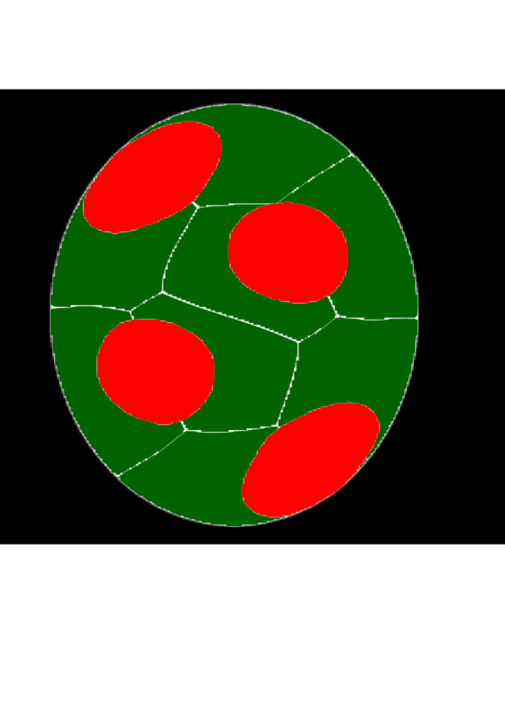
In this section, we consider the application of nuclear architecture reorganization system (2.7)-(2.10) to model drosophila nucleus with $8$ chromosomes and human nucleus with $46$ chromosomes. We present numerical simulations to explore the mechanisms underlying the reorganization process. The default computational domain is $\Omega=[-\pi,\pi)^{2}$ and $(2,2.9)$ is chosen to be the $x$ -diameter and $y$ -diameter of an elliptic nucleus which is located in the center of domain $\Omega$ . We use a Fourier spectral method in space with $256^{2}$ modes, coupled with the three time discretization schemes presented in the last section. When presenting the simulations results, nucleus is depicted in white, chromosome territories in green, and heterochromatin in red ( see Fig. 4).

First, we test the convergence rate for proposed linear scheme and weakly nonlinear schemes. Then we study the conventional architectures with affinity and without affinity. Finally, we explore the mechanisms underlying the reorganization process and the pattern formation of chromatin, e.g., the effect of nucleus size and shape and different phase parameters.

4.1 Convergence test

We first test the convergence rate for the linear scheme (3.37)-(3.40) and the weakly nonlinear scheme (3.48)-(3.52) with fixed nucleus. The phase parameters are set to be $\epsilon^{2}_{\phi}=0.01$ , $\epsilon^{2}_{\psi}=0.05$ , $\beta_{0}=\frac{5}{3}$ , $\beta_{\phi}=1$ , $\beta_{\psi}=\frac{2}{3}$ and $\gamma=0$ . The initial condition is chosen as the case of (b) in Fig. 4 with Affinity $>0$ . The reference solutions are obtained with a very small time step $\delta t=10^{-6}$ using the linear scheme (3.37)-(3.40). We plot $\max_{m=1}^{N}\|\phi_{m}-\phi_{m,Ref}\|_{L^{\infty}}$ and $\|\psi-\psi_{Ref}\|_{L^{\infty}}$ in Fig. 3. Second order convergence rate is observed for both schemes.

4.2 Affinity test and conventional architecture with fixed nucleus

We now demonstrate the conventional architecture for drosophila nucleus with $8$ chromosomes. The initial condition is given in Fig. 4 where an elliptic nucleus are generated by function $\phi_{0}(x,y)=\frac{1}{2}(1-\tanh(\frac{\sqrt{x^{2}+y^{2}/1.45^{2}}-2}{\sqrt{2}\epsilon}))$ . The $8$ chromosomes are initialized by tanh-like functions : $\frac{1}{2}[1-\tanh(\frac{r}{\sqrt{2}\epsilon})]$ with centers at $(0,2.5),(-1,1.4),(-0.3,-0.5),(1,-1),(0,0.6),(1,1.3),(0,-2.5),(-1,-0.8)$ . The $x$ -diameter and $y$ -diameter are $(0.2,0.4)$ for each elliptic nucleus. A smaller ellipse with $x$ -diameter and $y$ -diameter as $(0.05,0.1)$ in each chromosome is set to be heterochromatin territory. The affinity between heterochromatin and the nuclear envelope is controlled by the parameter $\gamma$ . A positive affinity value indicates a tethering of heterochromatin to LBR or lamin A/C on the nuclear envelope. To demonstrate that the conventional architecture is obtained with the positive affinity, we choose $\gamma=0.02$ and $\gamma=0$ and plot in Fig. 4 numerical results by using the weakly nonlinear scheme (3.22)-(3.25). We observe from Fig. 4 that heterochromatin domains are fused with adjacent heterochromatin. When affinity $=0$ heterochromatin accumulates at the territories between chromosomes. But there is no interaction with the region of the nuclear envelope. With a positive affinity, heterochromatin is observed to be distributed almost homogeneously along the nuclear envelope, indicating the formation of the conventional architecture. Our numerical simulations indicate that the affinity plays important roles in forming the conventional architecture, and that the expression of LBR and lamin A/C is essential to generate the conventional architecture. These numerical results are consistent with the experiment results in [29].

In Fig. 5, we plot the dynamics of mean volume of chromosome $\bar{V}(t)=\frac{\sum_{i=1}^{N}V_{m}}{N}$ and heterochromatin $\bar{v}(t)=\frac{\sum_{i=1}^{N}v_{m}}{N}$ . From Fig. 5, the volumes of chromosome and heterochromain are well preserved by using our weakly nonlinear schemes (3.22)-(3.25).

4.3 Inverted architecture and reorganization process

In this subsection, we study the architecture reorganization process with fixed nucleus. First, we examine whether the increase of heterochromatin conversion rate and the absence of affinity between the nuclear envelope and heterochromatin are necessary for the induction of the single hetero-cluster in the inverted architecture. We fix the heterochromatin conversion rate $\rho_{m}=\frac{v_{m}}{V_{m}}$ for $m=1,2,\cdots,N$ , and set $\gamma=0$ . From the first row of Fig. 6, it is observed that affinity between heterochromatin and nuclear envelope vanishes gradually. Finally, four clusters of heterochromatin are formed at $t=50$ when the conversion rates are fixed for all $m$ . We then examine the case with an increasing conversion rate $\rho_{m}(t)$ described by

\rho_{m}(t)=\rho_{m}(0)+\frac{\bar{\rho}_{m}t}{t+\alpha_{1}e^{-\alpha_{2}t}},

(4.67)

where $\alpha_{1}=150$ and $\alpha_{2}=0.3$ . In our simulations, we set the increased conversion rate to be $\bar{\rho}_{m}=\{(0.35,0.4,0.4,0.35,0.15,0.15,0.35,0.35)\}$ and $\bar{\rho}_{m}=\{(0.35,0.4,0.4,0.45,0.15,0.15,0.35,0.45)\}$ for the second and third rows in Fig. 6, and set the affinity parameter to be $\gamma=0$ . We observe from the second and third rows of Fig. 6 that a single cluster of heterochromatin is formed which implies the inverted architecture. Next we keep the affinity between the nuclear and the nuclear envelope unchanged at $\gamma=0.02$ , and increase the conversion rate $\rho_{m}$ for $m=1,2,\cdots,N$ . We observe from the fourth row of Fig. 6 that the affinity between nuclear envelope and heterochromatin are present all the time, and the heterochromatin grows on each chromosome territory gradually during architecture reorganization process.

The numerical simulations from Fig. 6 indicate that increase of heterochromatin conversion rate and the absence of affinity between nuclear envelope and heterochromatin are sufficient for the formation of the inverted architecture during the nuclear architecture reorganization process, which are with the previous results in [22].

4.4 Reduced nuclear size and the reorganization process

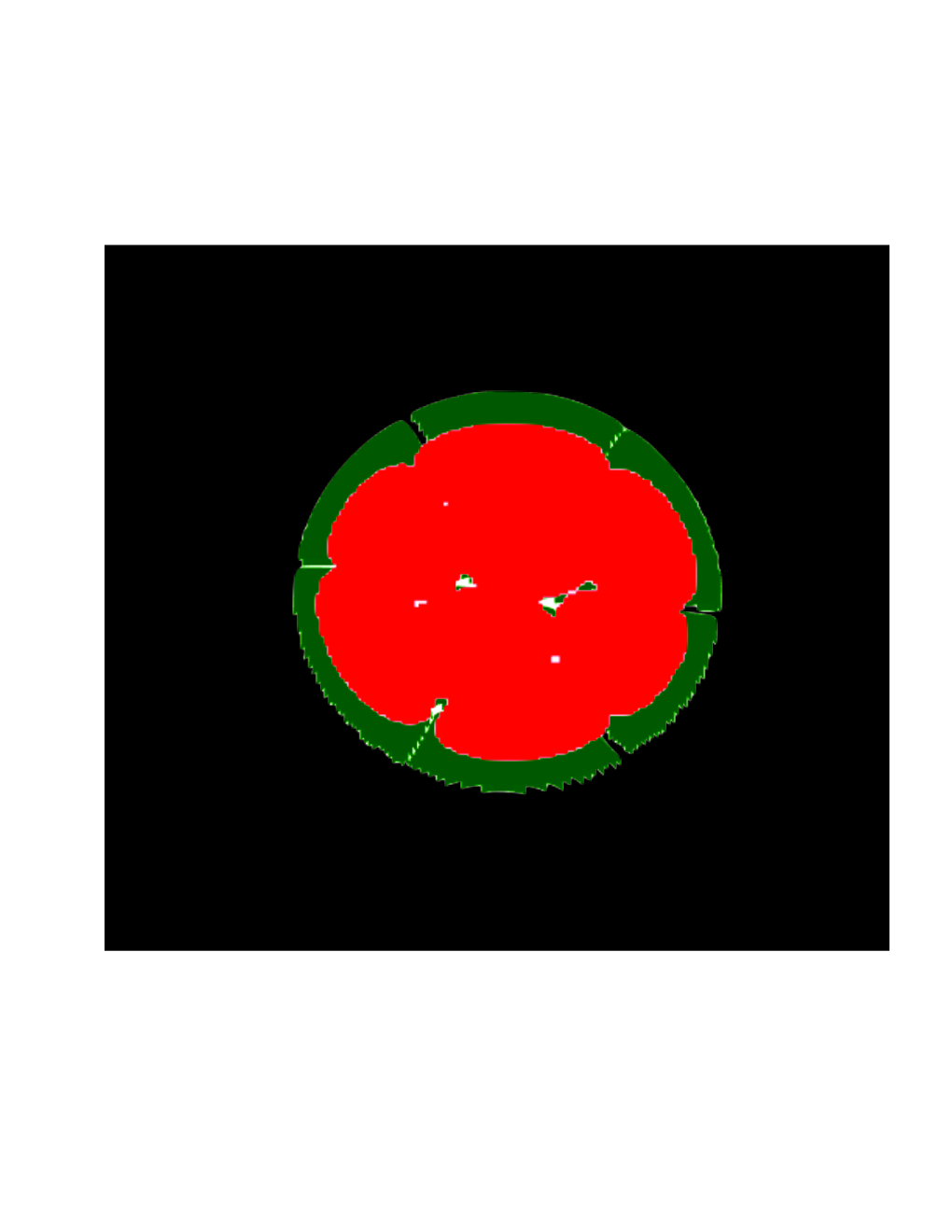
In this subsection, we focus on the architecture reorganization process with reduced nuclear shape, and assess whether the nuclear shape is an indispensable condition for the induction of a single cluster inverted architecture.

We introduce two sigmoid functions to describe the x-radius and y-radius of nuclear shape.

r_{x}(t)=r_{x}(0)+\frac{\bar{r}_{x}t}{t+\alpha_{1}e^{-\alpha_{2}t}};\;r_{y}(t)=r_{y}(0)+\frac{\bar{r}_{y}t}{t+\alpha_{3}e^{-\alpha_{4}t}},

(4.68)

where $\bar{r}_{x}$ and $\bar{r}_{y}$ are the decreasing rate of nuclear size and $\alpha_{1}$ , $\alpha_{2}$ , $\alpha_{3}$ and $\alpha_{4}$ are four positive constants which controls the decreasing scale with respect to time. We consider that the nucleus shape will decrease to be a circular or an elliptical shape with time evolution, and investigate how the nuclear size and shape influence the nuclear architecture reorganization process. The parameters of decreasing scale are $\alpha_{1}=\alpha_{3}=1$ and $\alpha_{2}=\alpha_{4}=0.01$ . Numerical results are computed by the linear scheme (3.48)-(3.52) with $\delta t=10^{-4}$ . We also increase the volume of each chromosome $V_{m}$ and volume of heterochromatin in each chromosome $v_{m}$ with time. Snapshots at $t=0,0.05,1,5$ are depicted for different nuclear pattern in Fig. 7. It is observed from Fig. 7 that both circular or elliptical shape will eventually achieve the one cluster inverted architecture. The second row of Fig. 7 displays chromosome territories of the first row. So the nuclear size or shape are not indispensable condition for the nuclear architecture reorganization process.

4.5 Inverted architecture reorganization for human beings

In the previous subsections, we only considered $8$ chromosomes for drosophila, and find that the deformation of nuclear size and shape are not sufficient conditions for the nuclear architecture conversion. The absence of both LBR and lamin A/C expression $\gamma=0$ and the increase of heterochromatin rate are indispensable for inverted nuclear architecture. Now we explore the nuclear architecture with $46$ chromosomes for human beings. We also compute the numerical results by using the linear scheme (3.37)-(3.40) with $\delta t=10^{-3}$ and examine the effect of affinity in Fig. 8. It is observed from Fig. 8 that heterochromatin is shown to be distributed along the nuclear envelope with $\gamma=0.02$ with $46$ chromosome. However the heterochromatin accumulates at the territories between chromosome instead of in the region of nuclear envelope with $\gamma=0$ . In Fig. 9, we decrease nuclear shape and eliminate the affinity of nuclear envelope, while increasing the heterochromatin conversion rate, and we observe that one cluster inverted architecture is formed at $t=2$ .

5 Concluding remarks

Specific features of nuclear architecture are closely related to the functional organization of the nucleus. Within nucleus, chromatin consists of two forms, heterochromatin and euchromatin. The conventional nuclear architecture is observed when heterochromatin is enriched at nuclear periphery, and it represents the primary structure in the majority of eukaryotic cells, including the rod cells of diurnal mammals. In contrast to this, the inverted nuclear architecture is observed when the heterochromatin is distributed at the center of the nucleus, which occurs in the rod cells of nocturnal mammals. The conventional architecture can transform into the inverted architecture during nuclear reorganization process.

We developed in this paper a new phase field model with Lagrange multipliers to simulate the nuclear architecture reorganization process. Introducing Lagrange multipliers enables us to preserve the specific physical and geometrical constraints for the biological events. We developed several efficient time discretization schemes for the constrained gradient system. One is a full linear scheme which can only preserve volume constrains with second order accuracy, but it is very easy to solve. The other two are weakly nonlinear scheme which can exactly preserve non-local constraints, and one of them is also unconditionally energy stable. The price we pay for the exact preservation of geometric constraints is that we need to solve a nonlinear algebraic system for the Lagrange multipliers, which can be solved at negligible cost but may require the time step to be sufficiently small. These time discretization schemes can be used with any consistent Galerkin type discretization in space.

We presented several simulations using our proposed schemes for drosophila and human beings with $8$ chromosomes and $46$ chromosomes. Our results indicate that the increase of heterochromatin conversion rate and the absence of affinity between nuclear envelope and heterochromatin are sufficient for the formation of the inverted architecture during the nuclear architecture reorganization process, while nuclear size and shape are not indispensable for the formation of the single hetero-cluster inverted architecture.

References

[1] Bruce Alberts, Dennis Bray, Karen Hopkin, Alexander D Johnson, Julian Lewis, Martin Raff, Keith Roberts, and Peter Walter. Essential cell biology. Garland Science, 2015.
[2] Long Qing Chen and Jie Shen. Applications of semi-implicit fourier-spectral method to phase field equations. Computer Physics Communications, 108(2-3):147–158, 1998.
[3] Qing Cheng, Chun Liu, and Jie Shen. A new interface capturing method for allen-cahn type equations based on a flow dynamic approach in lagrangian coordinates, i. one-dimensional case. Journal of Computational Physics, 419:109509, 2020.
[4] Qing Cheng and Jie Shen. Multiple scalar auxiliary variable (msav) approach and its application to the phase-field vesicle membrane model. SIAM Journal on Scientific Computing, 40(6):A3982–A4006, 2018.
[5] Qing Cheng and Jie Shen. Global constraints preserving sav schemes for gradient flows. SIAM Journal On Scientific Computing, 2019.
[6] Thomas Cremer and Christoph Cremer. Chromosome territories, nuclear architecture and gene regulation in mammalian cells. Nature reviews genetics, 2(4):292–301, 2001.
[7] Thomas Cremer and Marion Cremer. Chromosome territories. Cold Spring Harbor perspectives in biology, 2(3):a003889, 2010.
[8] Thomas Cremer, Marion Cremer, Steffen Dietzel, Stefan Müller, Irina Solovei, and Stanislav Fakan. Chromosome territories–a functional nuclear landscape. Current opinion in cell biology, 18(3):307–316, 2006.
[9] Qiang Du and Fanghua Lin. Numerical approximations of a norm-preserving gradient flow and applications to an optimal partition problem. Nonlinearity, 22(1):67–83, December 2008.
[10] Qiang Du, Chun Liu, Rolf Ryham, and Xiaoqiang Wang. Energetic variational approaches in modeling vesicle and fluid interactions. Physica D: Nonlinear Phenomena, 238(9):923–930, May 2009.
[11] Qiang Du, Chun Liu, and Xiaoqiang Wang. Simulating the deformation of vesicle membranes under elastic bending energy in three dimensions. Journal of computational physics, 212(2):757–777, March 2006.
[12] Fabian Erdel and Karsten Rippe. Formation of chromatin subcompartments by phase separation. Biophysical journal, 114(10):2262–2270, 2018.
[13] Xiaobing Feng and Andreas Prohl. Numerical analysis of the allen-cahn equation and approximation for mean curvature flows. Numerische Mathematik, 94(1):33–65, 2003.
[14] Zhen Guan, John Lowengrub, and Cheng Wang. Convergence analysis for second-order accurate schemes for the periodic nonlocal allen-cahn and cahn-hilliard equations. Mathematical Methods in the Applied Sciences, 40(18):6836–6863, 2017.
[15] Zhen Guan, John S Lowengrub, Cheng Wang, and Steven M Wise. Second order convex splitting schemes for periodic nonlocal cahn–hilliard and allen–cahn equations. Journal of Computational Physics, 277:48–71, 2014.
[16] Gamze Gürsoy, Yun Xu, Amy L Kenter, and Jie Liang. Spatial confinement is a major determinant of the folding landscape of human chromosomes. Nucleic acids research, 42(13):8223–8230, 2014.
[17] Gamze Gürsoy, Yun Xu, Amy L Kenter, and Jie Liang. Computational construction of 3d chromatin ensembles and prediction of functional interactions of alpha-globin locus from 5c data. Nucleic acids research, 45(20):11547–11558, 2017.
[18] Gamze Gürsoy, Yun Xu, and Jie Liang. Spatial organization of the budding yeast genome in the cell nucleus and identification of specific chromatin interactions from multi-chromosome constrained chromatin model. PLoS computational biology, 13(7):e1005658, 2017.
[19] Xiaobo Jing and Qi Wang. Linear second order energy stable schemes for phase field crystal growth models with nonlocal constraints. Comput. Math. Appl., 79(3):764–788, 2020.
[20] Nicholas Allen Kinney, Igor V Sharakhov, and Alexey V Onufriev. Chromosome–nuclear envelope attachments affect interphase chromosome territories and entanglement. Epigenetics & chromatin, 11(1):1–18, 2018.
[21] Rabia Laghmach, Michele Di Pierro, and Davit A Potoyan. Mesoscale liquid model of chromatin recapitulates nuclear order of eukaryotes. Biophysical journal, 118(9):2130–2140, 2020.
[22] S Seirin Lee, S Tashiro, A Awazu, and R Kobayashi. A new application of the phase-field method for understanding the mechanisms of nuclear architecture reorganization. Journal of mathematical biology, 74(1-2):333–354, 2017.
[23] Chun Liu and Jie Shen. A phase field model for the mixture of two incompressible fluids and its approximation by a fourier-spectral method. Physica D: Nonlinear Phenomena, 179(3-4):211–228, 2003.
[24] Jonas Paulsen, Monika Sekelja, Anja R Oldenburg, Alice Barateau, Nolwenn Briand, Erwan Delbarre, Akshay Shah, Anita L Sørensen, Corinne Vigouroux, Brigitte Buendia, et al. Chrom3d: three-dimensional genome modeling from hi-c and nuclear lamin-genome contacts. Genome biology, 18(1):1–15, 2017.
[25] Alan Perez-Rathke, Qiu Sun, Boshen Wang, Valentina Boeva, Zhifeng Shao, and Jie Liang. Chromatix: computing the functional landscape of many-body chromatin interactions in transcriptionally active loci from deconvolved single cells. Genome biology, 21(1):1–17, 2020.
[26] Nikolas Provatas and Ken Elder. Phase-field methods in materials science and engineering. John Wiley & Sons, 2011.
[27] Sungrim Seirin-Lee. Role of domain in pattern formation. Development, growth & differentiation, 59(5):396–404, 2017.
[28] Irina Solovei, Moritz Kreysing, Christian Lanctôt, Süleyman Kösem, Leo Peichl, Thomas Cremer, Jochen Guck, and Boris Joffe. Nuclear architecture of rod photoreceptor cells adapts to vision in mammalian evolution. Cell, 137(2):356–368, 2009.
[29] Irina Solovei, Audrey S Wang, Katharina Thanisch, Christine S Schmidt, Stefan Krebs, Monika Zwerger, Tatiana V Cohen, Didier Devys, Roland Foisner, Leo Peichl, et al. Lbr and lamin a/c sequentially tether peripheral heterochromatin and inversely regulate differentiation. Cell, 152(3):584–598, 2013.
[30] Amy R Strom, Alexander V Emelyanov, Mustafa Mir, Dmitry V Fyodorov, Xavier Darzacq, and Gary H Karpen. Phase separation drives heterochromatin domain formation. Nature, 547(7662):241–245, 2017.
[31] Qiu Sun, Alan Perez-Rathke, Daniel M Czajkowsky, Zhifeng Shao, and Jie Liang. High-resolution single-cell 3d-models of chromatin ensembles during drosophila embryogenesis. Nature communications, 12(1):1–12, 2021.
[32] Shouwen Sun, Jun Li, Jia Zhao, and Qi Wang. Structure-preserving numerical approximations to a non-isothermal hydrodynamic model of binary fluid flows. Journal of Scientific Computing, 83:1–43, 2020.
[33] Bas Van Steensel and Andrew S Belmont. Lamina-associated domains: links with chromosome architecture, heterochromatin, and gene repression. Cell, 169(5):780–791, 2017.
[34] Xiaoqiang Wang, Lili Ju, and Qiang Du. Efficient and stable exponential time differencing runge–kutta methods for phase field elastic bending energy models. Journal of Computational Physics, 316:21–38, 2016.
[35] Xiaofeng Yang. Numerical approximations of the navier–stokes equation coupled with volume-conserved multi-phase-field vesicles system: fully-decoupled, linear, unconditionally energy stable and second-order time-accurate numerical scheme. Computer Methods in Applied Mechanics and Engineering, 375:113600, 2021.
[36] Xiaofeng Yang and Lili Ju. Efficient linear schemes with unconditional energy stability for the phase field elastic bending energy model. Computer Methods in Applied Mechanics and Engineering, 315:691–712, 2017.