All-optical quantum simulation of ultrastrong optomechanics
Abstract
The observation of single-photon optomechanical effects is a desired task in cavity optomechanics. However, the realization of ultrastrong optomechanical interaction remains a big challenge. Here, we present an all-optical scheme to simulate ultrastrong optomechanical coupling based on a Fredkin-type interaction, which consists of two exchange-coupled modes with the coupling strength depending on the photon number in another controller mode. This coupling enhancement is assisted by the displacement amplification according to the physical idea of the Bogoliubov approximation, which is realized by utilizing a strong driving to pump one of the two exchanging modes. Our numerical simulations demonstrate that the enhanced optomechanical coupling can enter the single-photon strong-coupling and even ultrastrong-coupling regimes. We also show the creation of macroscopic quantum superposed states and the implementation of a weak-to-strong transition for quantum measurement in this system. This work will pave the way to quantum simulation of single-photon optomechanical effects with current experimental platforms.
I Introduction
The recent developments in cavity optomechanics Kippenberg2008rev; Aspelmeyer2012rev; Aspelmeyer2014 facilitate the study of radiation-pressure interactions between electromagnetic fields and mechanical vibrations, especially at the single-photon level Rabl2011; Nunnenkamp2011; Liao2012; Liao2013; Liao2013PRA; Hong2013; Xu2013; Tang2014; Marshall2003; Liao2016. The coherent nonlinear optomechanical interaction is the physical origin of various interesting physical effects, such as the appearance of phonon sidebands in the cavity emission spectrum Nunnenkamp2011; Liao2012, photon blockade effect induced by the moving boundary Rabl2011; Liao2013; Liao2013PRA; Xu2013, and the generation of macroscopic quantum superposition Marshall2003; Liao2016. In particular, this provides a good platform for investigating some fundamental issues in quantum mechanics, for example, the quantum measurement problem, a puzzle that has not yet been completely resolved Neumann2018. Hence, how to efficiently manipulate the optomechanical interactions at the single-photon level has become one of the most interesting research topics in this field. However, it has remained a big challenge to observe single-photon optomechanical effects with current experimental techniques. This is because the magnitude of the optomechanical coupling associated with a single photon is too weak to enter the single-photon strong-coupling regime.
By far, several schemes have been proposed to amplify the single-photon optomechanical effects Brennecke2008; Xuereb2012; Rimberg2014; Heikkila2014; Pirkkalainen2015; Liao2014; Liao2015; Lue2015; Lemonde2016; Li2016; Wang2017; Liao2020, such as the enhancement of the optomechanical coupling with a collective density excitation of the Bose-Einstein condensate Brennecke2008 or collective modes Xuereb2012, the resonant enhancement induced by either coupling Liao2014; Liao2016 or cavity-frequency Liao2015 modulation, the utilization of the strong nonlinearity in the Josephson junctions Rimberg2014; Heikkila2014; Pirkkalainen2015, the effective coupling enhancement induced by either the squeezing transformation Lue2015; Lemonde2016; Li2016 or the displacement transformation Liao2020, and the utilizing of delayed quantum feedback Wang2017. Nevertheless, there are no reports on the demonstrations of single-photon optomechanical effects. Inspired by the motivation of simulating the experimentally inaccessible physical effects with accessible physical system Nori2014, in this paper we propose an all-optical scheme to implement a quantum simulation of a tunable optomechanical interaction, which can enter single-photon strong-coupling and ultrastrong-coupling regimes Hu2015. In this way, we are able to generate distinct macroscopic superposed states with this enhanced optomechanical coupling. As an important feature of this system, the obtained optomechanical interaction can be controlled on demand by choosing proper drivings. Therefore, by adjusting the interaction strength from weak to strong, this system is used to exhibit the quantum measurement transition from the weak value to the expectation value Aharonov1998; Pan2020.
The rest of this paper is organized as follows. In Sec. II we introduce the physical model and present the Hamiltonians. In Sec. III we derive the approximate optomechanical Hamiltonian and evaluate the validity of the approximate Hamiltonian. In Secs. IV, V, and VI we study the generation of the Schrödinger cat states in mode , the implementation of the weak-to-strong transition of quantum measurement, and the photon blockade effect in mode , respectively. We present a discussion on the experimental implementation of this scheme in Sec. VII and summarize this work in Sec. VIII.
II Physical model
We consider an all-optical platform to simulate an ultrastrong optomechanical interaction based on a Fredkin-type interaction Milburn1989; Patel2016; Gao2019Nature, which consists of three optical modes described by the annihilation (creation) operators , , and , with the corresponding resonance frequencies , , and . Here the Fredkin interaction takes the form of a conditional two-mode exchange coupling (a beam-splitter-type coupling between modes and possessing a coupling strength depending on the photon numbers in mode ). Mode is driven by a strong monochromatic laser field with amplitude and frequency . In a rotating frame with respect to , the Hamiltonian of the system reads
| (1) | |||||
where and are the detunings and is the coupling strength of the Fredkin interaction. In Eq. (1) we neglect the counterrotating terms , where and denote the norm of the operators and , respectively.
To include the dissipation of the system, we assume that the three optical modes are coupled to three individual Markovian reservoirs. Then the evolution of the system can be described by the quantum master equation
| (2) |
where is the standard Lindblad superoperator. The parameters , , and , , are, respectively, the damping rate and the environment thermal excitation occupation of modes , , . Here, we consider the general case where the Markovian reservoirs are at finite temperatures. Though our scheme is based on three optical modes, it is universal to other bosonic systems, in which the effect of temperature may appear. Therefore, we include this effect in our simulation scheme.
III The generalized optomechanical Hamiltonian
In this section, we derive the generalized optomechanical Hamiltonian (approximate Hamiltonian) and evaluate the validity of the approximate Hamiltonian.
III.1 Derivation of the approximate Hamiltonian
We first sketch the inspiration concerning this coupling enhancement. Under the strong driving, the average photon number in mode is large and then the operator can be expressed as a sum of its average value and quantum fluctuation: . Consequently, the Fredkin interaction becomes , which can be reduced to an amplified optomechanical interaction (the target term) by discarding the first term under proper conditions. The rigorous derivation is performed by making the transformation
| (3) |
where is the displacement operator, with the displacement amplitude . In the displacement representation, the quantum master equation of the system takes the form
| (4) |
where we introduce the displaced Hamiltonian
| (5) | |||||
with the transient displacement amplitude determined by . The steady-state displacement amplitude is given by , which can be tuned by selecting driving parameters and . To investigate the ultrastrong optomechanics, hereafter we consider a few excitations in modes and . Under the parameter conditions and , with the maximal dominant excitation numbers involved in mode , the term can be ignored by the rotating-wave approximation (RWA) and mode decouples from modes and . Apart from the decoupling term , a generalized optomechanical Hamiltonian is obtained as
| (6) |
where the interaction term takes the form as the product of the photon-number operator of mode and the rotated quadrature operator of mode (playing the role of the mechanical mode in typical optomechanical systems). Here the tunable single-photon optomechanical-coupling strength can be largely enhanced by using proper driving, and the phase angle is tunable by choosing the proper driving phase in .
III.2 Evaluation of the validity of the approximate Hamiltonian
The validity of the approximate Hamiltonian can be evaluated by checking the fidelity between the exact and approximate states, which are governed by the full Hamiltonian and the approximate Hamiltonian , respectively. To this end, we need to calculate the analytical results of the approximate and exact states for the system at time .
III.2.1 The analytical state determined by the approximate Hamiltonian
To obtain the analytical state of the system at time , we need to diagonalize the approximate Hamiltonian . This can be done by introducing the displacement operator , with the photon-number dependent displacement amplitude
| (7) |
where is the -photon-dependent displacement amplitude. In addition, we consider the phase angle . Then the approximate Hamiltonian can be diagonalized as
| (8) |
Therefore, the analytical approximate state of the system at time can be obtained as
| (9) | |||||
where we introduce the displacement amplitudes
| (10a) | ||||
| (10b) | ||||
and the phase
| (11) |
III.2.2 The analytical state determined by the exact Hamiltonian
The exact state of the system at time can also be obtained analytically by diagonalizing the exact Hamiltonian . To this end, we introduce three transformation operators , , and based on the photon-number dependent mixing angle
| (12) |
and displacement amplitudes
| (13a) | ||||
| (13b) | ||||
with
| (14a) | ||||
Here these -photon dependent variables , , , , and are defined by
| (15a) | ||||
| (15b) | ||||
| (15c) | ||||
| (15d) | ||||
| (15e) | ||||
By performing these transformations, the Hamiltonian can be diagonalized as
| (16) | |||||
Based on Eq. (16), the exact state of the system at time corresponding to the initial state can be obtained as
| (17) | |||||
Here, we introduce the displacement amplitudes
| (18a) | ||||
| (18b) | ||||
and the phase
| (19) | |||||

III.2.3 The fidelity between the approximate state and the exact state
Based on the expressions of the exact and approximate states, we can calculate the fidelity between the exact state and the approximate state as
| (20) | |||||
Without loss of generality, here we assume the initial state of the system, with and coherent states. Note that the initial time here corresponds to the time when the system reaches its steady state. In addition, we include mode in in our simulations. This is because our simulations are performed for the total system, though mode decouples with modes and . In particular, we first consider the closed-system case for avoiding the crosstalk from the system dissipation. In Fig. 1(a) we display the fidelity given by Eq. (20) as a function of the evolution time when and , , and . In addition, we use the scaled parameters in our numerical simulations for indicating the universality of our scheme. These parameters are within the reach of current experimental conditions. In Fig. 1(a), we find that a higher fidelity can be obtained for a larger value of the ratio of , which coincides with the parameter conditions for the RWA. To show that the fidelity is high in a wide parameter space, we plot the fidelity at time (the time for generation of the cat state in mode ) as a function of the two tunable parameters and in Fig. 1(b). Here the fidelity is high in our selected parameter space and hence the approximate Hamiltonian (6) can properly describe the system. Note that the term commutates with other terms in the Hamiltonian, and hence the fidelity is independent of .

We also investigate the influence of the system dissipation on the fidelity. In the open-system case, the evolution of the exact and approximate states are governed by the exact and approximate quantum master equations, respectively. The latter takes the same form as the exact quantum master equation (4) under the replacement . In addition, for calculational convenience we introduce a parameter into the term in the displaced Hamiltonian by replacing ; then the exact and approximate equations of motion for the density-matrix elements can be expressed in a unified form. The values of and correspond to the exact and approximate solution cases, respectively. For convenience, we express the density matrix of the full system in the Fock-state space as
| (21) |
with
| (22) |
In our numerical simulations, the appropriate truncation dimension of the summations in Eq. (21) needs to be chosen and Eq. (48) also follows the same convention. To solve the equations of motion for these density-matrix elements, we assume that the initial state of the system is either with coherent states and or ; then the corresponding initial conditions are given, respectively by
| (23a) | ||||
| (23b) | ||||
With Eq. (23), the fidelity between the exact and approximate density matrices and (corresponding to and , respectively) is given by
| (24) |
In the presence of dissipation, the relaxation time is of the order of , which is much shorter than the time scale due to . This means that our scheme works in the weak-coupling regime for the initial interaction determined by the term . To show the feasibility of our method, in Fig. 2 we plot the fidelity given by Eq. (24) as a function of the evolution time in the open-system case. In principle, the initial state of the system can be chosen arbitrarily, whereas to save computational resources, we select the initial state of the system as either or . Meanwhile, for realization of the ultrastrong-coupling regime, a proper displacement amplitude is considered so that the relation can be satisfied. Here we find that a smaller value of the ratio corresponds to a higher fidelity, which confirms our analysis for the parameter conditions of the RWA. In addition, the fidelity exhibits some oscillations and then reaches gradually a stationary value due to the system dissipation. For a given , corresponding to the higher decay rate of the system, the faster the fidelity decays to a stationary value. However, from Fig. 2 we see that the values of the fidelities increase gradually over time until they are equal to 1. The physical origin can be seen from the approximate Hamiltonian and the exact Hamiltonian , in which mode is not driven but couples to a zero-temperature reservoir. Therefore, the average photon number in mode becomes zero in the long-time limit, namely, obtaining the steady state of mode . This vacuum state of mode can lead to the disappearance of the terms and ; then both modes and are reduced to free-cavity modes connected with individual zero-temperature reservoirs. Hence the corresponding steady states of modes and are and , respectively. As a result, the fidelity between exact and approximate states is one in the long-time limit.
III.2.4 Parameter space analysis
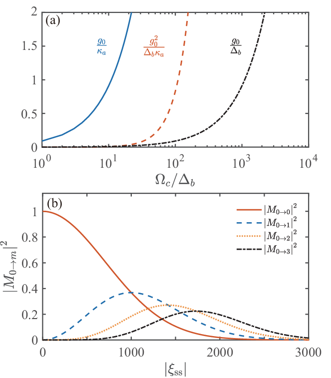
To clearly see the coupling enhancement in this system, we present an analysis of the parameter space of the enhanced optomechanical interaction. Concretely, we analyze three ratios, , , and , which have important physical meaning in optomechanical systems Aspelmeyer2014. In optomechanics, corresponds to the single-photon strong-coupling regime, in which the mechanical quantum fluctuation induced by a single photon can be resolved from the zero-point fluctuation of the mechanical mode Ludwig2008. The relation represents the strong-dispersive-coupling condition which ensures that the energy nonharmonicity induced by the Kerr nonlinearity can be resolved from the cavity emission spectrum of mode in the case of Rabl2011. In addition, the relation denotes the deep-strong-coupling condition which means that the displacement of mode forced by a single photon can be distinguished from the vacuum state of mode Marshall2003. In Fig. 3(a) we show the ratios , , and as functions of the driving amplitude . Here we can see that for a large driving amplitude, these three ratios can be larger than 1, which means that single-photon optomechanical effects can be observed in this system.
The enhanced optomechanical interaction can also be witnessed by analyzing the transition suppression effect. We consider the transitions between the states and , where defines the single-photon displaced number state with the single-photon displacement depending on [see Eq. (77) for the expression of ]. The transition probability, called the Franck-Condon (FC) factor Franck1925; Condon1926; Leturcq2009, is proportional to the square of the overlap between the ground state and the displaced number states , and it takes the form
| (25) |
Figure 3(b) shows the FC factors as a function of the enhanced factor , from which we see that the ground-state-to-ground-state transition, determined by , is exponentially suppressed for a large . However, the peak values of other FC factors are located at a larger for a larger . Furthermore, the peak values of these FC factors decrease gradually as the excited number increases.
IV Macroscopic quantum superposition
In this section we show how to generate the Schrödinger cat states for the mechanical-like mode Marshall2003 in terms of the approximate Hamiltonian and the exact Hamiltonian . We also study the influence of the system dissipation on the cat-state generation.
IV.1 Cat-state generation based on the approximate Hamiltonian
In a rotating frame with respect to , the approximate Hamiltonian becomes
| (26) |
The unitary evolution operator associated with is given by
| (27) |
where is the unitary evolution operator relevant to and it is governed by the equation of motion with initial condition given by . Its formal solution can be written as , where denotes the time-ordering operator. According to the Magnus proposal, can be obtained as
To generate the cat states, we choose the initial state of the system as
| (29) |
where we select the initial state of mode as to save computational resources. It should be pointed out that the initial state of mode in the original representation is a coherent state with the coherent amplitude given by . Therefore, according to the unitary evolution operator (27), the state of the system at time can be obtained as
| (30) |
where we introduce the phase
| (31) |
and the displacement amplitude
| (32) |
From Eq. (32) we see that the maximal displacement is obtained at time for natural numbers . To see the displacement effect in mode induced by a single photon, we calculate the average excitation in mode based on the approximate Hamiltonian . As shown by the markers in Fig. 4(a), a larger will lead to a larger maximal displacement, and the dissipation will decrease the maximal value of the displacement. In particular, we plot the average excitation number at the cat-state generation time as a function of [see the markers in the inset of Fig. 4(a)]. Here we can see that the peak value of the displacement could be larger than the zero-point fluctuations of mode in the presence of dissipation.


To generate the macroscopic quantum superposed states of mode , we measure the state of modes and with the basis states . In terms of the basis states , the state in Eq. (30) can be reexpressed as
| (33) | |||||
If we perform a measurement on the system with the basis states , mode will collapse into two analytical cat states
| (34) |
where the normalization constants are defined by
| (35) |
The measuring probabilities corresponding to states are given by
| (36) |
Equation (36) indicates that, for a sufficiently large displacement , the measurement probabilities will approach due to . In Fig. 4(b) we use the markers to denote the probabilities as functions of the evolution time , which shows that and have similar oscillation envelops. In addition, the inset in Fig. 4(b) indicates that the oscillation amplitude is almost negligible and the probabilities in the intermediate duration around the detection time , which confirms our analysis of the measurement probabilities [denoted by the markers in Fig. 4(b)].
To see the quantum interference and coherence effects in the generated Schrödinger cat states, we now calculate the Wigner function. For a single-mode system described by the density matrix , the Wigner function is defined by Barnettbook
| (37) |
where is the displacement operator. Corresponding to the approximate analytical cat states in Eq. (34), the Wigner functions can be obtained by substituting the density matrices into Eq. (37) as
| (38) | |||||
with the normalization constants given by Eq. (35). In Figs. 5(a) and 5(b) we plot the Wigner functions for the approximate analytical cat states at the detection time when the dimensionless displacement amplitude and , respectively. Here we only plot the Wigner function for concision. By comparison, we see that the magnitude of can enhance the distinguishability between the two coherent states and and the visibility of the interference fringes (in the region between the two peaks). Therefore the enhanced optomechanical coupling realized by our scheme is useful to create macroscopically distinct superposition states in mode .

An alternative approach to observe the quantum coherence and inference effects in the generated cat states is to investigate the probability distribution of the rotated quadrature operator. For the rotated quadrature operator
| (39) |
we can denote its eigenstate by : Milburnbook. Considering the states , we obtain the probability distribution of the rotated quadrature operator as
| (40) | |||||
with the inner product and given by
where are the Hermite polynomials.

In Fig. 5(c) we plot the probability distributions for the state . Here we take the rotated angle ; the quadrature direction is, in this case, perpendicular to the link line between the two main peaks. Whenever the two coherent states are projected onto this quadrature, the probability distributions will overlap exactly, which will make the interference maximum. As shown in Fig. 5(c), the larger can cause a stronger oscillation in the probability distributions corresponding to the generated cat states. Note that the probability distributions are much easier to detect than the Wigner functions because the quadrature operators only need to be measured at a given rotating angle.
IV.2 Cat-state generation based on the exact Hamiltonian
It should be pointed out that the generated cat states can also be calculated based on the exact Hamiltonian . For the given initial state , the exact state at time can be obtained as
| (42) |
by using the result given in Eq. (17), where , , and are given by Eqs. (18) and (19) at , respectively. In terms of the basis states and Eq. (42), the exact analytical cat states for mode after the measurement of modes and can be obtained as
| (43) |
where the normalization constants are defined by
| (44) |
The corresponding probabilities for the measured states are given by
| (45) |
Based on the above discussion, in Fig. 4(a) we also plot the average excitation number of mode as a function of the evolution time when the amplification factor takes different values: , , and [see the solid curves in Fig. 4(a)]. The solid curves in the inset of Fig. 4(a) show the average excitation at time as a function of in both closed- and open-system cases. In addition, the time dependence of the probabilities is plotted by the solid curves in Fig. 4(b). We see from Fig. 4 that the results based on the approximate Hamiltonian and the exact Hamiltonian match well, which further confirms the validity of the approximate Hamiltonian .

Similar to the preceding discussion, by using Eq. (37), we can obtain the Winger functions of the exact analytical cat states as
| (46) | |||||
Using the relation given in Eq. (IV.1), the probability distributions of the rotated quadrature operator for can be obtained as
Figures. 5(d)5(f) plot the Wigner function and the probability distribution of the rotated quadrature operator at and , which show good agreement with the results of the approximate analytical cat states .
IV.3 Cat-state generation in the open-system case
In order to confirm the scheme of the state generation in an ideal case, we consider the state generation based on the exact Hamiltonian and including the system dissipation. Therefore, we need to numerically solve the quantum master equation and to measure modes and at time in the states ; then mode will collapse into two density matrices. To solve the evolution of the system, we express the density matrix in the Fock-state representation as
| (48) |
The density matrix can be obtained by solving the equations of motion for the density matrix elements. After the measurement, the reduced density matrices of mode become
| (49) | |||||
where we introduce the variables
| (50) |
and the measurement probabilities
| (51) |
The fidelities between the generated cat states and the analytical target states are calculated by
| (52) |
Here we choose in our simulations so that ; then the two states and can be well distinguished in phase space at . In Fig. 6(a) we display the fidelities at the detection time as functions of the decay rates and , respectively. Here we can see that the influence of the decay of mode on the fidelities is more serious than that of mode . In addition, we show versus the average thermal occupation in Fig. 6(b). As expected, the fidelities are attenuated gradually with the increase of .
Using Eq. (37), the Wigner functions for the states can be calculated as
| (53) |
By calculating the matrix elements of the displacement operator in the number-state representation
| (54) |
with and the displacement operator and the associated Laguerre polynominals, repectively, then we can obtain the values of the Wigner functions .
To see the influence of the system dissipation on the Wigner functions, we show in Fig. 7 of the generated cat states [Figs. 7(a)7(d)] and [Figs. 7(e)7(h)] in mode as a function of a complex variable when the decay rate takes different values. Obviously, the superposed coherent states with distinguishable superposition components and quantum interference pattern can be observed clearly from the Wigner functions. However, the increase of the decay rate attenuates the interference pattern gradually (the region between the two peaks) and the main peak corresponding to the coherent component is also reduced gradually.

As the effective frequency of mode is replaced by , acting as the frequency of a mechanical-like resonator, it makes sense to investigate the effect of the thermal occupation number in mode on the generation of the cat states. In Fig. 8 we display the Wigner functions of the generated cat states at different values of . We see that with the increase of , the quantum interference gradually decreases and even ultimately disappears.
Similarly to the closed-system case, from the probability distributions , we can observe the influence of the dissipation on quantum interference. For the numerical cat states , the probability distributions can be obtained as
| (55) |
In Fig. 9 we show for the density matrices as a function of when and take different values. It can be seen that the oscillation amplitude of the probability distributions decrease gradually with the increase of the decay rates and thermal occupation number. This means that the dissipation of the system will wash out the quantum coherence in the cat states.
V Weak-to-strong transition of quantum measurement
The tunable optomechanical interaction is an ideal platform to show the weak-to-strong transition in quantum measurement. Concretely, we choose modes and as the measured system and measuring pointer, respectively Pepper2012. Consider the preselection initial state ; then the state of the system at time becomes . In what follows, we perform a projective measurement by postselecting mode in the final state , where is the postselection angle. To obtain the measurement information of the system, we measure the operator in both the weak- and strong-coupling cases. According to the definition of a weak value Aharonov1998; Kofman2012; Dressel2014, we have in the weak-measurement regime. However, in the strong-measurement regime, we gain the expectation value as . Performing the projective measurement of state in the final state , the normalized final state of the pointer becomes
| (56) |
where the factor determines the transition from weak to strong measurements.
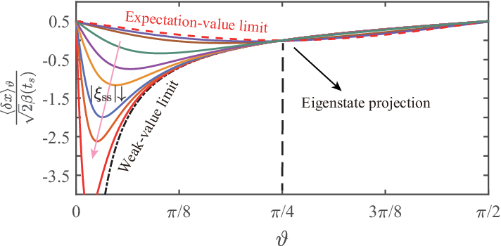
The above two cases of measurement outcomes can be unified by the pointer shift relative to that of the vacuum state , which is defined as , with the dimensionless position operator defined as . Substitution of Eq. (56) into yields
| (57) |
Here we choose the detection time and the phase angle . Then we have with . In the weak-coupling regime , the factor in Eq. (57) approaches 1 at proper parameter conditions. We then obtain , which is consistent with the weak value of the measured photon number operator. In the strong-coupling regime , we find , corresponding to the expectation value. In Fig. 10 we display the pointer shift as a function of the postselection angle at different values of . It can be found that when is small, we can appropriately choose the postselection angle such that the pre- and postselected states are nearly orthogonal. Then there exists a surprising weak-value amplification phenomenon Aharonov1998; Kofman2012; Dressel2014. In particular, the weak value is equal to the expectation value at , indicating an eigenstate projection. Moreover, by tuning the enhanced optomechanical coupling strength , the pointer shift will show the transition of the measurement outcome from a weak value to an expectation value Pan2020.
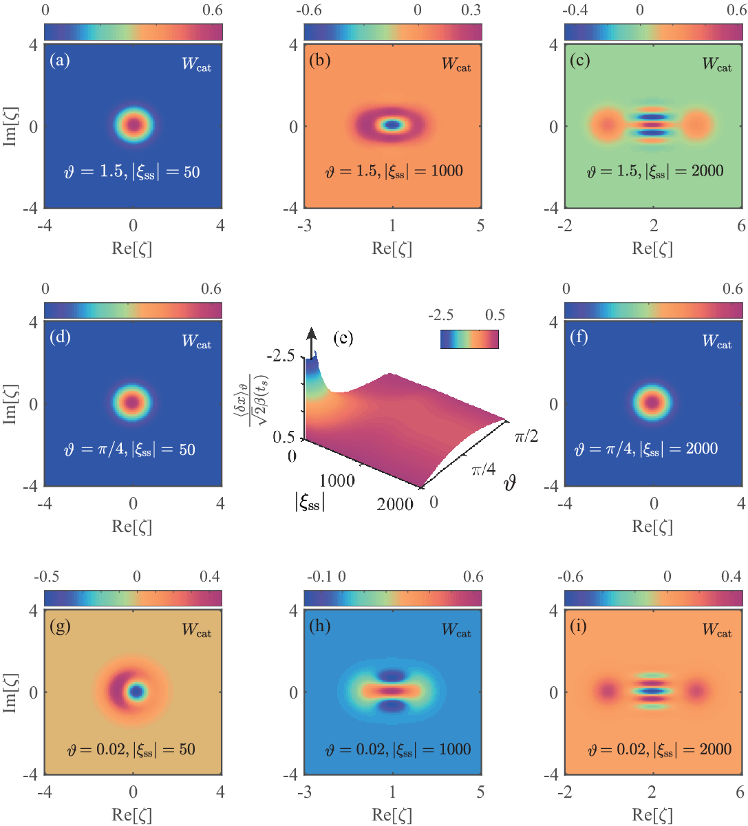
To clearly see the weak-to-strong transition of quantum measurement, we plot the Wigner functions of the pointer state in the full parameter space for the measurement regime in Fig. 11. Figures 11(a), 11(d), and 11(g) correspond to the weak-measurement regime with and post-selection angles , , and , respectively. The three angles represent, respectively, nearly orthogonal, eigenstate projection, and nearly parallel pre- and postselected states. As shown in Fig. 11(g), for the postselection angle , the postselection state is nearly orthogonal to the preselected state Then a remarkable weak-value amplification can be observed even in the weak-measurement coupling regime with . Figures 11(b) and 11(h) represent the intermediate-measurement regime at post-selection angles and , from which we can still see a distinct overlap between the two superposed coherent states. In Figs. 11(c) and 11(i), however, the two coherent states can have a negligible overlap as the increase of the steady-state displacement amplitude . Therefore, the two well-separated coherent states can be observed in phase space. In Figs. 11(d) and 11(f) we see there is only one peak located at the origin of the phase space. This is because corresponds to the eigenstate projection, which can cause the superposition coefficient of the coherent state in the cat state to be 0. Then the cat state reduces to the ground state of mode . Hence, we cannot observe the displacement of the cat state for all coupling strengths.
VI Photon blockade effect in mode
In this section we study the photon blockade effect in the simulated ultrastrong optomechanical system. To observe the photon blockade effect, we introduce a monochromatic weak-driving field to mode . Then in a rotating frame with respect to , the Hamiltonian of the total system reads
| (58) | |||||
where we introduce the driving detunings , , and . The driving amplitude and frequency of mode () are () and (), respectively. Note that the driving field on mode is weak, i.e., , so we treat the driving of mode as a perturbation Liao2013. It should be pointed out that the driving on mode is strong while the driving on mode is weak; therefore, the displacement transformation is only performed on mode as . In the open-system case, we obtain the quantum master equation in the displacement representation as
| (59) |
with the Hamiltonian in the displacement representation
| (60) | |||||
where we introduce the single-photon optomechanical coupling strength . To analyze the photon blockade effect in mode , we first analytically calculate the equal-time second-order correlation function of mode .
To study the photon blockade effect, we first diagonalize the undriven Hamiltonian
| (61) | |||||
where we have selected the phase angle . To this end, we introduce the displacement operators and and the transformation operator . Using Eqs. (12)(14), the diagonalized Hamiltonian can be obtained as
| (62) | |||||
Then the eigensystem of the undriven Hamiltonian is given by
| (63) |
where the photon-number-dependent Fock states of modes and are defined by
| (64a) | ||||
| (64b) | ||||
The eigenvalues in Eq. (63) are defined by
| (65) | |||||
which show the photonic nonlinearity in the eigenenergy spectrum. This photonic nonlinearity is the physical origin of photon blockade effect.
To include the influence of the system dissipation on photon blockade, we phenomenologically introduce a non-Hermitian term to the Hamiltonian (61),
| (66) |
where is the decay rate of mode . In the weak-driving case, i.e., , we can restrict the system to the few-photon subspace spanning these basis states . A general state of the system in this subspace can then be written as
| (67) | |||||
where , , and are the probability amplitudes corresponding to the basis states , , and , respectively. In terms of the Schrödinger equation , the equations of motion for these probability amplitudes can be obtained by
| (68a) | |||||
| (68b) | |||||
where , , , and are defined by
| (69a) | ||||
| (69b) | ||||
| (69c) | ||||
| (69d) | ||||

In the weak-driving case, we use the perturbation method to approximately solve Eq. (68) by discarding the higher-order terms in the equations of motion for the lower-order variables. Considering the initial state of the system, i.e., , the long-time solutions of Eq. (68) are approximately obtained as
| (70a) | ||||
| (70b) | ||||
| (70c) | ||||
where , , and are defined by
| (71a) | ||||
| (71b) | ||||
| (71c) | ||||
In the long-time limit, the single- and two-photon probabilities can be obtained as
| (72a) | ||||
| (72b) | ||||
with the normalization constant
| (73) | |||||
In the weak-driving case, the equal-time second-order correlation function can be obtained as
| (74) |
which is determined by the single- and two-photon probabilities. To calculate the probabilities and , we need to calculate the matrix elements and . Using the relations given in Eq. (64), the first term can still be calculated with the Laguerre polynomial because it can be further reduced to
| (75) | |||||
where we have used the relation . However, the second term
| (76) | |||||
needs to be calculated numerically. According to Eq. (15), the expressions of , , , and are given by
| (77a) | ||||
| (77b) | ||||
with for . By substituting Eq. (72) into Eq. (74), we can obtain the result of the equal-time second-order correlation function .
To go beyond the analytical result obtained with the perturbation method, we also calculate the second-order correlation function by numerically solving the steady state of the quantum master equation (59). We define the steady-state density matrix of the system as
| (78) |
Then the equal-time second-order correlation function can be obtained by
| (79) |

In Fig. 12(a) we investigate the dependence of as a function of the driving detuning to seek the optimal driving detuning. Here the solid curve is plotted based on the numerical solution of the quantum master equation, while the circles are plotted using the analytical solution. We find that the numerical results match well with the analytical one. As shown in Fig. 12(a), the locations of these dips and peaks of correspond to single- and two-photon resonant transitions, respectively, where the vertical dotted line is used to mark the single-photon resonance point . This indicates that the single-photon transition (determined by ) is resonant.
| Ref. | Description | (GHz) | (GHz) | (GHz) | (kHz) | (kHz) | (kHz) | (kHz) | |||
|---|---|---|---|---|---|---|---|---|---|---|---|
| Gao2019Nature | circuit QED | 1015 | 25 | 25 | 0 | 0 | 0 | ||||
| Schoelkopf2015 | circuit QED | 0 | 0 | 0 |
To see the dependence of the photon blockade effect on the sideband resolution condition, in Fig. 12(b) we illustrate as a function of the parameters and for the single-photon resonance condition numericalcal1; numericalcal2. Here we can see that increases with the increase of the decay rate . When the decay rate takes a small value, exhibits some resonance peaks, which are induced by the phononlike-sideband resonant transitions. As shown in Fig. 12(b), in some parameter regions (the valley region) the single-photon transition is resonant and the two-photon transition is far off-resonance. Then the photon blockade effect can be observed in mode .
Moreover, the influence of the environment of mode on photon blockade effect can also be seen from . In Figs. 13(a) and 13(b), we display versus when the thermal occupation number takes different values , , and . This shows that the photon blockade effect becomes weaker for a larger value of . For the small decay rate in Fig. 13(a), however, the photon blockade effect still can be observed for a relatively large thermal occupation number . This phenomenon can also be seen from Fig. 13(c), where the correlation function is plotted as a function of the thermal occupation number at selected values of the scaled decay rates , 0.001, and 0.01. Figure 13(c) shows that increases with the increase of the thermal occupation number . In addition, the correlation function is larger for a larger value of , which means that the dissipation of the system will weaken the photon blockade effect.
| Notation | Remarks | Scaled parameters | Parameters |
|---|---|---|---|
| frequency scale | MHz | ||
| effective frequency of mode | () MHz | ||
| for approximation | () kHz | ||
| for coupling enhancement | or | ||
| single-photon optomechanical-coupling strength | () MHz | ||
| decay rate of mode | () kHz | ||
| decay rate of mode | () kHz | ||
| decay rate of mode | () kHz | ||
| thermal excitation number of mode | |||
| thermal excitation number of mode | |||
| thermal excitation number of mode | |||
| single-photon strong-coupling parameter | |||
| for |
VII Discussions on the experimental implementation
The key element for experimental implementation of this scheme is to realize the Fredkin-type interaction. It has been suggested that the quantum Fredkin interaction can be constructed with two beam-splitter couplings involving modes and , and a cross-Kerr interaction between modes and Milburn1989; Patel2016; Gao2019Nature. To show this idea, we first introduce the beam-splitter transformation to a cross-Kerr interaction
where the unitary transformation operator for the beam splitter is defined as Chuangbook
| (81) |
The transformation of the beam splitter on the operators and can be obtained as
| (82a) | ||||
| (82b) | ||||
For a 50:50 beam splitter, the mixing angle ; then Eq. (VII) becomes
where we have used the relation . To obtain a pure Fredkin interaction, we can design an inverse transformation to eliminate the term ; then the unitary transformation can be reduced to
| (84) |
In terms of Eq. (84), we know that an effective Fredkin-type interaction can be obtained, which is described by the Hamiltonian
| (85) |
On the other hand, the Hamiltonian corresponding the unitary operator
| (86) |
reads
| (87) |
In this case, if we apply a strong driving field to mode and use the Bogoliubov approximation
| (88) |
then Eq. (87) becomes
| (89) | |||||
Using the RWA under the corresponding parameter conditions, we can discard the four-mode coupling terms to obtain
| (90) |
which is equivalent to the two-mode-driven Fredkin-type interaction. Note that the terms of mode commutate with those of mode ; therefore, the physical applications proposed in this work can also be obtained with the second method.
From Eq. (VII) we see that the Fredkin-type interaction can be derived from two beam-splitter couplings involving modes and and a cross-Kerr interaction between modes and . The cross-Kerr interaction can be realized in various platforms, such as cavity QED systems Sinclair2007; Sinclair2008; Matsko2003; Kimble1998, circuit QED systems Hu2011; Nigg2012; Bourassa2012; Hoi2013; Schoelkopf2015; Majer2007, and optomechanical systems Thompson2008; Sankey2010; Karuza2013. In particular, a quantum Fredkin gate has been realized by a three-dimensional circuit QED system Gao2019Nature, in which the Fredkin-type interaction strength can reach kHz, and the frequencies of these three bosic modes used are GHz, GHz, and GHz. Also, the decay rates kHz and kHz have been used in Ref. Gao2019Nature (cf. Table 1). By applying a strong driving field to mode with frequency adjacent to , the difference of the detunings and is MHz, which is larger than the Fredkin interaction strength . In addition, the driving amplitude can be tuned so that is accessible. Therefore, the parameter conditions for the approximate Hamiltonian (6) can be satisfied in circuit QED systems. As shown in Table 2, we used these experimentally accessible parameters kHz, MHz, (10100) MHz, and (1020) MHz in our simulations. Finally, we want to emphasize that the differences between this paper and Ref. Liao2020 exist in the starting physical model, driving fields, and applications. Meanwhile, this scheme is universal and an optomechanical interaction involving optical and mechanical modes can be obtained based on a Fredkin-type interaction involving one optical mode and two mechanical modes. Note that the implementation of optomechanical-type interactions with two microwave fields was proposed in Refs. Johansson2014; Johansson2015 and realized recently in experiments Steele2020.
VIII Conclusion
We have proposed a reliable scheme to implement a quantum simulation of ultrastrong optomechanics based on the Fredkin interaction. We have shown that the simulated optomechanical interaction can enter the single-photon strong-coupling and ultrastrong-coupling regimes, and hence single-photon optomechanical effects can be observed in this system. We have proved that the distinct macroscopic Schrödinger cat states can be created, and that the transition from weak to strong quantum measurement can be demonstrated based on the tunable optomechanical coupling. Our proposal not only provides an inspiration for clarification of the quantum measurement puzzle, but also paves the way for the study of ultrastrong optomechanics in quantum simulators.
Acknowledgements.
J.-Q.L. would like to thank Prof. Chang-Liang Ren for helpful discussions on the weak measurement. J.-Q.L. was supported in part by National Natural Science Foundation of China (Grants No. 12175061, No. 11822501, No. 11774087, and No. 11935006), Hunan Science and Technology Plan Project (Grant No. 2017XK2018), and the Science and Technology Innovation Program of Hunan Province (Grants No. 2020RC4047 and No. 2021RC4029).References
- (1) T. J. Kippenberg and K. J. Vahala, Cavity Optomechanics: Back-Action at the Mesoscale, Science 321, 1172 (2008).
- (2) M. Aspelmeyer, P. Meystre, and K. Schwab, Quantum optomechanics, Phys. Today 65 (7), 29 (2012).
- (3) M. Aspelmeyer, T. J. Kippenberg, and F. Marquardt, Cavity optomechanics, Rev. Mod. Phys. 86, 1391 (2014).
- (4) P. Rabl, Photon Blockade Effect in Optomechanical Systems, Phys. Rev. Lett. 107, 063601 (2011).
- (5) A. Nunnenkamp, K. Børkje, and S. M. Girvin, Single-Photon Optomechanics, Phys. Rev. Lett. 107, 063602 (2011).
- (6) J.-Q. Liao, H. K. Cheung, and C. K. Law, Spectrum of single-photon emission and scattering in cavity optomechanics, Phys. Rev. A 85, 025803 (2012).
- (7) J.-Q. Liao and C. K. Law, Correlated two-photon scattering in cavity optomechanics, Phys. Rev. A 87, 043809 (2013).
- (8) J.-Q. Liao and F. Nori, Photon blockade in quadratically coupled optomechanical systems, Phys. Rev. A 88, 023853 (2013).
- (9) T. Hong, H. Yang, H. Miao, and Y. Chen, Open quantum dynamics of single-photon optomechanical devices, Phys. Rev. A 88, 023812 (2013).
- (10) X.-W. Xu, Y.-J. Li, and Y.-x. Liu, Photon-induced tunneling in optomechanical systems, Phys. Rev. A 87, 025803 (2013).
- (11) H. X. Tang and D. Vitali, Prospect of detecting single-photonforce effects in cavity optomechanics, Phys. Rev. A 89, 063821 (2014).
- (12) W. Marshall, C. Simon, R. Penrose, and D. Bouwmeester, Towards Quantum Superpositions of a Mirror, Phys. Rev. Lett. 91, 130401 (2003).
- (13) J.-Q. Liao and L. Tian, Macroscopic Quantum Superposition in Cavity Optomechanics, Phys. Rev. Lett. 116, 163602 (2016).
- (14) J. von Neumann, Mathematical Foundations of Quantum Mechanics (Princeton University Press, Princeton, 2018).
- (15) F. Brennecke, S. Ritter, T. Donner, and T. Esslinger, Cavity Optomechanics with a Bose-Einstein Condensate, Science 322, 235 (2008).
- (16) A. Xuereb, C. Genes, and A. Dantan, Strong Coupling and Long-Range Collective Interactions in Optomechanical Arrays, Phys. Rev. Lett. 109, 223601 (2012).
- (17) A. J. Rimberg, M. P. Blencowe, A. D. Armour, and P. D. Nation, A cavity-Cooper pair transistor scheme for investigating quantum optomechanics in the ultra-strong coupling regime, New J. Phys. 16, 055008 (2014).
- (18) T. T. Heikkilä, F. Massel, J. Tuorila, R. Khan, and M. A. Sillanpää, Enhancing Optomechanical Coupling via the Josephson Effect, Phys. Rev. Lett. 112, 203603 (2014).
- (19) J.-M. Pirkkalainen, S. U. Cho, F. Massel, J. Tuorila, T. T. Heikkilä, P. J. Hakonen, and M. A. Sillanpää, Cavity optomechanics mediated by a quantum two-level system, Nat. Commun. 6, 6981 (2015).
- (20) J.-Q. Liao, K. Jacobs, F. Nori, and R. W. Simmonds, Modulated electromechanics: large enhancements of nonlinearities, New J. Phys. 16, 072001 (2014).
- (21) J.-Q. Liao, C. K. Law, L.-M. Kuang, and F. Nori, Enhancement of mechanical effects of single photons in modulated two-mode optomechanics, Phys. Rev. A 92, 013822 (2015).
- (22) X.-Y. Lü, Y. Wu, J. R. Johansson, H. Jing, J. Zhang, and F. Nori, Squeezed Optomechanics with Phase-Matched Amplification and Dissipation, Phys. Rev. Lett. 114, 093602 (2015).
- (23) M.-A. Lemonde, N. Didier, and A. A. Clerk, Enhanced nonlinear interactions in quantum optomechanics via mechanical amplification, Nat. Commun. 7, 11338 (2016).
- (24) P.-B. Li, H.-R. Li, and F.-L. Li, Enhanced electromechanical coupling of a nanomechanical resonator to coupled superconducting cavities, Sci. Rep. 6, 19065 (2016).
- (25) J.-Q. Liao, J.-F. Huang, L. Tian, L.-M. Kuang, and C. P. Sun, Generalized ultrastrong optomechanical-like coupling, Phy. Rev. A 101, 063802 (2020).
- (26) Z. Wang and A. H. Safavi-Naeini, Enhancing a slow and weak optomechanical nonlinearity with delayed quantum feedback, Nat. Commun. 8, 15886 (2017).
- (27) I. M. Georgescu, S. Ashhab, and F. Nori, Quantum simulation, Rev. Mod. Phys. 86, 153 (2014).
- (28) D. Hu, S.-Y. Huang, J.-Q. Liao, L. Tian, and H.-S. Goan, Quantum coherence in ultrastrong optomechanics, Phys. Rev. A 91, 013812 (2015).
- (29) Y. Aharonov, D. Z. Albert, and L. Vaidman, How the result of a measurement of a component of the spin of a spin- particle can turn out to be 100, Phys. Rev. Lett. 60, 1351 (1988).
- (30) Y.-M. Pan, J. Zhang, E. Cohen, C.-W. Wu, P.-X. Chen, and N. Davidson, Weak-to-strong transition of quantum measurement in a trapped-ion system, Nat. Phys. 16, 1206 (2020).
- (31) G. J. Milburn, Quantum optical Fredkin gate, Phys. Rev. Lett. 62, 2124 (1989).
- (32) R. B. Patel, J. Ho, F. Ferreyrol, T. C. Ralph, and G. J. Pryde, A quantum Fredkin gate, Sci. Adv. 2, e1501531 (2016).
- (33) Y. Y. Gao, B. J. Lester, K. S. Chou, L. Frunzio, M. H. Devoret, L. Jiang, S. M. Girvin, and R. J. Schoelkopf, Entanglement of bosonic modes through an engineered exchange interaction, Nature (London) 566, 509 (2019).
- (34) M. Ludwig, B. Kubala, and F. Marquardt, The optomechanical instability in the quantum regime, New J. Phys. 10, 095013 (2008).
- (35) J. Franck, Elementary processes of photochemical reactions, Trans. Faraday Soc. 21, 536 (1925).
- (36) E. Condon, A Theory of Intensity Distribution in Band Systems, Phys. Rev. 28, 1182 (1926).
- (37) R. Leturcq, C. Stampfer, K. Inderbitzin, L. Durrer, C. Hierold, E. Mariani, M. G. Schultz, F. von Oppen, and K. Ensslin, Franck-Condon blockade in suspended carbon nanotube quantum dots, Nat. Phys. 5, 327 (2009).
- (38) S. M. Barnett and P. M. Radmore, Methods in Theoretical Quantum Optics (Clarendon, Oxford, 1997).
- (39) D. F. Walls and G. J. Milburn, Quantum Optics (Springer, Berlin, 2008).
- (40) B. Pepper, R. Ghobadi, E. Jeffrey, C. Simon, and D. Bouwmeester, Optomechanical Superpositions via Nested Interferometry, Phys. Rev. Lett. 109, 023601 (2012).
- (41) A. G. Kofman, S. Ashhab, and F. Nori, Nonperturbative theory of weak pre-and post-selected measurements, Phys. Rep. 520, 43 (2012).
- (42) J. Dressel, M. Malik, F. M. Miatto, A. N. Jordan, and R. W. Boyd, Colloquium: Understanding quantum weak values: Basics and applications, Rev. Mod. Phys. 86, 307 (2014).
- (43) J. R. Johansson, P. D. Nation, and F. Nori, QuTiP: An opensource Python framework for the dynamics of open quantum systems, Comput. Phys. Commun. 183, 1760 (2012).
- (44) J. R. Johansson, P. D. Nation, and F. Nori, QuTiP 2: A Python framework for the dynamics of open quantum systems, Comput. Phys. Commun. 184, 1234 (2013).
- (45) M. A. Nielsen and I. L. Chuang, Quantum Computation and Quantum Information (Cambridge University Press, Cambridge, 2000).
- (46) G. F. Sinclair and N. Korolkova, Cross-Kerr interaction in a four-level atomic system, Phys. Rev. A 76, 033803 (2007).
- (47) G. F. Sinclair and N. Korolkova, Effective cross-Kerr Hamiltonian for a nonresonant four-level atom, Phys. Rev. A 77, 033843 (2008).
- (48) A. B. Matsko, I. Novikova, G. R. Welch, and M. S. Zubairy, Enhancement of Kerr nonlinearity by multiphoton coherence, Opt. Lett. 28, 96 (2003).
- (49) H. J. Kimble, Strong Interactions of Single Atoms and Photons in Cavity QED, Phys. Scr. 1998, 127 (1998).
- (50) Y. Hu, G.-Q. Ge, S. Chen, X.-F. Yang, and Y.-L. Chen, Cross-Kerr-effect induced by coupled Josephson qubits in circuit quantum electrodynamics, Phys. Rev. A 84, 012329 (2011).
- (51) S. E. Nigg, H. Paik, B. Vlastakis, G. Kirchmair, S. Shankar, L. Frunzio, M. H. Devoret, R. J. Schoelkopf, and S. M. Girvin, Black-Box Superconducting Circuit Quantization, Phys. Rev. Lett. 108, 240502 (2012).
- (52) J. Bourassa, F. Beaudoin, J. M. Gambetta, and A. Blais, Josephson-junction-embedded transmission-line resonators: From Kerr medium to in-line transmon, Phys. Rev. A 86, 013814 (2012).
- (53) I. C. Hoi, A. F. Kockum, T. Palomaki, T. M. Stace, B. Fan, L. Tornberg, S. R. Sathyamoorthy, G. Johansson, P. Delsing, and C. M. Wilson, Giant Cross-Kerr Effect for Propagating Microwaves Induced by an Artificial Atom, Phys. Rev. Lett. 111, 053601 (2013).
- (54) E. T. Holland, B. Vlastakis, R. W. Heeres, M. J. Reagor, U. Vool, Z. Leghtas, L. Frunzio, G. Kirchmair, M. H. Devoret, M. Mirrahimi, and R. J. Schoelkopf, Single-Photon-Resolved Cross-Kerr Interaction for Autonomous Stabilization of Photon-Number States, Phys. Rev. Lett. 115, 180501 (2015).
- (55) J. Majer, J. M. Chow, J. M. Gambetta, Jens Koch, B. R. Johnson, J. A. Schreier, L. Frunzio, D. I. Schuster, A. A. Houck, A. Wallraff, A. Blais, M. H. Devoret, S. M. Girvin, and R. J. Schoelkopf, Coupling superconducting qubits via a cavity bus, Nature (London) 449, 443 (2007).
- (56) J. D. Thompson, B. M. Zwickl, A. M. Jayich, F. Marquardt, S. M. Girvin, and J. G. E. Harris, Strong dispersive coupling of a high-finesse cavity to a micromechanical membrane, Nature (London) 452, 72 (2008).
- (57) J. C. Sankey, C. Yang, B. M. Zwickl, A. M. Jayich, and J. G. E. Harris, Strong and tunable nonlinear optomechanical coupling in a low-loss system, Nat. Phys. 6, 707 (2010).
- (58) M. Karuza, M. Galassi, C. Biancofiore, C. Molinelli, R. Natali, P. Tombesi, G. Di Giuseppe, and D. Vitali, Tunable linear and quadratic optomechanical coupling for a tilted membrane within an optical cavity: theory and experiment, J. Opt. 15, 025704 (2013).
- (59) J. R. Johansson, G. Johansson, and F. Nori, Optomechanical-like coupling between superconducting resonators, Phys. Rev. A 90, 053833 (2014).
- (60) E.-j. Kim, J. R. Johansson, and F. Nori, Circuit analog of quadratic optomechanics, Phys. Rev. A 91, 033835 (2015).
- (61) D. Bothner, I. C. Rodrigues, and G. A. Steele, Photon-pressure strong coupling between two superconducting circuits, Nat. Phys. 17, 85 (2020).