Spin polarization induced by the hydrodynamic gradients

The study of spin polarization of $\Lambda$ and $\bar{\Lambda}$ hyperons produced in heavy-ion collisions opens a new avenue to explore the properties of hot and dense QCD matter from the perspective of the spin degree of freedom. Extensive theoretical and phenomenological investigations are devoted to the effects of vorticity on spin polarization Liang:2004ph; Becattini:2013fla; Becattini:2020sww as well as the related transport phenomenon involving spin Florkowski:2017ruc; Hattori:2019lfp; Liu:2019krs; Fukushima:2020ucl; Shi:2020htn; Li:2020eon; Singh:2020rht. STAR collaboration’s measurement of global (phase space averaged) $\Lambda$ polarization agrees with theoretical prediction STAR:2017ckg; Adam:2018ivw. However, when it comes to the phase space distribution of $\Lambda$ spin polarization Niida:2018hfw; Adam:2019srw, the observed quadrupole pattern is firmly in tension with the theories assuming such quadrupole pattern is solely induced by thermal vorticity Becattini:2017gcx; Xia:2018tes, a specific linear combination of vorticity and temperature gradients.

Nevertheless, vorticity and temperature gradient are not the only examples of gradient, i.e., the derivatives of hydrodynamics field (or derivatives for short). More generally, one may ask if other derivatives, such as shear strength (the traceless and symmetric part of the flow gradient, see below), could induce spin polarization in the phase space. Therefore, to establish the physical interpretation of experimental results, it is desirable to first consider all possible effects that may arise from derivatives. Such a systematic analysis should be possible when the system’s typical gradient is small compared with the mean free path. This systematic analysis is what we shall do in this paper. We shall consider the axial Wigner function in phase space ${\cal A}^{\mu}$ which is closely related to the phase space distribution of spin vector. Then, we expand ${\cal A}^{\mu}$ in terms of the first order derivatives together with Lorentz tensors formed by single-particle momentum, and include all possible terms allowed by symmetry.

To determine transport functions coming with such expansion, we compute relevant correlation functions that contain the information about the response of spin polarization distribution to the derivatives. Alternatively, one can extract those coefficients by matching to the analysis using quantum kinetic theory with the spin degree of freedom (see for example Refs. Chen:2014cla; Chen:2015gta; Hattori:2019ahi). We shall see the agreement between both approaches for chiral fermions.

One remarkable effect uncovered from the present analysis is that the shear strength will induce quadrupole in the spin polarization distribution. We shall refer such an effect as ‘‘shear-induced polarization’’ (SIP). ¹¹ 1 In some context, the shear strength is refered as “strain rate”, see Ref. Crooker_2005; 2005PhRvL..95j7203M for a discussion of strain-induced spin current in the condensed matter system. As we shall explain in detail in Sec. 5.2, physics origin of SIP is closely related to the single-particle magnetization current term, the importance of which is well-known in chiral kinetic theory Chen:2014cla; Kharzeev:2016sut. In many previous studies of spin polarization, the flow configuration with a vanishing shear strength is assumed. Nevertheless, sizable shear strength is undoubtedly present in heavy-ion collisions and may potentially lead to observable effects.

This paper is organized as follows. We present the derivative expansion for axial Wigner function in phase space in Sec. 2. In Sec. 3, we derive Kubo relation which relates transport functions coming with the expansion with relevant correlation functions, which we evaluate at one-loop in Sec. 4. We collect and interpret our results in Sec. 5. Sec. 6 is devoted to conclusion and outlook. We use the most minus signature $(+,-,-,-)$ and adopt the notation $\epsilon^{0123}=-\epsilon_{0123}=1$.

We consider many-body systems whose degrees of freedom include fermion particles/anti-particles. We shall study the phase space density of axial current that are described by the following Wigner function:

$\displaystyle{\cal A}^{\mu}(t,\bm{x};\bm{p})$

$\displaystyle=\varepsilon_{\bm{p}}\int d^{3}\bm{y}\,e^{-i\bm{p}\cdot\bm{y}}\,\langle\hat{{\cal J}}^{\mu}_{5}(t,\bm{x};\bm{y})\rangle\,,$

(1)

where we have included the single-particle energy $\varepsilon_{\bm{p}}=\sqrt{\bm{p}^{2}+m^{2}}$ in the definition of ${\cal A}^{\mu}$ in Eq. (1) so that ${\cal A}^{\mu}$ is an axial Lorentz four vector (see also Eq. (3) below). In Eq. (1), the thermal ensemble average $\langle\ldots\rangle$ is taken over the operator

$\displaystyle\hat{{\cal J}}^{\mu}_{5}(t,\bm{x};\bm{y})\equiv\bar{\psi}(t,\bm{x}-\frac{\bm{y}}{2})\,\gamma^{\mu}\gamma^{5}\,\psi(t,\bm{x}+\frac{\bm{y}}{2})\,.$

(2)

Here, $\gamma^{5},\gamma^{\mu}$ denote the standard gamma matrices and $\psi$ represents a generic Dirac field. For simplicity, we shall assume there is only one “flavor” of fermions with an arbitrary mass $m$. Note the integration of ${\cal A}^{\mu}$ over the Lorentz invariant phase space volume gives axial current:

$\displaystyle J^{\mu}_{5}(t,\bm{x})=\langle\hat{{\cal J}}^{\mu}_{5}(t,\bm{x};\bm{y}=0)\rangle=\frac{1}{(2\pi)^{3}\,}\int\frac{d^{3}\bm{p}}{\varepsilon_{\bm{p}}}\,{\cal A}^{\mu}(t,\bm{x},\bm{p})\,.$

(3)

Throughout this paper, we are working in the regime where the typical frequency and momentum, $q_{0},\bm{q}$ associated with the system’s inhomogeneity is much smaller than the characteristic energy of fermions/anti-fermions. In this regime, the transition between fermion states and anti-fermions states are suppressed, and we can have the division ${\cal A}^{\mu}={\cal A}^{\mu}_{+}+{\cal A}^{\mu}_{-}$ with ${\cal A}^{\mu}_{+}$ and ${\cal A}^{\mu}_{-}$ describing fermion and anti-fermion distribution respectively. When the system is in thermal equilibrium and homogeneous, the ${\cal A}^{\mu}_{\pm}$ should equal to zero.²² 2 We have assumed that the equilibrium state under study is parity-invariant. For a system with a non-zero axial density $n_{A}$, ${\cal A}^{\mu}\propto n_{A}u^{\mu}$ is allowed even at zeroth order in derivative expansion. Now we consider the situation in which slow varying hydrodynamic fields are present. We shall assume that the system has a vector $U(1)$ symmetry and denote associated chemical potential by $\mu$. Consequently, the hydrodynamic fields are $u^{\mu}$, $T$ (or its inverse $\beta$) and $\mu$. The presence of derivatives of hydrodynamic fields, or derivatives, in turn, should induce ${\cal A}^{\mu}_{\pm}$. Our goal is to look for an expansion of ${\cal A}^{\mu}$ up to to the first order in the derivatives. The corrections to the resulting expression should be suppressed when $q_{0},q=|\bm{q}|\ll\tau^{-1}_{R}$ where $\tau_{R}$ is the typical relaxation time.

Let us now collect the first order derivatives:

		$\displaystyle\,\theta=\partial_{\perp}\cdot u\,,$
		$\displaystyle\,\omega^{\mu}=\frac{1}{2}\epsilon^{\mu\nu\alpha\lambda}u_{\nu}\partial^{\perp}_{\alpha}u_{\lambda}\,,\qquad\beta^{-1}\partial^{\mu}_{\perp}\beta\,,\qquad\partial^{\mu}_{\perp}(\beta\mu)\,,$
		$\displaystyle\,\sigma^{\mu\nu}=\frac{1}{2}(\partial^{\mu}_{\perp}u^{\nu}+\partial^{\nu}_{\perp}u^{\mu})-\frac{1}{3}\Delta^{\mu\nu}\theta\,.$		(4a)

where $\omega^{\mu}$ and $\sigma^{\mu\nu}$ are the fluid vorticity and shear strength, respectively. Following a standard notation for hydrodynamics, we have defined the project

$\displaystyle\,\Delta^{\mu\nu}\equiv\eta^{\mu\nu}-u^{\mu}u^{\nu}\,,$

(5)

and denote the transverse part of a generic vector $V^{\mu}$ by $V^{\mu}_{\perp}=\Delta^{\mu\nu}V_{\nu}$. Note the terms involving time derivatives in the fluid rest frame, i.e $D=u\cdot\partial$, are not included above since they can be replaced by a specific combination of spatial gradient terms in Eq. (4) using hydrodynamic equation of motion.

We have considered the most general expression of ${\cal A}^{\mu}_{\pm}$ that can be constructed from $u^{\mu},\varepsilon^{\mu\nu\alpha\beta},\eta^{\mu\nu},p^{\mu},p^{\mu}p^{\nu},\ldots$ and derivatives listed in Eq. (4), and require the resulting expression to be consistent with symmetries, including discrete ones. Decomposing ${\cal A}^{\mu}_{\pm}$ into longitudinal and transverse parts: ${\cal A}^{\mu}_{\pm}=f_{A,\pm}u^{\mu}+A^{\mu}_{\perp,\pm}$, we find (see Appendix. A for details):

	$\displaystyle f_{A,\pm}$	$\displaystyle=\tilde{c}_{\omega,\pm}\,v\,\cdot\omega\,$		(6)
	$\displaystyle{\cal A}^{\mu}_{\perp,\pm}$	$\displaystyle=c_{\omega,\pm}\,\omega^{\mu}+c_{T,\pm}\,\epsilon^{\mu\nu\alpha\lambda}u_{\nu}\,v_{\alpha}\,\beta^{-1}(\partial^{\perp}_{\lambda}\beta)+c_{\mu,\pm}\,\,\epsilon^{\mu\nu\alpha\lambda}u_{\nu}v_{\alpha}\left(\partial^{\perp}_{\lambda}(\beta\mu)\right)$
		$\displaystyle\,+g_{\sigma,\pm}\,\epsilon^{\mu\nu\lambda\alpha}u_{\nu}Q^{{\mathchoice{\makebox[4.74307pt][c]{$\displaystyle$}}{\makebox[4.74307pt][c]{$\textstyle$}}{\makebox[2.85834pt][c]{$\scriptstyle$}}{\makebox[2.04167pt][c]{$\scriptscriptstyle$}}{\rho}}}_{{{\lambda}\mathchoice{\makebox[4.14899pt][c]{$\displaystyle$}}{\makebox[4.14899pt][c]{$\textstyle$}}{\makebox[2.53337pt][c]{$\scriptstyle$}}{\makebox[1.80954pt][c]{$\scriptscriptstyle$}}}}\,\sigma_{\rho\alpha}+g_{\omega,\pm}\,Q^{\mu\nu}\omega_{\nu}$		(7)

where we have defined the single-particle velocity and energy

$\displaystyle v^{\alpha}=\frac{p^{\alpha}_{\perp}}{\varepsilon_{u}}\,,\qquad\varepsilon_{u}=p\cdot u\,,$

(8)

and the generalized quadrupole moment is given by

$\displaystyle Q^{\mu\nu}=-\frac{p^{\mu}_{\perp}p^{\mu}_{\perp}}{p^{2}_{\perp}}+\frac{1}{3}\Delta^{\mu\nu}\,.$

(9)

In the fluid rest frame, $Q^{ij}=\hat{\bm{p}}^{i}\hat{\bm{p}}^{j}-\frac{1}{3}\delta^{ij}$. ³³ 3 We use $\delta_{ij}$ to denote the standard Kronecker delta function, i.e. $\delta_{xx}=\delta_{yy}=\delta_{zz}$. Because of the most minus metric that we use, $\delta_{ij}=-\delta_{i}^{j}$ and in the fluid rest frame $\Delta_{ij}=-\delta_{ij}$. Note for chiral fermions, $f_{A,\pm}/\varepsilon_{\bm{p}}$ coincides with the distribution function of axial charge (c.f. (3)).

In Eqs. (6), (2), those scalar functions

$\displaystyle\tilde{c}_{\omega,\pm},c_{\omega,\pm},c_{T,\pm},g_{\sigma,\pm},g_{\omega,\pm},c_{\mu,\pm}$

(10)

may be viewed as generalized transport coefficients which determine the magnitude of the induced axial Wigner function. They are function of $T,\mu$ as well as the Lorentz scalar $\varepsilon_{u}$, but we will keep those dependence implicit. To this point, those coefficients are generic and should be determined from microscopic calculations. We shall compute them at one-loop order, see Eqs. (53), (54), (55) or the collection of results.

Let us interpret each individual terms in Eqs. (6), (2). As we shall elaborate in Sec. 5.2, Eq. (6) results from the energy-shift due to spin-vorticity coupling in chiral limit. There are five terms shown in Eq. (2). The first one tells us nothing but the familiar phenomenon that vorticity will induce the spin polarization. The second and third terms of Eq. (2) describe the thermally-induced spin-Hall effect with temperature and chemical gradient (thermodynamic force) playing the role of the analog of electric field, see Ref. Liu:2020dxg for further discussion. While the first line of Eq. (2) describes known effects of vorticity and temperature/chemical potential gradient to the axial current distribution, physics of the second line has not been fully appreciated to date. It tells us that both velocity stress tensor $\sigma_{\mu\nu}$ and vorticity $\omega^{\mu}$ could induce a quadrupole in phase space. Such flow-gradient-induced phase space quadrupole is allowed by symmetry, and hence the associated transport functions $g_{\omega},g_{\sigma}$ should be non-zero in general. Both terms contain only one spatial gradient, and their effects can potentially be as significant as other terms in Eq. (2).

Summarizing this section, we obtain the derivative expansion for axial Wigner function in phase space Eqs. (6), (2). If the system is isotropic in the absence of the derivatives, only the first term in Eq. (2) will survive after the phase space integration in axial current $J^{\mu}_{5}(t,\bm{x})$ (3). However, physics is richer in phase space. According to Eq. (2), different derivatives terms will induce different multipole moments respectively. Our next goal is to evaluate associated transport functions listed in Eq. (10).

In this section, we shall establish Kubo relations which relate transport functions in Eqs. (6), (2) to the behavior of relevant correlation function under appropriate limit(s). The method we shall use is inspired by the classical work of Luttinger Luttinger1964, but with a number of non-trivial generalization (see below). In Ref. Liu:2020dxg, we have computed $c_{T,\pm},c_{\mu,\pm}$ at one-loop order using this formalism. In what follows, we shall focus on the Kubo relations for $\tilde{c}_{\omega},c_{\omega}$ and $g_{\sigma},g_{\omega}$. For this reason, we shall not include effects induced by the derivatives of $T$ and $\mu$ in this section.

Let us consider a fluid which is at rest $u^{\mu}=(1,{\bm{0}})$ initially. Then, we turn on a metric perturbation of the form $g_{\mu\nu}=\eta_{\mu\nu}+h_{\mu\nu}$ with only $h_{0i}(t,\bm{x})$ different from zero. The presence of $h_{0i}(t,\bm{x})$ will in turn induce flow $u^{\mu}=(1,{\bm{u}}(t,\bm{x}))$. To perform the linear response analysis, we count $h_{0i}$ and ${\bm{u}}$ to be ${\cal O}(\delta)$ where $\delta$ is a small parameter. In hydrodynamic regime when typical frequency $q_{0}$ and gradient $\bm{q}$ associated with $h_{0i}(t,\bm{x})$ is much smaller than the relaxation rate $1/\tau_{R}$, we may expand ${\cal A}^{i}_{\perp},f_{A}$ to the first order in both gradient and $\delta$:

	$\displaystyle f_{A,\pm}$	$\displaystyle=\tilde{c}_{\omega,\pm}\,v^{j}\omega_{j}\,+\tilde{c}^{h}_{\omega,\pm}\,v^{j}B^{h}_{j}$
	$\displaystyle{\cal A}^{i}_{\pm}$	$\displaystyle=\left(c_{\omega,\pm}\delta^{ij}+g_{\omega,\pm}\,Q^{ij}\right)\omega_{j}-g_{\sigma,\pm}\,\epsilon^{ilm}Q_{lj}\sigma^{j}_{\,\,m}$		(11a)
		$\displaystyle\,+\left(c^{h}_{\omega,\pm}\delta^{ij}+g^{h}_{\omega,\pm}\,Q^{ij}\right)B^{h}_{j}-g^{h}_{\sigma,\pm}\,\epsilon^{ilm}Q_{lj}(\sigma^{h})^{j}_{\,\,m}\,,$		(11b)

where $\bm{v}=\bm{p}/\varepsilon_{\bm{p}}$ and the summation over the dummy index is understood. In this section, we use $\sigma^{ij}$ (and similar for $\omega^{\mu},Q^{\mu\nu}$) to denote $i,j$ components of $\sigma^{\mu\nu}$ defined in Eq. (4a) up to first order in $\delta$⁴⁴ 4 We use $\epsilon^{ijk}=\epsilon^{0ijk}=-\epsilon_{ijk}$ to denote Levi-Civita symbol in 3d. , i.e.,

		$\displaystyle\,\omega^{i}=-\frac{1}{2}\epsilon^{ijl}\partial_{j}u_{l}\,,\qquad\sigma^{i}_{\,\,j}=\frac{1}{2}\,\left(\partial^{i}u_{j}+\partial^{j}u_{i}+\frac{2}{3}\delta^{i}_{\,\,j}(\partial^{l}u_{l})\,\right)\,.$		(12)
		$\displaystyle\,Q_{ij}=\frac{p_{i}p_{j}}{p^{2}}-\frac{1}{3}\delta_{ij}\,.$		(13)

We further decompose the gradient of $h_{0i}$ into symmetric and anti-symmetric part and define in analogous to Eq. (12) that

$\displaystyle B^{i,h}=-\frac{1}{2}\epsilon^{ijl}\partial_{j}h_{0l}\,,\qquad(\sigma^{h})^{i}_{\,\,j}=\left(\frac{1}{2}\,\left(\partial^{i}h_{0j}+\partial^{j}h_{0i}\right)+\frac{1}{3}\delta^{i}_{\,\,j}\,(\partial^{l}h_{0l})\right)\,$

(14)

Note in the absence of the metric perturbation, Eq. (11) matches with Eq. (2) as it should be.

If ${\cal A}^{\mu}$ were covariant under local Lorentz transformation, its dependence on the metric is simply given by taking all derivatives in Eq. (2) as covariant ones. However, ${\cal A}^{\mu}$ is only covariant under global Lorentz transformation but not covariant local Lorentz transformation when a metric perturbation is present. That is why $c^{h}_{\omega,\pm},g^{h}_{\omega,\pm},g^{h}_{\sigma,\pm}$ in Eq. (11) are independent and can not be fixed by imposing local Lorentz covariance. In principle one can embed the appropriate Gauge link to obtain the covariant Wigner function ${\cal A}^{\prime\mu}$, see Refs. Liu:2020flb; Hayata:2020sqz for further discussion. However, for the purpose of determining $c_{\omega},g_{\omega}$ and $g_{\sigma}$, considering ${\cal A}$ is sufficient since the difference between ${\cal A}$ and the covariant one ${\cal A}^{\prime}$ should only appear at higher order in derivatives.

Next, we consider the linear response theory which tells us that the induced axial current distribution up to the first order in metric perturbation (in Fourier space) is given by (c.f Eq. (1)):

$\displaystyle{\cal A}^{\mu}_{\pm}(q_{0},\bm{q};\bm{p})=\varepsilon_{\bm{p}}\,G^{\mu,0j}_{\pm}(q_{0},\bm{q};\bm{p})\,h_{0j}(q_{0},\bm{q};\bm{p})\,.$

(15)

where the retarded correlation function of $\hat{{\cal A}}^{\mu}$ and stress-energy tensor operator $\hat{T}^{\mu\nu}$ reads:

$\displaystyle G^{\mu,0\nu}(t,\bm{x};\bm{y})=-i\,\langle[\hat{{\cal J}}^{\mu}_{5}(t,\bm{x};\bm{y}),\hat{T}^{0\nu}(0,0;0)]\rangle\theta(t)\,,$

(16)

In Eq. (15), we have assumed that the correlation function can be divided into two parts,

$\displaystyle G^{\mu,0\nu}(q_{0},\bm{q};\bm{p})=G^{\mu,0\nu}_{+}(q_{0},\bm{q};\bm{p})+G^{\mu,0\nu}_{-}(q_{0},\bm{q};\bm{p})\,,$

(17)

which describes the induced axial Wigner function of fermion and anti-fermion respectively. We shall show how to make such division explicitly in Sec. 4.

To extract the desired transport functions from Eq. (15), in what follows, we shall consider the behavior of ${\cal A}^{\mu}_{\pm}$ and the retarded correlation function under two different limits. We shall detail the analysis of ${\cal A}^{i}$. That of $f_{A}$ follows similar steps.

We first take the "slow limit" by which we mean:

$\displaystyle\lim\limits_{\textbf{s}}:q_{0}\ll q\,,\textrm{and}\,q_{0},q\ll\tau^{-1}_{R}\,.$

(18)

In this limit, the flow induced by the metric perturbation is fully developed, and we would expect that the frame where the local fluid is at rest coincides with that of metric perturbation, i.e.,

$\displaystyle\lim_{s}\,\left(u_{j}-h_{0j}\right)=0\,.$

(19)

Taking the limit, Eq. (11) becomes

$\displaystyle\lim\limits_{\textbf{s}}{\cal A}^{i}_{\pm}$

$\displaystyle=\,[(c_{\omega,\pm}+c^{h}_{\omega,\pm})\delta^{il}+(g_{\omega,\pm}+g^{h}_{\omega,\pm})\,Q^{il}]B^{h}_{l}-(g_{\sigma,\pm}+g^{h}_{\sigma,\pm})\,\epsilon^{ilm}Q_{lj}(\sigma^{h})^{j}_{\,\,m}\,.$

(20)

When taking the slow limit, we require $q_{0}/q\ll 1$ but $q_{0}$ is not necessarily zero. That is why in Eq. (20) we can keep a non-zero shear strength $\sigma_{ij}$ which would excite only shear modes with a typical frequency of the order $q_{0}\sim\nu q^{2}\ll q$ where $\nu$ denotes the specific viscosity. Note in hydrodynamic regime $\nu q\ll 1$.

We now turn to the second limit, the fast limit, that :

$\displaystyle\,\lim\limits_{\textbf{f}}:q_{0}\gg q\,\,\textrm{and}\,q,q_{0}\,\,\gg\tau^{-1}_{R}\,.$

(21)

Note when taking the both limit, we still require that $\varepsilon_{0}\gg q_{0},q$ as we mentioned at the beginning of this paper. We shall further assume $\varepsilon_{0}\gg\tau^{-1}_{R}$ throughout, the assumption of which is justified when the interaction is weak. In this limit, there is not enough time for the system to develop the flow velocity and hence flow velocity simply vanishes. However, we might still express ${\cal A}$ in terms of gradient of metric:

$\displaystyle\,\lim\limits_{\textbf{f}}{\cal A}^{i}_{\pm}=\,\left(c^{h}_{\omega,\pm}\delta^{ij}+g^{h}_{\omega,\pm}\,Q^{ij}\right)B^{h}_{j}-g^{h}_{\sigma,\pm}\,\epsilon^{ilm}Q_{lj}(\sigma^{h})^{j}_{\,\,m}\,$

(22)

One important assumption we made here is that $c^{h}_{\omega},g^{h}_{\sigma},g^{h}_{\omega}$ are the same as those in Eq. (11). We can argue for this assumption as follows. The small parameter associated with the expansion in terms of the gradient of metric is $q_{0}/\varepsilon_{0},q/\varepsilon_{0}$ where $\varepsilon_{0}$ denotes the typical single-particle energy. Therefore the expansion coefficient should not be sensitive to the hierarchy between $q_{0},q$ and $\tau^{-1}_{R}$. Introducing the notation

$\displaystyle\lim_{s-f}(\ldots)\equiv\lim_{s}\,(\ldots)-\lim_{f}\,(\ldots)$

(23)

where $\ldots$ represents an arbitrary function function of $q_{0},q$, we then have from Eqs. (20), (22) that

$\displaystyle\lim_{s-f}{\cal A}^{i}_{\pm}\,=\left(c_{\omega,\pm}\delta^{ij}+g_{\omega,\pm}\,Q^{ij}\right)B^{h}_{j}-g_{\sigma,\pm}\,\epsilon^{ilm}Q_{lj}(\sigma^{h})^{j}_{\,\,m}\,.$

(24)

Comparing Eq. (24) with Eq. (15), we may parametrize the behavior of $G$ as

$\displaystyle\varepsilon_{\bm{p}}\,\lim_{s-f}G^{i,0j}_{\pm}(q_{0},\bm{q};\bm{p})=\kappa^{ijm}_{\pm}(\bm{p})q_{m}\,,$

(25)

where the function $\kappa$ is given by:

$\displaystyle\kappa^{ijm}_{\pm}(\bm{p})=-\kappa_{ijm,\pm}(\bm{p})=\varepsilon_{\bm{p}}\frac{\partial}{\partial q_{m}}\lim\limits_{\textbf{s}-\textbf{f}}G^{i,0j}_{\pm}(q_{0},\bm{q};\bm{p})\,.$

(26)

Comparing Eq. (15) with Eq. (24), we further obtain the Kubo relation

		$\displaystyle c_{\omega\pm}=\frac{1}{3}i\,\varepsilon_{\bm{p}}\epsilon^{ijm}\,\kappa_{ijm}^{\pm}$		(27a)
		$\displaystyle g_{\omega\pm}=\frac{3}{2}i\,\varepsilon_{\bm{p}}\epsilon^{jlm}Q_{l}^{i}\,\kappa_{ijm}^{\pm}$		(27b)
		$\displaystyle g_{\sigma\pm}=i\,\varepsilon_{\bm{p}}\,\epsilon^{il(j}Q^{m)}_{l}\,\kappa_{ijm}^{\pm}$		(27c)
where we have used the identity $\delta_{ii}=3,Q_{ij}Q^{ij}=2/3,\epsilon^{iml}Q_{l}^{\,\,j}\epsilon_{ki(m}Q_{j)}^{\,\,\,\,k}=1$, and the brackets around a pair of indices, $(ij)$ mean that indices to be symmetrized. By analyzing $f_{A}$, we obtain the following expression:
		$\displaystyle\tilde{c}_{\omega\pm}=-\frac{1}{\bm{v}^{2}}\varepsilon_{\bm{p}}\lim\limits_{\textbf{s}-\textbf{f}}\epsilon_{lmj}v^{l}\frac{i\partial}{\partial q_{m}}G^{0,0j}_{\pm}(q_{0},\bm{q};\bm{p})\,.$		(27d)

In the fast limit when the flow velocity is yet to develop, ${\cal A}^{i}_{\pm}$ solely comes from metric perturbation. In the slow limit, ${\cal A}^{i}_{\pm}$ contains the response from both the metric perturbation and flow gradient developed subsequently. Therefore one should subtract the $\lim\limits_{\textbf{f}}{\cal A}^{i}_{\pm}$ from $\lim\limits_{\textbf{s}}{\cal A}^{i}_{\pm}$ in order to determine the response of ${\cal A}^{i}$ to flow gradient. For this reason, the transport functions, which describe the response to flow gradient, is determined by the difference between the behavior of correlation functions in slow and fast limit in the present Kubo relation .

We shall use Eq. (27) and Eq. (27d) to compute $c_{\omega},\,g_{\omega},\,g_{\sigma}$ and $\tilde{c}_{\omega}$ respectively in the subsequent section. We shall test our prescription by comparing the results at one-loop with those obtained from the quantum kinetic theory.

In this section, we shall explicitly evaluate the correlation functions defined in Eq. (16) at one-loop. We shall first present the calculation of $G^{i,0j}_{\pm}$ in details, and just state the final result for $G^{0,0i}_{\pm}$. Note, since we are interested in the induced momentum space distribution, we shall only sum over loop frequency, but shall not integrate over the loop momentum $\bm{p}$. In Refs. Landsteiner:2011iq; Lin:2018aon, $\int d^{3}{\bm{p}}/(2\pi)^{3}\,G^{i,0j}(q_{0},\bm{q};\bm{p})$ is computed to study chiral vortical effect (CVE).

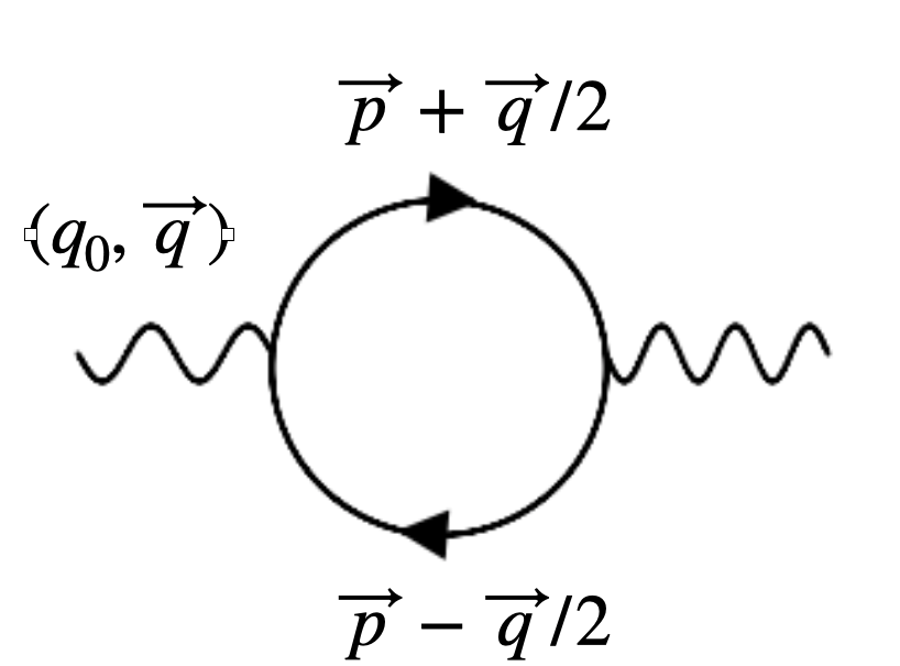
We begin with the (symmetric) energy momentum tensor $\hat{T}^{\mu\nu}$ in terms of the Dirac field:

$\displaystyle\hat{T}^{\mu\nu}=\frac{i}{4}\,\bar{\psi}(\gamma^{\mu}\overleftrightarrow{\partial}^{\nu}+\gamma^{\nu}\overleftrightarrow{\partial}^{\mu})\psi\,.$

(28)

where $\overleftrightarrow{\partial_{\mu}}$ is defined by $A\overleftrightarrow{\partial_{\mu}}B=A\partial_{\mu}B-(\partial_{\mu}A)B$ for arbitrary function $A$ and $B$. Note by definition, $\hat{T}^{\mu\nu}$ is symmetric. Since $\hat{T}^{\mu\nu}=\hat{T}^{\mu\nu}_{1}+\hat{T}^{\mu\nu}_{2}$ contains two terms where $\hat{T}^{\mu\nu}_{1}\equiv(i/4)\,\bar{\psi}\gamma^{j}\overleftrightarrow{\partial}^{0}\psi,\hat{T}^{\mu\nu}_{2}\equiv(i/4)\,\bar{\psi}\gamma^{0}\overleftrightarrow{\partial}^{j}\psi$, we divide correlation function into two parts accordingly:

$\displaystyle G^{\mu,0j}=G^{\mu,0j}_{1}+G^{\mu,0j}_{2}\,,$

(29)

where the $G^{\mu,0j}_{1,2}\sim\langle\left[\hat{{\cal J}}^{\mu}_{5},\hat{T}^{0j}_{1,2}\right]\rangle$. Introducing the Euclidean propagator as function of the Fermionic Matsubara frequency $\nu_{n}=\pi T(2n+1)+\mu$ and momentum $\bm{p}$

	$\displaystyle\,S(i\nu_{n},\bm{p})=\sum_{s=\pm}\,\Lambda_{s}(\bm{p})\,\Delta_{s}(i\nu_{n},\bm{p})\,,$		(30)
	$\displaystyle\,\Lambda_{s}(\bm{p})=s\gamma^{0}\varepsilon_{\bm{p}}-\bm{p}\cdot\bm{\gamma}+m$		(31)
	$\displaystyle\,\Delta_{s}(i\nu_{n},\bm{p})=(\frac{s}{2\varepsilon_{\bm{p}}})\,\frac{1}{i\nu_{n}-s\varepsilon_{\bm{p}}}\,,$		(32)

we can explicitly express correlation function in terms of (Matsubara) frequency and momentum space as

	$\displaystyle\,G^{i,0j}_{1}(i\tilde{\omega}_{n},\bm{q},\bm{p})$	$\displaystyle=\frac{1}{2\beta}\,\sum_{\nu_{n}}\,{\rm Tr}\left[\gamma^{i}\gamma^{5}S\left(i\nu_{n}+i\tilde{\omega}_{n},\bm{p}_{1}\right)\,\gamma^{j}\,(i\nu_{n}+\frac{i\tilde{\omega}_{n}}{2})\,S(i\nu_{n},\bm{p}_{2})\right]$		(33)
	$\displaystyle\,G^{i,0j}_{2}(i\tilde{\omega}_{n},\bm{q},\bm{p})$	$\displaystyle=\frac{1}{2\beta}\,\sum_{\nu_{n}}\,{\rm Tr}\left[\gamma^{i}\gamma^{5}S\left(i\nu_{n}+i\tilde{\omega}_{n},\bm{p}_{1}\right)\,\gamma^{0}\frac{p^{j}_{1}+p^{j}_{2}}{2}\,S(i\nu_{n},\bm{p}_{2})\right]\,$		(34)
	$\displaystyle\,G^{0,0j}(i\tilde{\omega}_{n},\bm{q},\bm{p})$	$\displaystyle=G^{0,0j}_{1}(i\tilde{\omega}_{n},\bm{q},\bm{p})$
		$\displaystyle=\frac{1}{2\beta}\,\sum_{\nu_{n}}\,{\rm Tr}\left[\gamma^{0}\gamma^{5}S\left(i\nu_{n}+i\tilde{\omega}_{n},\bm{p}_{1}\right)\,\gamma^{j}\,(i\nu_{n}+\frac{i\tilde{\omega}_{n}}{2})\,S(i\nu_{n},\bm{p}_{2})\right]\,.$		(35)

Note $\,G^{0,0j}_{2}=0$ due to the trace of the product of the associated gamma matrices vanishes. Here, correlation function depends on Bosonic Matsubara frequency $\tilde{\omega}_{n}=2n\pi T$ and we have defined $\bm{p}_{1}=\bm{p}+\frac{\bm{q}}{2},\bm{p}_{2}=\bm{p}-\frac{\bm{q}}{2}$.

To evaluate correlation functions, we need to take the trace

		$\displaystyle\,X^{ij}_{ss^{\prime}}(\bm{p}_{1},\bm{p}_{2})\equiv{\rm Tr}\left[\gamma^{i}\gamma^{5}\Lambda_{s}(\bm{p}_{1})\,\gamma^{j}\,\Lambda_{s^{\prime}}(\bm{p}_{2})\right]=-4i\epsilon^{ijm}\,\left(s\varepsilon_{1}p_{2}-s^{\prime}\varepsilon_{2}p_{1}\right)_{m}$		(36)
		$\displaystyle\,Y^{i}(\bm{p}_{1},\bm{p}_{2})\equiv{\rm Tr}\left[\gamma^{i}\gamma^{5}\Lambda_{s}(\bm{p}_{1})\,\gamma^{0}\,\Lambda_{s^{\prime}}(\bm{p}_{2})\right]=4i\epsilon^{ijm}\,q_{j}p_{m}\,,$		(37)

and perform the summation over Matsubara frequency:

	$\displaystyle I_{ss^{\prime}}(q_{0},\varepsilon_{1},\varepsilon_{2})$	$\displaystyle=T\sum_{\nu_{n}}\Delta_{s}(i\nu_{n}+i\tilde{\omega}_{n},\bm{p}_{1})\Delta_{s^{\prime}}(i\nu_{n},\bm{p}_{2}))|_{i\omega_{n}\rightarrow q_{0}+i0^{+}}$
		$\displaystyle=\sum_{ss^{\prime}}\left(\frac{-ss^{\prime}}{4\varepsilon_{1}\varepsilon_{2}}\right)\left(\frac{sn_{s}(\varepsilon_{1})-s^{\prime}n_{s^{\prime}}(\varepsilon_{2})}{q_{0}-s\varepsilon_{1}+s^{\prime}\varepsilon_{2}+i0^{+}}\right)$		(38a)
	$\displaystyle J_{ss^{\prime}}(q_{0},\varepsilon_{1},\varepsilon_{2})$	$\displaystyle=T\sum_{\nu_{n}}(i\nu_{n}+\frac{i\tilde{\omega}_{n}}{2})\Delta_{s}(i\nu_{n}+i\tilde{\omega}_{n},\bm{p}_{1})\Delta_{s^{\prime}}(i\nu_{n},\bm{p}_{2})|_{i\omega_{n}\rightarrow q_{0}+i0^{+}}$
		$\displaystyle=(s\varepsilon_{1}-\frac{q_{0}}{2})I_{ss^{\prime}}(q_{0},\varepsilon_{1},\varepsilon_{2})+\frac{s}{4\varepsilon_{1}\varepsilon_{2}}\,n_{s^{\prime}}(\varepsilon_{2}),$		(38b)

To obtain the real time correlation function, we analytically continue the Euclidean correlator by employing the replacement $i\omega_{n}\rightarrow q_{0}+i0^{+}$ in Eq. (38). Note, $0^{+}$ here may be understood as the inverse of relaxation time $\tau^{-1}_{R}$. Here, $\varepsilon_{1,2}=\sqrt{m^{2}+\bm{p}^{2}_{1,2}}$ and $n_{\pm}(\varepsilon)=1/(e^{\beta(\varepsilon\mp\mu)}+1)$ is the Fermi Dirac distribution for particle ($n_{+}$) and antiparticle ($n_{-}$) with chemical potential $\mu$. To obtain the above expression, we use $n_{+}(s\varepsilon)\rightarrow s\,n_{s}(\varepsilon)$ and drop the vacuum contribution “1" in the relation $n_{+}(-\varepsilon)=1-\,n_{-}(\varepsilon)$.

We now express the retarded correlation functions Eq. (33)$\sim$(4) as

		$\displaystyle\,G^{i,0j}_{1}(q_{0},\bm{q},\bm{p})=\frac{1}{2}\sum_{ss^{\prime}}\,X^{ij}_{ss^{\prime}}(\bm{p}_{1},\bm{p}_{2})\,J_{ss^{\prime}}(q_{0},\varepsilon_{1},\varepsilon_{2})\,,$		(39)
		$\displaystyle\,G^{i,0j}_{2}(q_{0},\bm{q},\bm{p})=\frac{1}{2}\,Y^{i}(\bm{p}_{1},\bm{p}_{2})\,p^{j}\,\sum_{ss^{\prime}}\,\,I_{ss^{\prime}}(q_{0},\varepsilon_{1},\varepsilon_{2})\,,$		(40)
		$\displaystyle\,G^{0,0j}_{1}(q_{0},\bm{q},\bm{p})=-\frac{1}{2}\,Y^{j}(\bm{p}_{1},\bm{p}_{2})\,\sum_{ss^{\prime}}J_{ss^{\prime}}(q_{0},\varepsilon_{1},\varepsilon_{2})$		(41)

To proceed, we set up the power counting

$\displaystyle\frac{q_{0}}{\varepsilon_{0}},\frac{q}{\varepsilon_{0}}={\cal O}(\delta_{1})\,$

(42)

where $\delta_{1}$ is a small parameter. Summing up the contribution from $G_{1}$ and $G_{2}$ and expanding the result to the first order of $\delta_{1}$ yield the expression

	$\displaystyle G^{i,0j}_{\pm}(q_{0},\bm{q},\bm{p})$	$\displaystyle=-\frac{i}{2}\epsilon^{ijm}q_{m}\,\left[(\mp\Delta\varepsilon D_{\pm})-b_{\pm}\right]-\frac{i}{2}\epsilon^{ijl}v_{l}\Delta\varepsilon\,q_{0}D_{\pm}$
		$\displaystyle-\frac{i}{2}\epsilon^{iml}q_{m}v_{l}v^{j}\left[(\mp\Delta\varepsilon D_{\pm})+b_{\pm}\right]\,$		(43)
	$\displaystyle G^{0,0j}_{\pm}(q_{0},\bm{q},\bm{p})$	$\displaystyle=\pm\frac{i}{2}\epsilon^{jml}q_{m}v_{l}\,(\mp\Delta\varepsilon D_{\pm}).$		(44)

The first line of Eq. (4) is from $G^{i,0j}_{1,\pm}$ and the second line of Eq. (4) is from $G^{i,0j}_{2,\pm}$. For notational brevity, we have defined

		$\displaystyle\,\bm{v}=\frac{\bm{p}}{\varepsilon_{\bm{p}}}\,,\qquad\Delta\varepsilon=\bm{v}\cdot\bm{q}=-v^{m}q_{m}\,,\qquad D_{\pm}\equiv\frac{a_{\pm}}{q_{0}\mp\Delta\varepsilon+i0^{+}}$		(45)
		$\displaystyle\,a_{\pm}=-\frac{\partial n_{\pm}(\varepsilon_{\bm{p}})}{\partial\varepsilon_{\bm{p}}}=\beta\,n_{\pm}(\varepsilon_{\bm{p}})\left(1-n_{\pm}(\varepsilon_{\bm{p}})\right)\,,\qquad b_{\pm}\equiv\frac{n_{\pm}(\varepsilon_{\bm{p}})}{\varepsilon_{\bm{p}}}\,.$		(46)

As we discussed earlier, we need to decompose $G^{i,0j}$ (and similarly for other correlation functions) into two parts, $G^{i,0j}_{\pm}$ (see Eq. (17)), so that the induced axial current distribution for fermions and anti-fermions are given by Eq. (15). Observing that ${\cal A}_{+}$ (${\cal A}_{-}$) should only depend on $a_{+},b_{+}$ ($a_{-},b_{-}$), we simply group terms associated with $D_{+}$ and $b_{+}$ are grouped to $G_{R,+}$ and perform the similar procedure for $G_{-}$.

We are now ready to take the slow/fast limits as defined in the previous section. Noting

		$\displaystyle\,\lim_{\textbf{s}}(\mp\Delta\varepsilon D_{\pm})=a_{\pm}\,,\qquad\lim_{\textbf{f}}(q_{0}D_{\pm})=0\,,$		(47)
		$\displaystyle\,\lim_{\textbf{s}}(\mp\Delta\varepsilon D_{\pm})=0\,,\qquad\lim_{\textbf{f}}(q_{0}D_{\pm})=a_{\pm}\,,$		(48)

it immediately follows from Eq. (4) and Eq. (44) that:

	$\displaystyle\frac{i\partial}{\partial q_{m}}$	$\displaystyle\lim_{\textbf{s}}G^{i,0j}_{\pm}=\frac{1}{2}\,\epsilon^{ijm}(a_{\pm}-b_{\pm})+\frac{1}{2}\epsilon^{iml}v_{l}v^{j}(a_{\pm}+b_{\pm})$		(49)
		$\displaystyle\frac{i\partial}{\partial q_{m}}\lim_{\textbf{f}}G^{i,0j}_{\pm}=-\frac{1}{2}\,\epsilon^{ijm}b_{\pm}-\frac{1}{2}\,\epsilon^{ijl}v_{l}\,v^{m}a_{\pm}+\frac{1}{2}\epsilon^{iml}v_{l}v^{j}b_{\pm}$		(50)

Finally, we have:

$\displaystyle\,\kappa^{ijm}_{\pm}=\lim_{\textbf{s-f}}\frac{i\partial}{\partial q_{m}}G^{i,0j}_{\pm}=\frac{1}{2}a_{\pm}(-\epsilon^{imj}+\epsilon^{iml}v_{l}v^{j}+\,\epsilon^{ijl}v_{l}\,v^{m})$

(51)

Similarly, we have

$\displaystyle\lim_{\textbf{s-f}}\frac{i\partial}{\partial q_{m}}G^{0,0j}_{\pm}=\mp\frac{1}{2}\epsilon^{jml}v_{l}\,a_{\pm}\,.$

(52)

With Eqs. (51), (52) at hand, we can extract the transport functions, as we shall do in the next section.

References

- (1) Z.-T. Liang and X.-N. Wang, Globally polarized quark-gluon plasma in non-central A+A collisions, Phys. Rev. Lett. 94 (2005) 102301.
- (2) F. Becattini, V. Chandra, L. Del Zanna and E. Grossi, Relativistic distribution function for particles with spin at local thermodynamical equilibrium, Annals Phys. 338 (2013) 32.
- (3) F. Becattini, Polarization in relativistic fluids: a quantum field theoretical derivation, 4, 2020, 2004.04050.
- (4) W. Florkowski, B. Friman, A. Jaiswal and E. Speranza, Relativistic fluid dynamics with spin, Phys. Rev. C 97 (2018) 041901 [1705.00587].
- (5) K. Hattori, M. Hongo, X.-G. Huang, M. Matsuo and H. Taya, Fate of spin polarization in a relativistic fluid: An entropy-current analysis, Phys. Lett. B 795 (2019) 100 [1901.06615].
- (6) S. Y. F. Liu, Y. Sun and C. M. Ko, Spin Polarizations in a Covariant Angular-Momentum-Conserved Chiral Transport Model, Phys. Rev. Lett. 125 (2020) 062301 [1910.06774].
- (7) K. Fukushima and S. Pu, Spin Hydrodynamics and Symmetric Energy-Momentum Tensors – A current induced by the spin vorticity –, 2010.01608.
- (8) S. Shi, C. Gale and S. Jeon, Relativistic Viscous Spin Hydrodynamics from Chiral Kinetic Theory, 2008.08618.
- (9) S. Li, M. A. Stephanov and H.-U. Yee, Non-dissipative second-order transport, spin, and pseudo-gauge transformations in hydrodynamics, 2011.12318.
- (10) R. Singh, G. Sophys and R. Ryblewski, Spin polarization dynamics in the Gubser-expanding background, 2011.14907.
- (11) STAR collaboration, L. Adamczyk et al., Global hyperon polarization in nuclear collisions: evidence for the most vortical fluid, Nature 548 (2017) 62.
- (12) STAR collaboration, J. Adam et al., Global polarization of hyperons in Au+Au collisions at = 200 GeV, Phys. Rev. C 98 (2018) 014910 [1805.04400].
- (13) STAR collaboration, T. Niida, Global and local polarization of hyperons in Au+Au collisions at 200 GeV from STAR, Nucl. Phys. A 982 (2019) 511.
- (14) STAR collaboration, J. Adam et al., Polarization of () hyperons along the beam direction in Au+Au collisions at = 200 GeV, Phys. Rev. Lett. 123 (2019) 132301 [1905.11917].
- (15) F. Becattini and I. Karpenko, Collective Longitudinal Polarization in Relativistic Heavy-Ion Collisions at Very High Energy, Phys. Rev. Lett. 120 (2018) 012302.
- (16) X.-L. Xia, H. Li, Z.-B. Tang and Q. Wang, Probing vorticity structure in heavy-ion collisions by local polarization, Phys. Rev. C 98 (2018) 024905 [1803.00867].
- (17) J.-Y. Chen, D. T. Son, M. A. Stephanov, H.-U. Yee and Y. Yin, Lorentz Invariance in Chiral Kinetic Theory, Phys. Rev. Lett. 113 (2014) 182302.
- (18) J.-Y. Chen, D. T. Son and M. A. Stephanov, Collisions in Chiral Kinetic Theory, Phys. Rev. Lett. 115 (2015) 021601.
- (19) K. Hattori, Y. Hidaka and D.-L. Yang, Axial Kinetic Theory and Spin Transport for Fermions with Arbitrary Mass, Phys. Rev. D 100 (2019) 096011 [1903.01653].
- (20) S. A. Crooker and D. L. Smith, Imaging spin flows in semiconductors subject to electric, magnetic, and strain fields, Physical Review Letters 94 (2005) .
- (21) A. G. Mal’Shukov, C. S. Tang, C. S. Chu and K. A. Chao, Strain-Induced Coupling of Spin Current to Nanomechanical Oscillations, Phys.Rev.Lett 95 (2005) 107203 [cond-mat/0504773].
- (22) D. E. Kharzeev, M. A. Stephanov and H.-U. Yee, Anatomy of chiral magnetic effect in and out of equilibrium, Phys. Rev. D 95 (2017) 051901 [1612.01674].
- (23) S. Y. F. Liu and Y. Yin, Spin Hall effect in heavy ion collisions, 2006.12421.
- (24) J. M. Luttinger, Theory of thermal transport coefficients, Phys. Rev. 135 (1964) A1505.
- (25) Y.-C. Liu, K. Mameda and X.-G. Huang, Covariant Spin Kinetic Theory I: Collisionless Limit, Chin. Phys. C 44 (2020) 094101 [2002.03753].
- (26) T. Hayata, Y. Hidaka and K. Mameda, Second order chiral kinetic theory under gravity and antiparallel charge-energy flow, 2012.12494.
- (27) K. Landsteiner, E. Megias, L. Melgar and F. Pena-Benitez, Holographic Gravitational Anomaly and Chiral Vortical Effect, JHEP 09 (2011) 121 [1107.0368].
- (28) S. Lin and L. Yang, Mass correction to chiral vortical effect and chiral separation effect, Phys. Rev. D98 (2018) 114022 [1810.02979].
- (29) R.-h. Fang, L.-g. Pang, Q. Wang and X.-n. Wang, Polarization of massive fermions in a vortical fluid, Phys. Rev. C94 (2016) 024904 [1604.04036].
- (30) H.-Z. Wu, L.-G. Pang, X.-G. Huang and Q. Wang, Local spin polarization in high energy heavy ion collisions, Phys. Rev. Research. 1 (2019) 033058 [1906.09385].
- (31) W. Florkowski, A. Kumar, R. Ryblewski and A. Mazeliauskas, Longitudinal spin polarization in a thermal model, Phys. Rev. C 100 (2019) 054907 [1904.00002].
- (32) D. T. Son and N. Yamamoto, Berry Curvature, Triangle Anomalies, and the Chiral Magnetic Effect in Fermi Liquids, Phys. Rev. Lett. 109 (2012) 181602 [1203.2697].
- (33) M. Stephanov and Y. Yin, Chiral Kinetic Theory, Phys. Rev. Lett. 109 (2012) 162001 [1207.0747].
- (34) N. Mueller and R. Venugopalan, Worldline construction of a covariant chiral kinetic theory, Phys. Rev. D 96 (2017) 016023 [1702.01233].
- (35) N. Mueller and R. Venugopalan, Constructing phase space distributions with internal symmetries, Phys. Rev. D 99 (2019) 056003 [1901.10492].
- (36) N. Weickgenannt, X.-L. Sheng, E. Speranza, Q. Wang and D. H. Rischke, Kinetic theory for massive spin-1/2 particles from the Wigner-function formalism, Phys. Rev. D 100 (2019) 056018 [1902.06513].
- (37) N. Weickgenannt, E. Speranza, X.-l. Sheng, Q. Wang and D. H. Rischke, Generating spin polarization from vorticity through nonlocal collisions, 2005.01506.
- (38) B. Fu, S. Y. F. Liu, L. Pang, H. Song and Y. Yin, Shear-induced spin polarization in heavy-ion collisions, 2103.10403.
- (39) D. Hou and S. Lin, Polarization Rotation of Chiral Fermions in Vortical Fluid, 2008.03862.