跳到论文正文
W Papers独立论文阅读器 arXiv:2103.09121 论文正文 计算阅读时间 · 0%
引用这篇论文根据当前论文元数据生成,正式投稿前建议核对。


License: arXiv.org perpetual non-exclusive license
arXiv:2103.09121v1 [q-fin.RM] 16 Mar 2021

Robust equilibrium strategies in a defined benefit pension plan game

Guohui Guana,∗, Jiaqi Hub,†, Zongxia Liangb,‡ aSchool of Statistics, Renmin University of China, Beijing 100872, China bDepartment of Mathematical Sciences, Tsinghua University, Beijing 100084, China Note: $ˆ*$ e-mail: guangh@ruc.edu.cn
$ˆ†$ Corresponding author, e-mail: hujq20@mails.tsinghua.edu.cn
$‡$ e-mail: liangzongxia@mail.tsinghua.edu.cn
Abstract.

This paper investigates the robust non-zero-sum games in an aggregated overfunded defined benefit (abbr. DB) pension plan. The sponsoring firm is concerned with the investment performance of the fund surplus while the participants act as a union to claim a share of the fund surplus. The financial market consists of one risk-free asset and nn risky assets. The firm and the union both are ambiguous about the financial market and care about the robust strategies under the worst case scenario. The union’s objective is to maximize the expected discounted utility of the additional benefits, the firm’s two different objectives are to maximizing the expected discounted utility of the fund surplus and the probability of the fund surplus reaching an upper level before hitting a lower level in the worst case scenario. We formulate the related two robust non-zero-sum games for the firm and the union. Explicit forms and optimality of the solutions are shown by stochastic dynamic programming method. In the end of this paper, numerical results are illustrated to depict the economic behaviours of the robust equilibrium strategies in these two different games.

JEL classification: C61,G11, G22, D53.

2020 Mathematics Subject Classification: 91G05, 91B50, 91A11, 91A15, 91G10.

Submission Classification: IE11, IE13, IM50, IB81.

Keywords: Overfunded DB pension plan; Robust control; Stochastic differential game; Nash equilibrium; Stochastic dynamic programming.

1. Introduction

With the aging of population worldwide, retirement plan plays an important role in ensuring the quality of life of the elders. Although there is a recent shift from the DB pension plan to the defined contribution (abbr. DC) pension plan, DB pension plan is still very important in retirement welfare policy. The benefits of the participants in DB pension plan are fixed in advance and the contribution rates are calculated and adjusted to keep actuarial balance. In a DB pension plan, benefits are distributed at retirement as an annuity or one lump-sum payment, and constitute the main liability of the firm. Besides, the contributions from the participants constitute the assets of the firm. In order to hedge financial risk, the firm allocates the wealth of the fund in the financial market.

When the asset of the firm is lower than its liability, the pension fund is underfunded. A study by investment bank Credit Suisse First Boston (CSFB) finds that at the end of 2001, there are more companies in the S&P 500 with underfunded DB pension plans than at any time during the previous 10 years. When the pension fund is underfunded, the firm is faced with insolvency risk and aims to minimize the gap between the liability and asset. Many previous studies in DB pension fund focus on the underfunded case, see e.g., Haberman and Sung, 1994, Haberman et al., 2000, Josa-Fombellida and Rincón-Zapatero, 2004, etc. Most of recent work consider more financial risks for the underfunded DB pension plan and can help manage the fund better, see interest risk in Huang and Cairns, 2006, Hainaut et al., 2011, jump risk in Josa-Fombellida and Rincón-Zapatero, 2012, volatility risk in Josa-Fombellida et al., 2018, etc.

Although most of the pension plans are underfunded, overfunding may also happen because of the outstanding performance of the investment, particularly in the bull market, or the premature death of a high paid employee. Table II(c) in Severinson, 2008 illustrates that a small proportion of companies are overfunded. Howard, 2019 show that within the S&P 500, 46 companies had overfunded pensions in 2018 (up from 43 in 2017). Overfunded DB pension plan has its own issues about how to manage the excess assets. Reversion when liquidated, increasing plan benefits, allowing additional accruals, adding plan participants may be possible tools to manage the excess assets. However, an excise tax 50% is ultimately imposed on plan reversion. Haw et al., 1988 show that firms terminating overfunded pension plans tend to have tax loss from termination. Harper and Treanor, 2014 indicate that the firms have a desire to modify the implicit contract instead of terminating the plan. As such, distributing benefits to plan participants is a better tool in an overfunded pension fund. In Josa-Fombellida and Rincón-Zapatero, 2019, the authors assume that in the overfunded DB pension plan, the participants claim a share of the fund surplus as additional benefits. On the one hand, increasing plan benefits can avoid the tax from termination. On the other hand, the additional benefits can attract more potential participants.

Josa-Fombellida and Rincón-Zapatero, 2019 present games for the firm and the union. The firm cares about the wealth of the fund surplus and has two goals while the participants aim to acquire more additional benefits from the fund. The explicit solutions of the equilibrium strategies are derived in Josa-Fombellida and Rincón-Zapatero, 2019, their results show that the strategies rely heavily on the parameters of the financial market. The equilibrium game in Guan and Liang, 2016 for the DC pension fund also shows the great impacts of parameters on the strategies. However, as the limited information of the financial market, the investors can not observe the financial market accurately and are in fact ambiguity averse when making decisions, see Hansen and Sargent, 2001, Binmore et al., 2012, Guan et al., 2018, Guan and Liang, 2019, etc. In the management of DC pension fund, Sun et al., 2018, Wang and Li, 2018 and Wang et al., 2019b implicate that when ignoring ambiguity, the manager is faced with large utility losses. As such, model uncertainty should be considered in risk management.

In this paper, we study the robust equilibrium games between the firm and participants. The goals ignoring ambiguity are the same as in Josa-Fombellida and Rincón-Zapatero, 2019 and then modified to introduce ambiguity aversion for the players. The firm and participants seek the robust equilibrium strategies under worst case scenario. In fact, recently, there are some literature about the robust equilibrium games, see Pun and Wong, 2016, Wang et al., 2019a, Wang et al., 2021, etc. These mentioned work concerning robust equilibrium game mainly consider two separate agents and the agents care about the relative performance over the other. Besides, both the agents have the same instruments to manage the wealth. However, in our work, the decisions made by the firm and participants affect the same wealth process. The firm and participants have different tools: the firm chooses the investment in the financial market, the participants decide the amount of additional benefits. Moreover, the previous mentioned work suppose that the agents will never go bankruptcy and are concerned with the wealth of the agents at a fixed time. In this paper, we consider two different goals for the firm: maximizing the expected discounted utility of the fund surplus and the probability of the fund surplus reaching an upper level before hitting a lower level. On the one hand, our goals are more abundant and provide guidance for different kinds of agents. On the other hand, concerning the robust optimization problem at a fixed time, the procedure in Mataramvura and Øksendal, 2008 can be well applied to show the optimality of the robust equilibrium strategies. The goals in our paper are different from the optimization rule in Mataramvura and Øksendal, 2008 and detailed verification theorem is required.

Using stochastic dynamic programming method, we present and derive the explicit forms of the robust equilibrium strategies of the firm and participants. Numerical results are also shown for the two players. We see that the firm and participants act very differently in the bull and bear markets. In addition, ambiguity aversion influences both the firm and the participants’ decisions. We have the main contributions in this paper: First, we present the robust equilibrium games of the firm and participants under two different objectives. The robust control of maximizing the probability of reaching an upper level is relatively different from previous work. We see that in order to obtain the explicit solution, the penalty term for this kind of objective is also relatively different. Second, using stochastic dynamic programming method, we present the HJBI system of the robust games and derive the explicit forms of the robust investment strategy and benefit. For the first game, we also present detailed analysis over the robust equilibrium strategies and show the Pareto optimality under some case. Third, most previous work study the robust control about the terminal wealth, which is also different from ours. Inspired by Mataramvura and Øksendal, 2008, we define the admissible sets strictly and propose another condition to replace the uniformly integrability condition to show the verification theorem. Last, numerical analyses are illustrated to depict the players’ economic behaviours. Ambiguity aversion will always prompt the participants to ask for fewer benefits whether the economy is booming or sluggish, but this effect is minimal when the economy is in recession. For the first game, the ambiguity aversions of the two parties have different effects on the participants’ strategy.

The reminder of this paper is organized as follows. Section 2 presents the formulation of the overfunded DB pension plan under model uncertainty. In Section 3, we introduce two different robust equilibrium games for the firm and the union. Section 4 shows the admissible sets of the robust equilibrium problems and derives the explicit forms of equilibrium strategies, worst case measures and value functions. Optimality of the strategies is verified strictly. The numerical results about the robust equilibrium strategies are illustrated in Section 5. Section 6 concludes this paper. Most of the proofs are in Appendix.

2. DB pension fund game

In this section, we present the financial model of the overfunded DB pension fund. The sponsoring firm invests the fund surplus in the financial market and is concerned with the investment performance of the fund. To be more attractive, the overfunded pension fund provides excess benefits to the participants as a union. We consider a financial market similar with Josa-Fombellida and Rincón-Zapatero, 2019 consisting of one risk-free asset and nn risky assets for simplicity.

Consider a filtered complete probability space (Ω,ℱ,{ℱt}t≥0,ℙ)\left(\Omega,\mathcal{F},\left\{\mathcal{F}_{t}\right\}_{t\geq 0},\mathbb{P}\right). ℱt\mathcal{F}_{t} represents the information of the financial market up to time tt. Different from Josa-Fombellida and Rincón-Zapatero, 2019, we suppose that the firm and the union are both uncertain about the financial market and ℙ\mathbb{P} is the reference probability measure of the market. In order to apply the Girsanov’s Theorem in infinite time horizon (see Corollary 5.2 and Proposition 5.12 of Chapter III in Karatzas and Shreve, 1991), the probability space is specified: Ω=C[0,∞)n\Omega=C\left[0,\infty\right)^{n}, W={W⁡(t):t≥0}W=\{W\left(t\right):t\geq 0\} is the coordinate mapping process on Ω\Omega, ℙ\mathbb{P} is the Wiener measure on (Ω,ℱ)\left(\Omega,\mathcal{F}\right) and {ℱt}t≥0\left\{\mathcal{F}_{t}\right\}_{t\geq 0} is the filtration generated by WW. Obviously, W=(W1,W2,⋯,Wn)TW=(W_{1},W_{2},\cdots,W_{n})^{T} is an nn-dimensional standard Brownian motion on the space (Ω,ℱ,{ℱt}t≥0,ℙ)\left(\Omega,\mathcal{F},\left\{\mathcal{F}_{t}\right\}_{t\geq 0},\mathbb{P}\right). We do not consider transaction costs in this paper. All the processes introduced are supposed to be well defined and adapted to {ℱt}t≥0\left\{\mathcal{F}_{t}\right\}_{t\geq 0}.

2.1. Financial model

The firm sponsoring the fund invests in the financial market and expects that the fund surplus increases. For simplicity, we only consider equity risk and suppose that there are one risk-free asset S0S^{0} and nn risky assets S1,S2⋯,SnS^{1},S^{2}\cdots,S^{n} in the financial market. The dynamics of these n+1n+1 assets are

(2.1) d​S0​(t)\displaystyle\mathrm{d}S^{0}\left(t\right)\! =\displaystyle= r​S0​(t)​d​t,S0​(0)=1,\displaystyle rS^{0}\left(t\right)\mathrm{d}t,\!\quad S^{0}\left(0\right)=1,
(2.2) d​Si​(t)\displaystyle\mathrm{d}S^{i}\left(t\right)\! =\displaystyle= Si​(t)​(bi​d​t+∑i=1nσi​j​d​Wj​(t)),Si​(0)=si,i=1,⋯,n,\displaystyle S^{i}\!\left(t\right)\!\left(b_{i}\mathrm{d}t+\sum_{i=1}^{n}\!\sigma_{ij}\mathrm{d}W_{j}\left(t\right)\right),S^{i}\left(0\right)=s_{i},\!i=1,\cdots,n,\!

where r>0r>0 is the risk-free interest rate, bi>rb_{i}>r is the mean rate of return of the risky asset SiS^{i}, and σi​j>0\sigma_{ij}>0 represents the volatility coefficient. Denote σ=(σi​j)n×n\sigma=\left(\sigma_{ij}\right)_{n\times n} as the volatility matrix of the risky assets. Let b=(b1,b2,⋯,bn)Tb=(b_{1},b_{2},\cdots,b_{n})^{T} and 1→=(1,⋯,1)T∈𝐑n\vec{1}=(1,\cdots,1)^{T}\in\mathbf{R}^{n}. The Sharpe ratio vector is θ=σ−1​(b−r​1→)\theta=\sigma^{-1}(b-r\vec{1}). We assume that the financial market is complete, i.e., the matrix Σ≜σ​σT\Sigma\triangleq\sigma\sigma^{T} is positive definite.

In the financial market, we suppose that the pension fund is overfunded. Different from the management of an underfunded pension fund, the firm is endowed with a positive surplus at initial time and invests in the financial market. In order to be more attractive, the participants in the pension fund also expect to enjoy the benefits of this positive surplus process. As in Josa-Fombellida and Rincón-Zapatero, 2019, the union of the participants claims part of the fund surplus continuously. We assume that the number of the participants is stable, which means that we do not consider longevity risk in our work.

Let X={X⁡(t):t≥s}X=\{X(t):t\geq s\} be the surplus process of the DB pension fund with positive value X⁡(s)=xX\left(s\right)=x at initial time s≥0s\geq 0. The firm invests an amount of πi={πi​(t):t≥s}\pi_{i}=\{\pi_{i}(t):t\geq s\} in SiS^{i}. The rest part π0=X−∑i=1nπi\pi_{0}=X-\sum_{i=1}^{n}\pi_{i} is allocated in the risk-free asset S0S^{0}. Denote π=(π1,⋯,πn)T\pi=\left(\pi_{1},\cdots,\pi_{n}\right)^{T} as the investment strategy of the firm. The union claims benefit P={P⁡(t):t≥s}P=\{P(t):t\geq s\} from the pension fund continuously. The firm is concerned with the surplus process XX while the union cares about the benefit PP. Their decisions π\pi and PP both affect XX. By adopting strategy (π,P)(\pi,P), the surplus process XX is given by

d​X​(t)=∑i=0nπi​(t)​d​Si​(t)Si​(t)−P⁡(t)​d​t,X⁡(s)=x.\mathrm{d}X(t)=\sum_{i=0}^{n}\pi_{i}(t)\frac{\mathrm{d}S^{i}(t)}{S^{i}(t)}-P(t)\mathrm{d}t,\ \ X(s)=x.

As we consider a stable pension system, the surplus process totally depends on the investment performance of the firm, the benefits of the union and the initial endowment. There is a trade-off here for the benefits: on the one hand, larger PP means more current benefit, on the other hand, the fund surplus becomes small and the fund may become underfunded when PP is large. Substituting Eqs. (2.1) and (2.2) into the last equation, the surplus process XX follows

(2.3) {d​X​(t)=[r​X​(t)+πT​(t)​(b−r​1→)−P⁡(t)]​d​t+πT​(t)​σ​d​W​(t),X⁡(s)=x.\begin{cases}\mathrm{d}X\left(t\right)=\left[rX\left(t\right)+\pi^{T}\left(t\right)\left(b-r\vec{1}\right)-P\left(t\right)\right]\mathrm{d}t+\pi^{T}\left(t\right)\sigma\,\mathrm{d}W\left(t\right),\\ X\left(s\right)=x.\end{cases}

Both the firm and the union can observe the fund surplus and know exactly the current value of the fund when making decisions. As such, the trading strategy π\pi and the benefit PP depend on the surplus process XX, i.e., π⁡(t)\pi\left(t\right) and P⁡(t)P\left(t\right) have the form π⁡(t)=π⁡(t,X⁡(t))\pi\left(t\right)=\pi\left(t,X\left(t\right)\right), P⁡(t)=P⁡(t,X⁡(t))P\left(t\right)=P\left(t,X\left(t\right)\right) at time tt. In fact, as the system is Markovian and stationary, π\pi and PP have the form π=π⁡(x)\pi=\pi(x), P=P⁡(x)P=P(x), which is shown in Josa-Fombellida and Rincón-Zapatero, 2019 and means that the strategies only depend on the current wealth of the fund surplus. In our paper with ambiguity aversion, this dependence is also required, and we will see that the robust equilibrium strategies are of these forms.

2.2. Ambiguity aversion

The financial model we consider is similar with the model presented in Josa-Fombellida and Rincón-Zapatero, 2019. However, in their work, the firm and the union can observe the financial model accurately, i.e., the probability measure ℙ\mathbb{P} is the real probability measure of the financial market. However, as shown in Blanchard et al., 1993, the first moments of the assets are hard to be estimated accurately. When the investor makes decisions ignoring model uncertainty, he will be faced with large utility loss, see Yi et al., 2013, Huang et al., 2017, etc. Ambiguity aversion is a way to characterize the decision maker’s attitude towards model uncertainty. Particularly in the long term management of a DB pension fund, it is necessary to consider model uncertainty and characterize the firm (union)’s ambiguity aversion. In what follows, similar with Maenhout, 2004 and Maenhout, 2006, we characterize model uncertainty by a set of equivalent probability measures.

We suppose that the firm and the union both are ambiguity averse, i.e., both of them are concerned about the accuracy of the reference model. We define a set of equivalent probability measures to ℙ\mathbb{P} by

𝒬:={ℚ|ℚ∼ℙ}.\mathcal{Q}:=\{\mathbb{Q}|\mathbb{Q}\sim\mathbb{P}\}.

The firm and the union are not fully confident about the reference probability measure ℙ\mathbb{P} and consider the set 𝒬\mathcal{Q} when making decisions. Each probability measure ℚ∈𝒬\mathbb{Q}\in\mathcal{Q} represents a possible actual financial model.

For s≥0s\geq 0 and x>0x>0, let 𝐄s,x​Y\mathbf{E}_{s,x}Y denote the expectation of random variable YY under the condition X⁡(s)=xX\left(s\right)=x. Especially, when s=0s=0, it is written as 𝐄x​Y\mathbf{E}_{x}Y for short. In order to show 𝒬\mathcal{Q} more clearly, we consider a set of nn-dimensional-valued processes ℋ≜{h={h(t):t≥s}}\mathcal{H}\triangleq\{h=\{h(t):t\geq s\}\} satisfying:

  1. (1)

    hh is progressively measurable w.r.t. the filtration {ℱt}t≥s\{\mathcal{F}_{t}\}_{t\geq s}.

  2. (2)

    For x>0x>0 with initial condition X⁡(s)=xX(s)=x, the following Novikov’s condition holds:

    𝐄s,x​[exp⁡{∫sThT​(t)​h​(t)2​𝑑t}]<∞,∀T≥s.\mathbf{E}_{s,x}\left[\exp\left\{\int_{s}^{T}\frac{h^{T}\left(t\right)h\left(t\right)}{2}\mathrm{d}t\right\}\right]<\infty,\quad\forall T\geq s.

Based on Corollary 5.2 and Proposition 5.12 in Chapter III of Karatzas and Shreve, 1991, for h∈ℋh\in\mathcal{H}, there is a unique equivalent measure ℚh\mathbb{Q}^{h} of ℙ\mathbb{P} on the space (Ω,ℱ,{ℱt}t≥s)\left(\Omega,\mathcal{F},\left\{\mathcal{F}_{t}\right\}_{t\geq s}\right) with

d​ℚhd​ℙ|ℱt=Θh​(t),\frac{\mathrm{d}\mathbb{Q}^{h}}{\mathrm{d}\mathbb{P}}|_{\mathcal{F}_{t}}=\Theta^{h}(t),

where {Θh​(t):t≥s}\{\Theta^{h}(t):t\geq s\} is a ℙ−\mathbb{P}-martingale defined by

Θh​(t)=exp⁡{∫sth​(s)T​dW​(s)−12​∫sth​(s)T​h​(s)​ds}.\begin{split}\Theta^{h}(t)=\exp\left\{\int_{s}^{t}h(s)^{T}\mathrm{d}W(s)-\frac{1}{2}\int_{s}^{t}h(s)^{T}h(s)\mathrm{d}s\right\}.\end{split}

Based on Girsanov’s Theorem, the following process is an nn-dimensional standard Brownian motion under ℚh\mathbb{Q}^{h}

d​Wh​(t)=d​W​(t)+h⁡(t)​d​t.\mathrm{d}W^{h}\left(t\right)=\mathrm{d}W\left(t\right)+h\left(t\right)\mathrm{d}t.
Remark 1.

In the following, the expectation under the probability measure ℚh\mathbb{Q}^{h} is denoted by 𝐄s,xh​[⋅]\mathbf{E}^{h}_{s,x}[\cdot] (or 𝐄xh​[⋅]\mathbf{E}^{h}_{x}[\cdot]).

Under the ℚh\mathbb{Q}^{h}, the fund surplus XX follows

(2.4) {d​X​(t)=[r​X​(t)+πT​(t)​(b−r​1→)−P⁡(t)−πT​(t)​σ​h​(t)]​d​t+πT​(t)​σ​d​Wh​(t),X⁡(s)=x.\displaystyle\begin{cases}\mathrm{d}X\left(t\right)=&\left[rX\left(t\right)+\pi^{T}\left(t\right)\left(b-r\vec{1}\right)-P\left(t\right)-\pi^{T}\left(t\right)\sigma h\left(t\right)\right]\mathrm{d}t\\ &+\pi^{T}\left(t\right)\sigma\,\mathrm{d}W^{h}\left(t\right),\\ X\left(s\right)=&x.\end{cases}

Different from the financial model in Josa-Fombellida and Rincón-Zapatero, 2019, the wealth process includes an additional process hh to describe the model uncertainty. Meanwhile, in our framework, we are mainly concerned with model uncertainty of the first moments of the yields of the stock and hh only affects the drift terms in the wealth process. There are two players in our financial model and they have different ambiguity aversions. We denote processes hFh_{F} and hUh_{U} as the measure transformation processes of the firm and the union, respectively.

3. Robust equilibrium games

In this section, we present two different robust games for the firm and the union. The strategies taken by the firm and the union affect the fund surplus. The goals of the firm and the union are relatively opposite. The union expects to claim more benefits from the fund while the firm tries to increase the wealth of the fund. As such, they form a non-zero-sum game when making decisions and we are concerned with their Nash equilibrium strategies. Generally for an insurance company, there are two optimization rules: maximizing the expected wealth and minimizing the probability of ruin, see Browne, 1995. In Josa-Fombellida and Rincón-Zapatero, 2019, they show two similar different objectives for the firm. The union often does not care about the stability of the fund and aims to maximize the total expected future benefits from the fund. In the following, we present two different objectives for the firm and one objective for the union.

3.1. The first game: Maximizing the expected wealth

In some cases, the firm is concerned with the expected utility of the fund surplus. When ignoring ambiguity, given PP, the firm chooses π\pi to maximize the payoff

(3.1) jF​(s,x,π,P)=𝐄s,x​[∫s∞e−β​t​v​(X⁡(t))​𝑑t],j_{F}\left(s,x;\pi,P\right)=\mathbf{E}_{s,x}\left[\int_{s}^{\infty}e^{-\beta t}v\left(X\left(t\right)\right)\mathrm{d}t\right],

where v⁡(⋅)v\left(\cdot\right) is a utility function and β>0\beta>0 is the time preference of the firm. Besides, given π\pi, the union seeks PP to maximize the payoff

(3.2) jU​(s,x,π,P)=𝐄s,x​[∫s∞e−α​t​u​(P⁡(t))​𝑑t],j_{U}\left(s,x;\pi,P\right)=\mathbf{E}_{s,x}\left[\int_{s}^{\infty}e^{-\alpha t}u\left(P\left(t\right)\right)\mathrm{d}t\right],

where u⁡(⋅)u\left(\cdot\right) is a utility function and α>0\alpha>0 is the time preference of the union.

The two objectives (3.1) and (3.2) have been shown in Josa-Fombellida and Rincón-Zapatero, 2019. They also obtain the explicit forms of equilibrium strategies (π∗,P∗)(\pi^{*},P^{*}) under these two objectives. In our work, we are interested in the effect of model uncertainty on the firm and the union’s behaviours. Next, we present the objectives under model uncertainty. In spite that the firm and the union are ambiguity averse, the original probability measure ℙ\mathbb{P} has reference value and the new measure ℚh\mathbb{Q}^{h} can not deviate too far from the original measure. As in Maenhout, 2004, Maenhout, 2006, Gu et al., 2020, etc., we add a penalty term after the expected discounted utility jU​(s,x,π,P)j_{U}\left(s,x;\pi,P\right) (jF​(s,x,π,P)j_{F}\left(s,x;\pi,P\right)) as the payoff function under ambiguity, as such, the payoff of the union under ambiguity is

(3.3) JU​(s,x,π,P,hU):=𝐄s,xhU​[∫s∞e−α​t​u​(P⁡(t))​𝑑t+∫s∞e−α​t​12​hUT​(t)​hU​(t)φU​(t,X​(t))​𝑑t].\displaystyle J_{U}\left(s,x,\pi,P,h_{U}\right):=\mathbf{E}_{s,x}^{h_{U}}\left[\int_{s}^{\infty}e^{-\alpha t}u\left(P\left(t\right)\right)\mathrm{d}t\!+\!\int_{s}^{\infty}e^{-\alpha t}\frac{\frac{1}{2}h_{U}^{T}\left(t\right)h_{U}\left(t\right)}{\varphi_{U}\left(t,X\left(t\right)\right)}\mathrm{d}t\right].

The increasing rate of the relative entropy from time tt to time t+d​tt+\mathrm{d}t equals hT​(t)​h​(t)h^{T}(t)h(t), which has been shown in Li et al., 2018. φU​(t,X​(t))\varphi_{U}\left(t,X\left(t\right)\right) represents the degree of ambiguity aversion. When φU​(t,X​(t))\varphi_{U}\left(t,X\left(t\right)\right) increases, the union has less confidence about the reference model.

In this paper, u⁡(P)u\left(P\right) is the CRRA utility function, i.e.,

u⁡(P)=P1−γ1−γ,γ>0,γ≠1,u\left(P\right)=\frac{P^{1-\gamma}}{1-\gamma},\quad\gamma>0,\quad\gamma\neq 1,

where γ\gamma represents the risk aversion of the union over financial risk. Besides, we suppose

φU​(t,x)=λ(1−γ)​JU​(t,x,π,P,hU),\varphi_{U}\left(t,x\right)=\frac{\lambda}{\left(1-\gamma\right)J_{U}\left(t,x,\pi,P,h_{U}\right)},

where λ>0\lambda>0 is the ambiguity aversion parameter of the union. φU​(t,x)\varphi_{U}\left(t,x\right) is positive and is inversely proportional to the payoff function. When λ\lambda increases, the union has less faith in the reference model.

Remark 2.

It is worth noting here that XX actually depends on the strategy variable (π,P)(\pi,P), and φU​(t,x)\varphi_{U}\left(t,x\right) also depends on the strategy variable (π,P)(\pi,P) and the process hUh_{U}. However, for simplicity, (π,P)(\pi,P) is omitted and not shown in XX, so as the following φ^U​(x),φF​(t,x)\hat{\varphi}_{U}\left(x\right),\varphi_{F}\left(t,x\right) and φ^F​(x)\hat{\varphi}_{F}\left(x\right).

The union first searches the worst case among all possible equivalent probability measures, i.e., chooses hUh^{U} to minimize the payoff function. Then the union maximizes the payoff function under worst case scenario, which is called the objective function. The goal of the union is to search the optimal benefit under worst case scenario as follows

(3.4) VUπ(s,x)≜supP:(π,P)∈ΛinfhU∈ℋU​(π,P)JU(s,x,π,P,hU).V_{U}^{\pi}\left(s,x\right)\triangleq\sup_{P:\left(\pi,P\right)\in\Lambda}\inf_{h_{U}\in\mathcal{H}_{U}\left(\pi,P\right)}J_{U}\left(s,x,\pi,P,h_{U}\right).

The above Λ,ℋU​(π,P)\Lambda,\mathcal{H}_{U}\left(\pi,P\right) and the following ℋF​(π,P)\mathcal{H}_{F}\left(\pi,P\right) represent the admissible sets of (π,P)(\pi,P), hUh_{U} and hFh_{F}, respectively. The details of the definitions are given in Subsection 4.1.1.

Remark 3.

If we assume that P⁡(t)=P⁡(X⁡(t))P\left(t\right)=P\left(X\left(t\right)\right) and hU​(t)=hU​(X⁡(t))h_{U}\left(t\right)=h_{U}\left(X\left(t\right)\right) as in the last section, and set φU​(t,x)=eα​t​φ^U​(x)\varphi_{U}\left(t,x\right)=e^{\alpha t}\hat{\varphi}_{U}\left(x\right), then we have

JU​(s,x,π,P,hU)≜𝐄s,xhU​[∫s∞e−α​t​P​(X⁡(t))1−γ1−γ​𝑑t+∫s∞e−α​t​12​hUT​(X⁡(t))​hU​(X⁡(t))φ^U​(X​(t))​𝑑t],\displaystyle J_{U}\left(s,x,\pi,P,h_{U}\right)\triangleq\mathbf{E}_{s,x}^{h_{U}}\left[\!\int_{s}^{\infty}e^{-\alpha t}\frac{P\left(X\left(t\right)\right)^{1-\gamma}}{1-\gamma}\mathrm{d}t\!+\!\int_{s}^{\infty}e^{-\alpha t}\frac{\frac{1}{2}h_{U}^{T}\left(X\left(t\right)\right)h_{U}\left(X\left(t\right)\right)}{\hat{\varphi}_{U}\left(X\left(t\right)\right)}\mathrm{d}t\!\right],

which implies

(3.5) JU​(s,x,π,P,hU)=e−α​s​JU​(0,x,π,P,hU).J_{U}\left(s,x,\pi,P,h_{U}\right)=e^{-\alpha s}J_{U}\left(0,x,\pi,P,h_{U}\right).

Further assuming φ^U​(x)=λ(1−γ)​JU​(0,x,π,P,hU)\hat{\varphi}_{U}\left(x\right)=\frac{\lambda}{\left(1-\gamma\right)J_{U}\left(0,x,\pi,P,h_{U}\right)} , we have φU​(t,x)=λ(1−γ)​JU​(t,x,π,P,hU)\varphi_{U}\left(t,x\right)=\frac{\lambda}{\left(1-\gamma\right)J_{U}\left(t,x,\pi,P,h_{U}\right)}. Eq. (3.5) shows that the payoff function may be “time-homogeneous”, which helps us guess the form of the solution for the HJBI equations in the next section.

The firm is also uncertain about the financial market and searches the optimal investment strategies under worst case scenario. Similarly, the robust stochastic control problem for the firm is formulated as follows:

VFP(s,x)≜supπ:(π,P)∈ΛinfhF∈ℋF​(π,P)JF(s,x,π,P,hF),V_{F}^{P}\left(s,x\right)\triangleq\sup_{\pi:\left(\pi,P\right)\in\Lambda}\inf_{h_{F}\in\mathcal{H}_{F}\left(\pi,P\right)}J_{F}\left(s,x,\pi,P,h_{F}\right),

where

JF​(s,x,π,P,hF)\displaystyle J_{F}\left(s,x,\pi,P,h_{F}\right) ≜\displaystyle\triangleq 𝐄s,xhF​[∫s∞e−β​t​v​(X⁡(t))​𝑑t+∫s∞e−β​t​12​hFT​(t)​hF​(t)φF​(t,X​(t))​𝑑t].\displaystyle\mathbf{E}_{s,x}^{h_{F}}\left[\int_{s}^{\infty}e^{-\beta t}v\left(X\left(t\right)\right)\mathrm{d}t+\int_{s}^{\infty}e^{-\beta t}\frac{\frac{1}{2}h_{F}^{T}\left(t\right)h_{F}\left(t\right)}{\varphi_{F}\left(t,X\left(t\right)\right)}\mathrm{d}t\right].

We assume that the firm also has a CRRA utility preference, i.e.,

v⁡(x)=x1−δ1−δ,δ>0,δ≠1,v\left(x\right)=\frac{x^{1-\delta}}{1-\delta},\quad\delta>0,\quad\delta\neq 1,

where δ\delta characterizes the firm’s risk aversion of financial risk. The penalty term is given by

φF​(t,x)=μ(1−δ)​JF​(t,x,π,P,hF),\varphi_{F}\left(t,x\right)=\frac{\mu}{\left(1-\delta\right)J_{F}\left(t,x,\pi,P,h_{F}\right)},

where μ>0\mu>0 is the ambiguity aversion parameter of the firm. When μ\mu increases, the firm is more ambiguity averse towards model uncertainty. We see that φF​(t,x)\varphi_{F}\left(t,x\right) is also positive and inversely proportional to the payoff function JFJ_{F}.

Remark 4.

Under the same assumption as in Remark 3, we have

(3.7) JF​(s,x,π,P,hF)=e−β​s​JF​(0,x,π,P,hF).J_{F}\left(s,x,\pi,P,h_{F}\right)=e^{-\beta s}J_{F}\left(0,x,\pi,P,h_{F}\right).

There are two players (firm, union) in our financial model. Each of them has a strategy that affects the same fund surplus. Their goals are totally different: the firm cares about the wealth of the fund while the union cares about the benefits from the fund. They form a non-zero-sum game and we summarize the optimization goals of them as the following robust stochastic control problem (PI)

VUπ​(s,x)\displaystyle V_{U}^{\pi}\left(s,x\right) ≜\displaystyle\triangleq supP:(π,P)∈ΛinfhU∈ℋU​(π,P)JU(s,x,π,P,hU),\displaystyle\sup_{P:\left(\pi,P\right)\in\Lambda}\inf_{h_{U}\in\mathcal{H}_{U}\left(\pi,P\right)}J_{U}\left(s,x,\pi,P,h_{U}\right),
VFP​(s,x)\displaystyle V_{F}^{P}\left(s,x\right) ≜\displaystyle\triangleq supπ:(π,P)∈ΛinfhF∈ℋF​(π,P)JF(s,x,π,P,hF).\displaystyle\sup_{\pi:\left(\pi,P\right)\in\Lambda}\inf_{h_{F}\in\mathcal{H}_{F}\left(\pi,P\right)}J_{F}\left(s,x,\pi,P,h_{F}\right).

In Problem (PI), the firm’s strategy π\pi interacts with the union’s strategy PP to jointly affect the max-min payoff functions of both players: VUπ​(s,x)V_{U}^{\pi}\left(s,x\right) and VFP​(s,x)V_{F}^{P}\left(s,x\right). Here, we present the definitions of the robust equilibrium strategies and value functions of Problem (PI).

Definition 3.1.

We call (π∗,P∗)∈Λ\left(\pi_{*},P_{*}\right)\in\Lambda the robust equilibrium strategy and hU∗∈ℋU​(π∗,P∗)h_{U}^{*}\in\mathcal{H}_{U}\left(\pi_{*},P_{*}\right), hF∗∈ℋF​(π∗,P∗)h_{F}^{*}\in\mathcal{H}_{F}\left(\pi_{*},P_{*}\right) the worst case measure transformation processes, if they satisfy

VUπ∗​(s,x)\displaystyle V_{U}^{\pi_{*}}\left(s,x\right) =\displaystyle= infhU∈ℋU​(π∗,P∗)JU​(s,x,π∗,P∗,hU)=JU​(s,x,π∗,P∗,hU∗),\displaystyle\inf_{h_{U}\in\mathcal{H}_{U}\left(\pi_{*},P_{*}\right)}J_{U}\left(s,x,\pi_{*},P_{*},h_{U}\right)=J_{U}\left(s,x,\pi_{*},P_{*},h_{U}^{*}\right),
VFP∗​(s,x)\displaystyle V_{F}^{P_{*}}\left(s,x\right) =\displaystyle= infhF∈ℋF​(π∗,P∗)JF​(s,x,π∗,P∗,hF)=JF​(s,x,π∗,P∗,hF∗).\displaystyle\inf_{h_{F}\in\mathcal{H}_{F}\left(\pi_{*},P_{*}\right)}J_{F}\left(s,x,\pi_{*},P_{*},h_{F}\right)=J_{F}\left(s,x,\pi_{*},P_{*},h_{F}^{*}\right).

The value functions are given by VU​(s,x)=VUπ∗​(s,x),VF​(s,x)=VFP∗​(s,x)V_{U}\left(s,x\right)=V_{U}^{\pi_{*}}\left(s,x\right),V_{F}\left(s,x\right)=V_{F}^{P_{*}}\left(s,x\right), for (s,x)∈𝐑+2\left(s,x\right)\in\mathbf{R}_{+}^{2}.

In the first game, under worst case scenario, the firm aims to maximize the expected utility of the fund surplus while the union expects to maximize the expected utility of benefit. Different from Josa-Fombellida and Rincón-Zapatero, 2019, ambiguity aversion is considered in this non-zero-sum game.

3.2. The second game: Maximizing the probability

As stated in the beginning of this section, some firms are also concerned with the probability of ruin. The firm may be more interested to keep the fund sustainable and overfunded.

In Josa-Fombellida and Rincón-Zapatero, 2019, they think that the firm may also be concerned with preventing the fund surplus falling below a low level. We suppose that the firm has two fund surplus levels, l>0l>0 (the lower level) and v>0v>0 (the upper level). The initial wealth of the fund is X⁡(s)=x∈(l,v),s≥0X\left(s\right)=x\in\left(l,v\right),s\geq 0 and the firm expects to maximize the probability of reaching vv before hitting ll. In the second game, the union still cares about the expected utility of the benefits.

Next, we present the payoff functions of the firm and the union without ambiguity first. Then we introduce ambiguity in our model and show the robust control problem in the second game. Given PP, the firm chooses π\pi to maximize the following probability of the fund surplus reaching vv before hitting ll:

jF¯​(s,x,π,P)=ℙ⁡(𝒯v<𝒯l|X⁡(s)=x),l<x<v,j_{\bar{F}}\left(s,x;\pi,P\right)=\mathbb{P}(\mathcal{T}_{v}<\mathcal{T}_{l}|X(s)=x),l<x<v,

where 𝒯z\mathcal{T}_{z} represents the first time that XX hits the value z≥0z\geq 0, i.e., 𝒯z=inf{t>s:X⁡(t)=z}\mathcal{T}_{z}=\inf\{t>s:X(t)=z\}. Then the last equation is rewritten as follows:

jF¯​(s,x,π,P)=𝐄s,x​h​(X⁡(𝒯)),j_{\bar{F}}\left(s,x;\pi,P\right)=\mathbf{E}_{s,x}h\left(X\left(\mathcal{T}\right)\right),

with 𝒯=𝒯l∧𝒯v\mathcal{T}=\mathcal{T}_{l}\wedge\mathcal{T}_{v} (we need to verify 𝒯<∞,ℙ​-a.s.\mathcal{T}<\infty,\mathbb{P}\text{-a.s.} in advance) and h⁡(l)=0h\left(l\right)=0, h⁡(v)=1h\left(v\right)=1.

Given π\pi, the union seeks PP to maximize the payoff

(3.8) jU¯​(s,x,π,P)=𝐄s,x​[∫s𝒯e−α​t​u​(P⁡(t))​𝑑t+e−α​𝒯​g​(X⁡(𝒯))],{j_{\bar{U}}\left(s,x;\pi,P\right)}=\mathbf{E}_{s,x}\left[\int_{s}^{\mathcal{T}}e^{-\alpha t}u\left(P\left(t\right)\right)\mathrm{d}t+e^{-\alpha\mathcal{T}}g\left(X\left(\mathcal{T}\right)\right)\right],

where u⁡(⋅)u\left(\cdot\right) is a utility function, g⁡(⋅)g\left(\cdot\right) is a bequest function, and α>0\alpha>0 is the time preference of the union. In Josa-Fombellida and Rincón-Zapatero, 2019, they show that under the preference of Eq. (3.8), explicit solutions are unable to be derived even for very simple bequest functions gg. Therefore, they approximate the union’s payoff with the expected utility on the interval [s,∞)\left[s,\infty\right) for a large value of vv as

jU¯​(s,x,π,P)=𝐄s,x​[∫s∞e−α​t​u​(P⁡(t))​𝑑t],{j_{\bar{U}}\left(s,x;\pi,P\right)}=\mathbf{E}_{s,x}\left[\int_{s}^{\infty}e^{-\alpha t}u\left(P\left(t\right)\right)\mathrm{d}t\right],

which is exactly the same as the payoff described by Eq. (3.2) in the last subsection 3.1.

Next, we show the objectives of the firm and the union under ambiguity aversion. The objective JU¯​(s,x,π,P,hU¯)J_{\bar{U}}\left(s,x,\pi,P,h_{\bar{U}}\right) of the union under ambiguity is the same as Eq. (3.3), i.e.,

JU¯​(s,x,π,P,hU¯)≜𝐄s,xhU¯​[∫s∞e−α​t​u​(P⁡(t))​𝑑t+∫s∞e−α​t​12​hU¯T​(t)​hU¯​(t)φU¯​(t,X​(t))​𝑑t],\displaystyle J_{\bar{U}}\left(s,x,\pi,P,h_{\bar{U}}\right)\triangleq\mathbf{E}_{s,x}^{h_{\bar{U}}}\left[\int_{s}^{\infty}e^{-\alpha t}u\left(P\left(t\right)\right)\mathrm{d}t\!+\!\int_{s}^{\infty}e^{-\alpha t}\frac{\frac{1}{2}h_{\bar{U}}^{T}\left(t\right)h_{\bar{U}}\left(t\right)}{\varphi_{\bar{U}}\left(t,X\left(t\right)\right)}\mathrm{d}t\right],

where u⁡(⋅)u(\cdot) and φU¯​(⋅,⋅)\varphi_{\bar{U}}(\cdot,\cdot) are all the same as in the last subsection.

The firm aims to maximize the probability under worst case scenario. As such, the preference of the firm under ambiguity aversion is as follows:

(3.9) JF¯​(s,x,π,P,hF¯)≜𝐄s,x​[h⁡(X⁡(𝒯))+∫s𝒯12​hF¯T​(t)​hF¯​(t)φF¯​(t,X​(t))​𝑑t],\displaystyle J_{\bar{F}}\left(s,x,\pi,P,h_{\bar{F}}\right){\triangleq}\mathbf{E}_{s,x}\left[h\left(X\left(\mathcal{T}\right)\right)+\int_{s}^{\mathcal{T}}\frac{\frac{1}{2}h_{\bar{F}}^{T}\left(t\right)h_{\bar{F}}\left(t\right)}{\varphi_{\bar{F}}\left(t,X\left(t\right)\right)}\mathrm{d}t\right],

with

φF¯​(t,x)=μJF¯​(t,x,π,P,hF¯)+c,\varphi_{\bar{F}}\left(t,x\right)=\frac{\mu}{J_{\bar{F}}\left(t,x,\pi,P,h_{\bar{F}}\right)+c},

where cc is an undetermined constant and μ>0\mu>0 is the ambiguity aversion parameter of the firm. The larger μ\mu is, the higher the ambiguity aversion level of the firm is. Then φF¯​(t,x)\varphi_{\bar{F}}\left(t,x\right) is positive and inversely proportional to the payoff function plus the constant cc.

Remark 5.

Initially, we set c=0c=0. However, the homogeneity of the HJBI equations does not hold and explicit solutions can not be obtained. In order to keep the homogeneity of the system, some constant cc needs to be added in the penalty term.

If we assume hF¯​(t)=hF¯​(X⁡(t))h_{\bar{F}}\left(t\right)=h_{\bar{F}}\left(X\left(t\right)\right) and set φF¯​(t,x)=φ^F¯​(x)\varphi_{\bar{F}}\left(t,x\right)=\hat{\varphi}_{\bar{F}}\left(x\right), then we have

(3.10) JF¯​(s,x,π,P,hF¯)=JF¯​(0,x,π,P,hF¯).J_{\bar{F}}\left(s,x,\pi,P,h_{\bar{F}}\right)=J_{\bar{F}}\left(0,x,\pi,P,h_{\bar{F}}\right).

Further assuming φ^F¯​(x)=λJF¯​(0,x,π,P,hF¯)+c\hat{\varphi}_{\bar{F}}\left(x\right)=\frac{\lambda}{J_{\bar{F}}\left(0,x,\pi,P,h_{\bar{F}}\right)+c} , we have φF¯​(t,x)=λJF¯​(t,x,π,P,hF¯)+c\varphi_{\bar{F}}\left(t,x\right)=\frac{\lambda}{J_{\bar{F}}\left(t,x,\pi,P,h_{\bar{F}}\right)+c}. As such, Eq. (3.10) shows that the payoff function has “time-homogeneity”, which is useful to derive the optimal solution.

In the second game, the firm is concerned with the probability hitting some level while the union still hopes to attain more benefits. On the one hand, with larger benefits, the union has larger utility. On the other hand, the probability reaching the upper level decreases with larger benefits. As such, the firm and the union compete and both affect the fund surplus. The goal of the firm and the union is to search the robust Nash equilibrium strategy (π,P)(\pi,P). The robust stochastic problem (PI1) of the firm and the union is as follows:

VU¯π​(s,x)\displaystyle V_{\bar{U}}^{\pi}\left(s,x\right) ≜\displaystyle\triangleq supP:(π,P)∈ΛinfhU¯∈ℋU¯​(π,P)JU¯(s,x,π,P,hU¯),\displaystyle\sup_{P:\left(\pi,P\right)\in\Lambda}\inf_{h_{\bar{U}}\in\mathcal{H}_{\bar{U}}\left(\pi,P\right)}J_{\bar{U}}\left(s,x,\pi,P,h_{\bar{U}}\right),
VF¯P​(s,x)\displaystyle V_{\bar{F}}^{P}\left(s,x\right) ≜\displaystyle\triangleq supπ:(π,P)∈ΛinfhF¯∈ℋF¯​(π,P)JF¯(s,x,π,P,hF¯),\displaystyle\sup_{\pi:\left(\pi,P\right)\in\Lambda}\inf_{h_{\bar{F}}\in\mathcal{H}_{\bar{F}}\left(\pi,P\right)}J_{\bar{F}}\left(s,x,\pi,P,h_{\bar{F}}\right),

where the admissible sets of Λ,ℋU¯​(π,P)\Lambda,\mathcal{H}_{\bar{U}}\left(\pi,P\right) and ℋF¯​(π,P)\mathcal{H}_{\bar{F}}\left(\pi,P\right) are all given in the next section.

The definitions of the robust equilibrium strategy, the worst case measure transformation process, and value functions of Problem (PI1) are exactly the same as in Definition 3.1.

4. Main results

In this section, we derive the robust equilibrium strategies of Problems (PI) and (PI1) separately. Using stochastic dynamic programming method, we present the HJBI equations for these two games. Explicit forms of the robust equilibrium strategies are obtained by the HJBI equations. However, the optimality of the robust strategy is not easy to be proved. In order to show the optimality, first we present the definitions of admissible sets to ensure the well-posedness and the integrability (or finiteness) of the problem. Then we show the optimality of the explicit solutions in detail.

4.1. The first game

Problem (PI) is concerned with the utilities of the wealth and benefit of the fund surplus. We first define the admissible sets for (π,P)(\pi,P), hUh_{U} and hFh_{F}. Then we search the robust equilibrium strategy and the worst case measure transformation process within the admissible sets. Detailed proofs of the optimality of the robust equilibrium strategy are also presented. In addition, we show that the robust equilibrium strategy is also Pareto optimal in some cases.

4.1.1. Admissible sets

For fixed s≥0s\geq 0 and x>0x>0, in order to ensure the conditions in the Girsanov’s Theorem, integrability of the objective function and the validity of the verification theorem, we need to introduce the admissible sets of the strategy (π,P)(\pi,P) and corresponding measure transformation process (hF,hU)(h_{F},h_{U}). First we define the admissible set of the strategy (π,P)(\pi,P).

Definition 4.1.

A strategy (π,P)={(π⁡(t),P⁡(t)):t≥s}(\pi,P)=\left\{\left(\pi\left(t\right),P\left(t\right)\right):t\geq s\right\} is admissible, if it satisfies

  1. (i)

    (π,P)\left(\pi,P\right) is adapted to the filtration {ℱt}t≥s\{\mathcal{F}_{t}\}_{t\geq s} and π(t)>0,P(t)>0,∀t≥s,ℙ-a.s.\pi\left(t\right)>0,P\left(t\right)>0,\forall t\geq s,\mathbb{P}\text{-a.s.}.

  2. (ii)

    Under the strategy (π,P)(\pi,P), SDE (2.3) has a pathwise unique solution XX with X(t)>0,∀t≥s,ℙ-a.s.X\left(t\right)>0,\forall t\geq s,\mathbb{P}\text{-a.s.}.

The set of admissible strategies (π,P)\left(\pi,P\right) is denoted by Λ\Lambda.

Next, we introduce the admissible set of the measure transformation processes hUh_{U} and hFh_{F}.

Definition 4.2.

For every fixed admissible strategy (π,P)\left(\pi,P\right), XX is the unique solution of SDE (2.3) under the strategy (π,P)\left(\pi,P\right). We say that hU={hU​(t):t≥s}h_{U}=\left\{h_{U}\left(t\right):t\geq s\right\} is admissible about (π,P)\left(\pi,P\right), if X⁡(t)>0X\left(t\right)>0, π⁡(t)>0\pi\left(t\right)>0, P⁡(t)>0P\left(t\right)>0, ∀t≥s\forall t\geq s, ℚhU​-a.s.\mathbb{Q}^{h_{U}}\text{-a.s.} and hUh_{U} satisfies

  1. (i)
    𝐄s,x​[exp⁡{∫sThU​(t)​hU​(t)2​𝑑t}]<∞,∀T≥s,\mathbf{E}_{s,x}\left[\exp\left\{\int_{s}^{T}\frac{h_{U}\left(t\right)h_{U}\left(t\right)}{2}\mathrm{d}t\right\}\right]<\infty,\quad\forall T\geq s,
  2. (ii)
    𝐄s,xhU​[∫s∞|e−α​t​[P⁡(t)]1−γ1−γ|​𝑑t]<∞,\mathbf{E}_{s,x}^{h_{U}}\left[\int_{s}^{\infty}\left|e^{-\alpha t}\frac{\left[P\left(t\right)\right]^{1-\gamma}}{1-\gamma}\right|\mathrm{d}t\right]<\infty,
  3. (iii)
    limt→+∞𝐄s,xhU​[e−α​t​[X⁡(t)]1−γ1−γ]=0,\lim_{t\rightarrow+\infty}\mathbf{E}_{s,x}^{h_{U}}\left[e^{-\alpha t}\frac{\left[X\left(t\right)\right]^{1-\gamma}}{1-\gamma}\right]=0,
  4. (iv)
    𝐄s,xhU​[∫sT(X⁡(t))−2​γ​πT​(t)​π​(t)​𝑑t]<∞,∀T≥s.\mathbf{E}_{s,x}^{h_{U}}\left[\int_{s}^{T}\left(X\left(t\right)\right)^{-2\gamma}\pi^{T}\left(t\right)\pi\left(t\right)\mathrm{d}t\right]<\infty,\quad\forall T\geq s.

Denote ℋU​(π,P)\mathcal{H}_{U}\left(\pi,P\right) as the set of all admissible processes hUh_{U} about (π,P)\left(\pi,P\right).

Similarly, we give the set of the admissible measure transformation process hFh_{F} for the firm as follows.

Definition 4.3.

For every fixed admissible strategy (π,P)\left(\pi,P\right), XX is the unique solution of SDE (2.3) under the strategy (π,P)\left(\pi,P\right). We say that hF={hF​(t):t≥s}h_{F}=\left\{h_{F}\left(t\right):t\geq s\right\} is admissible about (π,P)\left(\pi,P\right), if X(t)>0,π(t)>0,P(t)>0,∀t≥s,ℚhF-a.s.X\left(t\right)>0,\pi\left(t\right)>0,P\left(t\right)>0,\forall t\geq s,\mathbb{Q}^{h_{F}}\text{-a.s.} and hFh_{F} satisfies

  1. (i)
    𝐄s,x​[exp⁡{∫sThF​(t)​hF​(t)2​𝑑t}]<∞,∀T≥s,\mathbf{E}_{s,x}\left[\exp\left\{\int_{s}^{T}\frac{h_{F}\left(t\right)h_{F}\left(t\right)}{2}\mathrm{d}t\right\}\right]<\infty,\quad\forall T\geq s,
  2. (ii)
    𝐄s,xhF​[∫s∞|e−β​t​[X⁡(t)]1−δ1−δ|​𝑑t]<∞,\mathbf{E}_{s,x}^{h_{F}}\left[\int_{s}^{\infty}\left|e^{-\beta t}\frac{\left[X\left(t\right)\right]^{1-\delta}}{1-\delta}\right|\mathrm{d}t\right]<\infty,
  3. (iii)
    limt→+∞𝐄s,xhF​[e−β​t​[X⁡(t)]1−δ1−δ]=0,\lim_{t\rightarrow+\infty}\mathbf{E}_{s,x}^{h_{F}}\left[e^{-\beta t}\frac{\left[X\left(t\right)\right]^{1-\delta}}{1-\delta}\right]=0,
  4. (iv)
    𝐄s,xhF​[∫sT(X⁡(t))−2​δ​πT​(t)​π​(t)​𝑑t]<∞,∀T≥s.\mathbf{E}_{s,x}^{h_{F}}\left[\int_{s}^{T}\left(X\left(t\right)\right)^{-2\delta}\pi^{T}\left(t\right)\pi\left(t\right)\mathrm{d}t\right]<\infty,\quad\forall T\geq s.

All admissible processes hFh_{F} about (π,P)\left(\pi,P\right) form an admissible set denoted by ℋF​(π,P)\mathcal{H}_{F}\left(\pi,P\right).

Condition (i) in Definitions 4.2 and 4.3 is the Novikov’s condition, which guarantees the validity of the measure transformation from reference measure ℙ\mathbb{P} to ℚh\mathbb{Q}^{h}. The integrability of the penalty terms in Eqs. (3.3) and (3.1) is ensured in Condition (ii) of Definitions 4.2 and 4.3. Conditions (iii) and (iv) are proposed to ensure the optimality of the robust equilibrium strategy.

Remark 6.

In most stochastic dynamic programming problems, if the problem is formulated in infinite time, Condition (iii) is always required to ensure the optimality. If the problem is formulated in finite time horizon, we do not need to introduce Condition (iii) of Definitions 4.2 and 4.3, see Mataramvura and Øksendal, 2008 for example. Besides, we introduce the integrability condition (iv) of Definitions 4.2 and 4.3 in our work. In Korn and Kraft, 2002 and Kraft, 2012, the uniformly integrability condition is required and localization method is applied to show the optimality. In our work, the robust control problem has two features: On the one hand, the sign of the selected utility function does not change and then the monotonic convergence theorem can be established; on the other hand, this problem is formulated in infinite time horizon and does not involve the stopping time. Therefore, in our model, the integral expansion theorem can be established and we can replace the uniformly integrability condition by Condition (iv) to avoid the use of localization method.

In fact, the admissible set Λ\Lambda and admissible measure transformation sets ℋU​(π,P)\mathcal{H}_{U}\left(\pi,P\right) and ℋF​(π,P)\mathcal{H}_{F}\left(\pi,P\right) about (π,P)∈Λ\left(\pi,P\right)\in\Lambda have already been shown in Problem (PI) of Subsection 3.1. In this subsection, the detailed descriptions of the sets are presented. Some conditions about the sets ensure the well-posedness of the robust control problem. The other conditions are useful to show the optimality of the derived strategy. Now we derive the robust equilibrium strategy under worst case scenario and the value functions of Problem (PI). In addition, the optimality is also shown precisely.

4.1.2. Robust equilibrium strategy

In this subsection, we solve the robust stochastic control problem (PI). First, we derive the associated HJBI equations to Problem (PI) based on stochastic dynamic programming method. Second, we guess the forms of the value functions and obtain the explicit forms of the robust equilibrium strategy as well as the processes associated with the worst case measures. Last, we prove the optimality of the equilibrium strategy in detail. The derivation and solving procedure of the HJBI equations is similar with many previous work. The main contribution here is to verify the optimality strictly.

∀f⁡(⋅,⋅)∈C1,2​(𝐑+2)\forall f(\cdot,\cdot)\in C^{1,2}\left(\mathbf{R}_{+}^{2}\right), the infinitesimal generator 𝒜π,P,h\mathcal{A}^{\pi,P,h} of the surplus process XX defined by (2.4) is

(4.1) 𝒜π,P,h​f​(s,x)\displaystyle\mathcal{A}^{{\pi},{P},{h}}f\left(s,x\right) ≜\displaystyle\triangleq fs​(s,x)+(r​x+πT​(b−r​1→)−P−πT​σ​h)​fx​(s,x)\displaystyle f_{s}\left(s,x\right)+\left(rx+{\pi}^{T}\left(b-r\vec{1}\right)-{P}-{\pi}^{T}\sigma h\right)f_{x}\left(s,x\right)
+12​πT​Σ​π​fx​x​(s,x).\displaystyle+\frac{1}{2}{\pi}^{T}\Sigma{\pi}f_{xx}\left(s,x\right).

The following theorem presents the associated HJBI equations to Problem (PI).

Proposition 4.1 (HJBI equations).

Suppose that there are two functions WU​(⋅,⋅)∈C1,2​(𝐑+2)W^{U}\left(\cdot,\cdot\right)\in C^{1,2}\left(\mathbf{R}_{+}^{2}\right), and WF​(⋅,⋅)∈C1,2​(𝐑+2)W^{F}\left(\cdot,\cdot\right)\in C^{1,2}\left(\mathbf{R}_{+}^{2}\right). Then the HJBI systems to Problem (P​I)\left(PI\right) are

(4.2) 0=supP^infh^U{𝒜π^,P^,h^U​WU​(s,x)+ΦU​(s,x,π^,P^,h^U,WU)},0=\sup_{\hat{P}}\inf_{\hat{h}_{U}}\left\{\mathcal{A}^{\hat{\pi},\hat{P},\hat{h}_{U}}W^{U}\left(s,x\right)+\Phi^{U}\left(s,x,\hat{\pi},\hat{P},\hat{h}_{U},W^{U}\right)\right\},
(4.3) 0=supπ^infh^F{𝒜π^,P^,h^F​WF​(s,x)+ΦF​(s,x,π^,P^,h^F,WF)},0=\sup_{\hat{\pi}}\inf_{\hat{h}_{F}}\left\{\mathcal{A}^{\hat{\pi},\hat{P},\hat{h}_{F}}W^{F}\left(s,x\right)+\Phi^{F}\left(s,x,\hat{\pi},\hat{P},\hat{h}_{F},W^{F}\right)\right\},

where

ΦU​(s,x,π^,P^,h^U,WU)≜e−α​s​P^1−γ1−γ+(1−γ)​h^UT​h^U2​λ​WU​(s,x),\Phi^{U}\left(s,x,\hat{\pi},\hat{P},\hat{h}_{U},W^{U}\right)\triangleq e^{-\alpha s}\frac{\hat{P}^{1-\gamma}}{1-\gamma}+\left(1-\gamma\right)\frac{\hat{h}_{U}^{T}\hat{h}_{U}}{2\lambda}W^{U}\left(s,x\right),
ΦF​(s,x,π^,P^,h^F,WF)≜e−β​s​x1−δ1−δ+(1−δ)​h^FT​h^F2​μ​WF​(s,x).\Phi^{F}\left(s,x,\hat{\pi},\hat{P},\hat{h}_{F},W^{F}\right)\triangleq e^{-\beta s}\frac{x^{1-\delta}}{1-\delta}+\left(1-\delta\right)\frac{\hat{h}_{F}^{T}\hat{h}_{F}}{2\mu}W^{F}\left(s,x\right).
Proof.

The derivation is simple and we omit it here, see Maenhout, 2006 for details. ∎

The following theorem gives the closed-forms of solutions to the HJBI equations in Proposition 4.1.

Theorem 4.2.

Assume that the parameters AA and BB defined by Eqs. (4.10) and (4.11) are positive. Then the associated HJBI equations (4.2 )-(4.3) to Problem (PI) have solutions in C1,2​(𝐑+2)C^{1,2}\left(\mathbf{R}_{+}^{2}\right) :

(4.4) WU​(s,x)\displaystyle W^{U}\left(s,x\right) =\displaystyle= A​e−α​s​x1−γ1−γ,\displaystyle Ae^{-\alpha s}\frac{x^{1-\gamma}}{1-\gamma},
(4.5) WF​(s,x)\displaystyle W^{F}\left(s,x\right) =\displaystyle= B​e−β​s​x1−δ1−δ.\displaystyle Be^{-\beta s}\frac{x^{1-\delta}}{1-\delta}.

Moreover, for fixed (s,x)\left(s,x\right), the maximum point P^∗\hat{P}_{*} and the minimum point h^U∗\hat{h}_{U*} in Eq. (4.2) are given by

(4.6) P^∗\displaystyle\hat{P}_{*} =\displaystyle= A−1γ​x,\displaystyle A^{-\frac{1}{\gamma}}x,
(4.7) h^U∗\displaystyle\hat{h}_{U*} =\displaystyle= λμ+δ​θ,\displaystyle\frac{\lambda}{\mu+\delta}\theta,

and the maximum point π^∗\hat{\pi}_{*} and the minimum point h^F∗\hat{h}_{F*} in Eq. (4.3) are given by

(4.8) π^∗\displaystyle\hat{\pi}_{*} =\displaystyle= 1μ+δ​Σ−1​(b−r​1→)​x,\displaystyle\frac{1}{\mu+\delta}\Sigma^{-1}\left(b-r\vec{1}\right)x,
(4.9) h^F∗\displaystyle\hat{h}_{F*} =\displaystyle= μμ+δ​θ,\displaystyle\frac{\mu}{\mu+\delta}\theta,

where

(4.10) A\displaystyle A =\displaystyle= [αγ−1−γγ​(r+(1μ+δ−λ+γ2​(μ+δ)2)​θT​θ)]−γ,\displaystyle\left[\frac{\alpha}{\gamma}-\frac{1-\gamma}{\gamma}\left(r+\left(\frac{1}{\mu+\delta}-\frac{\lambda+\gamma}{2\left(\mu+\delta\right)^{2}}\right)\theta^{T}\theta\right)\right]^{-\gamma},
(4.11) B\displaystyle B\! =\displaystyle= 1−δ​[β−δ+α−rγ+((−γ)​(λ+γ)2​γ​(μ+δ)2−−γγ⁡(μ+δ)−12​(μ+δ))​θT​θ]−1.\displaystyle\!\frac{1}{1\!-\!\delta}\left[\frac{\beta}{1\!-\!\delta}\!+\!\frac{\alpha\!-\!r}{\gamma}\!+\!\left(\frac{\left(1\!-\!\gamma\right)\left(\lambda\!+\!\gamma\right)}{2\gamma\left(\mu\!+\!\delta\right)^{2}}\!-\!\frac{1\!-\!\gamma}{\gamma\left(\mu\!+\!\delta\right)}\!-\!\frac{1}{2\left(\mu\!+\!\delta\right)}\right)\theta^{T}\theta\right]^{-1}.
Proof.

See Appendix A. ∎

The results in Theorem 4.2 show that h^U∗\hat{h}_{U*} and h^F∗\hat{h}_{F*} are two constants while P^∗\hat{P}_{*} and π^∗\hat{\pi}_{*} are two functions proportional to xx. As such, we always use P^∗​(x)\hat{P}_{*}\left(x\right) and π^∗​(x)\hat{\pi}_{*}\left(x\right) to denote P^∗\hat{P}_{*} and π^∗\hat{\pi}_{*}.

We have shown the solutions of the HJBI equations in Theorem 4.2. Next we show that the solution of the HJBI equations is just the solution of Problem (PI). We need to prove that the C1,2​(𝐑+2)C^{1,2}\left(\mathbf{R}_{+}^{2}\right) solutions (4.4) and (4.5) in Theorem 4.2 are exactly the value functions of Problem (PI) for the union and the firm. We also discuss the relationship between the robust equilibrium strategy and the maximum points given by Eqs. (4.6) and (4.8), the relationship between their respective worst case measures and the measures corresponding to the minimum points given by Eqs. (4.7) and (4.9). For simplicity, denote π⁡(t)=π^∗​(X⁡(t)),P⁡(t)=P^∗​(X⁡(t))\pi\left(t\right)=\hat{\pi}_{*}\left(X\left(t\right)\right),P\left(t\right)=\hat{P}_{*}\left(X\left(t\right)\right), then we can prove the following lemma.

Lemma 4.3.

Under (π,P)=({π^∗​(X⁡(t)):t≥s},{P^∗​(X⁡(t)):t≥s})\left(\pi,P\right)=\left(\left\{\hat{\pi}_{*}\left(X\left(t\right)\right):t\geq s\right\},\{\hat{P}_{*}\left(X\left(t\right)\right):t\geq s\}\right), SDE (2.3) has a unique solution X∗X^{*}.

Proof.

See Appendix B. ∎

Based on Lemma 4.3, we obtain a pair of strategy (π∗,P∗)\left(\pi_{*},P_{*}\right): π∗={π^∗​(X∗​(t)):t≥s}\pi_{*}=\left\{\hat{\pi}_{*}\left(X^{*}\left(t\right)\right):t\geq s\right\} and P∗={P^∗​(X∗​(t)):t≥s}P_{*}=\{\hat{P}_{*}\left(X^{*}\left(t\right)\right):t\geq s\} and a pair of measure transformation process (hF∗,hU∗)\left(h_{F}^{*},h_{U}^{*}\right) with hF∗(t)≡h^F∗h_{F}^{*}\left(t\right)\equiv\hat{h}_{F*} and hU∗(t)≡h^U∗,t≥sh_{U}^{*}\left(t\right)\equiv\hat{h}_{U*},t\geq s. Now we show that the strategy (π∗,P∗)\left(\pi_{*},P_{*}\right) is admissible and the measure transformation processes hF∗h_{F}^{*} and hU∗h_{U}^{*} are admissible.

Lemma 4.4.

Suppose that the AA and BB in Theorem 4.2 are positive. Then we have (π∗,P∗)∈Λ\left(\pi_{*},P_{*}\right)\in\Lambda, hU∗∈ℋU​(π∗,P∗)h_{U}^{*}\in\mathcal{H}_{U}\left(\pi_{*},P_{*}\right) and hF∗∈ℋF​(π∗,P∗)h_{F}^{*}\in\mathcal{H}_{F}\left(\pi_{*},P_{*}\right).

Proof.

See Appendix C. ∎

Based on Lemma 4.4 and Theorem 4.2, we only need to show that WUW^{U}, WFW^{F}, (π∗,P∗)\left(\pi_{*},P_{*}\right) and (hF∗,hU∗)(h_{F}^{*},h_{U}^{*}) are the solutions of Problem (PI) in the following.

Theorem 4.5 (Verification theorem).

Suppose that the AA and BB in Theorem 4.2 are positive. Then WUW^{U} and WFW^{F} in Theorem 4.2 are the value functions of the union and firm, respectively. Besides, for the robust stochastic control problem (P​I)\left(PI\right), (π∗,P∗)\left(\pi_{*},P_{*}\right) is the robust equilibrium strategy, (hF∗,hU∗)\left(h_{F}^{*},h_{U}^{*}\right) is the worst case measure transformation process of the firm and the union, respectively. In addition, the corresponding optimal wealth process under different probability measures ℙ\mathbb{P}, ℚhU∗\mathbb{Q}^{h_{U}^{*}} and ℚhF∗\mathbb{Q}^{h_{F}^{*}} can be expressed by

X∗​(t)=\displaystyle X^{*}(t)= x​exp⁡{(r+θT​θμ+δ−A−1γ−θT​θ2​(μ+δ)2)​(t−s)+1μ+δ​θT​(W⁡(t)−W⁡(s))}\displaystyle\!\!\!\!\!\!\!\!\!\!\!\!\!\!\!\!\!\!\!\!\!\!\!\!\!\!\!x\exp\left\{\left(r+\frac{\theta^{T}\theta}{\mu+\delta}-A^{-\frac{1}{\gamma}}-\frac{\theta^{T}\theta}{2\left(\mu+\delta\right)^{2}}\right)\left(t-s\right)\!\!+\!\!\frac{1}{\mu+\delta}\theta^{T}\left(W(t)\!\!-\!\!W(s)\right)\right\}
=\displaystyle\!= x​exp⁡{(r+θT​θμ+δ−A−1γ−θT​θ​λ(μ+δ)2−θT​θ2​(μ+δ)2)​(t−s)+1μ+δ​θT​(WhU∗​(t)−WhU∗​(s))}\displaystyle x\!\exp\!\left\{\!\left(\!r\!+\!\frac{\theta^{T}\theta}{\mu\!+\!\delta}\!-\!A^{-\frac{1}{\gamma}}\!\!-\!\!\theta^{T}\!\theta\frac{\lambda}{\left(\mu\!+\!\delta\right)^{2}}\!-\!\frac{\theta^{T}\theta}{2\left(\mu\!+\!\delta\right)^{2}}\right)\!\left(t-s\right)\!+\!\frac{1}{\mu+\delta}\theta^{T}\!\left(W^{h_{U}^{*}}(t)\!\!-\!\!W^{h_{U}^{*}}(s)\!\right)\!\right\}
(4.12) =\displaystyle\!= x​exp⁡{(r+θT​θμ+δ−A−1γ−θT​θ​μ(μ+δ)2−θT​θ2​(μ+δ)2)​(t−s)+1μ+δ​θT​(WhF∗​(t)−WhF∗​(s))}.\displaystyle x\!\exp\!\left\{\!\left(\!r\!+\!\frac{\theta^{T}\theta}{\mu\!+\!\delta}\!-\!A^{-\frac{1}{\gamma}}\!\!-\!\!\theta^{T}\theta\frac{\mu}{\left(\mu\!+\!\delta\right)^{2}}\!\!-\!\!\frac{\theta^{T}\theta}{2\left(\mu\!+\!\delta\right)^{2}}\right)\left(t\!-\!s\right)+\frac{1}{\mu\!+\!\delta}\theta^{T}\left(W^{h_{F}^{*}}(t)\!\!-\!\!W^{h_{F}^{*}}\!(s)\!\right)\!\right\}.
Remark 7.

(π^∗​(x),P^∗​(x))\left(\hat{\pi}_{*}\left(x\right),\hat{P}_{*}\left(x\right)\right) and (h^F∗,h^U∗)\left(\hat{h}_{F*},\hat{h}_{U*}\right) are the optimal feedback functions and the worst case measure transformation parameters of the firm and the union, respectively.

Before proving Theorem 4.5, we present the following lemma.

Lemma 4.6.

Suppose that the AA and BB in Theorem 4.2 are positive, and the functions WU​(⋅,⋅)W^{U}\left(\cdot,\cdot\right) and WF​(⋅,⋅)W^{F}\left(\cdot,\cdot\right) in Theorem 4.2 belong to C1,2​(𝐑+2)C^{1,2}\left(\mathbf{R}_{+}^{2}\right). Then

  1. (i)

    ∀h^U∈𝐑,∀h^F∈𝐑,∀(t,y)∈𝐑+2,\forall\hat{h}_{U}\in\mathbf{R},\quad\forall\hat{h}_{F}\in\mathbf{R},\quad\forall\left(t,y\right)\in\mathbf{R}_{+}^{2},

    𝒜π^∗​(y),P^∗​(y),h^U​WU​(t,y)+ΦU​(t,y,π^∗​(y),P^∗​(y),h^U,WU)≥0,\displaystyle\mathcal{A}^{\hat{\pi}_{*}\left(y\right),\hat{P}_{*}\left(y\right),\hat{h}_{U}}W^{U}\left(t,y\right)+\Phi^{U}\left(t,y,\hat{\pi}_{*}\left(y\right),\hat{P}_{*}\left(y\right),\hat{h}_{U},W^{U}\right)\geq 0,
    𝒜π^∗​(y),P^∗​(y),h^F​WF​(t,y)+ΦF​(t,y,π^∗​(y),P^∗​(y),h^F,WF)≥0.\displaystyle\mathcal{A}^{\hat{\pi}_{*}\left(y\right),\hat{P}_{*}\left(y\right),\hat{h}_{F}}W^{F}\left(t,y\right)+\Phi^{F}\left(t,y,\hat{\pi}_{*}\left(y\right),\hat{P}_{*}\left(y\right),\hat{h}_{F},W^{F}\right)\geq 0.
  2. (ii)

    ∀P^∈𝐑,∀π^∈𝐑,∀(t,y)∈𝐑+2,\forall\hat{P}\in\mathbf{R},\quad\forall\hat{\pi}\in\mathbf{R},\quad\forall\left(t,y\right)\in\mathbf{R}_{+}^{2},

    𝒜π^∗(y),P^,h^U∗WU(t,y)+ΦU(t,y,π^∗(y),P^,h^U∗,WU)≤0,\displaystyle\mathcal{A}^{\hat{\pi}_{*}\left(y\right),\hat{P},\hat{h}_{U*}}W^{U}\left(t,y\right)+\Phi^{U}\left(t,y,\hat{\pi}_{*}\left(y\right),\hat{P},\hat{h}_{U*},W^{U}\right)\leq 0,
    𝒜π^,P^∗(y),h^F∗WF(t,y)+ΦF(t,y,π^,P^∗(y),h^F∗,WF)≤0.\displaystyle\mathcal{A}^{\hat{\pi},\hat{P}_{*}\left(y\right),\hat{h}_{F*}}W^{F}\left(t,y\right)+\Phi^{F}\left(t,y,\hat{\pi},\hat{P}_{*}\left(y\right),\hat{h}_{F*},W^{F}\right)\leq 0.
  3. (iii)

    ∀(t,y)∈𝐑+×(0,∞),\forall\left(t,y\right)\in\mathbf{R}_{+}\times\left(0,\infty\right),

    𝒜π^∗(y),P^∗(y),h^U∗WU(t,y)+ΦU(t,y,π^∗(y),P^∗(y),h^U∗,WU)=0,\displaystyle\mathcal{A}^{\hat{\pi}_{*}\left(y\right),\hat{P}_{*}\left(y\right),\hat{h}_{U*}}W^{U}\left(t,y\right)+\Phi^{U}\left(t,y,\hat{\pi}_{*}\left(y\right),\hat{P}_{*}\left(y\right),\hat{h}_{U*},W^{U}\right)=0,
    𝒜π^∗(y),P^∗(y),h^F∗WF(t,y)+ΦF(t,y,π^∗(y),P^∗(y),h^F∗,WF)=0,\displaystyle\mathcal{A}^{\hat{\pi}_{*}\left(y\right),\hat{P}_{*}\left(y\right),\hat{h}_{F*}}W^{F}\left(t,y\right)+\Phi^{F}\left(t,y,\hat{\pi}_{*}\left(y\right),\hat{P}_{*}\left(y\right),\hat{h}_{F*},W^{F}\right)=0,
  4. (iv)

    ∀(π,P)∈Λ,hU∈ℋU​(π,P),hF∈ℋF​(π,P),\forall\left(\pi,P\right)\in\Lambda,h_{U}\in\mathcal{H}_{U}\left(\pi,P\right),h_{F}\in\mathcal{H}_{F}\left(\pi,P\right),

    limT→+∞Es,xhU​WU​(T,X⁡(T))=limT→+∞Es,xhF​WF​(T,X⁡(T))=0,\displaystyle\lim_{T\rightarrow+\infty}E_{s,x}^{h_{U}}W^{U}\left(T,X\left(T\right)\right)=\lim_{T\rightarrow+\infty}E_{s,x}^{h_{F}}W^{F}\left(T,X\left(T\right)\right)=0,

    where XX is the unique solution of SDE (2.3).

Proof.

See Appendix D. ∎

Next, we return to prove Theorem 4.5 and show the optimality of the solutions given in Theorem 4.2.

Proof.

∀(π,P)∈Λ\forall\left(\pi,P\right)\in\Lambda, hU∈ℋUh_{U}\in\mathcal{H}_{U}, let XX be the unique solution of SDE (2.3). Using Itô’s formula, we have

(4.13) WU​(T,X⁡(T))=WU​(s,X⁡(s))+∫sT𝒜π,P,hU​WU​(t,X⁡(t))​𝑑t+∫sTWxU​(t,X⁡(t))​π​(t)T​σ​d​WhU​(t).W^{U}\left(T\!,\!X(T)\right)\!=\!W^{U}\left(s\!,\!X(s)\right)\!\!+\!\!\int_{s}^{T}\mathcal{A}^{\pi,P,h_{U}}W^{U}\left(t,X(t)\right)\mathrm{d}t\!\!+\!\int_{s}^{T}\!W_{x}^{U}\left(t,X(t)\right)\!\pi\left(t\right)^{T}\!\sigma\mathrm{d}W^{h_{U}}(t).

As Σ\Sigma is positive definite, ∃\exists C≥0C\geq 0,  s.t.  uT​Σ​u≤C​uT​uu^{T}\Sigma u\leq Cu^{T}u, ∀u∈𝐑n\forall u\in\mathbf{R}^{n}. In addition, using WxU​(t,X⁡(t))=e−α​t​X​(t)−γW_{x}^{U}\left(t,X(t)\right)=e^{-\alpha t}X(t)^{-\gamma}, we know that

𝐄s,xhU​∫sT(WxU​(t,X⁡(t)))2​π​(t)T​Σ​π​(t)​𝑑t<∞,∀T>s,\mathbf{E}_{s,x}^{h_{U}}\int_{s}^{T}\left(W_{x}^{U}\left(t,X(t)\right)\right)^{2}\pi\left(t\right)^{T}\Sigma\pi\left(t\right)\mathrm{d}t<\infty,\ \ \forall T>s,

is equivalent to Condition (iv) of Definition 4.3. As such,
{∫sTWxU​(t,X⁡(t))​π​(t)T​σ​d​WhU​(t):T≥s}\left\{\int_{s}^{T}W_{x}^{U}\left(t,X(t)\right)\pi\left(t\right)^{T}\sigma\mathrm{d}W^{h_{U}}(t):T\geq s\right\} is a ℚhU\mathbb{Q}^{h_{U}} martingale. Taking expectation on both sides of Eq. (4.13), we have

(4.14) 𝐄s,xhU​WU​(T,X⁡(T))=WU​(s,x)+𝐄s,xhU​∫sT𝒜π⁡(t),P⁡(t),hU​(t)​WU​(t,X⁡(t))​𝑑s.\mathbf{E}_{s,x}^{h_{U}}W^{U}\left(T,X(T)\right)=W^{U}\left(s,x\right)+\mathbf{E}_{s,x}^{h_{U}}\int_{s}^{T}\mathcal{A}^{\pi\left(t\right),P\left(t\right),h_{U}\left(t\right)}W^{U}\left(t,X(t)\right)\mathrm{d}s.

Using property (i) of Lemma 4.6, π∗​(t)=π^∗​(X⁡(t))\pi_{*}\left(t\right)=\hat{\pi}_{*}\left(X(t)\right) and P∗​(t)=P^∗​(X⁡(t))P_{*}\left(t\right)=\hat{P}_{*}\left(X(t)\right), we have that ∀hU∈ℋU​(π∗,P∗)\forall\ h_{U}\in\mathcal{H}_{U}\left(\pi_{*},P_{*}\right),

(4.15) WU​(s,x)≤𝐄s,xhU​∫sTΦU​(t,X⁡(t),π∗​(t),P∗​(t),hU​(t),WU)​𝑑t+𝐄s,xhU​WU​(T,X⁡(T)).\!\!\!\!\!\!\!\!W^{U}\left(s,x\right)\!\leq\!\mathbf{E}_{s,x}^{h_{U}}\int_{s}^{T}\Phi^{U}\left(t,X(t),\pi_{*}\left(t\right),P_{*}\left(t\right),h_{U}\left(t\right),W^{U}\right)\mathrm{d}t\!+\!\mathbf{E}_{s,x}^{h_{U}}W^{U}\left(T,X(T)\right).

Applying property (iv) in Lemma 4.6 to the last term of Eq. (4.15), noticing that one term of ΦU\Phi^{U} is non-negative while the sign of the other term is constant, based on the integral expansion theorem, letting T→+∞T\rightarrow+\infty, we obtain

(4.16) WU​(s,x)≤JU​(s,x,π∗,P∗,hU).W^{U}\left(s,x\right)\leq J_{U}\left(s,x,\pi_{*},P_{*},h_{U}\right).

Noting that Ineq. (4.16) holds for any hU∈ℋU​(π∗,P∗)h_{U}\in\mathcal{H}_{U}\left(\pi_{*},P_{*}\right), we have

WU​(s,x)≤infhU∈ℋU​(π∗,P∗)JU​(s,x,π∗,P∗,hU).W^{U}\left(s,x\right)\leq\inf_{h_{U}\in\mathcal{H}_{U}\left(\pi_{*},P_{*}\right)}J_{U}\left(s,x,\pi_{*},P_{*},h_{U}\right).

Thus,

(4.17) WU(s,x)≤supP:(π∗,P)∈ΛinfhU∈ℋU​(π∗,P)JU(s,x,π∗,P,hU)=VUπ∗(s,x).W^{U}\left(s,x\right)\leq\sup_{P:\left(\pi_{*},P\right)\in\Lambda}\inf_{h_{U}\in\mathcal{H}_{U}\left(\pi_{*},P\right)}J_{U}\left(s,x,\pi_{*},P,h_{U}\right)=V_{U}^{\pi_{*}}\left(s,x\right).

On the other hand, applying property (ii) in Lemma 4.6 to Eq. (4.14), we have that: for (π∗,hU∗)(\pi_{*},h_{U}^{*}), ∀P\forall P such that (π∗,P)∈Λ\left(\pi_{*},P\right)\in\Lambda and hU∗∈ℋU​(π∗,P)h_{U}^{*}\in\mathcal{H}_{U}\left(\pi_{*},P\right),

WU​(s,x)≥𝐄s,xhU∗​∫sTΦU​(t,X⁡(t),π∗​(t),P⁡(t),hU∗​(t),WU​(t,X⁡(t)))​𝑑s+𝐄s,xhU∗​WU​(T,X⁡(T)).W^{U}\left(s,x\right)\geq\mathbf{E}_{s,x}^{h_{U}^{*}}\int_{s}^{T}\Phi^{U}\left(t,X(t),\pi_{*}\left(t\right),P\left(t\right),h_{U}^{*}\left(t\right),W^{U}\left(t,X(t)\right)\right)\mathrm{d}s+\mathbf{E}_{s,x}^{h_{U}^{*}}W^{U}\left(T,X(T)\right).

Letting T→+∞T\rightarrow+\infty, we have

(4.18) WU​(s,x)≥JU​(s,x,π∗,P,hU∗)≥infhU∈ℋU​(π∗,P)JU​(s,x,π∗,P,hU).W^{U}\left(s,x\right)\geq J_{U}\left(s,x,\pi_{*},P,h_{U}^{*}\right)\geq\inf_{h_{U}\in\mathcal{H}_{U}\left(\pi_{*},P\right)}J_{U}\left(s,x,\pi_{*},P,h_{U}\right).

Thus,

(4.19) WU(s,x)≥supP:(π∗,P)∈ΛinfhU∈ℋU​(π∗,P)JU(s,x,π∗,P,hU)=VUπ∗(s,x).W^{U}\left(s,x\right)\geq\sup_{P:\left(\pi_{*},P\right)\in\Lambda}\inf_{h_{U}\in\mathcal{H}_{U}\left(\pi_{*},P\right)}J_{U}\left(s,x,\pi_{*},P,h_{U}\right)=V_{U}^{\pi_{*}}\left(s,x\right).

Applying property (iii) in Lemma 4.6 to Eq. (4.14), using Ineqs. (4.17)-(4.19) and letting T→+∞T\rightarrow+\infty, we have

VUπ∗​(s,x)=WU​(s,x)=JU​(s,x,π∗,P∗,hU∗).V_{U}^{\pi_{*}}\left(s,x\right)=W^{U}\left(s,x\right)=J_{U}\left(s,x,\pi_{*},P_{*},h_{U}^{*}\right).

On the one hand,

(4.20) supP:(π∗,P)∈ΛinfhU∈ℋU​(π∗,P)JU(s,x,π∗,P,hU)≤infhUsupP:(π∗,P)∈ΛhU∈ℋU​(π∗,P)JU(s,x,π∗,P,hU).\displaystyle\sup_{P:\left(\pi_{*},P\right)\in\Lambda}\inf_{h_{U}\in\mathcal{H}_{U}\left(\pi_{*},P\right)}J_{U}\left(s,x,\pi_{*},P,h_{U}\right)\leq\inf_{h_{U}}\sup_{\begin{subarray}{c}P:\left(\pi_{*},P\right)\in\Lambda\\ h_{U}\in\mathcal{H}_{U}\left(\pi_{*},P\right)\end{subarray}}J_{U}\left(s,x,\pi_{*},P,h_{U}\right).

On the other hand, using Ineqs. (4.16)\left(\ref{budengsji1}\right) and (4.18)\left(\ref{budengshi2}\right),

infhUsupP:(π∗,P)∈ΛhU∈ℋU​(π∗,P)JU(s,x,π∗,P,hU)≤supP:(π∗,P)∈ΛhU∗∈ℋU​(π∗,P)JU(s,x,π∗,P∗,hU)≤WU(s,x)\displaystyle\inf_{h_{U}}\sup_{\begin{subarray}{c}P:\left(\pi_{*},P\right)\in\Lambda\\ h_{U}\in\mathcal{H}_{U}\left(\pi_{*},P\right)\end{subarray}}J_{U}\left(s,x,\pi_{*},P,h_{U}\right)\leq\sup_{\begin{subarray}{c}P:\left(\pi_{*},P\right)\in\Lambda\\ h_{U}^{*}\in\mathcal{H}_{U}\left(\pi_{*},P\right)\end{subarray}}J_{U}\left(s,x,\pi_{*},P_{*},h_{U}\right)\leq W^{U}\left(s,x\right)
≤\displaystyle\leq infhU∈ℋU​(π∗,P∗)JU(s,x,π∗,P∗,hU)≤supP:(π∗,P)∈ΛinfhU∈ℋU​(π∗,P)JU(s,x,π∗,P,hU).\displaystyle\inf_{h_{U}\in\mathcal{H}_{U}\left(\pi_{*},P_{*}\right)}J_{U}\left(s,x,\pi_{*},P_{*},h_{U}\right)\leq\sup_{P:\left(\pi_{*},P\right)\in\Lambda}\inf_{h_{U}\in\mathcal{H}_{U}\left(\pi_{*},P\right)}J_{U}\left(s,x,\pi_{*},P,h_{U}\right).

Thus, using Ineq. (4.20), we obtain

infhU∈ℋU​(π∗,P∗)JU(s,x,π∗,P∗,hU)=supP:(π∗,P)∈ΛinfhU∈ℋU​(π∗,P)JU(s,x,π∗,P,hU)\displaystyle\inf_{h_{U}\in\mathcal{H}_{U}\left(\pi_{*},P_{*}\right)}J_{U}\left(s,x,\pi_{*},P_{*},h_{U}\right)=\sup_{P:\left(\pi_{*},P\right)\in\Lambda}\inf_{h_{U}\in\mathcal{H}_{U}\left(\pi_{*},P\right)}J_{U}\left(s,x,\pi_{*},P,h_{U}\right)
=\displaystyle= VUπ∗​(s,x)=WU​(s,x)=JU​(s,x,π∗,P∗,hU∗).\displaystyle V_{U}^{\pi_{*}}\left(s,x\right)=W^{U}\left(s,x\right)=J_{U}\left(s,x,\pi_{*},P_{*},h_{U}^{*}\right).

Similarly,

infhF∈ℋF​(π∗,P∗)JF(s,x,π∗,P∗,hF)=supπ:(π,P∗)∈ΛinfhF∈ℋF​(π,P∗)JF(s,x,π,P∗,hF)\displaystyle\inf_{h_{F}\in\mathcal{H}_{F}\left(\pi_{*},P_{*}\right)}J_{F}\left(s,x,\pi_{*},P_{*},h_{F}\right)=\sup_{\pi:\left(\pi,P_{*}\right)\in\Lambda}\inf_{h_{F}\in\mathcal{H}_{F}\left(\pi,P_{*}\right)}J_{F}\left(s,x,\pi,P_{*},h_{F}\right)
=\displaystyle= VFP∗​(s,x)=WF​(s,x)=JF​(s,x,π∗,P∗,hF∗).\displaystyle V_{F}^{P_{*}}\left(s,x\right)=W^{F}\left(s,x\right)=J_{F}\left(s,x,\pi_{*},P_{*},h_{F}^{*}\right).

Therefore, WU​(⋅,⋅)=VU​(⋅,⋅),WF​(⋅,⋅)=VF​(⋅,⋅)W^{U}\left(\cdot,\cdot\right)=V_{U}\left(\cdot,\cdot\right),W^{F}\left(\cdot,\cdot\right)=V_{F}\left(\cdot,\cdot\right) are the value functions of the union and the firm. In addition, the strategies P∗P_{*} and π∗\pi_{*} are the robust equilibrium strategies of the union and the firm, respectively. Moreover, hU∗h_{U}^{*} and hF∗h_{F}^{*} are the worst case measure transformation processes of the union and the firm, respectively. The explicit form of the optimal wealth process is shown in the proof of Lemma 4.3. ∎

4.1.3. Static analysis of the equilibrium strategy

Theorem 4.5 presents the optimal solution of Problem (PI). We are most concerned with the optimal feedback functions (in other words, the robust equilibrium strategies): the union’s optimal feedback function P^∗​(x)=A−1γ​x\hat{P}_{*}\left(x\right)=A^{-\frac{1}{\gamma}}x and the firm’s optimal feedback function π^∗​(x)=1μ+δ​Σ−1​(b−r​1→)​x\hat{\pi}_{*}\left(x\right)=\frac{1}{\mu+\delta}\Sigma^{-1}\left(b-r\vec{1}\right)x. As in Josa-Fombellida and Rincón-Zapatero, 2019, the functions are all proportional functions of the fund surplus xx, which can be easily applied in practice.

In reality, the impacts of different parameters on the optimal feedback functions are important, which can provide a guidance for the firm and the union to adjust their strategies. Next, we show the economic behaviours of the firm and the union explicitly and reveal the economic explanations to illustrate the rationality of our robust equilibrium strategy.

Eq. (4.8) for the robust investment strategy has a similar form as in Maenhout, 2004. π^∗\hat{\pi}_{*} is an inverse proportional function of the volatility and μ+δ\mu+\delta and is proportional to the Sharpe ratio, which coincides with the Merton’s line. When considering ambiguity, the firm becomes more conservative and decreases the risky allocation. By comparing Eq. (4.8) and the results in Josa-Fombellida and Rincón-Zapatero, 2019 ignoring ambiguity, the risk aversion parameter is modified to add the term of the ambiguity aversion parameter μ{\mu}. Besides, we see that the parameters of the union do not affect π^∗\hat{\pi}_{*}, i.e., the optimal feedback function of the firm only relies on its own risk aversion and ambiguity aversion coefficients.

The robust equilibrium benefit P^∗\hat{P}_{*} is given in Eq. (4.6), which includes a parameter AA given in Eq. (4.10). As the form of AA is complicated, the impacts of different parameters on P^∗\hat{P}_{*} are not distinct. We calculate the derivatives of the benefit ratio

P^∗x=A−1γ=αγ−1−γγ​(r+(1μ+δ−λ+γ2​(μ+δ)2)​θT​θ)\displaystyle\frac{\hat{P}_{*}}{x}=A^{-\frac{1}{\gamma}}=\frac{\alpha}{\gamma}-\frac{1-\gamma}{\gamma}\left(r+\left(\frac{1}{\mu+\delta}-\frac{\lambda+\gamma}{2\left(\mu+\delta\right)^{2}}\right)\theta^{T}\theta\right)

with respect to the time preference of the union α\alpha, risk-free interest rate rr, Sharpe ratio θ\theta, the risk aversion coefficient of the firm δ\delta and the ambiguity aversion coefficient of the firm μ\mu, the risk aversion coefficient of the union γ\gamma and the aversion coefficient of the union λ\lambda explicitly to show the effects. We see that although π^∗\hat{\pi}_{*} does not depend on the union’s aversion parameters, P^∗x\frac{\hat{P}_{*}}{x} is influenced by the firm’s aversion parameters. The first-order derivatives are calculated as follows:

(4.21) ∂A−1γ∂α\displaystyle\frac{\partial A^{-\frac{1}{\gamma}}}{\partial\alpha} =\displaystyle= 1γ,\displaystyle\frac{1}{\gamma},
(4.22) ∂A−1γ∂r\displaystyle\frac{\partial A^{-\frac{1}{\gamma}}}{\partial r} =\displaystyle= −1−γγ,\displaystyle-\frac{1-\gamma}{\gamma},
(4.23) ∂A−1γ∂θ\displaystyle\frac{\partial A^{-\frac{1}{\gamma}}}{\partial\theta} =\displaystyle= (1−γ)​[(λ+γ)−2​(μ+δ)]γ​(μ+δ)2,\displaystyle\frac{\left(1-\gamma\right)\left[\left(\lambda+\gamma\right)-2\left(\mu+\delta\right)\right]}{\gamma\left(\mu+\delta\right)^{2}},
(4.24) ∂A−1γ∂δ\displaystyle\frac{\partial A^{-\frac{1}{\gamma}}}{\partial\delta} =\displaystyle= ∂A−1γ∂μ=∂A−1γ∂(μ+δ)=(1−γ)​[(μ+δ)−(λ+γ)]γ​(μ+δ)3​θT​θ,\displaystyle\frac{\partial A^{-\frac{1}{\gamma}}}{\partial\mu}=\frac{\partial A^{-\frac{1}{\gamma}}}{\partial\left(\mu+\delta\right)}=\frac{\left(1-\gamma\right)\left[\left(\mu+\delta\right)-\left(\lambda+\gamma\right)\right]}{\gamma\left(\mu+\delta\right)^{3}}\theta^{T}\theta,
(4.25) ∂A−1γ∂γ\displaystyle\frac{\partial A^{-\frac{1}{\gamma}}}{\partial\gamma} =\displaystyle= r−αγ2+2​(μ+δ)−λ−γ22​γ2​(μ+δ)2​θT​θ,\displaystyle\frac{r-\alpha}{\gamma^{2}}+\frac{2\left(\mu+\delta\right)-\lambda-\gamma^{2}}{2\gamma^{2}\left(\mu+\delta\right)^{2}}\theta^{T}\theta,
(4.26) ∂A−1γ∂λ\displaystyle\frac{\partial A^{-\frac{1}{\gamma}}}{\partial\lambda} =\displaystyle= (1−γ)2​γ​(μ+δ)2​θT​θ.\displaystyle\frac{\left(1-\gamma\right)}{2\gamma\left(\mu+\delta\right)^{2}}\theta^{T}\theta.

As the increase of the time preference makes the union more concerned with the present earnings, Eq. (4.21) shows that P^∗x\frac{\hat{P}_{*}}{x} increases with α\alpha. In Eq. (4.22), we see that in the case of low risk aversion (0<γ<10<\gamma<1), the equilibrium benefit ratio decreases while in the case of high risk aversion (γ>1\gamma>1), the effect is opposite. In spite that the firm is always risk aversion, the union acts completely opposite for (0<γ<10<\gamma<1) and (γ>1\gamma>1). As the empirical studies indicate that the range of risk aversion coefficient is between 1 and 10, see Azar, 2006, we only consider the union with high risk aversion (γ>1\gamma>1). When the risk-free interest rate increases, the expected returns of the risk-free asset and risky assets all increase. Therefore, the fund surplus is expected to increase, as a result, the union can claim large benefit ratio from the fund. In our model, θ\theta, δ\delta and μ\mu influence the behaviour of the firm and further the fund surplus. As such, θ\theta, δ\delta and μ\mu have large effects on the benefit ratio of the union. Eq. (4.23) shows that for the union with high risk aversion, P^∗x\frac{\hat{P}_{*}}{x} decreases (increases) when the Sharpe ratio θ\theta increases in the case (λ+γ)>2​(μ+δ)\left(\lambda+\gamma\right)>2\left(\mu+\delta\right) ((λ+γ)<2​(μ+δ))\left(\left(\lambda+\gamma\right)<2\left(\mu+\delta\right)\right). Particularly, when (λ+γ)=2​(μ+δ)\left(\lambda+\gamma\right)=2\left(\mu+\delta\right), P^∗x\frac{\hat{P}_{*}}{x} and θ\theta are independent. δ\delta and μ\mu appear as a whole in Eq. (4.6). Eq. (4.24) shows that the aversion coefficients δ\delta and μ\mu of the firm not only have the same effects on P^∗x\frac{\hat{P}_{*}}{x}, but also have the same effects on P∗P_{*}. For the union with high risk aversion, the benefit ratio P^∗x\frac{\hat{P}_{*}}{x} decreases (increases) as μ+δ\mu+\delta increases when (μ+δ)>(λ+γ)​((μ+δ)<(λ+γ))\left(\mu+\delta\right)>\left(\lambda+\gamma\right)\;\left(\left(\mu+\delta\right)<\left(\lambda+\gamma\right)\right).

Although the firm’s aversion parameters δ\delta and μ\mu have the same impacts on both strategies, the effects of the union’s aversion parameters γ\gamma and λ\lambda on P^∗x\frac{\hat{P}_{*}}{x} are different. Eq. (4.25) shows that the influence of γ\gamma on P^∗x\frac{\hat{P}_{*}}{x} is complicated depending on the relationship among rr, α\alpha, γ\gamma,μ\mu, δ\delta, λ\lambda and θ\theta. The right hand of Eq. (4.25) does not have clear economic meanings and the benefits may increase or decrease with γ\gamma. Eq. (4.26) shows that for the union with high risk aversion, P^∗x\frac{\hat{P}_{*}}{x} decreases as the union’s ambiguity aversion coefficient λ\lambda increases. This is because when λ\lambda increases, the union has less confidence about the reference model and will become more conservative when making decisions. Thus, the union will decrease benefits from the fund. More illustrations about the relationship between P^∗x\frac{\hat{P}_{*}}{x} and the risk and ambiguity aversion parameters are in Section 5.

4.1.4. Pareto optimality

In this subsection, in some specific case, similar to that of
Josa-Fombellida and Rincón-Zapatero, 2019, we show that the robust equilibrium strategy is Pareto optimal. We consider the case when the union and the firm have the same risk aversion parameters and ambiguity aversion parameters, i.e., γ=δ\gamma=\delta and λ=μ\lambda=\mu. Then the robust equilibrium strategy (π∗,P∗)\left(\pi_{*},P_{*}\right) is Pareto optimal, i.e., there is no admissible strategy (π,P)∈Λ\left(\pi,P\right)\in\Lambda such that

(4.27) infhU∈ℋU​(π,P)JU​(s,x,π,P,hU)≥JU​(s,x,π∗,P∗,hU∗),\displaystyle\inf_{h_{U}\in\mathcal{H}_{U}\left(\pi,P\right)}J_{U}\left(s,x,\pi,P,h_{U}\right)\geq J_{U}\left(s,x,\pi_{*},P_{*},h_{U}^{*}\right),
(4.28) infhF∈ℋF​(π,P)JF​(s,x,π,P,hF)≥JF​(s,x,π∗,P∗,hF∗),\displaystyle\inf_{h_{F}\in\mathcal{H}_{F}\left(\pi,P\right)}J_{F}\left(s,x,\pi,P,h_{F}\right)\geq J_{F}\left(s,x,\pi_{*},P_{*},h_{F}^{*}\right),

and at least one of the last two inequalities holds strictly.

Josa-Fombellida and Rincón-Zapatero, 2019 derive the general form of the Pareto optimal strategy and show that their equilibrium strategy is Pareto efficient. In this paper, we study a particular Pareto optimal problem in which the union and the firm cooperate to maximize the expected discount utility of the union. The robust stochastic control problem (PI0) is as follows:

V0​(s,x)≜sup(π,P)∈Λinfh0∈ℋU​(π,P)JU​(s,x,π,P,h0).V_{0}\left(s,x\right)\triangleq\sup_{\left(\pi,P\right)\in\Lambda}\inf_{h_{0}\in\mathcal{H}_{U}\left(\pi,P\right)}J_{U}\left(s,x,\pi,P,h_{0}\right).

Similar to Proposition 4.1, the associated HJBI equation to Problem (PI0) is

(4.29) 0=supπ^,P^infh^0{𝒜π^,P^,h^0​W0​(s,x)+ΦU​(s,x,π^,P^,h^0,W0)}.0=\sup_{\hat{\pi},\hat{P}}\inf_{\hat{h}_{0}}\left\{\mathcal{A}^{\hat{\pi},\hat{P},\hat{h}_{0}}W^{0}\left(s,x\right)+\Phi^{U}\left(s,x,\hat{\pi},\hat{P},\hat{h}_{0},W^{0}\right)\right\}.

We solve the HJBI equation (4.29) and list the results in the following theorem.

Theorem 4.7.

Assume that A0A_{0} given in Eq. (4.30) is positive. Then the HJBI equation (4.29) has a C1,2​(𝐑+2)C^{1,2}\left(\mathbf{R}_{+}^{2}\right) solution:

W0​(s,x)=A0​e−α​s​x1−γ1−γ.W^{0}\left(s,x\right)=A_{0}e^{-\alpha s}\frac{x^{1-\gamma}}{1-\gamma}.

Besides, the minimum point h^0∗\hat{h}_{0*}, the maximum points π^0∗\hat{\pi}_{0*} and P^0∗\hat{P}_{0*} in Eq. (4.29) are respectively

h^0∗\displaystyle\hat{h}_{0*} =\displaystyle= λγ+λ​θ,\displaystyle\frac{\lambda}{\gamma+\lambda}\theta,
π^0∗\displaystyle\hat{\pi}_{0*} =\displaystyle= π0^∗​(x)=1γ+λ​Σ−1​(b−r​1→)​x,\displaystyle\hat{\pi_{0}}_{*}\left(x\right)=\frac{1}{\gamma+\lambda}\Sigma^{-1}\left(b-r\vec{1}\right)x,
P^0∗\displaystyle\hat{P}_{0*} =\displaystyle= P0^∗​(x)=(A0)−1γ​x,\displaystyle\hat{P_{0}}_{*}\left(x\right)=\left(A_{0}\right)^{-\frac{1}{\gamma}}x,

where

(4.30) A0=[αγ−1−γγ​(r+θT​θ2​(γ+λ))]−γ.A_{0}=\left[\frac{\alpha}{\gamma}-\frac{1-\gamma}{\gamma}\left(r+\frac{\theta^{T}\theta}{2\left(\gamma+\lambda\right)}\right)\right]^{-\gamma}.
Proof.

See Appendix E. ∎

For (π0∗,P0∗)∈Λ,h0∗∈ℋU​(π0∗,P0∗)\left(\pi_{0}^{*},P_{0}^{*}\right)\in\Lambda,\;h_{0}^{*}\in\mathcal{H}_{U}\left(\pi_{0}^{*},P_{0}^{*}\right), we call (π0∗,P0∗)\left(\pi_{0}^{*},P_{0}^{*}\right) the robust optimal strategy and h0∗h_{0}^{*} the worst case measure transformation process, respectively, if they satisfy

V0​(s,x)=infh0∈ℋU​(π0∗,P0∗)JU​(s,x,π0∗,P0∗,h0)=JU​(s,x,π0∗,P0∗,h0∗).\displaystyle V_{0}\left(s,x\right)=\inf_{h_{0}\in\mathcal{H}_{U}\left(\pi_{0}^{*},P_{0}^{*}\right)}J_{U}\left(s,x,\pi_{0}^{*},P_{0}^{*},h_{0}\right)=J_{U}\left(s,x,\pi_{0}^{*},P_{0}^{*},h_{0}^{*}\right).

Moreover, V0​(s,x)V_{0}\left(s,x\right) is called the value function of Problem (PI0).

Theorem 4.8.

Suppose that A0A_{0} in Theorem 4.30 is positive, then W0=V0W^{0}=V_{0} is the value function of Problem (PI0). Let (π,P)=({π^0∗(X(t)):t≥s},{P^0∗(X(t)):t≥s})\left(\pi,P\right)=\left(\{\hat{\pi}_{0*}\left(X\left(t\right)\right):t\geq s\},\{\hat{P}_{0*}\left(X\left(t\right)\right):t\geq s\}\right), then SDE (2.3) has a unique solution denoted by X∗X^{*}. If (π0∗,P0∗)≜({π^0∗(X∗(t)):t≥s},{P^0∗(X∗(t)):t≥s})\left(\pi_{0}^{*},P_{0}^{*}\right)\triangleq\left(\{\hat{\pi}_{0*}\left(X^{*}\left(t\right)\right):t\geq s\},\{\hat{P}_{0*}\left(X^{*}\left(t\right)\right):t\geq s\}\right) and h0∗h_{0}^{*} is a constant process with value h^0∗\hat{h}_{0*}, then the (π0∗,P0∗)\left(\pi_{0}^{*},P_{0}^{*}\right) is the robust optimal strategy for the firm and the union, and h0∗h_{0}^{*} is the worst case measure transformation process.

Proof.

A0A_{0}, π^0∗\hat{\pi}_{0*}, P^0∗\hat{P}_{0*} and h^0∗\hat{h}_{0*} are exactly the forms of the results obtained in Theorem 4.2 when γ=δ\gamma=\delta and λ=μ\lambda=\mu. As such, based on Lemma 4.3, we know that (π0∗,P0∗)\left(\pi_{0}^{*},P_{0}^{*}\right) is well-defined. In addition, based on Lemma 4.4, we have (π0∗,P0∗)∈Λ\left(\pi_{0}^{*},P_{0}^{*}\right)\in\Lambda and h0∗∈ℋU​(π0∗,P0∗)h_{0}^{*}\in\mathcal{H}_{U}\left(\pi_{0}^{*},P_{0}^{*}\right). As such, we obtain the properties similar to Lemma 4.6 as the procedure of the proof is the same as that of Lemma 4.6. Finally, similar with the proof of Theorem 4.5, Theorem 4.8 follows. ∎

The next theorem shows that the robust equilibrium strategy in some specific case is Pareto optimal.

Theorem 4.9.

Suppose that the union and firm have the same risk aversion parameters and ambiguity aversion parameters, i.e., γ=δ\gamma=\delta and λ=μ\lambda=\mu, and A>0A>0 and B>0B>0. Then the robust equilibrium strategy (π∗,P∗)\left(\pi_{*},P_{*}\right) obtained in Theorem 4.5 is Pareto optimal.

Proof.

A0A_{0}, π^0∗\hat{\pi}_{0*}, P^0∗\hat{P}_{0*} and h^0∗\hat{h}_{0*} obtained in Problem (PI0) are exactly the results obtained in Theorem 4.2 when γ=δ\gamma=\delta and λ=μ\lambda=\mu. As such, the robust equilibrium strategy (π∗,P∗)\left(\pi_{*},P_{*}\right) obtained in Problem (PI) is exactly the robust optimal strategy for both players to cooperate to maximize the expected discount utility of the union. The equality in Eq. (4.27) holds if and only if (π,P)=(π∗,P∗)\left(\pi,P\right)=\left(\pi_{*},P_{*}\right), thus (π∗,P∗)\left(\pi_{*},P_{*}\right) is Pareto optimal. ∎

The pareto optimality shows that both the union and firm have achieved a win-win result of cooperation in a non-zero-sum game.

4.2. The second game

In this subsection, we show the robust equilibrium strategy of Problem (PI1) in subsection 3.2. First, we also show the admissible sets of the strategy (π,P)(\pi,P), measure transformation processes hU¯h_{\bar{U}} and hPh_{P} to guarantee the well-posedness of Problem (PI1). Then, we present the associated HJBI equations to the problem and obtain the explicit forms of the robust equilibrium strategy as well as the worst case measure transformation processes. The optimality of the equilibrium strategy is proved in detail.

4.2.1. Admissible sets

For fixed s≥0,x>0s\geq 0,x>0, in order to ensure the feasibility of the Girsanov’s Theorem, the well-posedness of the robust problem and the optimality of the solution to the HJBI equations, we should restrict the space of the strategy (π,P)={(π⁡(t),P⁡(t)):t≥s}(\pi,P)=\left\{\left(\pi\left(t\right),P\left(t\right)\right):t\geq s\right\} and the process (hF¯,hU¯)={(hF¯​(t),hU¯​(t)):t≥s}(h_{\bar{F}},h_{\bar{U}})=\left\{\left(h_{\bar{F}}\left(t\right),h_{\bar{U}}\left(t\right)\right):t\geq s\right\}. The admissible strategy set of (π,P)(\pi,P) is denoted by Λ\Lambda. The firm’s and union’s admissible measure transformation process sets under (π,P)\left(\pi,P\right) are denoted by ℋF¯​(π,P)\mathcal{H}_{\bar{F}}\left(\pi,P\right) and ℋU¯​(π,P)\mathcal{H}_{\bar{U}}\left(\pi,P\right), respectively.

The definition of Λ\Lambda in Problem (PI1) is the same as in Problem (PI), see Definition 4.1. The conditions of space Λ\Lambda guarantee the well-posedness of SDE (2.3). As in Problem (PI1), the union has the same objective function as in Problem (PI), the requirement of hU¯h_{\bar{U}} is also the same as in Problem (PI). We say hU¯∈ℋF¯​(π,P)h_{\bar{U}}\in\mathcal{H}_{\bar{F}}\left(\pi,P\right) if hU¯h_{\bar{U}} satisfies all conditions in Definition 4.2. However, in Problem (PI1), the firm aims to maximize the probability of reaching the upper level before the lower level, which is quite different from Problem (PI). And the definition of ℋF¯​(π,P)\mathcal{H}_{\bar{F}}\left(\pi,P\right) is different from that of Definition 4.3.

Definition 4.10.

For any (π,P)∈Λ\left(\pi,P\right)\in\Lambda, denote XX as the unique solution of SDE (2.3) under the strategy (π,P)\left(\pi,P\right). We say that hF¯={hF¯​(t):t≥s}h_{\bar{F}}=\left\{h_{\bar{F}}\left(t\right):t\geq s\right\} is admissible about (π,P)\left(\pi,P\right), if π⁡(t)>0\pi\left(t\right)>0, P⁡(t)>0P\left(t\right)>0, ∀t≥s\forall t\geq s, ℚhF¯\mathbb{Q}^{h_{\bar{F}}}-a.s. and hF¯h_{\bar{F}} satisfies

  1. (i)

    𝐄s,x​[exp⁡{∫sThF¯​(X⁡(t))​hF¯​(X⁡(t))2​𝑑t}]<∞,∀T≥s,\mathbf{E}_{s,x}\left[\exp\left\{\int_{s}^{T}\frac{h_{\bar{F}}\left(X\left(t\right)\right)h_{\bar{F}}\left(X\left(t\right)\right)}{2}\mathrm{d}t\right\}\right]<\infty,\quad\forall T\geq s,

  2. (ii)

    𝒯<∞,ℚhF¯​-a.s..\mathcal{T}<\infty,\quad\mathbb{Q}^{h_{\bar{F}}}\text{-a.s..}

All admissible hF¯h_{\bar{F}} about (π,P)\left(\pi,P\right) form a set denoted by ℋF¯​(π,P)\mathcal{H}_{\bar{F}}\left(\pi,P\right).

In Definition 4.10, the Novikov condition (i) guarantees that Girsanov’s Theorem can be applied from the reference measure ℙ\mathbb{P} to ℚhF¯\mathbb{Q}^{h_{\bar{F}}}. Condition (ii) ensures the well-posedness of the objective function JF¯​(s,x,π,P,hF¯)J_{\bar{F}}\left(s,x,\pi,P,h_{\bar{F}}\right) given in Eq. (3.1).

4.2.2. Robust equilibrium strategy

In this subsection, we derive the explicit forms of the robust equilibrium strategy, the corresponding worst case measure transformation process and the value functions of Problem (PI1). Here, stochastic dynamic programming method works for solving Problem (PI1). First, we obtain the associated HJBI equations to Problem (PI1) in the following proposition.

Proposition 4.11 (HJBI equations).

Let WU¯​(⋅,⋅)∈C1,2​((l,v)×𝐑+)W^{\bar{U}}\left(\cdot,\cdot\right)\in C^{1,2}\left(\left(l,v\right)\times\mathbf{R}_{+}\right), WF¯​(⋅,⋅)∈C1,2​((l,v)×𝐑+)W^{\bar{F}}\left(\cdot,\cdot\right)\in C^{1,2}\left(\left(l,v\right)\times\mathbf{R}_{+}\right). Then the associated HJBI equations to Problem (PI1) are

(4.31) 0=supP^infh^U¯{𝒜π^,P^,h^U¯​WU¯​(s,x)+ΦU¯​(s,x,π^,P^,h^U¯,WU¯)},0=\sup_{\hat{P}}\inf_{\hat{h}_{\bar{U}}}\left\{\mathcal{A}^{\hat{\pi},\hat{P},\hat{h}_{\bar{U}}}W^{\bar{U}}\left(s,x\right)+\Phi^{\bar{U}}\left(s,x,\hat{\pi},\hat{P},\hat{h}_{\bar{U}},W^{\bar{U}}\right)\right\},
(4.32) 0=supπ^infh^F¯{𝒜π^,P^,h^F¯​WF¯​(s,x)+ΦF¯​(s,x,π^,P^,h^F¯,WF¯)},0=\sup_{\hat{\pi}}\inf_{\hat{h}_{\bar{F}}}\left\{\mathcal{A}^{\hat{\pi},\hat{P},\hat{h}_{\bar{F}}}W^{\bar{F}}\left(s,x\right)+\Phi^{\bar{F}}\left(s,x,\hat{\pi},\hat{P},\hat{h}_{\bar{F}},W^{\bar{F}}\right)\right\},

with boundary conditions WF¯​(s,l)=0W^{\bar{F}}\left(s,l\right)=0 and WF¯​(s,v)=1W^{\bar{F}}\left(s,v\right)=1, where

ΦU¯​(s,x,π^,P^,h^U¯,WU¯)\displaystyle\Phi^{\bar{U}}\left(s,x,\hat{\pi},\hat{P},\hat{h}_{\bar{U}},W^{\bar{U}}\right) ≜\displaystyle\triangleq e−α​s​P^1−γ1−γ+(1−γ)​h^U¯T​h^U¯2​λ​WU¯​(s,x),\displaystyle e^{-\alpha s}\frac{\hat{P}^{1-\gamma}}{1-\gamma}+\left(1-\gamma\right)\frac{\hat{h}_{\bar{U}}^{T}\hat{h}_{\bar{U}}}{2\lambda}W^{\bar{U}}\left(s,x\right),
ΦF¯​(s,x,π^,P^,h^F¯,WF¯)\displaystyle\Phi^{\bar{F}}\left(s,x,\hat{\pi},\hat{P},\hat{h}_{\bar{F}},W^{\bar{F}}\right) ≜\displaystyle\triangleq h^F¯T​h^F¯2​μ​(WF¯​(s,x)+c),\displaystyle\frac{\hat{h}_{\bar{F}}^{T}\hat{h}_{\bar{F}}}{2\mu}\left(W^{\bar{F}}\left(s,x\right)+c\right),

and 𝒜π^,P^,h^\mathcal{A}^{\hat{\pi},\hat{P},\hat{h}} is defined as in Eq. (4.1).

Proof.

Similar with Proposition 4.1, the derivation is simple and we omit it here, see Maenhout, 2006 for details. ∎

The following theorem presents solutions of the HJBI equations in Proposition 4.11 as well as the maximum points and the minimum points under some assumptions.

Theorem 4.12.

If α>r\alpha>r, μ≠1\mu\neq 1, 0<η<10<\eta<1, c=l1−ηv1−η−l1−ηc=\frac{l^{1-\eta}}{v^{1-\eta}-l^{1-\eta}} and

Δ≜[(1−γ2)​θT​θ]2−2​(α−r)​(1−γ)​(λ+γ)​θT​θ>0,\displaystyle\Delta\triangleq\left[\left(1-\frac{\gamma}{2}\right)\theta^{T}\theta\right]^{2}-2\left(\alpha-r\right)\left(1-\gamma\right)\left(\lambda+\gamma\right)\theta^{T}\theta>0,

the HJBI equations (4.31)-(4.32) in Proposition 4.11 have C1,2​((l,v)×𝐑+)C^{1,2}\left(\left(l,v\right)\times\mathbf{R}_{+}\right) solutions:

WU¯​(s,x)\displaystyle W^{\bar{U}}\left(s,x\right) =\displaystyle= E​e−α​s​x1−γ1−γ,\displaystyle Ee^{-\alpha s}\frac{x^{1-\gamma}}{1-\gamma},
WF¯​(s,x)\displaystyle W^{\bar{F}}\left(s,x\right) =\displaystyle= x1−η−l1−ηv1−η−l1−η.\displaystyle\frac{x^{1-\eta}-l^{1-\eta}}{v^{1-\eta}-l^{1-\eta}}.

Moreover, for fixed (s,x)\left(s,x\right), the maximum point P^∗\hat{P}_{*} and the minimum point h^U∗\hat{h}_{U*} in Eq. (4.31) are given by

P^∗\displaystyle\hat{P}_{*} =\displaystyle= E−1γ​x,\displaystyle E^{-\frac{1}{\gamma}}x,
h^U∗\displaystyle\hat{h}_{U*} =\displaystyle= λω​θ,\displaystyle\frac{\lambda}{\omega}\theta,

and the maximum point π^∗\hat{\pi}_{*} and the minimum point h^F∗\hat{h}_{F*} in Eq. (4.32) are given by

π^∗\displaystyle\hat{\pi}_{*} =\displaystyle= 1ω​Σ−1​(b−r​1→)​x,\displaystyle\frac{1}{\omega}\Sigma^{-1}\left(b-r\vec{1}\right)x,
h^F∗\displaystyle\hat{h}_{F*} =\displaystyle= μ⁡(1−η)ω​θ,\displaystyle\frac{\mu\left(1-\eta\right)}{\omega}\theta,

where the constants EE, ω\omega and η\eta are

(4.33) E\displaystyle E =\displaystyle= [r+θT​θ2​ω]−γ,\displaystyle\left[r+\frac{\theta^{T}\theta}{2\omega}\right]^{-\gamma},
(4.34) ω\displaystyle\omega =\displaystyle= (1−γ2)​θT​θ+Δ2​(α−r),\displaystyle\frac{\left(1-\frac{\gamma}{2}\right)\theta^{T}\theta+\sqrt{\Delta}}{2\left(\alpha-r\right)},
(4.35) η\displaystyle\eta =\displaystyle= ω−μ1−μ.\displaystyle\frac{\omega-\mu}{1-\mu}.
Proof.

See Appendix F. ∎

Remark 8.

Although we have introduced the constant cc in Eq. (3.9), the exact value of cc is presented here in Theorem 4.12, as such, we see that cc depends on v,lv,l and η\eta. If c=0c=0, then we find that Problem (PI1) losses homogeneity, and the explicit form of the robust equilibrium strategy can not be obtained. In order to ensure the homogeneity in the solving procedure of Problem (PI1), cc is involved and depends on the financial system. In fact, the parameter cc does not affect the economic meaning of the penalty term in Eq. (3.9).

The results in Theorem 4.12 show that h^U∗\hat{h}_{U*} and h^F∗\hat{h}_{F*} are two constant processes, while P^∗\hat{P}_{*} and π^∗\hat{\pi}_{*} are two proportional functions of xx. As such, we always use P^∗​(x)\hat{P}_{*}\left(x\right) and π^∗​(x)\hat{\pi}_{*}\left(x\right) to represent P^∗\hat{P}_{*} and π^∗\hat{\pi}_{*}.

Under the strategy π={π^∗​(X⁡(t)):t≥s}\pi=\{\hat{\pi}_{*}\left(X\left(t\right)\right):t\geq s\} and P={P^∗​(X⁡(t)):t≥s}P=\{\hat{P}_{*}\left(X\left(t\right)\right):t\geq s\}, based on Lemma B.1 in the appendix, we know that SDE (2.3) has a unique solution X∗X^{*} under different probability measures (ℙ\mathbb{P}, ℚhU¯∗\mathbb{Q}^{h_{\bar{U}}^{*}} and ℚhF¯∗\mathbb{Q}^{h_{\bar{F}}^{*}}): ​​​​​​​​​​​​​​​​

(4.36) X∗​(t)\displaystyle\!\!\!\!\!\!\!\!X^{*}(t)\!\!\!\!\! =\displaystyle= x​exp⁡{(r+θT​θω−E−1γ−θT​θ2​ω2)​(t−s)+1ω​θT​(W⁡(t)−W⁡(s))}\displaystyle\!\!\!x\!\exp\left\{\left(r+\frac{\theta^{T}\theta}{\omega}-E^{-\frac{1}{\gamma}}-\frac{\theta^{T}\theta}{2\omega^{2}}\right)\left(t-s\right)+\frac{1}{\omega}\theta^{T}\left(W(t)-W(s)\right)\right\}
=\displaystyle= x​exp⁡{(r+θT​θω−E−1γ−θT​θ​λω2−θT​θ2​ω2)​(t−s)+1ω​θT​(WhU¯∗​(t)−WhU¯∗​(s))}\displaystyle\!\!\!x\!\exp\left\{\left(r+\frac{\theta^{T}\theta}{\omega}\!-\!E^{-\frac{1}{\gamma}}\!\!-\!\!\theta^{T}\theta\frac{\lambda}{\omega^{2}}-\frac{\theta^{T}\theta}{2\omega^{2}}\right)\left(t\!-\!s\right)+\frac{1}{\omega}\theta^{T}\left(W^{h_{\bar{U}}^{*}}(t)\!-\!W^{h_{\bar{U}}^{*}}(s)\right)\right\}
=\displaystyle= x​exp⁡{(r+θT​θω−E−1γ−θT​θ​μ⁡(−η)ω2−θT​θ2​ω2)​(t−s)+1ω​θT​(WhF¯∗​(t)−WshF¯∗​(s))}.\displaystyle\!\!\!x\!\exp\!\left\{\!\left(\!r+\!\frac{\theta^{T}\theta}{\omega}\!-\!E^{-\frac{1}{\gamma}}\!-\!\theta^{T}\theta\frac{\mu\left(1\!-\!\eta\right)}{\omega^{2}}\!-\!\frac{\theta^{T}\theta}{2\omega^{2}}\right)\left(t\!\!-\!\!s\right)\!+\!\frac{1}{\omega}\theta^{T}\left(W^{h_{\bar{F}}^{*}}(t)\!\!-\!\!W_{s}^{h_{\bar{F}}^{*}}(s)\right)\right\}.

In Theorem 4.12, we have obtained a pair of strategy (π∗,P∗)\left(\pi_{*},P_{*}\right), where π∗={π^∗​(X⁡(t)):t≥s}\pi_{*}=\left\{\hat{\pi}_{*}\left(X\left(t\right)\right):t\geq s\right\}, P∗={P^∗​(X⁡(t)):t≥s}P_{*}=\left\{\hat{P}_{*}\left(X\left(t\right)\right):t\geq s\right\}, and a pair of measure transformation process (hF¯∗,hU¯∗)\left(h_{\bar{F}}^{*},h_{\bar{U}}^{*}\right), where hF¯∗​(t)≡h^F¯,hU¯∗​(t)≡h^U¯,t≥sh_{\bar{F}}^{*}\left(t\right)\equiv\hat{h}_{\bar{F}},h_{\bar{U}}^{*}\left(t\right)\equiv\hat{h}_{\bar{U}},t\geq s. We need to verify that the strategy and processes are admissible. Indeed, we easily know π∗​(t)>0\pi_{*}\left(t\right)>0, P∗​(t)>0P_{*}\left(t\right)>0, ∀t≥s\forall t\geq s, ℙ​-a.s.\mathbb{P}\text{-a.s.} (ℚhU¯​-a.s.,ℚhF¯​-a.s.\mathbb{Q}^{h_{\bar{U}}}\text{-a.s.},\mathbb{Q}^{h_{\bar{F}}}\text{-a.s.}) and 𝒯<∞,ℙ​-a.s.\mathcal{T}<\infty,\mathbb{P}\text{-a.s.} (ℚhU¯​-a.s.,ℚhF¯​-a.s.\mathbb{Q}^{h_{\bar{U}}}\text{-a.s.},\mathbb{Q}^{h_{\bar{F}}}\text{-a.s.}). As such, Condition (i) in Definition 4.1 holds. Eq. (4.36) shows the existence of the solution to SDE (2.3), i.e., Condition (ii) in Definition 4.1 also holds, thus (π∗,P∗)∈Λ\left(\pi_{*},P_{*}\right)\in\Lambda. Similar to the proof of Lemma 4.4, we can get hU¯∗∈ℋU¯​(π∗,P∗)h_{\bar{U}}^{*}\in\mathcal{H}_{\bar{U}}\left(\pi_{*},P_{*}\right). As hF¯∗h_{\bar{F}}^{*} is a constant, hF¯∗∈ℋF¯​(π∗,P∗)h_{\bar{F}}^{*}\in\mathcal{H}_{\bar{F}}\left(\pi_{*},P_{*}\right).

Next, we only need to prove the optimality of (π∗,P∗)(\pi_{*},P_{*}) to Problem (PI1), similar to Lemma 4.6, we present the following lemma first.

Lemma 4.13.

If the assumptions in Theorem 4.12 hold, then the two functions WU¯​(⋅,⋅)W^{\bar{U}}\left(\cdot,\cdot\right) and WF¯​(⋅,⋅)W^{\bar{F}}\left(\cdot,\cdot\right) presented in Theorem 4.12 satisfy

  1. (i)

    ∀\forall h^U¯∈𝐑\hat{h}_{\bar{U}}\in\mathbf{R},∀\quad\forall h^F¯∈𝐑,∀(t,y)∈(l,v)×(0,∞),\hat{h}_{\bar{F}}\in\mathbf{R},\quad\forall\left(t,y\right)\in\left(l,v\right)\times\left(0,\infty\right),

    𝒜π^∗​(y),P^∗​(y),h^U¯​WU¯​(t,y)+ΦU¯​(t,y,π^∗​(y),P^∗​(y),h^U¯,WU¯)≥0,\displaystyle\mathcal{A}^{\hat{\pi}_{*}\left(y\right),\hat{P}_{*}\left(y\right),\hat{h}_{\bar{U}}}W^{\bar{U}}\left(t,y\right)+\Phi^{\bar{U}}\left(t,y,\hat{\pi}_{*}\left(y\right),\hat{P}_{*}\left(y\right),\hat{h}_{\bar{U}},W^{\bar{U}}\right)\geq 0,
    𝒜π^∗​(y),P^∗​(y),h^F¯​WF¯​(t,y)+ΦF¯​(t,y,π^∗​(y),P^∗​(y),h^F¯,WF¯)≥0.\displaystyle\mathcal{A}^{\hat{\pi}_{*}\left(y\right),\hat{P}_{*}\left(y\right),\hat{h}_{\bar{F}}}W^{\bar{F}}\left(t,y\right)+\Phi^{\bar{F}}\left(t,y,\hat{\pi}_{*}\left(y\right),\hat{P}_{*}\left(y\right),\hat{h}_{\bar{F}},W^{\bar{F}}\right)\geq 0.
  2. (ii)

    ∀\forall P^∈𝐑\hat{P}\in\mathbf{R},∀\quad\forall π^∈𝐑\hat{\pi}\in\mathbf{R},∀\quad\forall (t,y)∈(l,v)×(0,∞),\left(t,y\right)\in\left(l,v\right)\times\left(0,\infty\right),

    𝒜π^∗(y),P^,h^U∗WU¯(t,y)+ΦU¯(t,y,π^∗(y),P^,h^U∗,WU¯)≤0,\displaystyle\mathcal{A}^{\hat{\pi}_{*}\left(y\right),\hat{P},\hat{h}_{U*}}W^{\bar{U}}\left(t,y\right)+\Phi^{\bar{U}}\left(t,y,\hat{\pi}_{*}\left(y\right),\hat{P},\hat{h}_{U*},W^{\bar{U}}\right)\leq 0,
    𝒜π^,P^∗(y),h^F∗WF¯(t,y)+ΦF¯(t,y,π^,P^∗(y),h^F∗,WF¯)≤0.\displaystyle\mathcal{A}^{\hat{\pi},\hat{P}_{*}\left(y\right),\hat{h}_{F*}}W^{\bar{F}}\left(t,y\right)+\Phi^{\bar{F}}\left(t,y,\hat{\pi},\hat{P}_{*}\left(y\right),\hat{h}_{F*},W^{\bar{F}}\right)\leq 0.
  3. (iii)

    ∀(t,y)∈(l,v)×(0,∞),\forall\ \left(t,y\right)\in\left(l,v\right)\times\left(0,\infty\right),

    𝒜π^∗(y),P^∗(y),h^U∗WU¯(t,y)+ΦU¯(t,y,π^∗(y),P^∗(y),h^U∗,WU¯)=0,\displaystyle\mathcal{A}^{\hat{\pi}_{*}\left(y\right),\hat{P}_{*}\left(y\right),\hat{h}_{U*}}W^{\bar{U}}\left(t,y\right)+\Phi^{\bar{U}}\left(t,y,\hat{\pi}_{*}\left(y\right),\hat{P}_{*}\left(y\right),\hat{h}_{U*},W^{\bar{U}}\right)=0,
    𝒜π^∗(y),P^∗(y),h^F∗WF¯(t,y)+ΦF¯(t,y,π^∗(y),P^∗(y),h^F∗,WF¯)=0.\displaystyle\mathcal{A}^{\hat{\pi}_{*}\left(y\right),\hat{P}_{*}\left(y\right),\hat{h}_{F*}}W^{\bar{F}}\left(t,y\right)+\Phi^{\bar{F}}\left(t,y,\hat{\pi}_{*}\left(y\right),\hat{P}_{*}\left(y\right),\hat{h}_{F*},W^{\bar{F}}\right)=0.
  4. (iv)

    ∀\forall (π,P)∈Λ\left(\pi,P\right)\in\Lambda, hU¯∈ℋU¯​(π,P)h_{\bar{U}}\in\mathcal{H}_{\bar{U}}\left(\pi,P\right), hF¯∈ℋF¯​(π,P)h_{\bar{F}}\in\mathcal{H}_{\bar{F}}\left(\pi,P\right), and for any sequence of stopping time {𝒯N}N≥1↑𝒯\left\{\mathcal{T}_{N}\right\}_{N\geq 1}\uparrow\mathcal{T}, ℚhF¯\mathbb{Q}^{h_{\bar{F}}}-a.s., the following equations hold

    (4.37) limT→+∞𝐄s,xhU¯​WU¯​(T,X⁡(T))=0,\displaystyle\lim_{T\rightarrow+\infty}\mathbf{E}_{s,x}^{h_{\bar{U}}}W^{\bar{U}}\left(T,X\left(T\right)\right)=0,
    (4.38) limN→+∞𝐄s,xhF¯​WF¯​(𝒯N,X⁡(𝒯N))=𝐄s,xhF¯​h​(X⁡(𝒯)),\displaystyle\lim_{N\rightarrow+\infty}\mathbf{E}_{s,x}^{h_{\bar{F}}}W^{\bar{F}}\left(\mathcal{T}_{N},X\left(\mathcal{T}_{N}\right)\right)=\mathbf{E}_{s,x}^{h_{\bar{F}}}h\left(X\left(\mathcal{T}\right)\right),

    where XX is the unique solution of SDE (2.3).

Proof.

See Appendix G. ∎

Finally, we show that (π∗,P∗)(\pi_{*},P_{*}) is indeed the robust equilibrium strategy of Problem (PI1), i.e., we verify that the solution of the HJBI equations in Proposition 4.11 and the related maximum or minimum points exactly solve Problem (PI1).

Theorem 4.14.

Suppose that the assumptions in Theorem 4.12 hold. Then WU¯W^{\bar{U}} and WF¯W^{\bar{F}} in Proposition 4.11 are value functions of the union and firm in the second robust game. (π∗,P∗)\left(\pi_{*},P_{*}\right) is the robust equilibrium strategy of Problem (PI1). In addition, the related worst case measure transformation processes of the firm and the union are given by hF¯∗h_{\bar{F}}^{*} and hU¯∗h_{\bar{U}}^{*}, respectively. Eq. (4.36) shows the explicit form of the corresponding optimal wealth process.

Proof.

See Appendix H. ∎

We call (π^∗​(⋅),P^∗​(⋅))\left(\hat{\pi}_{*}\left(\cdot\right),\hat{P}_{*}\left(\cdot\right)\right) and (h^F∗,h^U∗)\left(\hat{h}_{F*},\hat{h}_{U*}\right) as the optimal feedback functions and the worst case measure transformation parameters of the firm and the union, respectively. Similar with the first game, we are interested in the optimal feedback functions of the two players’ strategies. We see that the robust equilibrium strategy is still proportional to the wealth of the fund, which can be easily applied in practice.

5. Sensitivity analysis

In this section, we illustrate the impacts of the risk and ambiguity aversion parameters on the robust equilibrium strategies (P^∗,π^∗)(\hat{P}_{*},\hat{\pi}_{*}) in the two games. For simplicity, we consider a financial market with one risk-free bond and one risky asset. The parameters we adopt are the same as in Josa-Fombellida and Rincón-Zapatero, 2019: in the bull market, (b,σ)=(0.144604,0.10748)(b,\sigma)=(0.144604,0.10748) while in the bear market, (b,σ)=(0.014,0.2678)(b,\sigma)=(0.014,0.2678). In addition, r=0.01r=0.01, α=β=0.02\alpha=\beta=0.02. We restrict γ\gamma, δ∈[1,10]\delta\in\left[1,10\right], which means that both the union and firm have high risk aversion coefficients.

Refer to caption
Figure 1. Benefit ratio P^∗x\frac{\hat{P}_{*}}{x} in two games, bull and bear.

We first show the impacts in the first game, where the firm seeks to maximize the expected discounted utility of the fund surplus. The robust investment ratio π^∗x\frac{\hat{\pi}_{*}}{x} has a simple form and has been discussed in Subsection 4.1.3. To compare the influences of the risk aversion parameter and ambiguity aversion parameter on the robust benefit ratio separately, we set γ=δ∈[1,10]\gamma=\delta\in\left[1,10\right] and λ=μ∈[0,4]\lambda=\mu\in\left[0,4\right], which means that the union and the firm have the same risk aversion coefficients and ambiguity aversion coefficients. Figure. 1(a) shows that the impact of the ambiguity aversion is much more moderate than the risk aversion in the bull market. The benefit ratio increases with the risk aversion parameter rapidly first and the decreases slowly. When the firm and the union have less confidence about the financial model, the benefits claimed from the fund decrease. The impacts in the bear market are illustrated in Figure. 1(b). We observe from Figure. 1(b) that ambiguity aversion has very little influence while the risk aversion has a large impact on the benefit ratio in the bear market. The benefit ratio of the union is always a decreasing function of the risk aversion parameter. Moreover, comparing Fig. 1(a) and Fig. 1(b), we see that compared with in the bull market, the risky asset has less expected return and the union will be more conservative when the economy is in recession.

Next, we focus on the second game, where the firm seeks to maximize the probability of reaching an upper level before hitting a lower level. Based on Theorem 4.12, the robust equilibrium strategies rely on the union’s aversion parameters while are independent of the firm’s ambiguity aversion. Fig. 1(c) and Fig. 1(d) depict the evolution of the benefit ratio with the union’s risk aversion parameter γ\gamma and ambiguity aversion parameter λ\lambda in a bull and bear market, respectively. Comparing Figs. 1(a,b) and Figs. 1(c,d), we see that the impacts of the ambiguity and risk aversion parameters on the benefit ratio in the two games are similar. The ambiguity aversion parameter always has a negative effect on the benefit ratio. However, in the bull market, the benefit ratio is an inverted UU-shaped function of risk aversion parameter while in the bear market, the benefit ratio decreases with γ\gamma. In addition, the decrease in the bear market is very drastic. When γ\gamma increases, the benefit ratio decreases rapidly. Observing Figs. 1(a,b) and Figs. 1(c,d), we also see that compared with the first game, the union adopts a conservative behaviour in the second game.
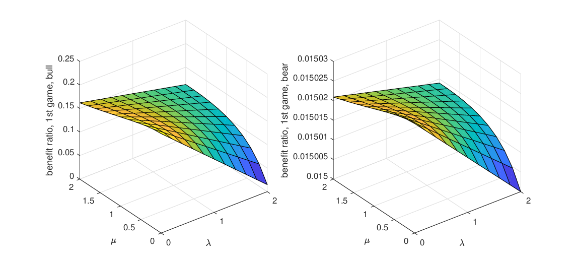
Refer to caption
Figure 2. Benefit ratio P^∗x\frac{\hat{P}_{*}}{x} in first game, bull and bear, γ=δ=2\gamma=\delta=2.

Previously, we suppose that the firm and the union have the same aversion parameters. In this paper, we are mainly interested in the effects of model uncertainty on the players’ behaviours. Next, we set γ=δ=2\gamma=\delta=2 and study the impacts of the firm’s and union’s ambiguity aversion parameters separately. Fig. 2 reveals that in the first game, no matter in a bull or bear market, the benefit ratio decreases with the union’s ambiguity aversion parameter λ\lambda while increases first and then decreases with the firm’s ambiguity aversion parameter μ\mu, see Eq. (4.24). Besides, when μ\mu increases, the benefit ratio is less sensitive to λ\lambda. It is also natural that the benefit ratio in the bear market is still lower that in the bull market.
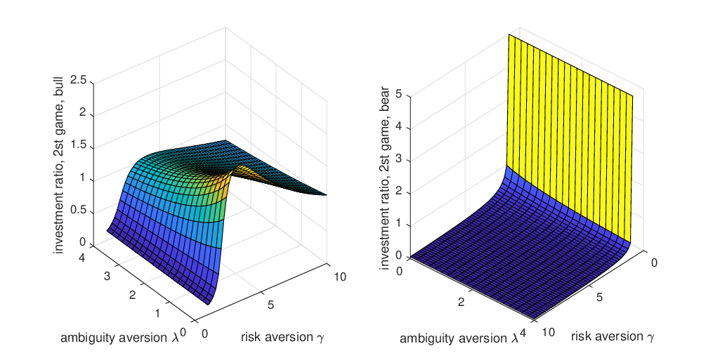
Refer to caption
Figure 3. Proportion of fund π^∗x\frac{\hat{\pi}_{*}}{x} invested in the risky asset in the second game, bull and bear.

Fig. 3 shows that the evolution of investment ratio has a similar pattern with the benefit ratio in the second game shown in Fig. 1(c) and Fig. 1(d). The impact of the risk aversion parameter γ\gamma on the investment strategy is larger than the ambiguity aversion parameter λ\lambda. When γ\gamma increases, the investment ratio increases rapidly to the highest point and then decreases slowly in the bull market. Meanwhile, the investment ratio is a decreasing function of λ\lambda. However, in the bear market, the effect of γ\gamma is much larger than that of λ\lambda. When γ\gamma increases, the investment strategy decreases rapidly to around zero.

In fact, these two types of aversion parameters of the union always indirectly affect the firm’s investment strategy π^∗x\frac{\hat{\pi}_{*}}{x} through the benefit ratio P^∗x\frac{\hat{P}_{*}}{x}. When the benefits claimed by the union increase, the firm will increase risky allocation to achieve high returns to ensure the stability of the fund surplus. As such, the evolution of the investment strategy is similar with the benefit ratio in the second game.

Comparing the two sub-figures in Fig. 3, we find that when γ\gamma is low, the investment ratio in the bear market is higher than that in the bull market. However, the conclusion is opposite when the risk aversion coefficient γ\gamma is relatively high. When the economy is in recession and the union has low risk aversion, the benefit ratio is high relatively to the risk-free interest rate. As such, the fund surplus may always be above the lower level. In order to reach the upper level, the firm will adopt a much more aggressive investment strategy. On the other hand, if the union has high risk aversion, then the benefit ratio becomes close to rr, as such, the investment strategy decreases.

6. Conclusion

In this paper, we investigate the overfunded DB pension plan game proposed in
Josa-Fombellida and Rincón-Zapatero, 2019. The firm manages the fund surplus and invests in the financial market while the pension fund participants claim part of the fund surplus as additional benefits. Different from Josa-Fombellida and Rincón-Zapatero, 2019, we assume that both the firm and the union are ambiguity aversion and consider two robust stochastic non-zero-sum games for them. The aims of the firm and the union are to searching the robust equilibrium strategies under worst case scenario.

In this first game, both players maximize their expected discounted utility under worst case scenario. However, in the second game, the firm aims to minimize the probability of the fund surplus reaching a low level. Using stochastic dynamic programming method, we obtain the explicit forms of the robust equilibrium strategies, the value functions and worst case measures. Particularly, in the first game, when the firm and the union have the same aversion parameters, the robust equilibrium strategy is Pareto optimal. We also see that the robust equilibrium strategies are proportional to the fund surplus in these two games. Besides, the robust investment strategy of the firm in the first game is only related to the risk aversion and ambiguity aversion of the firm. However, in the second game, the robust investment strategy only depends on the risk aversion and ambiguity aversion of the union. Finally, we present sensitivity analysis to reveal the player’s economic behaviors. Ambiguity aversion always prompts the union to adopt a more conservative strategy whether the economy is booming or sluggish, but this effect is smaller when the economy is in recession.

On the one hand, the robust optimal strategy in our work can provide a guidance to the firm and the union in practice to manage risk of model uncertainty. On the other hand, different from many previous work, we replace the uniform integrability condition by another condition, which is useful in proving the verification theorem of robust control problem.

Acknowledgements. The authors acknowledge the support from the National Natural Science Foundation of China (Grant No.11901574, No.11871036, and No.11471183). The authors also thank the members of the group of Mathematical Finance and Actuarial Science at the Department of Mathematical Sciences, Tsinghua University for their feedbacks and useful conversations.

Appendix A Proof of Theorem 4.2.

Proof.

Based on Remarks 3 and 3.7, we guess that the solutions of the HJBI equations (4.2)-(4.3) have the forms:

(A.1) WU​(s,x)=e−α​s​WU​(x),WF​(s,x)=e−β​s​WF​(x),W^{U}\left(s,x\right)=e^{-\alpha s}W^{U}\left(x\right),W^{F}\left(s,x\right)=e^{-\beta s}W^{F}\left(x\right),

with the properties

(A.2) (1−γ)​WU​(x)>0,(1−δ)​WF​(x)>0.\left(1-\gamma\right)W^{U}\left(x\right)>0,\quad\left(1-\delta\right)W^{F}\left(x\right)>0.

By using Eq. (A.1), the HJBI equations are rewritten as follows:

(A.3) 0\displaystyle 0 =\displaystyle= supP^infh^U{−αWU(x)+(rx+π^T(b−r1→)−P^−π^Tσh^U)WxU(x)\displaystyle\sup_{\hat{P}}\inf_{\hat{h}_{U}}\{-\alpha W^{U}\left(x\right)+\left(rx+\hat{\pi}^{T}\left(b-r\vec{1}\right)-\hat{P}-\hat{\pi}^{T}\sigma\hat{h}_{U}\right)W^{U}_{x}\left(x\right)
+12π^TΣπ^Wx​xU(x)+P^1−γ1−γ+(1−γ)h^UT​h^U2​λWU(x)},\displaystyle+\frac{1}{2}\hat{\pi}^{T}\Sigma\hat{\pi}W^{U}_{xx}\left(x\right)+\frac{\hat{P}^{1-\gamma}}{1-\gamma}+\left(1-\gamma\right)\frac{\hat{h}_{U}^{T}\hat{h}_{U}}{2\lambda}W^{U}\left(x\right)\},
(A.4) 0\displaystyle 0 =\displaystyle= supπ^infh^F{−βWF(x)+(rx+π^T(b−r1→)−P^−π^Tσh^F)WxF(x)\displaystyle\sup_{\hat{\pi}}\inf_{\hat{h}_{F}}\{-\beta W^{F}\left(x\right)+\left(rx+\hat{\pi}^{T}\left(b-r\vec{1}\right)-\hat{P}-\hat{\pi}^{T}\sigma\hat{h}_{F}\right)W^{F}_{x}\left(x\right)
+12π^TΣπ^Wx​xF(x)+x1−δ1−δ+(1−δ)h^FT​h^F2​μWF(x)}.\displaystyle+\frac{1}{2}\hat{\pi}^{T}\Sigma\hat{\pi}W^{F}_{xx}\left(x\right)+\frac{x^{1-\delta}}{1-\delta}+\left(1-\delta\right)\frac{\hat{h}_{F}^{T}\hat{h}_{F}}{2\mu}W^{F}\left(x\right)\}.

Using Eq. (A.2), we know that the function on the right side of Eq. (A.3) is an open-up quadratic function of h^U\hat{h}_{U}. As such, the first-order condition is

(A.5) h^U∗=λ​σT​π^​WxU​(x)(1−γ)​WU​(x).\hat{h}_{U*}=\frac{\lambda\sigma^{T}\hat{\pi}W_{x}^{U}\left(x\right)}{\left(1-\gamma\right)W^{U}\left(x\right)}.

Denote the right side of Eq. (A.3) by f1​(P^)f_{1}\left(\hat{P}\right), then we have f1′=P^−γ−WxU(x)f_{1}^{{}^{\prime}}=\hat{P}^{-\gamma}-W_{x}^{U}\left(x\right) and f1′′=−γP^−1−γ<0f_{1}^{{}^{\prime\prime}}=-\gamma\hat{P}^{-1-\gamma}<0, as such,

(A.6) P^∗=(WxU​(x))−1γ.\hat{P}_{*}=\left(W_{x}^{U}\left(x\right)\right)^{-\frac{1}{\gamma}}.

Similarly, if Eq. (A.2) holds, when

(A.7) h^F∗=μ​σT​π^​WxF​(x)(1−δ)​WF​(x),\hat{h}_{F*}=\frac{\mu\sigma^{T}\hat{\pi}W_{x}^{F}\left(x\right)}{\left(1-\delta\right)W^{F}\left(x\right)},

the right side of Eq. (A.4), i.e., f2​(π^)f_{2}\left(\hat{\pi}\right) attains the minimum and is

f2​(π^)\displaystyle f_{2}\left(\hat{\pi}\right) =\displaystyle= −β​WF​(x)+(r​x+π^T​(b−r​1→)−P^)​WxF​(x)\displaystyle-\beta W^{F}\left(x\right)+\left(rx+\hat{\pi}^{T}\left(b-r\vec{1}\right)-\hat{P}\right)W^{F}_{x}\left(x\right)
+12​π^T​Σ​π^​Wx​xF​(x)+x1−δ1−δ−μ​π^T​Σ​π^​(WxF​(x))22​(1−δ)​WF​(x).\displaystyle+\frac{1}{2}\hat{\pi}^{T}\Sigma\hat{\pi}W^{F}_{xx}\left(x\right)+\frac{x^{1-\delta}}{1-\delta}-\frac{\mu\hat{\pi}^{T}\Sigma\hat{\pi}\left(W_{x}^{F}\left(x\right)\right)^{2}}{2\left(1-\delta\right)W^{F}\left(x\right)}.

As such,

∇f2=(b−r​1→)​WxF​(x)−[μ​(WxF​(x))2(1−δ)​WF​(x)−Wx​xF​(x)]​Σ​π^.\nabla f_{2}=\left(b-r\vec{1}\right)W_{x}^{F}\left(x\right)-\left[\frac{\mu\left(W_{x}^{F}\left(x\right)\right)^{2}}{\left(1-\delta\right)W^{F}\left(x\right)}-W_{xx}^{F}\left(x\right)\right]\Sigma\hat{\pi}.

If

(A.8) D≜μ​(WxF​(x))2(1−δ)​WF​(x)−Wx​xF​(x)>0,D\triangleq\frac{\mu\left(W_{x}^{F}\left(x\right)\right)^{2}}{\left(1-\delta\right)W^{F}\left(x\right)}-W_{xx}^{F}\left(x\right)>0,

then

∇2f2=−D​Σ≺0.\nabla^{2}f_{2}=-D\Sigma\prec 0.

Thus,

(A.9) π^∗=Σ−1​(b−r​1→)​WxF​(x)D.\hat{\pi}_{*}=\frac{\Sigma^{-1}\left(b-r\vec{1}\right)W_{x}^{F}\left(x\right)}{D}.

Substituting Eq. (A.9) into Eqs. (A.5) and (A.7) yields

(A.10) h^U∗\displaystyle\hat{h}_{U*} =\displaystyle= λ​θ​WxU​(x)​WxF​(x)(1−γ)​WU​(x)​D,\displaystyle\frac{\lambda\theta W_{x}^{U}\left(x\right)W_{x}^{F}\left(x\right)}{\left(1-\gamma\right)W^{U}\left(x\right)D},
(A.11) h^F∗\displaystyle\hat{h}_{F*} =\displaystyle= μ​θ​(WxF​(x))2(1−δ)​WF​(x)​D.\displaystyle\frac{\mu\theta\left(W_{x}^{F}\left(x\right)\right)^{2}}{\left(1-\delta\right)W^{F}\left(x\right)D}.

Substituting Eqs. (A.6), (A.9), (A.10) and (A.11) into Eqs. (A.3) and (A.4), we obtain

(A.12) 0\displaystyle 0 =\displaystyle= −α​WU​(x)+γ1−γ​(WxU​(x))1−1γ+r​x​WxU​(x)\displaystyle-\alpha W^{U}\left(x\right)+\frac{\gamma}{1-\gamma}\left(W_{x}^{U}\left(x\right)\right)^{1-\frac{1}{\gamma}}+rxW_{x}^{U}\left(x\right)
+θT​θ​WxU​(x)​WxF​(x)D+12​θT​θ​(WxF​(x))2D2​Wx​xU​(x)\displaystyle+\theta^{T}\theta\frac{W_{x}^{U}\left(x\right)W_{x}^{F}\left(x\right)}{D}+\frac{1}{2}\theta^{T}\theta\frac{\left(W_{x}^{F}\left(x\right)\right)^{2}}{D^{2}}W_{xx}^{U}\left(x\right)
−θT​θ​λ2​(1−γ)​WU​(x)​(WxU​(x)​WxF​(x)D)2,\displaystyle-\theta^{T}\theta\frac{\lambda}{2\left(1-\gamma\right)W^{U}\left(x\right)}\left(\frac{W_{x}^{U}\left(x\right)W_{x}^{F}\left(x\right)}{D}\right)^{2},
(A.13) 0\displaystyle 0 =\displaystyle= −β​WF​(x)+x1−δ1−δ+r​x​WxF​(x)+θT​θ​(WxU​F​(x))2D\displaystyle-\beta W^{F}\left(x\right)+\frac{x^{1-\delta}}{1-\delta}+rxW_{x}^{F}\left(x\right)+\theta^{T}\theta\frac{\left(W_{x}^{U}F\left(x\right)\right)^{2}}{D}
−(WxU​(x))−1γ​WxF​(x)+12​θT​θ​(WxF​(x))2D2​Wx​xF​(x)\displaystyle-\left(W_{x}^{U}\left(x\right)\right)^{-\frac{1}{\gamma}}W_{x}^{F}\left(x\right)+\frac{1}{2}\theta^{T}\theta\frac{\left(W_{x}^{F}\left(x\right)\right)^{2}}{D^{2}}W_{xx}^{F}\left(x\right)
−θT​θ​μ2​(1−δ)​WF​(x)​((WxF​(x)2)D)2.\displaystyle-\theta^{T}\theta\frac{\mu}{2\left(1-\delta\right)W^{F}\left(x\right)}\left(\frac{\left(W_{x}^{F}\left(x\right)^{2}\right)}{D}\right)^{2}.

Suppose WU​(x)=A​x1−γ1−γW^{U}\left(x\right)=A\frac{x^{1-\gamma}}{1-\gamma}, WF​(x)=B​x1−δ1−δW^{F}\left(x\right)=B\frac{x^{1-\delta}}{1-\delta}, where AA and BB are some constants. In this case, Eq. (A.2) is equivalent to A>0A>0 and B>0B>0. As D=(μ+δ)​B​x−1−δ>0D=\left(\mu+\delta\right)Bx^{-1-\delta}>0 and Eq. (A.8) holds, Eqs. (A.12) and (A.13) are rewritten as follows:

0\displaystyle 0 =\displaystyle= −α1−γ​x1−γ​A+γ1−γ​x1−γ​A1−1γ+r​x1−γ​A\displaystyle-\frac{\alpha}{1-\gamma}x^{1-\gamma}A+\frac{\gamma}{1-\gamma}x^{1-\gamma}A^{1-\frac{1}{\gamma}}+rx^{1-\gamma}A
+θT​θμ+δ​x1−γ​A−θT​θ​γ2​(μ+δ)2​x1−γ​A−θT​θ​λ2​(μ+δ)2​x1−γ​A,\displaystyle+\frac{\theta^{T}\theta}{\mu+\delta}x^{1-\gamma}A-\theta^{T}\theta\frac{\gamma}{2\left(\mu+\delta\right)^{2}}x^{1-\gamma}A-\theta^{T}\theta\frac{\lambda}{2\left(\mu+\delta\right)^{2}}x^{1-\gamma}A,
0\displaystyle 0 =\displaystyle= −β1−δ​x1−δ​B+11−δ​x1−δ+r​x1−δ​B+θT​θμ+δ​x1−δ​B\displaystyle-\frac{\beta}{1-\delta}x^{1-\delta}B+\frac{1}{1-\delta}x^{1-\delta}+rx^{1-\delta}B+\frac{\theta^{T}\theta}{\mu+\delta}x^{1-\delta}B
−A−1γ​x1−δ​B−θT​θ​δ2​(μ+δ)2​x1−δ​B−θT​θ​μ2​(μ+δ)2​x1−δ​B,\displaystyle-A^{-\frac{1}{\gamma}}x^{1-\delta}B-\theta^{T}\theta\frac{\delta}{2\left(\mu+\delta\right)^{2}}x^{1-\delta}B-\theta^{T}\theta\frac{\mu}{2\left(\mu+\delta\right)^{2}}x^{1-\delta}B,

which are Eqs. (4.10) and (4.11) in Theorem 4.2.

Therefore, Eqs. (4.4) and (4.5) are the C1,2C^{1,2} solutions of the HJBI equations. Substituting the expressions WU​(x)=A​x1−γ1−γW^{U}\left(x\right)=A\frac{x^{1-\gamma}}{1-\gamma} and WF​(x)=B​x1−δ1−δW^{F}\left(x\right)=B\frac{x^{1-\delta}}{1-\delta} into Eqs. (A.6), (A.10), (A.9) and (A.11), we obtain Eqs. (4.6), (4.7), (4.8) and (4.9), correspondingly. ∎

Appendix B Proof of Lemma 4.3.

First, we present the following lemma about the geometric Brownian motion.

Lemma B.1.

Let {B⁡(t):t≥0}\left\{B\left(t\right):t\geq 0\right\} be an nn-dimensional standard Brownian motion, cc and mm are constants, and v∈𝐑nv\in\mathbf{R}^{n}. If the process {N⁡(t):t≥0}\left\{N\left(t\right):t\geq 0\right\} satisfies the stochastic differential equation d​N​(t)=c​N​(t)​d​t+N⁡(t)​vT​d​B​(t)\mathrm{d}N\left(t\right)=cN\left(t\right)\mathrm{d}t+N\left(t\right)v^{T}\mathrm{d}B(t), then N⁡(t)=N⁡(0)​exp⁡{(c−12​vT​v)​t+vT​B​(t)}N\left(t\right)=N\left(0\right)\exp\left\{\left(c-\frac{1}{2}v^{T}v\right)t+v^{T}B\left(t\right)\right\}. Moreover, if N⁡(0)N\left(0\right) and B⁡(t)B\left(t\right) are independent, then 𝐄​N​(t)m=𝐄⁡{N​(0)m​exp⁡{m⁡(c−12​vT​v)​t+12​m2​vT​v​t}}\mathbf{E}N\left(t\right)^{m}=\mathbf{E}\left\{N\left(0\right)^{m}\exp\left\{m\left(c-\frac{1}{2}v^{T}v\right)t+\frac{1}{2}m^{2}v^{T}vt\right\}\right\}.

Proof.

As {N⁡(t):t≥0}\{N\left(t\right):t\geq 0\} is a geometric Brownian motion, the explicit form of N⁡(t)N\left(t\right) can be easily derived by applying Itô’s formula to ln⁡N⁡(t)\ln N\left(t\right). Because {exp⁡{m​vT​B​(t)−12​m2​vT​v​t}:t≥0}\left\{\exp\left\{mv^{T}B\left(t\right)-\frac{1}{2}m^{2}v^{T}vt\right\}:t\geq 0\right\} is a martingale, we have

𝐄​N​(t)m\displaystyle\mathbf{E}N\left(t\right)^{m} =\displaystyle= 𝐄​N​(0)m​exp⁡{m⁡(c−12​vT​v)​t}+𝐄​exp⁡{m​vT​B​(t)}\displaystyle\mathbf{E}N\left(0\right)^{m}\exp\left\{m\left(c-\frac{1}{2}v^{T}v\right)t\right\}+\mathbf{E}\exp\left\{mv^{T}B\left(t\right)\right\}
=\displaystyle= 𝐄​N​(0)m​exp⁡{m⁡(c−12​vT​v)​t+12​m2​vT​v​t}.\displaystyle\mathbf{E}N\left(0\right)^{m}\exp\left\{m\left(c-\frac{1}{2}v^{T}v\right)t+\frac{1}{2}m^{2}v^{T}vt\right\}.

∎

Next, we prove Lemma 4.3 as follows:

Proof.

As XX satisfies the following SDE:

d​X​(t)\displaystyle\mathrm{d}X\left(t\right) =\displaystyle= X⁡(t)​(r+θT​θμ+δ−A−1γ)​d​t+X⁡(t)​1μ+δ​θT​d​W​(t)\displaystyle X\left(t\right)\left(r+\frac{\theta^{T}\theta}{\mu+\delta}-A^{-\frac{1}{\gamma}}\right)\mathrm{d}t+X\left(t\right)\frac{1}{\mu+\delta}\theta^{T}\mathrm{d}W\left(t\right)
=\displaystyle= X⁡(t)​(r+θT​θμ+δ−A−1γ−θT​θ​λ(μ+δ)2)​d​t+X⁡(t)​1μ+δ​θT​d​WhU∗​(t)\displaystyle X\left(t\right)\left(r+\frac{\theta^{T}\theta}{\mu+\delta}-A^{-\frac{1}{\gamma}}-\theta^{T}\theta\frac{\lambda}{\left(\mu+\delta\right)^{2}}\right)\mathrm{d}t+X\left(t\right)\frac{1}{\mu+\delta}\theta^{T}\mathrm{d}W^{h_{U}^{*}}\left(t\right)
=\displaystyle= X⁡(t)​(r+θT​θμ+δ−A−1γ−θT​θ​μ(μ+δ)2)​d​t+X⁡(t)​1μ+δ​θT​d​WhF∗​(t).\displaystyle X\left(t\right)\left(r+\frac{\theta^{T}\theta}{\mu+\delta}-A^{-\frac{1}{\gamma}}-\theta^{T}\theta\frac{\mu}{\left(\mu+\delta\right)^{2}}\right)\mathrm{d}t+X\left(t\right)\frac{1}{\mu+\delta}\theta^{T}\mathrm{d}W^{h_{F}^{*}}\left(t\right).

Based on Lemma B.1, we have

(B.1) X∗​(t)\displaystyle X^{*}\left(t\right)\!\!\! =\displaystyle= x​exp⁡{(r+θT​θμ+δ−A−1γ−θT​θ2​(μ+δ)2)​(t−s)+1μ+δ​θT​(W⁡(t)−W⁡(s))}\displaystyle\!\!\!\!\!x\!\exp\left\{\left(r+\frac{\theta^{T}\theta}{\mu+\delta}-A^{-\frac{1}{\gamma}}-\frac{\theta^{T}\theta}{2\left(\mu+\delta\right)^{2}}\right)\left(t-s\right)+\frac{1}{\mu+\delta}\theta^{T}\left(W\left(t\right)-W\left(s\right)\right)\right\}
=\displaystyle= x​exp⁡{(r+θT​θμ+δ−A−1γ−θT​θ​λ(μ+δ)2−θT​θ(μ+δ)2)​(t−s)+1μ+δ​θT​(WhU∗​(t)−WhU∗​(s))}\displaystyle\!\!\!x\!\exp\left\{\left(r\!+\!\frac{\theta^{T}\theta}{\mu+\delta}\!-\!A^{-\frac{1}{\gamma}}\!-\!\theta^{T}\theta\frac{\lambda}{\left(\mu\!+\!\delta\right)^{2}}\!-\!\frac{\theta^{T}\theta}{2\!\left(\mu\!+\!\delta\right)^{2}}\!\right)\left(t\!\!-\!\!s\right)\!+\!\frac{1}{\mu\!+\!\delta}\theta^{T}\!\left(\!W^{h_{U}^{*}}\left(t\right)\!-\!W^{h_{U}^{*}}\left(s\right)\!\right)\right\}
=\displaystyle= x​exp⁡{(r+θT​θμ+δ−A−1γ−θT​θ​μ(μ+δ)2−θT​θ2​(μ+δ)2)​(t−s)+1μ+δ​θT​(WhF∗​(t)−WhF∗​(s))}.\displaystyle\!\!\!\!x\!\exp\!\left\{\left(\!r\!+\!\!\frac{\theta^{T}\theta}{\mu\!+\!\delta}\!-\!\!A^{-\frac{1}{\gamma}}\!-\!\theta^{T}\theta\frac{\mu}{\left(\mu\!+\!\delta\right)^{2}}\!-\!\frac{\theta^{T}\theta}{2\left(\mu\!+\!\delta\right)^{2}}\right)\!\left(\!t\!\!-\!\!s\right)\!+\!\frac{1}{\mu\!+\!\delta}\theta^{T}\left(W^{h_{F}^{*}}\left(t\right)\!-\!W^{h_{F}^{*}}\left(s\right)\!\right)\!\!\right\}.

∎

Appendix C Proof of Lemma 4.4.

Proof.

As (π^∗,P^∗)\left(\hat{\pi}_{*},\hat{P}_{*}\right) is continuous, the process (π∗,P∗)=(π^∗​(X∗),P^∗​(X∗))\left(\pi_{*},P_{*}\right)=\left(\hat{\pi}_{*}\left(X^{*}\right),\hat{P}_{*}\left(X^{*}\right)\right) is adapted to the filtration {ℱt}t≥s\{\mathcal{F}_{t}\}_{t\geq s}. Under the strategy (π∗,P∗)\left(\pi_{*},P_{*}\right), SDE (2.3) has a pathwise unique solutions X∗X^{*}. Based on the expression of X∗X^{*} given by Eq. (B.1), we know X∗(t)>0,∀t≥s,ℙ-a.s.(ℚhU∗-a.s.,ℚhF∗-a.s.)X^{*}\left(t\right)>0,\ \forall\ t\geq s,\mathbb{P}\text{-a.s.}\left(\mathbb{Q}^{h_{U}^{*}}\text{-a.s.},\mathbb{Q}^{h_{F}^{*}}\text{-a.s.}\right). As such, we have π∗​(t)>0\pi_{*}\left(t\right)>0, P∗​(t)>0P_{*}\left(t\right)>0, ∀\forall t≥st\geq s, ℙ​-a.s.\mathbb{P}\text{-a.s.} (ℚhU∗​-a.s.,ℚhF∗​-a.s.\mathbb{Q}^{h_{U}^{*}}\text{-a.s.},\mathbb{Q}^{h_{F}^{*}}\text{-a.s.}). Therefore (π∗,P∗)∈Λ\left(\pi_{*},P_{*}\right)\in\Lambda. Noting that hU∗h_{U}^{*} and hF∗h_{F}^{*} are constant processes, Condition (i) in Definition 4.3 holds. Based on Lemma B.1, we have

𝐄s,xhU∗​{(X⁡(t))1−γ}\displaystyle{\mathbf{E}_{s,x}^{h_{U}^{*}}\left\{\left(X\left(t\right)\right)^{1-\gamma}\right\}} =\displaystyle= x1−γ​exp⁡{(1−γ)​(r+θT​θμ+δ−A−1γ−θT​θ​λ+γ(μ+δ)2)​(t−s)},\displaystyle x^{1-\gamma}\;\exp\left\{\left(1-\gamma\right)\left(r+\frac{\theta^{T}\theta}{\mu+\delta}-A^{-\frac{1}{\gamma}}-\theta^{T}\theta\frac{\lambda+\gamma}{\left(\mu+\delta\right)^{2}}\right)\left(t-s\right)\right\},
𝐄s,xhF∗​{(X⁡(t))1−δ}\displaystyle{\mathbf{E}_{s,x}^{h_{F}^{*}}\left\{\left(X\left(t\right)\right)^{1-\delta}\right\}} =\displaystyle= x1−δ​exp⁡{(1−δ)​(r+θT​θ2​(μ+δ)−A−1γ)​(t−s)}.\displaystyle x^{1-\delta}\;\exp\left\{\left(1-\delta\right)\left(r+\frac{\theta^{T}\theta}{2\left(\mu+\delta\right)}-A^{-\frac{1}{\gamma}}\right)\left(t-s\right)\right\}.

As such, Conditions (ii) and (iii) in Definition 4.3 hold if

(1−γ)​(r+θT​θμ+δ−A−1γ−θT​θ​λ+γ(μ+δ)2)<α,\displaystyle\left(1-\gamma\right)\left(r+\frac{\theta^{T}\theta}{\mu+\delta}-A^{-\frac{1}{\gamma}}-\theta^{T}\theta\frac{\lambda+\gamma}{\left(\mu+\delta\right)^{2}}\right)<\alpha,
(1−δ)​(r+θT​θ2​(μ+δ)−A−1γ)<β.\displaystyle\left(1-\delta\right)\left(r+\frac{\theta^{T}\theta}{2\left(\mu+\delta\right)}-A^{-\frac{1}{\gamma}}\right)<\beta.

The last two Ineqs. are equivalent to A>0A>0 and B>0B>0. In addition, Condition (iv) in Definition 4.3 is equivalent to

𝐄s,xhU∗​[∫sT(X⁡(t))2−2​γ​𝑑t]<∞,∀T≥s,\displaystyle\mathbf{E}_{s,x}^{h_{U}^{*}}\left[\int_{s}^{T}\left(X\left(t\right)\right)^{2-2\gamma}\mathrm{d}t\right]<\infty,\quad\forall T\geq s,
𝐄s,xhF∗​[∫sT(X⁡(t))2−2​δ​𝑑t]<∞,∀T≥s.\displaystyle\mathbf{E}_{s,x}^{h_{F}^{*}}\left[\int_{s}^{T}\left(X\left(t\right)\right)^{2-2\delta}\mathrm{d}t\right]<\infty,\quad\forall T\geq s.

Based on Lemma B.1, 𝐄s,xhU∗​{X⁡(t)}2−2​γ\mathbf{E}_{s,x}^{h_{U}^{*}}\left\{X\left(t\right)\right\}^{2-2\gamma} and 𝐄s,xhF∗​{X⁡(t)}2−2​δ\mathbf{E}_{s,x}^{h_{F}^{*}}\left\{X\left(t\right)\right\}^{2-2\delta} can be written in the form of C1​eC2​(t−s)C_{1}e^{C_{2}\left(t-s\right)}, as such, Condition (iv) holds. Thus, hU∗∈ℋU​(π∗,P∗)h_{U}^{*}\in\mathcal{H}_{U}\left(\pi_{*},P_{*}\right) and hF∗∈ℋF​(π∗,P∗)h_{F}^{*}\in\mathcal{H}_{F}\left(\pi_{*},P_{*}\right) follow. ∎

Appendix D Proof of Lemma 4.6.

Proof.

Based on the forms of HJBI equations (4.2)\left(\ref{hjbfc1}\right) and (4.3)\left(\ref{hjbcf2}\right) with variable (s,x)∈𝐑+2\left(s,x\right)\in\mathbb{\mathbf{R}}_{+}^{2}, it is easy to see that the properties (i) and(iii) hold. Property (iv) is exactly equivalent to Condition (iii) in Definition 4.3 with variable (s,x)∈𝐑+2\left(s,x\right)\in\mathbf{R}_{+}^{2}, which is naturally satisfied.

As the function involved in P^\hat{P} does not depend on π^\hat{\pi} and h^U\hat{h}_{U}, the first formula of Property (ii) is easily verified by Eq. (4.2). Next, we verify the second one. Let f3(π^)≜𝒜π^,P^∗,h^F∗WF(t,y)+ΦF(t,y,π^,P^∗,h^F∗,WF)f_{3}\left(\hat{\pi}\right)\triangleq\mathcal{A}^{\hat{\pi},\hat{P}_{*},\hat{h}_{F*}}W_{F}\left(t,y\right)+\Phi^{F}\left(t,y,\hat{\pi},\hat{P}_{*},\hat{h}_{F*},W^{F}\right). Then we obtain the derivatives of f3f_{3}:

∇f3\displaystyle\nabla f_{3} =\displaystyle= e−α​t​((b−r​1→)​WxF​(y)−μμ+δ​σ​θ−Σ​π^​Wx​xF​(y))\displaystyle e^{-\alpha t}\left(\left(b-r\vec{1}\right)W_{x}^{F}\left(y\right)-\frac{\mu}{\mu+\delta}\sigma\theta-\Sigma\hat{\pi}W_{xx}^{F}\left(y\right)\right)
=\displaystyle= e−α​t​δ​B​y−δ​((b−r​1→)μ+δ−y−1​Σ​π^),\displaystyle e^{-\alpha t}\delta By^{-\delta}\left(\frac{\left(b-r\vec{1}\right)}{\mu+\delta}-y^{-1}\Sigma\hat{\pi}\right),
∇2f3\displaystyle\nabla^{2}f_{3} =\displaystyle= −e−α​t​δ​B​y−δ−1​Σ≺0.\displaystyle-e^{-\alpha t}\delta By^{-\delta-1}\Sigma\prec 0.

As such, if π^=1μ+δ​Σ−1​(b−r​1→)​y=π^∗​(y)\hat{\pi}=\frac{1}{\mu+\delta}\Sigma^{-1}\left(b-r\vec{1}\right)y=\hat{\pi}_{*}\left(y\right), then ∇f3=0\nabla f_{3}=0. Thus , f3​(π^)≤f3​(π^∗​(y))=0f_{3}\left(\hat{\pi}\right)\leq f_{3}\left(\hat{\pi}_{*}\left(y\right)\right)=0. ∎

Appendix E Proof of Theorem 4.30.

Proof.

Suppose that the solution of the HJBI equation (4.29) has properties

(E.1) W0​(s,x)=e−α​s​W0​(x),(1−γ)​W0​(x)>0.W^{0}\left(s,x\right)=e^{-\alpha s}W^{0}\left(x\right),\quad\left(1-\gamma\right)W^{0}\left(x\right)>0.

Then the HJBI equation is rewritten as follows:

(E.2) 0\displaystyle 0 =\displaystyle= supπ^,P^infh^0{−αW0(x)+(rx+π^T(b−r1→)−P^−π^Tσh^0)Wx0(x)\displaystyle\sup_{\hat{\pi},\hat{P}}\inf_{\hat{h}_{0}}\left\{-\alpha W^{0}\left(x\right)+\left(rx+\hat{\pi}^{T}\left(b-r\vec{1}\right)-\hat{P}-\hat{\pi}^{T}\sigma\hat{h}_{0}\right)W^{0}_{x}\left(x\right)\right.
+12π^TΣπ^Wx​x0(x)+P^1−γ1−γ+(1−γ)h^0T​h^02​λW0(x)}.\displaystyle+\left.\frac{1}{2}\hat{\pi}^{T}\Sigma\hat{\pi}W^{0}_{xx}\left(x\right)+\frac{\hat{P}^{1-\gamma}}{1-\gamma}+\left(1-\gamma\right)\frac{\hat{h}_{0}^{T}\hat{h}_{0}}{2\lambda}W^{0}\left(x\right)\right\}.

Following the proof of Theorem 4.2, we have

(E.3) h^0∗\displaystyle\hat{h}_{0*} =\displaystyle= λ​σT​π^​Wx0​(x)(1−γ)​W0​(x),\displaystyle\frac{\lambda\sigma^{T}\hat{\pi}W_{x}^{0}\left(x\right)}{\left(1-\gamma\right)W^{0}\left(x\right)},
(E.4) P0^∗\displaystyle\hat{P_{0}}_{*} =\displaystyle= (Wx0​(x))−1γ.\displaystyle\left(W_{x}^{0}\left(x\right)\right)^{-\frac{1}{\gamma}}.

As such, the right side of Eq. (E.2) is

f0​(π^)\displaystyle f_{0}\left(\hat{\pi}\right) =\displaystyle= −α​W0​(x)+(r​x+π^T​(b−r​1→)−P^0∗)​Wx0​(x)\displaystyle-\alpha W^{0}\left(x\right)+\left(rx+\hat{\pi}^{T}\left(b-r\vec{1}\right)-\hat{P}_{0}^{*}\right)W^{0}_{x}\left(x\right)
+12​π^T​Σ​π^​Wx​x0​(x)+(P0^∗)1−γ1−γ−λ​π^T​Σ​π^​(Wx0​(x))22​(1−γ)​W0​(x).\displaystyle+\frac{1}{2}\hat{\pi}^{T}\Sigma\hat{\pi}W^{0}_{xx}\left(x\right)+\frac{\left(\hat{P_{0}}_{*}\right)^{1-\gamma}}{1-\gamma}-\frac{\lambda\hat{\pi}^{T}\Sigma\hat{\pi}\left(W_{x}^{0}\left(x\right)\right)^{2}}{2\left(1-\gamma\right)W^{0}\left(x\right)}.

Similar to that of Theorem 4.2, we obtain that if

(E.5) D0≜λ​(Wx0​(x))2(1−γ)​W0​(x)−Wx​x0​(x)>0,D_{0}\triangleq\frac{\lambda\left(W_{x}^{0}\left(x\right)\right)^{2}}{\left(1-\gamma\right)W^{0}\left(x\right)}-W_{xx}^{0}\left(x\right)>0,

then

(E.6) π0^∗=Σ−1​(b−r​1→)​Wx0​(x)D0.\hat{\pi_{0}}_{*}=\frac{\Sigma^{-1}\left(b-r\vec{1}\right)W_{x}^{0}\left(x\right)}{D_{0}}.

As such, the HJBI equation becomes

(E.7) 0\displaystyle 0 =\displaystyle= −α​W0​(x)+γ1−γ​(Wx0​(x))1−1γ+r​x​Wx0​(x)\displaystyle-\alpha W^{0}\left(x\right)+\frac{\gamma}{1-\gamma}\left(W_{x}^{0}\left(x\right)\right)^{1-\frac{1}{\gamma}}+rxW_{x}^{0}\left(x\right)
+θT​θ​(Wx0​(x))2D0+12​θT​θ​(Wx0​(x))2D02​Wx​x0​(x)−θT​θ​λ​(W0​(x))42​(1−γ)​W0​(x)​D02.\displaystyle+\theta^{T}\theta\frac{\left(W_{x}^{0}\left(x\right)\right)^{2}}{D_{0}}+\frac{1}{2}\theta^{T}\theta\frac{\left(W_{x}^{0}\left(x\right)\right)^{2}}{D_{0}^{2}}W_{xx}^{0}\left(x\right)-\theta^{T}\theta\frac{\lambda\left(W^{0}\left(x\right)\right)^{4}}{2\left(1-\gamma\right)W^{0}\left(x\right)D_{0}^{2}}.

Solving Eq. (E.7) yields W0​(x)=A0​x1−γ1−γW^{0}\left(x\right)=A_{0}\frac{x^{1-\gamma}}{1-\gamma}, where A0A_{0} is given by Eq. (4.30). Noting that Assumption (E.1) is equivalent to A0>0A_{0}>0, Assumption (E.5) naturally holds. As such, (π0^∗,P0^∗)\left(\hat{\pi_{0}}_{*},\hat{P_{0}}_{*}\right) and h^0∗\hat{h}_{0*} are derived. Thus, the proof is completed. ∎

Appendix F Proof of Theorem 4.12.

Proof.

We guess that the solutions of the HJBI equations (4.31)-(4.32) have the forms:

(F.1) WU¯​(s,x)=e−α​s​WU¯​(x),WF¯​(s,x)=WF¯​(x).W^{\bar{U}}\left(s,x\right)=e^{-\alpha s}W^{\bar{U}}\left(x\right),\ \ \ W^{\bar{F}}\left(s,x\right)=W^{\bar{F}}\left(x\right).

Suppose that WU¯W^{\bar{U}} and WF¯W^{\bar{F}} satisfy

(F.2) (1−γ)​WU¯​(x)>0,WF¯​(x)>0.\left(1-\gamma\right)W^{\bar{U}}\left(x\right)>0,\quad W^{\bar{F}}\left(x\right)>0.

If Eqs. (F.1) and (F.2) hold, then the HJBI equations are equivalent to

(F.3) 0\displaystyle 0 =\displaystyle= supP^infh^U¯{−αWU¯(x)+(rx+π^T(b−r1→)−P^−π^Tσh^U¯)WxU¯(x)\displaystyle\sup_{\hat{P}}\inf_{\hat{h}_{\bar{U}}}\left\{-\alpha W^{\bar{U}}\left(x\right)+\left(rx+\hat{\pi}^{T}\left(b-r\vec{1}\right)-\hat{P}-\hat{\pi}^{T}\sigma\hat{h}_{\bar{U}}\right)W^{\bar{U}}_{x}\left(x\right)\right.
+12π^TΣπ^Wx​xU¯(x)+P^1−γ1−γ+(1−γ)h^U¯T​h^U¯2​λWU¯(x)},\displaystyle+\left.\frac{1}{2}\hat{\pi}^{T}\Sigma\hat{\pi}W^{\bar{U}}_{xx}\left(x\right)+\frac{\hat{P}^{1-\gamma}}{1-\gamma}+\left(1-\gamma\right)\frac{\hat{h}_{\bar{U}}^{T}\hat{h}_{\bar{U}}}{2\lambda}W^{\bar{U}}\left(x\right)\right\},
(F.4) 0\displaystyle 0 =\displaystyle= supπ^infh^F¯{(rx+π^T(b−r1→)−P^−π^Tσh^F¯)WxF¯(x)\displaystyle\sup_{\hat{\pi}}\inf_{\hat{h}_{\bar{F}}}\left\{\left(rx+\hat{\pi}^{T}\left(b-r\vec{1}\right)-\hat{P}-\hat{\pi}^{T}\sigma\hat{h}_{\bar{F}}\right)W^{\bar{F}}_{x}\left(x\right)\right.
+12π^TΣπ^Wx​xF¯(x)+h^F¯T​h^F¯2​μ(WF¯(x)+c)}.\displaystyle+\left.\frac{1}{2}\hat{\pi}^{T}\Sigma\hat{\pi}W^{\bar{F}}_{xx}\left(x\right)+\frac{\hat{h}_{\bar{F}}^{T}\hat{h}_{\bar{F}}}{2\mu}\left(W^{\bar{F}}\left(x\right)+c\right)\right\}.

Similar to that of Theorem 4.2, we know that the minimum point h^U∗\hat{h}_{U*} and the maximum P^∗\hat{P}_{*} are

(F.5) h^U∗=λ​σT​π^​WxU¯​(x)(1−γ)​WU¯​(x),\hat{h}_{U*}=\frac{\lambda\sigma^{T}\hat{\pi}W_{x}^{\bar{U}}\left(x\right)}{\left(1-\gamma\right)W^{\bar{U}}\left(x\right)},
(F.6) P^∗=(WxU¯​(x))−1γ.\hat{P}_{*}=\left(W_{x}^{\bar{U}}\left(x\right)\right)^{-\frac{1}{\gamma}}.

Combining Eqs. (F.4) and (F.2), we have that when

(F.7) h^F∗=μ​σT​π^​WxF¯​(x)WF¯​(x)+c,\hat{h}_{F*}=\frac{\mu\sigma^{T}\hat{\pi}W_{x}^{\bar{F}}\left(x\right)}{W^{\bar{F}}\left(x\right)+c},

the right side of the HJBI equation attains the minimum and becomes

f2​(π^)\displaystyle f_{2}\left(\hat{\pi}\right) =\displaystyle= (r​x+π^T​(b−r​1→)−P^)​WxF¯​(x)\displaystyle\left(rx+\hat{\pi}^{T}\left(b-r\vec{1}\right)-\hat{P}\right)W^{\bar{F}}_{x}\left(x\right)
+12​π^T​Σ​π^​Wx​xF¯​(x)−μ​π^T​Σ​π^​(WxF¯​(x))22​(WF¯​(x)+c),\displaystyle+\frac{1}{2}\hat{\pi}^{T}\Sigma\hat{\pi}W^{\bar{F}}_{xx}\left(x\right)-\frac{\mu\hat{\pi}^{T}\Sigma\hat{\pi}\left(W_{x}^{\bar{F}}\left(x\right)\right)^{2}}{2\left(W^{\bar{F}}\left(x\right)+c\right)},

with derivative

∇f2=(b−r​1→)​WxF¯​(x)−[μ​(WxF¯​(x))2WF¯​(x)+c−Wx​xF¯​(x)]​Σ​π^.\nabla f_{2}=\left(b-r\vec{1}\right)W_{x}^{\bar{F}}\left(x\right)-\left[\frac{\mu\left(W_{x}^{\bar{F}}\left(x\right)\right)^{2}}{W^{\bar{F}}\left(x\right)+c}-W_{xx}^{\bar{F}}\left(x\right)\right]\Sigma\hat{\pi}.

If we assume

(F.8) F≜μ​(WxF¯​(x))2WF¯​(x)+c−Wx​xF¯​(x)>0,F\triangleq\frac{\mu\left(W_{x}^{\bar{F}}\left(x\right)\right)^{2}}{W^{\bar{F}}\left(x\right)+c}-W_{xx}^{\bar{F}}\left(x\right)>0,

then

∇2f2=−F​Σ≺0.\nabla^{2}f_{2}=-F\Sigma\prec 0.

As such,

(F.9) π^∗=Σ−1​(b−r​1→)​WxF¯​(x)F.\hat{\pi}_{*}=\frac{\Sigma^{-1}\left(b-r\vec{1}\right)W_{x}^{\bar{F}}\left(x\right)}{F}.

Substituting Eq. (F.9) into Eqs. (F.5) and (F.7) yields

(F.10) h^U∗\displaystyle\hat{h}_{U*} =\displaystyle= λ​θ​WxU¯​(x)​WxF¯​(x)(1−γ)​WU¯​(x)​F,\displaystyle\frac{\lambda\theta W_{x}^{\bar{U}}\left(x\right)W_{x}^{\bar{F}}\left(x\right)}{\left(1-\gamma\right)W^{\bar{U}}\left(x\right)F},
(F.11) h^F∗\displaystyle\hat{h}_{F*} =\displaystyle= μ​θ​(WxF¯​(x))2(WF¯​(x)+c)​F.\displaystyle\frac{\mu\theta\left(W_{x}^{\bar{F}}\left(x\right)\right)^{2}}{\left(W^{\bar{F}}\left(x\right)+c\right)F}.

Substituting Eqs. (F.10), (F.6), (F.11) and (F.9) into Eqs. (F.3) and (F.4), we obtain

(F.12) 0\displaystyle 0 =\displaystyle= −α​WU¯​(x)+γ1−γ​(WxU¯​(x))1−1γ+r​x​WxU¯​(x)\displaystyle-\alpha W^{\bar{U}}\left(x\right)+\frac{\gamma}{1-\gamma}\left(W_{x}^{\bar{U}}\left(x\right)\right)^{1-\frac{1}{\gamma}}+rxW_{x}^{\bar{U}}\left(x\right)
+θT​θ​WxU¯​(x)​WxF¯​(x)F+12​θT​θ​(WxF¯​(x))2F2​Wx​xU¯​(x)\displaystyle+\theta^{T}\theta\frac{W_{x}^{\bar{U}}\left(x\right)W_{x}^{\bar{F}}\left(x\right)}{F}+\frac{1}{2}\theta^{T}\theta\frac{\left(W_{x}^{\bar{F}}\left(x\right)\right)^{2}}{F^{2}}W_{xx}^{\bar{U}}\left(x\right)
−θT​θ​λ2​(1−γ)​WU¯​(x)​(WxU¯​(x)​WxF¯​(x)F)2,\displaystyle-\theta^{T}\theta\frac{\lambda}{2\left(1-\gamma\right)W^{\bar{U}}\left(x\right)}\left(\frac{W_{x}^{\bar{U}}\left(x\right)W_{x}^{\bar{F}}\left(x\right)}{F}\right)^{2},
(F.13) 0\displaystyle 0 =\displaystyle= r​x​WxF¯​(x)+θT​θ​(WxU¯​F​(x))2F\displaystyle rxW_{x}^{\bar{F}}\left(x\right)+\theta^{T}\theta\frac{\left(W_{x}^{\bar{U}}F\left(x\right)\right)^{2}}{F}
−(WxU¯​(x))−1γ​WxF¯​(x)+12​θT​θ​(WxF¯​(x))2F2​Wx​xF¯​(x)\displaystyle-\left(W_{x}^{\bar{U}}\left(x\right)\right)^{-\frac{1}{\gamma}}W_{x}^{\bar{F}}\left(x\right)+\frac{1}{2}\theta^{T}\theta\frac{\left(W_{x}^{\bar{F}}\left(x\right)\right)^{2}}{F^{2}}W_{xx}^{\bar{F}}\left(x\right)
−θT​θ​μ2​(WF¯​(x)+c)​((WxF¯​(x)2)F)2.\displaystyle-\theta^{T}\theta\frac{\mu}{2\left(W^{\bar{F}}\left(x\right)+c\right)}\left(\frac{\left(W_{x}^{\bar{F}}\left(x\right)^{2}\right)}{F}\right)^{2}.

Finally, we only need to show that Eqs. (F.2) and (F.8) hold, and WU¯​(x)=E​x1−γ1−γW^{\bar{U}}\left(x\right)=E\frac{x^{1-\gamma}}{1-\gamma} and WF¯​(x)=x1−η−l1−ηv1−η−l1−ηW^{\bar{F}}\left(x\right)=\frac{x^{1-\eta}-l^{1-\eta}}{v^{1-\eta}-l^{1-\eta}} indeed solve Eqs (F.13)-(F.13). The first part of Eq. (F.2) is equivalent to E>0E>0 and the second part naturally holds. Using α>r\alpha>r, η<1\eta<1 and Eq. (4.34), we know μ⁡(1−η)+η=ω>0\mu\left(1-\eta\right)+\eta=\omega>0, then F=(1−η)​[μ⁡(1−η)+η]​x−1−ηv1−η−l1−η>0F=\left(1-\eta\right)\left[\mu\left(1-\eta\right)+\eta\right]\frac{x^{-1-\eta}}{v^{1-\eta}-l^{1-\eta}}>0. As such, Eq. (F.8) holds, and Eqs. (F.13)-(F.13) become

0\displaystyle 0 =\displaystyle= −α1−γ​x1−γ​E+γ1−γ​x1−γ​E1−1γ+r​x1−γ​E+θT​θμ⁡(1−η)+η​x1−γ​E\displaystyle-\frac{\alpha}{1-\gamma}x^{1-\gamma}E+\frac{\gamma}{1-\gamma}x^{1-\gamma}E^{1-\frac{1}{\gamma}}+rx^{1-\gamma}E+\frac{\theta^{T}\theta}{\mu\left(1-\eta\right)+\eta}x^{1-\gamma}E
−θT​θ​γ2​[μ⁡(1−η)+η]2​x1−γ​E−θT​θ​λ2​[μ⁡(1−η)+η]2​x1−γ​E,\displaystyle-\theta^{T}\theta\frac{\gamma}{2\left[\mu\left(1-\eta\right)+\eta\right]^{2}}x^{1-\gamma}E-\theta^{T}\theta\frac{\lambda}{2\left[\mu\left(1-\eta\right)+\eta\right]^{2}}x^{1-\gamma}E,
0\displaystyle 0 =\displaystyle= r⁡(1−η)​x1−ηv1−η−l1−η+θT​θ​1−ημ⁡(1−η)+η​x1−ηv1−η−l1−η−E−1γ​(1−η)​x1−ηv1−η−l1−η\displaystyle r\left(1-\eta\right)\frac{x^{1-\eta}}{v^{1-\eta}-l^{1-\eta}}+\theta^{T}\theta\frac{1-\eta}{\mu\left(1-\eta\right)+\eta}\frac{x^{1-\eta}}{v^{1-\eta}-l^{1-\eta}}-E^{-\frac{1}{\gamma}}\left(1-\eta\right)\frac{x^{1-\eta}}{v^{1-\eta}-l^{1-\eta}}
−θT​θ​η⁡(1−η)2​[μ⁡(1−η)+η]2​x1−ηv1−η−l1−η−θT​θ​μ2​[μ⁡(1−η)+η]2​x1−ηv1−η−l1−η.\displaystyle-\theta^{T}\theta\frac{\eta\left(1-\eta\right)}{2\left[\mu\left(1-\eta\right)+\eta\right]^{2}}\frac{x^{1-\eta}}{v^{1-\eta}-l^{1-\eta}}-\theta^{T}\theta\frac{\mu}{2\left[\mu\left(1-\eta\right)+\eta\right]^{2}}\frac{x^{1-\eta}}{v^{1-\eta}-l^{1-\eta}}.

Simplifying the last two equations,

(F.14) 0\displaystyle 0 =\displaystyle= −α1−γ+r+γ1−γ​E−1γ+θT​θμ⁡(1−η)+η−θT​θ​λ+γ2​[μ⁡(1−η)+η]2,\displaystyle-\frac{\alpha}{1-\gamma}+r+\frac{\gamma}{1-\gamma}E^{-\frac{1}{\gamma}}+\frac{\theta^{T}\theta}{\mu\left(1-\eta\right)+\eta}-\theta^{T}\theta\frac{\lambda+\gamma}{2\left[\mu\left(1-\eta\right)+\eta\right]^{2}},
(F.15) 0\displaystyle 0 =\displaystyle= r+θT​θ2​[μ​(1−η)+η]−E−1γ.\displaystyle r+\frac{\theta^{T}\theta}{2\left[\mu\left(1-\eta\right)+\eta\right]}-E^{-\frac{1}{\gamma}}.

Eq. (4.35) implies ω=μ⁡(1−η)+η\omega=\mu\left(1-\eta\right)+\eta. Therefore, Eq. (F.15) holds because of Eq. (4.34). Using Eqs. (4.33) and (4.34), Eq. (F.14) holds. ∎

Appendix G Proof of Lemma 4.13.

Proof.

Following the proof of Lemma 4.6, the properties (i), (ii), (iii) and the first part of (iv) can be proved. For the proof of the second part of property (ii), the condition η>0\eta>0 is required. As such, we only need to prove the second part of property (iv).

Noting X⁡(𝒯N)∈(l,v),∀NX\left(\mathcal{T}_{N}\right)\in\left(l,v\right),\forall N, we have supN𝐄s,xhF¯​|X⁡(𝒯N)|2<∞\sup\limits_{N}\mathbf{E}_{s,x}^{h_{\bar{F}}}|X\left(\mathcal{T}_{N}\right)|^{2}<\infty, which implies that
{X⁡(𝒯N):N≥0}\left\{X\left(\mathcal{T}_{N}\right):N\geq 0\right\} is uniformly integrable. As 𝒯<∞,ℚhF¯​-a.s.\mathcal{T}<\infty,\mathbb{Q}^{h_{\bar{F}}}\text{-a.s.}, and WF¯​(𝒯N,X⁡(𝒯N))→WF¯​(𝒯,X⁡(𝒯)),ℚhF¯​-a.s.W^{\bar{F}}\left(\mathcal{T}_{N},X\left(\mathcal{T}_{N}\right)\right)\rightarrow W^{\bar{F}}\left(\mathcal{T},X\left(\mathcal{T}\right)\right),\mathbb{Q}^{h_{\bar{F}}}\text{-a.s.}, we know that Eq. (4.38) holds. ∎

Appendix H Proof of Theorem 4.14.

Proof.

∀(π,P)∈Λ,hU¯∈ℋU¯​(π,P)\forall\ \left(\pi,P\right)\in\Lambda,\ h_{\bar{U}}\in\mathcal{H}_{\bar{U}}(\pi,P), let XX be the unique solution of SDE (2.3). Similar to the proof of Theorem 4.5, we have

infhU¯∈ℋU¯​(π∗,P∗)JU¯​(s,x,π∗,P∗,hU¯)\displaystyle\inf_{h_{\bar{U}}\in\mathcal{H}_{\bar{U}}\left(\pi_{*},P_{*}\right)}J_{\bar{U}}\left(s,x,\pi_{*},P_{*},h_{\bar{U}}\right) =\displaystyle= supP:(π∗,P)∈ΛinfhU¯∈ℋU¯​(π∗,P)JU¯(s,x,π∗,P,hU¯)\displaystyle\sup_{P:\left(\pi_{*},P\right)\in\Lambda}\inf_{h_{\bar{U}}\in\mathcal{H}_{\bar{U}}\left(\pi_{*},P\right)}J_{\bar{U}}\left(s,x,\pi_{*},P,h_{\bar{U}}\right)
=\displaystyle= VU¯π∗​(s,x)=WU¯​(s,x)=JU¯​(s,x,π∗,P∗,hU¯∗).\displaystyle V_{\bar{U}}^{\pi_{*}}\left(s,x\right)=W^{\bar{U}}\left(s,x\right)=J_{\bar{U}}\left(s,x,\pi_{*},P_{*},h_{\bar{U}}^{*}\right).

Thus, we only need to show

infhF¯∈ℋF¯​(π∗,P∗)JF¯​(s,x,π∗,P∗,hF¯)\displaystyle\inf_{h_{\bar{F}}\in\mathcal{H}_{\bar{F}}\left(\pi_{*},P_{*}\right)}J_{\bar{F}}\left(s,x,\pi_{*},P_{*},h_{\bar{F}}\right) =\displaystyle= supπ:(π,P∗)∈ΛinfhF¯∈ℋF¯​(π,P∗)JF¯(s,x,π,P∗,hF¯)\displaystyle\sup_{\pi:\left(\pi,P_{*}\right)\in\Lambda}\inf_{h_{\bar{F}}\in\mathcal{H}_{\bar{F}}\left(\pi,P_{*}\right)}J_{\bar{F}}\left(s,x,\pi,P_{*},h_{\bar{F}}\right)
=\displaystyle= VF¯P∗​(s,x)=WF¯​(s,x)=JF¯​(s,x,π∗,P∗,hF¯∗).\displaystyle V_{\bar{F}}^{P_{*}}\left(s,x\right)=W^{\bar{F}}\left(s,x\right)=J_{\bar{F}}\left(s,x,\pi_{*},P_{*},h_{\bar{F}}^{*}\right).

Using Itô’s formula, we have

WF¯​(𝒯,X⁡(𝒯))=WF¯​(s,X⁡(s))+∫s𝒯𝒜π,P,hF¯​WF¯​(t,X⁡(t))​𝑑t+∫s𝒯WxF¯​(t,X⁡(t))​π​(t)T​σ​d​WhF¯​(t).\displaystyle W^{\bar{F}}\left(\mathcal{T},X\left(\mathcal{T}\right)\right)=\!W^{\bar{F}}\left(s,X\left(s\right)\right)\!+\!\int_{s}^{\mathcal{T}}\mathcal{A}^{\pi,P,h_{\bar{F}}}W^{\bar{F}}\left(t,X\left(t\right)\right)\mathrm{d}t\!+\!\int_{s}^{\mathcal{T}}W_{x}^{\bar{F}}\left(t,X\left(t\right)\right)\pi\left(t\right)^{T}\sigma\!\mathrm{d}W^{h_{\bar{F}}}\left(t\right).

Let 𝒯N≜𝒯∧N∧inf{t>s;∫st|WxF¯(z,X(z))π(z)Tσ|2dz≥N}\mathcal{T}_{N}\triangleq\mathcal{T}\wedge N\wedge\inf\left\{t>s;\int_{s}^{t}|W_{x}^{\bar{F}}\left(z,X\left(z\right)\right)\pi\left(z\right)^{T}\sigma|^{2}\mathrm{d}z\geq N\right\}, then 𝒯N\mathcal{T}_{N} is a stopping time and {∫sT∧𝒯NWxF¯(t,X(t))π(t)TσdWhF¯(t);s≤T≤N}\left\{\int_{s}^{T\wedge\mathcal{T}_{N}}W_{x}^{\bar{F}}\left(t,X\left(t\right)\right)\pi\left(t\right)^{T}\sigma\mathrm{d}W^{h_{\bar{F}}}\left(t\right);s\leq T\leq N\right\} is a ℚhF¯\mathbb{Q}^{h_{\bar{F}}} martingale. As such,

(H.1) 𝐄s,xhF¯​WF¯​(𝒯N,X⁡(𝒯N))=WF¯​(s,x)+𝐄s,xhF¯​∫s𝒯N𝒜π⁡(t),P⁡(t),hF¯​(t)​WF¯​(t,X⁡(t))​𝑑s.\mathbf{E}_{s,x}^{h_{\bar{F}}}W^{\bar{F}}\left(\mathcal{T}_{N},X\left({\mathcal{T}_{N}}\right)\right)=W^{\bar{F}}\left(s,x\right)+\mathbf{E}_{s,x}^{h_{\bar{F}}}\int_{s}^{\mathcal{T}_{N}}\mathcal{A}^{\pi\left(t\right),P\left(t\right),h_{\bar{F}}\left(t\right)}W^{\bar{F}}\left(t,X\left(t\right)\right)\mathrm{d}s.

Based on Condition (i) in Proposition 4.13, π∗​(t)=π^∗​(X⁡(t))\pi_{*}\left(t\right)=\hat{\pi}_{*}\left(X\left(t\right)\right) and P∗​(t)=P^∗​(X⁡(t))P_{*}\left(t\right)=\hat{P}_{*}\left(X\left(t\right)\right), we have ∀hF¯∈ℋF¯​(π∗,P∗)\forall\ h_{\bar{F}}\in\mathcal{H}_{\bar{F}}\left(\pi_{*},P_{*}\right),

WF¯​(s,x)≤𝐄s,xhF¯​∫s𝒯NΦF¯​(t,X⁡(t),π∗​(t),P∗​(t),hF¯​(t),WF¯)​𝑑t+𝐄s,xhF¯​WF¯​(𝒯N,X⁡(𝒯N)).W^{\bar{F}}\left(s,x\right)\leq\mathbf{E}_{s,x}^{h_{\bar{F}}}\int_{s}^{\mathcal{T}_{N}}\Phi^{\bar{F}}\left(t,X\left(t\right),\pi_{*}\left(t\right),P_{*}\left(t\right),h_{\bar{F}}\left(t\right),W^{\bar{F}}\right)\mathrm{d}t+\mathbf{E}_{s,x}^{h_{\bar{F}}}W^{\bar{F}}\left(\mathcal{T}_{N},X\left({\mathcal{T}_{N}}\right)\right).

Letting N→+∞N\rightarrow+\infty, using Condition (iv) in Proposition 4.13 and non-negativity of ΦF¯\Phi^{\bar{F}}, based on integral expansion theorem, we have

(H.2) WF¯​(s,x)≤JF¯​(s,x,π∗,P∗,hF¯).W^{\bar{F}}\left(s,x\right)\leq J_{\bar{F}}\left(s,x,\pi_{*},P_{*},h_{\bar{F}}\right).

On the other hand, applying Condition (ii) in Proposition 4.13 to Eq. (H.1), we have that for P∗,hF¯∗P_{*},h_{\bar{F}}^{*}, ∀π\forall\ \pi such that (π,P∗)∈Λ∧hF¯∗∈ℋU¯​(π,P∗)\left(\pi,P_{*}\right)\in\Lambda\wedge h_{\bar{F}}^{*}\in\mathcal{H}_{\bar{U}}\left(\pi,P_{*}\right),

WF¯​(s,x)≥𝐄s,xhF¯∗​∫s𝒯NΦF¯​(t,X⁡(t),π⁡(t),P∗​(t),hF¯∗​(t),WF¯)​𝑑t+𝐄s,xhF¯∗​WF¯​(𝒯N,X⁡(𝒯N)).W^{\bar{F}}\left(s,x\right)\geq\mathbf{E}_{s,x}^{h_{\bar{F}}^{*}}\int_{s}^{\mathcal{T}_{N}}\Phi^{\bar{F}}\left(t,X\left(t\right),\pi\left(t\right),P_{*}\left(t\right),h_{\bar{F}}^{*}\left(t\right),W^{\bar{F}}\right)\mathrm{d}t+\mathbf{E}_{s,x}^{h_{\bar{F}}^{*}}W^{\bar{F}}\left(\mathcal{T}_{N},X\left({\mathcal{T}_{N}}\right)\right).

Letting N→+∞N\rightarrow+\infty,

(H.3) WF¯​(s,x)≥JF¯​(s,x,π,P∗,hF¯∗).W^{\bar{F}}\left(s,x\right)\geq J_{\bar{F}}\left(s,x,\pi,P_{*},h_{\bar{F}}^{*}\right).

Applying Condition (iii) in Proposition 4.13 to Eq. (H.1) and letting N→+∞N\rightarrow+\infty, we have

WF¯​(s,x)=JF¯​(s,x,π∗,P∗,hF¯∗).W^{\bar{F}}\left(s,x\right)=J_{\bar{F}}\left(s,x,\pi_{*},P_{*},h_{\bar{F}}^{*}\right).

Because the rest part of the proof is the same as in the proof of Theorem 4.5, we omit it here. Thus, the proof follows. ∎

References

  • Azar, (2006) Azar, S. A. (2006). Measuring relative risk aversion. Applied Financial Economics Letters, 2(5):341–345.
  • Binmore et al., (2012) Binmore, K., Stewart, L., and Voorhoeve, A. (2012). How much ambiguity aversion? Journal of risk and uncertainty, 45(3):215–238.
  • Blanchard et al., (1993) Blanchard, O. J., Shiller, R., and Siegel, J. J. (1993). Movements in the equity premium. Brookings Papers on Economic Activity, 1993(2):75–138.
  • Browne, (1995) Browne, S. (1995). Optimal investment policies for a firm with a random risk process: Exponential utility and minimizing the probability of ruin. Mathematics of Operations Research, 20(4):937–958.
  • Gu et al., (2020) Gu, A., Viens, F. G., and Shen, Y. (2020). Optimal excess-of-loss reinsurance contract with ambiguity aversion in the principal-agent model. Scandinavian Actuarial Journal, 2020(4):342–375.
  • Guan and Liang, (2016) Guan, G. and Liang, Z. (2016). A stochastic nash equilibrium portfolio game between two DC pension funds. Insurance: Mathematics and Economics, 70:237–244.
  • Guan and Liang, (2019) Guan, G. and Liang, Z. (2019). Robust optimal reinsurance and investment strategies for an AAI with multiple risks. Insurance: Mathematics and Economics, 89:63–78.
  • Guan et al., (2018) Guan, G., Liang, Z., and Feng, J. (2018). Time-consistent proportional reinsurance and investment strategies under ambiguous environment. Insurance: Mathematics and Economics, 83:122–133.
  • Haberman et al., (2000) Haberman, S., Butt, Z., and Megaloudi, C. (2000). Contribution and solvency risk in a defined benefit pension scheme. Insurance: Mathematics and Economics, 27(2):237–259.
  • Haberman and Sung, (1994) Haberman, S. and Sung, J.-H. (1994). Dynamic approaches to pension funding. Insurance: Mathematics and Economics, 15(2-3):151–162.
  • Hainaut et al., (2011) Hainaut, D., Deelstra, G., et al. (2011). Optimal funding of defined benefit pension plans. Journal of Pension Economics and Finance, 10(1):31.
  • Hansen and Sargent, (2001) Hansen, L. and Sargent, T. J. (2001). Robust control and model uncertainty. American Economic Review, 91(2):60–66.
  • Harper and Treanor, (2014) Harper, J. T. and Treanor, S. D. (2014). Pension conversion, termination, and wealth transfers. Journal of Risk and Insurance, 81(1):177–198.
  • Haw et al., (1988) Haw, I.-M., Ruland, W., and Hamdallah, A. (1988). Investor evaluation of overfunded pension plan terminations. Journal of Financial Research, 11(1):81–88.
  • Howard, (2019) Howard, S. (2019). S&P 500 corporate pensions and other post-employment benefits (OPEB) in 2018. S&P 500 Dow Jones Indices: A division of S&P Global.
  • Huang and Cairns, (2006) Huang, H.-C. and Cairns, A. J. (2006). On the control of defined-benefit pension plans. Insurance: Mathematics and Economics, 38(1):113–131.
  • Huang et al., (2017) Huang, Y., Yang, X., and Zhou, J. (2017). Robust optimal investment and reinsurance problem for a general insurance company under Heston model. Mathematical Methods of Operations Research, 85(2):305–326.
  • Josa-Fombellida et al., (2018) Josa-Fombellida, R., López-Casado, P., and Rincón-Zapatero, J. P. (2018). Portfolio optimization in a defined benefit pension plan where the risky assets are processes with constant elasticity of variance. Insurance: Mathematics and Economics, 82:73–86.
  • Josa-Fombellida and Rincón-Zapatero, (2004) Josa-Fombellida, R. and Rincón-Zapatero, J. P. (2004). Optimal risk management in defined benefit stochastic pension funds. Insurance: Mathematics and Economics, 34(3):489–503.
  • Josa-Fombellida and Rincón-Zapatero, (2012) Josa-Fombellida, R. and Rincón-Zapatero, J. P. (2012). Stochastic pension funding when the benefit and the risky asset follow jump diffusion processes. European Journal of Operational Research, 220(2):404–413.
  • Josa-Fombellida and Rincón-Zapatero, (2019) Josa-Fombellida, R. and Rincón-Zapatero, J. P. (2019). Equilibrium strategies in a defined benefit pension plan game. European Journal of Operational Research, 275(1):374–386.
  • Karatzas and Shreve, (1991) Karatzas, I. and Shreve, S. E. (1991). Brownian motion and stochastic calculus. Springer-Verlag,, 2ed edition.
  • Korn and Kraft, (2002) Korn, R. and Kraft, H. (2002). A stochastic control approach to portfolio problems with stochastic interest rates. SIAM Journal on Control and Optimization, 40(4):1250–1269.
  • Kraft, (2012) Kraft, H. (2012). Optimal portfolios with stochastic interest rates and defaultable assets, volume 540. Springer Science & Business Media.
  • Li et al., (2018) Li, D., Zeng, Y., and Yang, H. (2018). Robust optimal excess-of-loss reinsurance and investment strategy for an insurer in a model with jumps. Scandinavian Actuarial Journal, 2018(2):145–171.
  • Maenhout, (2004) Maenhout, P. J. (2004). Robust portfolio rules and asset pricing. Review of Financial Studies, 17(4):951–983.
  • Maenhout, (2006) Maenhout, P. J. (2006). Robust portfolio rules and detection-error probabilities for a mean-reverting risk premium. Journal of Economic Theory, 128(1):136–163.
  • Mataramvura and Øksendal, (2008) Mataramvura, S. and Øksendal, B. (2008). Risk minimizing portfolios and HJBI equations for stochastic differential games. Stochastics, 80(4):317–337.
  • Pun and Wong, (2016) Pun, C. S. and Wong, H. Y. (2016). Robust non-zero-sum stochastic differential reinsurance game. Insurance: Mathematics and Economics, 68:169–177.
  • Severinson, (2008) Severinson, C. (2008). Accounting for defined benefit plans: an international comparison of exchange-listed companies. https://doi.org/10.1787/238220377316.
  • Sun et al., (2018) Sun, J., Li, Y., and Zhang, L. (2018). Robust portfolio choice for a defined contribution pension plan with stochastic income and interest rate. Communications in Statistics-Theory and Methods, 47(17):4106–4130.
  • (32) Wang, N., Zhang, N., Jin, Z., and Qian, L. (2019a). Robust non-zero-sum investment and reinsurance game with default risk. Insurance Mathematics and Economics, 84:115–132.
  • Wang et al., (2021) Wang, N., Zhang, N., Jin, Z., and Qian, L. (2021). Reinsurance–investment game between two mean–variance insurers under model uncertainty. Journal of Computational and Applied Mathematics, 382:113095.
  • Wang and Li, (2018) Wang, P. and Li, Z. (2018). Robust optimal investment strategy for an AAM of DC pension plans with stochastic interest rate and stochastic volatility. Insurance: Mathematics and Economics, 80:67–83.
  • (35) Wang, P., Li, Z., and Sun, J. (2019b). Robust portfolio choice for a DC pension plan with inflation risk and mean-reverting risk premium under ambiguity. Optimization, pages 1–34.
  • Yi et al., (2013) Yi, B., Li, Z., Viens, F. G., and Zeng, Y. (2013). Robust optimal control for an insurer with reinsurance and investment under Heston’s stochastic volatility model. Insurance: Mathematics and Economics, 53(3):601–614.