On locating the zeros and poles of a meromorphic function

In this paper, we revisit the numerical method for locating zeros and poles of a meromorphic function $f(z)$ in a given region $\mathbb{D}$ on the complex plane, by employing the generalized argument principle. Historically, this question can be traced back to the pioneering work by Harry Nyquist in 1932 cit:nyquist, which determined the stability of a dynamical system by searching the number of zeros of an analytic function in the upper-half plane. Although it has been widely used, the Nyquist stability criterion can only provide the number of zeros, without information about their locations. The modern argument principle approach to computing zeros of an analytic function was proposed by Delves and Lyness delves67, in which a monic polynomial having the same zeros as the analytic function was introduced, with coefficients being calculated via Newton’s identities. This procedure is, however, usually ill-conditioned. Later, the algorithm was modified to locate the zeros and poles of a meromorphic function cit:feb:09:18:47. In a series of papers by Kravanja et al. kravanja98; kravanja99; kravanja99b, the Delves-Lyness method was systematically extended by using the so-called formal orthogonal polynomials hildebrand87. This approach, as expected, has additional complication to generate the desired formal orthogonal polynomials for certain bilinear forms. Based on a detailed sensitivity analysis, here we propose a subdivision-transformation-calculation scheme to avoid ill-conditioning in numerical calculation. In particular, the subdivision of region and the calculation of zeros and poles are separately carried out in different spaces. A novel method of measuring the absolute error of the locations for zeros and poles is also given by a thorough error analysis. Practical applications to the investigation of linear wave properties of various plasma waves are presented.

The paper is organized as follows. Section 2 briefly reviews the mathematical background of finding zeros and poles via the generalized argument principle. In Sec. 3, we analyse the sensitivity of this algorithm, and give an explicit expression for the condition number, which leads us to a subdivision-transformation-calculation scheme for the algorithm stability control. In Sec. 4, we prove a theorem for the singular pencil corrupted by noise, and apply it to the error estimate. Section 5 presents numerical examples. Conclusions are given in Sec. 6.

We consider a meromorphic function $f(z)$ in a closed complex domain $\mathbb{D}$, bounded by a Jordan curve $\mathcal{C}$. Assuming that $f(z)$ has $N$ zeros and poles within $\mathbb{D}$ but no zeros or poles on $\mathcal{C}$, then, from the well-known generalized argument principle, we have

where the summation is over all zeros and poles $a_{j}$ of $f(z)$ counted with their multiplicities $n_{j}$, and $g_{k}(z)$ is an analytic function in $\mathbb{D}$, which will be referred to as a probe function hereafter. Given the values of $f(z),g_{k}(z)$ along $\mathcal{C}$, the fundamental idea of argument principle approach is to recover $(a_{j},n_{j})$ from a series of $G_{k}$. Furthermore, from Eq. (1), it is evident that the efficiency of the algorithm depends strongly on efficient contour integration rules. However, a detailed discussion of the numerical contour integration method is beyond the scope intended for this work.

The key issue for the argument principle approach is to choose suitable probe functions $g_{k}(z)$. Although many sophisticated schemes have been suggested, here we introduce a simple transformed probe functions

where $\gamma_{0},\Delta\gamma\in\mathbb{N}$, $\zeta$ denotes the new complex variable, and the transformation from $z$ to $\zeta$ is defined symbolically as

The values of $\gamma_{0},\Delta\gamma$ and the detailed expression of $T$ will be discussed later. Accordingly, $\mathbb{D}$ is also transformed into the domain $\mathbb{D}_{\zeta}$ in $\zeta$-space. With the new variable, the moments in $\zeta$-space can be expressed as

Once the moments $\bar{G}_{k}$ have been found, following delves67; kravanja98, we can construct the Hankel matrices $\bar{\mathbf{H}}_{0,N},\bar{\mathbf{H}}_{1,N}$ as

and

Since an arbitrary Hankel matrix of finite rank admits a Vandermonde decomposition, these matrices can be factorized as boley97:

and

where

is a Vandermonde matrix,

and

From these expressions, one can easily prove the following two theorems kravanja98:

Theorem 2.1 gives us the number of the zeros and poles $N$.

It is worthwhile mentioning that Theorem 2.2 is essentially a reformulated Prony’s method, which has been widely used in spectral evaluation hildebrand87. The generalized eigenvalue problem, Eq.(9), can be solved by a QZ algorithm with $\mathcal{O}(N^{3})$ operations golub132, yielding the desired zeros and poles $\zeta_{j}$ in $\zeta$-space. Once $\zeta_{j}$ are known, the multiplicities can be obtained through a Vandermonde system (Eq.(4)). As the multiplicities must be integers, this step is relatively robust. Mathematically, by using the coordinate transformation $z=T^{-1}(\zeta)$, one can thus recover the locations of zeros and poles of $f(z)$ within $\mathbb{D}$.

In this section, the parameters $\gamma_{0},\Delta\gamma$ and transformation $\zeta=T(z)$ are determined via the sensitivity analysis. Noting that, since both Vandermonde and Hankel matrices can be ill-conditioned, it’s impossible to assert the algorithm stability in any universal sense. However, one can turn to the question of what actually affects the sensitivity, and how to find a stable parameter regime in practical applications.

For simplicity and hence clarity, we assume, without loss of generality, that the complex domain $\mathbb{D}_{\zeta}$ is bounded by a circle $\mathcal{C}$ with the center $\zeta=0$ and radius $r_{c}$, and there are $N$ zeros and poles $\zeta_{j}$ in it. We employ the standard perturbative treatment of the generalized eigenvalue problem golub131. That is, Eq.(9) is perturbed as

where $\epsilon$ is a small expansion parameter, $\hat{\mathbf{H}}_{0,N},\hat{\mathbf{H}}_{1,N}$ are the normalized perturbations with Hankel structure. To the first order in $\epsilon$, we have

Given an arbitrary eigenvalue $\lambda_{i}$ and the corresponding eigenvector $\vec{x}_{i}$, the symmetry in Hankel matrices then gives

Pre-multiplying Eq.(11) by $\vec{x}_{i}^{T}$ and taking the norm, we obtain

and $\epsilon\hat{\lambda}_{i}$ gives the error estimation. Noting $\vec{x}_{i}=\mathbf{V}^{-T}\hat{e}_{i}$, we find

and the corresponding sensitivity can thus be estimated as

Postulating further $\|\hat{\mathbf{H}}_{1,N}\|_{\infty}=\|\bar{\mathbf{H}}_{1}\|_{\infty}$, $\|\hat{\mathbf{H}}_{0,N}\|_{\infty}=\|\bar{\mathbf{H}}_{0}\|_{\infty}$, then, by noticing that

and the property of inverse Vandermonde matrix cit:feb:03:10:43,

it is possible to show that a smaller $\gamma_{0}$ can improve the condition of the system. Correspondingly, we should adopt $\gamma_{0}=0$. In this way, Eq.(15) can be rendered into

with the condition number $\kappa_{\infty}^{2}=\|\vec{e}^{T}_{i}\mathbf{V}^{-1}\|^{2}_{\infty}\|\mathbf{V}\|^{2}_{\infty}$. Letting

Eqs. (16) and (19) can be cast, respectively, as

and

with $\zeta_{j}=|\zeta_{j}|\textrm{Exp}(i\theta_{j})$. Therefore, the condition number can be explicitly written as

From Eq. (24), it is clear that the system is always stable for the $N=1$ case, as expected; and the system is more stable for small $\Delta\gamma$ and $r_{+}$. Thus we should set $\Delta\gamma=1$ and $r_{+}=1$. In addition, Eq.(24) also demonstrates that the sensitivity is determined by the number and locations of zeros and poles, regardless of the $f(\zeta)$ values along the Jordan curve. In particular, the large $N$ and $r_{+}/r_{-}$, and the existence of clusters can make the system very ill-conditioned. For zeros and poles distributed uniformly around the unit circle, however, the system is stable even with a large $N$ number.

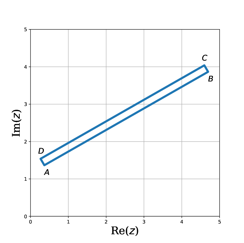
This fact allows us to adopt a subdivision-transformation-calculation scheme to ensure the algorithm stability. More specifically, the subdivision process is carried out in $z$-space. Noting that the subdivision scheme has been studied extensively by previous works delves67; kravanja98; kravanja99; kravanja99b, it is not necessary to go into details here. In this study, for simplicity, we search in rectangles to avoid redundancy during subdivision, with a generic example of the rectangle region searched shown in Fig. (1a). Once the rectangular vertexes, namely the points A, B, C and D in Fig. (1a), are given, the rectangle in $z$-space can be transformed to a slotted annulus right next to the unit circle in $\zeta$-space, as seen in Fig. (1b), via the transformation:

Here, the small positive parameter $\epsilon_{0}\ll 1$ is introduced to keep away from the branch cut of the complex logarithm in $\zeta$-space, $\alpha\in(-\pi,\pi]$ is the angle between the positive $\textrm{Re}(z)$-axis and the line $\overline{AB}$, and $z_{0}$ and $L$ are, respectively, the midpoint and length of $\overline{CD}$. Then, zeros and poles $(\zeta_{i},n_{i})$ are preliminarily calculated in $\zeta$-space by using the algorithm presented in Sec. (2), and the associated condition number of the Prony system is estimated by Eq. (24). If the condition number is larger than the preassigned value, one should suitably subdivide the region into smaller subregions in $z$-space, transform each subregion into $\zeta$-space, and calculate the corresponding zeros and poles. The subdivision-transformation-calculation process is repeated until the resulting condition number is acceptable.

Furthermore, it is also worthwhile noting that one feasibility of Eq. (24) lies in the identifying of primary factors influencing the stability of the system. Consistently with the fact that the total time taken is mainly set by the number of regions, it is possible and desirable to develop a more sophisticated subdivision scheme and, thus, to significantly improve the efficiency of algorithm. This topic will be pursued in future publications.

As the generalized eigenvalue problem can be solved in well-condition, the algorithm still suffers the inherent numerical error stemming from the contour integration in $\zeta$-space.

Since the numerical differentiation is time-consuming and error-prone, we perform an integration by parts in Eq.(4) and use the logarithmic derivative to avoid evaluating $f^{\prime}$. In this case, the main difficulty is the multivalueness of the complex logarithm. Thus, in order to identify the same branch of $\ln f$ numerically, we write

with

and ensure a continuous extended argument $\Theta$ by keeping track of the numerical calculated principal value $Arg(f)$ and selecting appropriate $m$s. Then Eq.(4) becomes

with $\zeta_{s}$ and $\zeta_{e}$ denoting the starting-point and end-point of the contour integration. Introducing the complex logarithm in this way provides several benefits. First, it avoids the evaluating of $f^{\prime}$. Second, since $[\zeta^{k}\ln f]_{\zeta_{s}}^{\zeta_{e}}/(2\pi i)$ is an integer, it can be computed accurately as with the Nyquist stability criterion. Third, the complex logarithm is more robust against the overflow and underflow issues.

Having obtained the zeros and poles, an important question arises as to how to estimate the error level. This can be addressed by the following theorem.

Theorem (4.1) provides a convenient way to estimate the order of absolute errors. Let $\zeta_{i}^{(0)}$ and $\zeta_{i}^{(1)}$ be the same eigenvalue calculated, respectively, from $\bar{\mathbf{H}}_{1,N}-\lambda\bar{\mathbf{H}}_{0,N}$ and $\bar{\mathbf{H}}_{1,N+1}-\lambda\bar{\mathbf{H}}_{0,N+1}$, then the numerical error can be simply estimated by

It should be emphasized that, due to the $N+1$ cofactors involved and $|a_{l}|\sim\mathcal{O}(1)$ near the unit cile, $\zeta_{i}^{(1)}$ is essentially a weighted average over the results of $N+1$ equivalent pencils.

To verify the strategies described in Secs. (3) and (4), we have implemented the algorithm to carry out illustrative examples. Specifically, the algorithm can be sketched as follows:

1. Step 1

   Set a critical condition number $\kappa^{2}_{c}$ and an error tolerance of the contour integration $\epsilon_{i}$;

2. Step 2

   Transform the rectangle region searched in $z$-space, say $\mathbb{D}$, to a slotted annulus in $\zeta$-space, with $\epsilon_{0}$ introduced to avoid the branch cut of the complex logarithm;

3. Step 3

   Construct Hankel matrices, determine their ranks and solve the pencil $\bar{\mathbf{H}}_{1,N}-\lambda\bar{\mathbf{H}}_{0,N}$;

4. Step 4

   Calculate the condition number $\kappa^{2}_{\infty}$ using Eq.(24),

   • •

     if $\kappa^{2}_{\infty}>\kappa^{2}_{c}$, subdivide $\mathbb{D}$ into smaller subregions $\mathbb{D}_{i}$, and go back to Step 2;

   • •

     otherwise, continue;

5. Step 5

   Solve the corrupted pencil $\bar{\mathbf{H}}_{1,N+1}-\lambda\bar{\mathbf{H}}_{0,N+1}$ for error estimate;

6. Step 6

   Multiplicities are obtained via the associated Vandermonde system, i.e., Eq.(4).

The following numerical examples serve as tests of the algorithm, and illuminate the potential applications to plasma physics. Multiplicities are recovered successfully in all cases.

References

- (1) H. Nyquist, Regeneration theory, Bell Syst. Tech., 11, 126 (1932).
- (2) L. M. Delves and J. N. Lyness, A numerical method for locating the zeros of an analytic function, Math. Comp., 21, 543 (1967).
- (3) L. F. Abd-Elall, L. M. Delves and J. K. Reid, A numerical method for locating the zeros and poles of a meromorphic function, in Numerical methods for nonlinear algebraic equations, (P. Rabinowitz, ed.), pp. 47-59, Gordon and Breach, London, (1970).
- (4) P. Kravanja, P. Cools and A. Haegemans, Computing zeros of analytic mappings: A logarithmic residue approach, BIT Numer. Math., 38, 583 (1998).
- (5) P. Kravanja, T. Sakurai and M. Van Barel, On locating clusters of zeros of analytic functions, BIT Numer. Math., 39, 646 (1999).
- (6) P. Kravanja and M. Van Barel, A derivative-free algorithm for computing zeros of analytic mappings, Computing, 63, 69 (1999).
- (7) F. B. Hildebrand, Introduction to numerical analysis (second edn), pp. 457-462, Dover, New York, (1987).
- (8) D. L. Boley, F. T. Luk and D. Vandevoorde, Vandermonde factorization of a Hankel matrix, in Scientific Computing, pp 27-39, Springer, Singapore, (1997).
- (9) G. H. Golub and C. F. Van Loan, Matrix computations (third edn), pp 405-419, Johns Hopkins University Press, Baltimore, (2013).
- (10) G. H. Golub and C. F. Van Loan, Matrix computations (4th edn), pp 87-93, Johns Hopkins University Press, Baltimore, (2013).
- (11) W. Gautschi, On inverses of Vandermonde and confluent Vandermonde matrices, Numer. Math., 4, 119 (1962).
- (12) T. Betcke, N. J. Higham, V. Mehrmann, C. Schroder and F. Tisseur, NLEVP: A collection of nonlinear eigenvalue problems, MIMS EPrint, (2011).
- (13) B. D. Fried and S. D. Conte, The plasma dispersion function, pp. 1-8, Academic Press, London and New York, (1961).
- (14) H. Chen and L. Chen, Gyrokinetic theory of low-frequency electromagnetic waves in finite- anisotropic plasmas, Phys. Plasmas, 28, 052103 (2021).
- (15) E. A. Frieman and L. Chen, Nonlinear gyrokinetic equations for low‐frequency electromagnetic waves in general plasma equilibria, Phys. Fluids, 25, 502 (1982).
- (16) L. Chen and A. Hasegawa, Kinetic theory of geomagnetic pulsations: 1. Internal excitations by energetic particles, J. Geophs. Res., 96, 1503 (1991).
- (17) A. J. Brizard and T. S. Hahm, Foundations of nonlinear gyrokinetic theory, Rev. Mod. Phys., 79, 421 (2007).
- (18) A. Hasegawa and L. Chen, Kinetic Process of Plasma Heating Due to Alfvén Wave Excitation, Phys. Rev. Lett., 35, 370 (1975).
- (19) A. Hasegawa and L. Chen, Kinetic processes in plasma heating by resonant mode conversion of Alfvén wave, Phys. Fluids, 19, 1924 (1976).