Optically detected flip-flops between different spin ensembles in diamond

A color center in diamond composed of a substitutional nitrogen and a vacancy in the crystal lattice (NV) Doherty et al. 2013 draws lately a considerable attention, particularly in the negatively charged state (NV^-). The NV^-electronic spin state can be polarized and read out with light. Dense ensembles of NV^-centers were demonstrated to be applicable for magnetometry Rondin et al. 2014, classical Dhomkar et al. 2016 and quantum Zhu et al. 2011; Kubo et al. 2011; Amsüss et al. 2011; Grezes et al. 2014 information storage, and recently, a maser implementation Breeze et al. 2018.

Dipolar coupling affecting a given NV^-in a diamond crystal is commonly dominated by other NV^-s, having either parallel or non-parallel lattice orientation, and by substitutional nitrogen (P1) defects, having a density typically higher by at least an order of magnitude. The interaction between the ensembles might be a quantum resource Bermudez et al. 2011 or a source of decoherence Bar-Gill et al. 2012.

Spontaneous, i.e. phonon assisted, spin flip-flops between ensembles (when one of the spins changes from high to low energy states, and the other changes in the opposite direction), were demonstrated before Bloembergen et al. 1959; Alfasi et al. 2019; Armstrong et al. 2010; Wang et al. 2014. In this work we demonstrate direct and unambiguous stimulated flip-flop interaction between the parallel and the non-parallel NV^-ensembles or the P1 ensemble. A higher order process involving five spins interaction is reported elsewhere Masis et al. 2019. In addition, we observe dipolar spin-spin interaction Waller 1932 at double the Larmor frequency inside a single NV^-ensemble parallel to the external magnetic field. The increased sensitivity of our setup is attributed to a combination of high NV^-density, low temperature and lock-in amplification.

In the context of sensing, our results may be described as optically detected electron-electron double resonance Dorio 2012 (ELDOR, also known as DEER). Unlike the traditional, microwave (MW) cavity based ELDOR, optical detection allows increased sensitivity, wide range of MW frequencies and higher spacial resolution. In the context of hyperpolarization Belthangady et al. 2013, our method is closely related to dynamic nuclear polarization Kamp et al. 2018a (DNP), where in the role of slow nuclear spins are the electronic spins of the P1, and in the role of fast electron spins are the optically polarized NV^-. Hyperpolarized P1 then might serve as a low noise spin bath for the NV^-, or as a target spin ensemble on its own right, e.g. for applications of P1 maser.

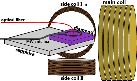
When hyperfine interaction is disregarded, the NV^-ground state spin triplet Hamiltonian becomes Ovartchaiyapong et al. 2014; MacQuarrie et al. 2013

where $D_{\mathrm{NV}}=2\pi\times 2.87~\mathrm{GHz}$ is the zero field splitting, $E_{\mathrm{NV}}\ll D_{\mathrm{NV}}$ is a strain-induced splitting, $\gamma_{\mathrm{e}}=2\pi\times 28.03~\mathrm{GHz}\mathrm{T}^{-1}$ is the electron spin gyromagnetic ratio, $\mathbf{B}$ is the applied magnetic field, $\mathbf{S}=S_{x}\mathbf{\hat{x}}+S_{y}\mathbf{\hat{y}}+S_{z}\mathbf{\hat{z}}$ is the spin $S=1$ angular momentum vector operator and $S_{\pm}=S_{x}\pm iS_{y}$. Under continuous laser excitation, NV^-is polarized to the spin state having magnetic quantum number $m_{\mathrm{S}}=0$, which has a slightly brighter photoluminescence (PL) Doherty et al. 2013. Introducing MW irradiation at frequency $\omega_{\mathrm{{LA}}}/2\pi$ resonant with $m_{\mathrm{S}}=0$ to $m_{\mathrm{S}}=\pm 1$ transition reduces the spin polarization and PL, allowing optical detection of the magnetic resonance (ODMR). We will use a nomenclature of $T_{v}^{i,j}$ to indicate a resonant transition in NV^-center parallel to vector $v\in\{\alpha,\beta,\gamma,\delta\}$ (see inset in Fig. 1) from state $i$ to state $j$, where $i,j\in\{-1,0,+1\}$. Both $i$ and $j$ states are eigenstates of the Hamiltonian $\mathcal{H}_{\mathrm{NV}}$ (1), where $i$ and $j$ indicate the magnetic quantum number $m_{\mathrm{S}}$ when $[\mathcal{H}_{\mathrm{NV}},S_{z}]=0$ (i.e. when the externally applied magnetic field $\mathbf{B}$ is parallel to the symmetry axis of the NV^-center, and strain-induced splitting is disregarded). A typical ODMR plot is shown in Fig. 2.

Our ODMR plots show not only the NV^-resonances, but also other defects. Among them - nitrogen 14 (nuclear spin 1) substitution defect (P1) in diamond Cook and Whiffen 1966; Loubser and van Wyk 1978, which has four locally stable configurations. In each configuration a static Jahn-Teller distortion Smith et al. 1959 occurs, and an unpaired electron is shared by the nitrogen atom and by one of the four neighboring carbon atoms, which are positioned along one of the lattice directions $\left\langle 111\right\rangle$ Takahashi et al. 2008; Hanson et al. 2006; Hanson et al. 2008; Wang et al. 2014; Broadway et al. 2016; Shim et al. 2013; Smeltzer et al. 2011; Shin et al. 2014; Clevenson et al. 2016; Schuster et al. 2010. The transition frequencies are calculated (see Figs. 2, 5 and 6) by numerically diagonalizing the P1 spin Hamiltonian $\mathcal{H}_{\mathrm{P}1}$ Cox et al. 1994; Alfasi et al. 2019 using the following parameters: nitrogen 14 nuclear gyromagnetic ratio $\gamma_{\mathrm{n}}=2\pi\times 3.0766\operatorname{MHz}$, nitrogen 14 quadrupole coupling $Q_{\mathrm{P}1}=-2\pi\times 3.97\operatorname{MHz}$, longitudinal hyperfine coupling $A_{\mathrm{P}1,\parallel}=2\pi\times 114\operatorname{MHz}$ and transverse hyperfine coupling $A_{\mathrm{P}1,\parallel}=2\pi\times 81.3\operatorname{MHz}$.

Type Ib HPHT single crystal $[110]$ grown diamond with $<200~\mathrm{ppm}$ nitrogen concentration (same as in Alfasi et al. 2019) was laser-cut, polished, irradiated with $2.8~\mathrm{MeV}$ electrons at a doze of $8\times 10^{18}~\mathrm{e/cm^{2}}$, annealed for $2~\mathrm{h}$ at $900~\mathrm{C}$ and boiled for $1~\mathrm{h}$ in equal mixture of Perchloric, Sulfuric and Fuming Nitric acids, resulting with a fluorescent-count measured NV^-concentration of $n_{\mathrm{S}}=3.25\times 10^{17}~\mathrm{cm^{-3}}$. The NV^-:P1 ratio is estimated from electron spin resonance (ESR) data to be $1:3$ (see Fig. 3) Alfasi et al. 2019. The diamond is oriented at room temperature to have the $\alpha([1\bar{1}\bar{1}])$ axis coinciding with the main coil axis and the (110) surface orthogonal to the 2nd coil. The diamond wafer is glued to a sapphire substrate carrying a $1.05~\mathrm{GHz}$ superconducting spiral resonator (see Fig. 1). The resonator is not used in this experiment. All measurements are performed at $3.5~\mathrm{K}$. Throughout the paper, the diamond misalignment is fit by azimuthal $\theta=2.86^{\circ}$ and polar $\phi=1.71^{\circ}$ angles with respect to the coordinate system defined by the axial directions of the 1st, 2nd and the main superconducting coils (see Fig. 1). A $637~\mathrm{nm}$ red laser is used to excite the NV centers at the NV^-zero-phonon line (ZPL), rather than the more commonly used $532~\mathrm{nm}$, in order to reduce sample heating. Despite the expected photoionization to the neutrally charged NV state, no trace of these defects was recorded in the ODMR scans. The returning PL light passes through a beam splitter and a $700~\mathrm{nm}$ long pass filter before measurement with a reverse-biased photo-diode (PD). MW loop antenna is connected directly to a synthesizer, $100\%$ amplitude modulated by a $151~\mathrm{Hz}$ sine wave. The PD signal is demodulated by a lock-in amplifier Anishchik and Ivanov 2017, and the resulting amplitude is recorded. In all the two dimensional scans the magnetic field is scanned first, slowly enough to avoid hysteresis.

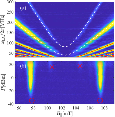
For NV^-aligned closely along the magnetic field direction (having a misalignment angle $|\psi|\ll 1~\mathrm{rad}$), a ground state levels anticrossing (GSLAC) between the states $m_{\mathrm{S}}=0$ and $m_{\mathrm{S}}=-1$ occurs at $D_{\mathrm{NV}}/\gamma_{\mathrm{e}}=102.4~\mathrm{mT}$. The resonance angular frequency $\omega_{\mathrm{{a}}}$ and the effective transverse drive amplitude $\omega_{\mathrm{{t}}}$ are given Masis et al. 2019; Masis by

where $\omega_{\mathrm{{a0}}}=\sqrt{2}D_{\mathrm{NV}}|\psi|$, $\omega_{\mathrm{{LA1}}}$ is the MW loop antenna drive amplitude, and the dimensionless detuning parameter $\eta$ is given by $\eta=(D_{\mathrm{NV}}-\gamma_{\mathrm{e}}B)/\omega_{\mathrm{{a0}}}$. The signal is recognizable in the ODMR scan as a hyperbola disappearing near the GSLAC, due to spin states mixing and subsequent inefficient MW depolarization required for the ODMR contrast.

Dipolar coupling gives rise to an absorption resonance at an angular frequency $2\omega_{\mathrm{{a}}}$ [second hyperbola, see Fig. 4(a)], due to spins flip-flip. Fractional hyperbolas at angular frequencies $\omega_{\mathrm{{a}}}/l$ for integer $l$ are attributed to multi-photon processes or higher harmonics in the excitation signal. The Bloch-Siegert shift corresponding to the $l$’th multi-photon processes is given by [see Eq.(6.378) of  Buks 2020]

where $\omega_{\mathrm{S}1}$ is longitudinal excitation amplitudes. The shift is too small to be resolved in our measurements, hence we conclude that $\omega_{\mathrm{{LA1}}}<1~\mathrm{MHz}$, and the ODMR linewidth is caused not by power broadening, but by increased NV^-transverse relaxation or by inhomogeneous broadening.

The ratio between the second and first hyperbolas strength at the effective magnetic field $B_{\mathrm{a}}=\omega_{\mathrm{{a}}}/\gamma_{\mathrm{e}}$ is given by Anderson 1962; Cheng 1961; Broer 1943; Daycock and Jones 1969

where, for disordered defects location, the azimuthally averaged local field is $\langle(\Delta B)^{2}\rangle_{av}=\pi\mu_{0}^{2}\hbar^{2}\gamma^{2}_{\mathrm{e}}S(S+1)\Sigma_{j}r_{ij}^{-6}$ and $r_{ij}$ is the distance between defects $i$ and $j$. For diluted diamond lattice $\Sigma_{j}r_{ij}^{-6}=r_{\mathrm{eff}}^{-6}$, where we calculate $r_{\mathrm{eff}}=0.907/\sqrt[3]{\rho_{\mathrm{NV}}}$ and $\rho_{\mathrm{NV}}=3.25/4\times 10^{17}~\mathrm{cm}^{-3}$ is the density of NV^-parallel to one of the crystallographic vectors. A quantitative comparison of first and second hyperbolas visibility is given in Fig. 4(b), and a good agreement to optically determined NV concentration is found.

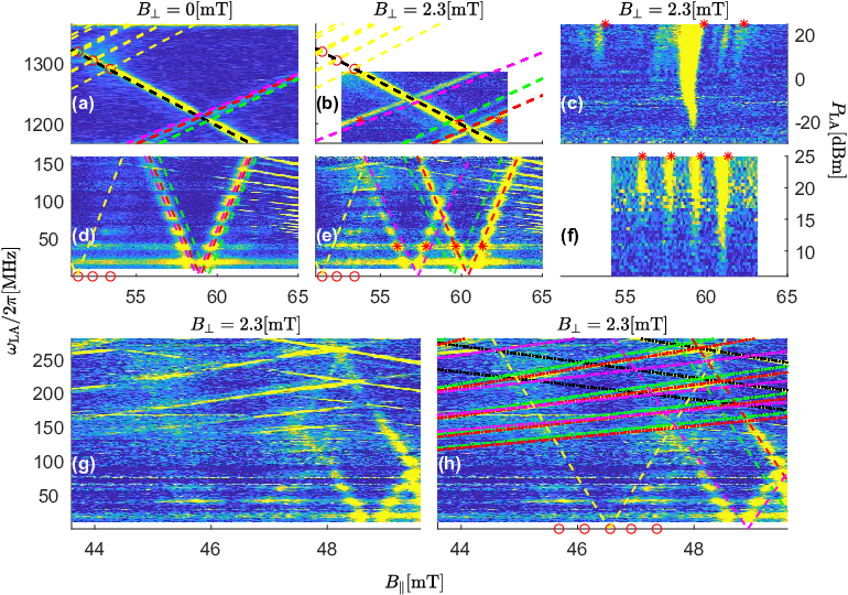
We observe dipolar spin flip-flop lines between ensembles of different NV^-orientations, specifically between the $T^{-1,0}_{\alpha}$ transition of the NV^-parallel to the main coil magnetic field and $T^{-1,+1}_{\beta,\gamma,\delta}$ transitions of the remaining three NV^-orientations [see Fig. 5(d)]. The signal visibility of $T^{-1,+1}_{\beta,\gamma,\delta}$ is low as compared to $T^{-1,0}_{\alpha}$ [see Fig. 5(c)], and therefore the flip-flop ODMR signal is attributed mostly to the latter. Applying magnetic field $B_{\perp}$ in the $\left[110\right]$ direction by increasing the current in the 2nd coil lifts the geometric degeneracy of the three non-parallel NV^-vectors [see Fig. 5(b)]. The visibility of $T^{-1,+1}_{\beta}$ is much smaller than the visibility of $T^{-1,+1}_{\gamma,\delta}$, probably due to the orientation with respect to the MW antenna, and the corresponding flip-flop signal was not detected. The relative strength of the flip-flop signal [Fig. 5(f)] is comparable (Abragam and Goldman 1982, p. 357) to the same spin flip-flip case [Fig. 4 (b)] (i.e. both signals become detectable at an input power of $10~\mathrm{dBm}$).

In addition, faint diagonal lines circa $53~\mathrm{mT}$ are attributed to a spin-flip process between the parallel NV^-and an additional electronic spin-$1/2$ ensemble [Fig. 5(g)]. A suitable candidate is the P1 ensemble, though the signal strength does not allow reliable fit of the hyperfine lines. The expected P1 concentration is comparable to NV^-, yet the NV^--P1 flip-flop is hardly registered.

A possible explanation is an efficient hyper-polarization of the P1 centers as compared to the non-parallel NV^-centers, leading to a lower flip-flop probability. The reduced non-parallel NV^-hyperpolarization may in turn be explained by spin flips during optical excitation-relaxation cycles or during photoionization and electron re-trapping. Yet a different explanation could be a photo-ionisation of the substitutional nitrogen, effectively reducing the concentration of the paramagnetic P1 centers Doherty et al. 2016; Lawson et al. 1998. However, the data of Fig. 6 suggests that the P1 concentration is significant enough to alter the NV^-ODMR even when the P1 frequency is detuned far from the NV^-resonance.

In low frequency region all observed ODMR lines are modulated with a pattern having a characteristic beating frequency given by $f_{\mathrm{a}}=20.4~\mathrm{MHz}$ (Fig. 7). The beating can be attributed to strain coupling to bulk acoustic standing waves in the diamond wafer Golter et al. 2016; Nakamura et al. 2003; Ovartchaiyapong et al. 2012. However, the speed of sound of $2f_{\mathrm{a}}t=20.4~\mathrm{Km/s}$, which is derived from the measured beating frequency $f_{\mathrm{a}}$ and the thickness of the diamond wafer $t=0.5~\mathrm{mm}$, is about 13% higher than the values reported in  McSkimin and Bond 1957; McSkimin and Andreatch Jr 1972; Nakamura et al. 2003.

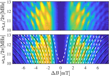
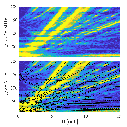
The ODMR data shown in Fig. 8 for the frequency range of 10-13 MHz exhibits a complex modulation pattern. Three nuclear spins have been considered to explain the data. The nuclear spin 1 of nitrogen 14 of P1 defects is ruled out since its transition frequency is not expected to significantly change near NV^-GSLAC, whereas the data exhibits modulation pattern of arcs symmetric around $102~\mathrm{mT}$. The spin 1 of nitrogen 14 of the NV- defects is ruled out since its hyperfine coupling is too weak. First shell 13C has both sufficiently strong hyperfine coupling and its transition frequency strongly varies near $102~\mathrm{mT}$, however the high symmetry of the data is not compatible with 13C energy levels. Perplexedly, the arcs in the figure can be fitted by a single curve, stretched along the magnetic field axis by an integer factor (see caption of Fig. 8).

We report of optical detection of driven spin flip-flop, yet many questions remain unanswered with regard to the strength of perceived signal. For bath-control applications, of utter importance is the poor visibility of NV^--P1 flip-flop line, which suggests high efficiency of P1 optical DNP process. With regards to NV^--NV^-flip flops, the $\beta$ direction stands out, with both poor visibility of $T^{-1,+1}_{\beta}$ transition and the lack of detectable flip-flop with $T^{-1,0}_{\alpha}$. In addition, no flip-flip lines at $2T^{-1,+1}_{\beta,\gamma,\delta}$ were detected. Further studies altering the relative orientations of the diamond, bias magnetic field and MW excitation may provide further insight regarding the strength of the various flip-flop lines, particularly in relation to the well understood flip-flip line strength. The strength of the flip-flop lines may be measured to optimize the efficiency of applied hyperpolarization protocols - i.e., after efficient hyperpolarization there are more aligned spins and less misaligned, hence flip-flop line is suppressed and the flip-flip line is emphasized.

We thank Aharon Blank, Amit Finkler and Nir Bar Gill for fruitful discussions. This work was supported by the Israel science foundation, any by the Israel ministry of science.

References

- Doherty et al. (2013) M. W. Doherty, N. B. Manson, P. Delaney, F. Jelezko, J. Wrachtrup, and L. C. Hollenberg, Physics Reports 528, 1 (2013).
- Rondin et al. (2014) L. Rondin, J. Tetienne, T. Hingant, J. Roch, P. Maletinsky, and V. Jacques, Reports on Progress in Physics 77, 056503 (2014).
- Dhomkar et al. (2016) S. Dhomkar, J. Henshaw, H. Jayakumar, and C. A. Meriles, Science advances 2, e1600911 (2016).
- Zhu et al. (2011) X. Zhu, S. Saito, A. Kemp, K. Kakuyanagi, S.-i. Karimoto, H. Nakano, W. J. Munro, Y. Tokura, M. S. Everitt, K. Nemoto, et al., Nature 478, 221 (2011).
- Kubo et al. (2011) Y. Kubo, C. Grezes, A. Dewes, T. Umeda, J. Isoya, H. Sumiya, N. Morishita, H. Abe, S. Onoda, T. Ohshima, et al., Physical review letters 107, 220501 (2011).
- Amsüss et al. (2011) R. Amsüss, C. Koller, T. Nöbauer, S. Putz, S. Rotter, K. Sandner, S. Schneider, M. Schramböck, G. Steinhauser, H. Ritsch, et al., Phys. Rev. Lett. 107, 060502 (2011), URL http://link.aps.org/doi/10.1103/PhysRevLett.107.060502.
- Grezes et al. (2014) C. Grezes, B. Julsgaard, Y. Kubo, M. Stern, T. Umeda, J. Isoya, H. Sumiya, H. Abe, S. Onoda, T. Ohshima, et al., Physical Review X 4, 021049 (2014).
- Breeze et al. (2018) J. D. Breeze, E. Salvadori, J. Sathian, N. M. Alford, and C. W. Kay, Nature 555, 493 (2018).
- Bermudez et al. (2011) A. Bermudez, F. Jelezko, M. Plenio, and A. Retzker, Physical review letters 107, 150503 (2011).
- Bar-Gill et al. (2012) N. Bar-Gill, L. M. Pham, C. Belthangady, D. Le Sage, P. Cappellaro, J. Maze, M. D. Lukin, A. Yacoby, and R. Walsworth, Nature communications 3, 1 (2012).
- Bloembergen et al. (1959) N. Bloembergen, S. Shapiro, P. Pershan, and J. Artman, Physical Review 114, 445 (1959).
- Alfasi et al. (2019) N. Alfasi, S. Masis, O. Shtempluck, and E. Buks, Phys. Rev. B 99, 214111 (2019).
- Armstrong et al. (2010) S. Armstrong, L. J. Rogers, R. L. McMurtrie, and N. B. Manson, Physics Procedia 3, 1569 (2010).
- Wang et al. (2014) H.-J. Wang, C. S. Shin, S. J. Seltzer, C. E. Avalos, A. Pines, and V. S. Bajaj, Nature communications 5, 4135 (2014).
- Masis et al. (2019) S. Masis, N. Alfasi, R. Levi, O. Shtempluck, and E. Buks, Phys. Rev. A 100, 013852 (2019).
- Waller (1932) I. Waller, Zeitschrift für Physik 79, 370 (1932).
- Dorio (2012) M. M. Dorio, Multiple electron resonance spectroscopy (Springer Science & Business Media, 2012).
- Belthangady et al. (2013) C. Belthangady, N. Bar-Gill, L. M. Pham, K. Arai, D. Le Sage, P. Cappellaro, and R. L. Walsworth, Physical review letters 110, 157601 (2013).
- Kamp et al. (2018a) E. Kamp, B. Carvajal, and N. Samarth, Physical Review B 97, 045204 (2018a).
- Felton et al. (2009) S. Felton, A. Edmonds, M. Newton, P. Martineau, D. Fisher, D. Twitchen, and J. Baker, Physical Review B 79, 075203 (2009).
- Mizuochi et al. (2009) N. Mizuochi, P. Neumann, F. Rempp, J. Beck, V. Jacques, P. Siyushev, K. Nakamura, D. Twitchen, H. Watanabe, S. Yamasaki, et al., Physical review B 80, 041201 (2009).
- Simanovskaia et al. (2013) M. Simanovskaia, K. Jensen, A. Jarmola, K. Aulenbacher, N. Manson, and D. Budker, Physical Review B 87, 224106 (2013).
- Kamp et al. (2018b) E. Kamp, B. Carvajal, and N. Samarth, Physical Review B 97, 045204 (2018b).
- Loubser and van Wyk (1978) J. Loubser and J. van Wyk, Reports on Progress in Physics 41, 1201 (1978).
- Alfasi et al. (2018) N. Alfasi, S. Masis, R. Winik, D. Farfurnik, O. Shtempluck, N. Bar-Gill, and E. Buks, Physical Review A 97, 063808 (2018).
- Ovartchaiyapong et al. (2014) P. Ovartchaiyapong, K. W. Lee, B. A. Myers, and A. C. B. Jayich, arXiv:1403.4173 (2014).
- MacQuarrie et al. (2013) E. MacQuarrie, T. Gosavi, N. Jungwirth, S. Bhave, and G. Fuchs, Physical review letters 111, 227602 (2013).
- Cook and Whiffen (1966) R. Cook and D. Whiffen, Proceedings of the Royal Society of London A: Mathematical, Physical and Engineering Sciences 295, 99 (1966).
- Smith et al. (1959) W. Smith, P. Sorokin, I. Gelles, and G. Lasher, Physical Review 115, 1546 (1959).
- Takahashi et al. (2008) S. Takahashi, R. Hanson, J. van Tol, M. S. Sherwin, and D. D. Awschalom, Physical review letters 101, 047601 (2008).
- Hanson et al. (2006) R. Hanson, F. Mendoza, R. Epstein, and D. Awschalom, Physical review letters 97, 087601 (2006).
- Hanson et al. (2008) R. Hanson, V. Dobrovitski, A. Feiguin, O. Gywat, and D. Awschalom, Science 320, 352 (2008).
- Broadway et al. (2016) D. A. Broadway, J. D. Wood, L. T. Hall, A. Stacey, M. Markham, D. A. Simpson, J.-P. Tetienne, and L. C. Hollenberg, arXiv:1607.04006 (2016).
- Shim et al. (2013) J. Shim, B. Nowak, I. Niemeyer, J. Zhang, F. Brandao, and D. Suter, arXiv:1307.0257 (2013).
- Smeltzer et al. (2011) B. Smeltzer, L. Childress, and A. Gali, New Journal of Physics 13, 025021 (2011).
- Shin et al. (2014) C. S. Shin, M. C. Butler, H.-J. Wang, C. E. Avalos, S. J. Seltzer, R.-B. Liu, A. Pines, and V. S. Bajaj, Physical Review B 89, 205202 (2014).
- Clevenson et al. (2016) H. Clevenson, E. H. Chen, F. Dolde, C. Teale, D. Englund, and D. Braje, Phys. Rev. A 94, 021401 (2016).
- Schuster et al. (2010) D. Schuster, A. Sears, E. Ginossar, L. DiCarlo, L. Frunzio, J. Morton, H. Wu, G. Briggs, B. Buckley, D. Awschalom, et al., Physical review letters 105, 140501 (2010).
- Cox et al. (1994) A. Cox, M. Newton, and J. Baker, Journal of Physics: Condensed Matter 6, 551 (1994).
- Anishchik and Ivanov (2017) S. V. Anishchik and K. L. Ivanov, Physical Review B 96, 115142 (2017).
- (41) S. Masis, Dipolar interactions between dense spinensembles in diamond.
- Buks (2020) E. Buks, Quantum mechanics - Lecture Notes (http://buks.net.technion.ac.il/teaching/, 2020), URL http://buks.net.technion.ac.il/teaching/.
- Anderson (1962) A. Anderson, Physical Review 125, 1517 (1962).
- Cheng (1961) H. Cheng, Physical Review 124, 1359 (1961).
- Broer (1943) L. Broer, Physica 10, 801 (1943).
- Daycock and Jones (1969) J. Daycock and G. P. Jones, Journal of Physics C: Solid State Physics 2, 998 (1969).
- Abragam and Goldman (1982) A. Abragam and M. Goldman (1982).
- Doherty et al. (2016) M. Doherty, C. A. Meriles, A. Alkauskas, H. Fedder, M. J. Sellars, and N. B. Manson, Physical Review X 6, 041035 (2016).
- Lawson et al. (1998) S. C. Lawson, D. Fisher, D. C. Hunt, and M. E. Newton, Journal of Physics: Condensed Matter 10, 6171 (1998).
- Golter et al. (2016) D. A. Golter, T. Oo, M. Amezcua, K. A. Stewart, and H. Wang, Physical review letters 116, 143602 (2016).
- Nakamura et al. (2003) N. Nakamura, H. Ogi, T. Ichitsubo, M. Hirao, N. Tatsumi, T. Imai, and H. Nakahata, Journal of applied physics 94, 6405 (2003).
- Ovartchaiyapong et al. (2012) P. Ovartchaiyapong, L. Pascal, B. Myers, P. Lauria, and A. B. Jayich, Applied Physics Letters 101, 163505 (2012).
- McSkimin and Bond (1957) H. McSkimin and W. Bond, Physical Review 105, 116 (1957).
- McSkimin and Andreatch Jr (1972) H. McSkimin and P. Andreatch Jr, Journal of Applied Physics 43, 2944 (1972).