We will now explain how the cost in (4) is replaced by a finite sum via a Monte Carlo approximation. Assume for the moment that we can draw $M>0$ samples from the distribution $p(x_{t},\theta,\mathbf{w}_{t}|y_{1:t},u_{1:t})$ such that

where the superscript $i$ will be used to indicate that this was the $i^{\text{th}}$ such sample out of $M$. Then via the Law of Large Numbers, we arrive at the following Monte Carlo approximation

The primary benefit is that this is now a finite sum and a deterministic function of $\mathbf{u}_{t}$ since the samples are fixed. Under mild regularity conditions, the approximation converges almost surely to the desired expectation as $M\to\infty$ [26]. In practice we are forced to choose a finite $M$ and deal with any consequences, which will be highly problem dependent.

Returning to the assumption that we are able to draw samples from the desired conditional distribution, this is by no means trivial and significant research attention has been directed towards solving it (see e.g. [21, 11, 1]). One of the most successful approaches to producing these samples is to construct a Markov chain whose stationary distribution coincides with the desired target distribution $p(x_{t},\theta,\mathbf{w}_{t}|y_{1:t},u_{1:t})$. Together, the use of a Markov chain with the Monte Carlo approximation leads to the MCMC approaches.

In this paper, we suggest the use of HMC, which uses a Hamiltonian system to construct such a Markov chain. Alternates include Particle Markov chain Monte Carlo [1] and Particle Gibbs with ancestor sampling [17]. While the intricate details of HMC are beyond the scope of this paper, in essence, the HMC approach is a version of the Metropolis-Hastings algorithm [2, 20], where the essential steps in each iteration are described in Algorithm 1. A discussion of the methods for determining the integration time $L$ and the mass matrix $\Sigma_{k}$ as well as the optimal target acceptance rate are beyond the scope of this paper and the interested reader is referred to [2]. Further, the required derivatives are typically computed using automatic differentiation.

The benefit of using HMC is that it is very efficient and the algorithm progresses with high acceptance ratio¹¹ 1 This arises since Hamiltonian systems are energy preserving and hence, theoretically, $H(\eta_{L},\rho_{L})=H(\eta_{0},\rho_{0})$ and the acceptance ratio will be one. and with low correlation in the chain [20]. For the simulations provided in this paper, we used the stan software package [25] with full details provided in the available github repository²² 2 https://github.com/jnh277/data_to_mpc. Further details of the HMC method for the current context are provided in [11].

The chance constraint can be converted into an expectation using the standard identity that

In the above, $\mathbb{I}(\cdot)$ is the indicator function that is one if the argument is true and zero otherwise. We can reuse the HMC method described above to also approximate this expectation using a finite sum via

where the samples $x_{t}^{i},\theta^{i},\mathbf{w}_{t}^{i}$ are reused from the cost approximation.

Unfortunately, the indicator function is discontinuous and this would result in a mixed-integer nonlinear programming problem, which is typically more challenging to solve. To avoid this, the indicator function is instead replaced by the logistic function

which coincides with the indicator function in the limit as $\gamma\to 0$. The probability of satisfying the constraint can therefore be approximated as

Let us now combine the above approximations and formulate a tractable optimisation problem, which is amenable to standard approaches. In addition to searching over the input sequence $\mathbf{u}_{t}$, we will also treat $\epsilon$ as a slack variable, where the aim is to reduce $\epsilon$ towards some user defined lower bound $\delta\geq 0$, but with the possibility that $\epsilon>\delta$ in order that the constraints form a non-empty feasible set.

Towards this, in what follows it will be convenient to define a new variable $\mathbf{z}_{t}$ as

and the $j^{\text{th}}$ element of a new function $g^{M}\in\mathbb{R}^{n_{cx}}$ as

Here, we have dropped the explicit reliance on $x_{t}^{i},\theta^{i}$ and $\mathbf{w}_{t}^{i}$ in order to reduce notation overhead. The optimisation problem can then be stated as

In the above, $\eta>0$ is a user-defined weighting term and $\epsilon_{0}\leq 0$ is used to offset the penalty on this slack variable.

The basic approach is to solve a sequence of these problems as $\gamma\to 0$, thus recovering the indicator function constraints in the limit. On the one hand, this is a nonlinear (and non-convex) programming problem with inequality constraints, and it is possible to employ standard software for solving this problem. On the other hand, it is not essential to obtain high precision solutions for each $\gamma$ value, since small changes in $\gamma$ are likely to produce small changes in the solution.

Motivated by this, we derive an interior-point method (based on the log-barrier approach) that is amenable to solving a sequence of problems as $\gamma\to 0$ (see e.g. [7, 30]). To this end, the log-barrier method proceeds by first amending the cost with a log-barrier for each inequality constraint (where the logarithm of a vector is to be interpreted element-wise)

In the above, $\mu>0$ is a barrier weighting term, and importantly, in the limit as $\mu\to 0$, the solution to

coincides with the solution to (14). The main benefit of this approach is that problem (16) is directly amenable to second-order unconstrained optimisation methods, such as Newton’s method. Note, this requires some care in ensuring that iterates remain in the feasible region of the log-barrier terms, which is straighforwardly handled, for example, by a modified line search procedure.

With this as background, the approach detailed in Algorithm 2 proceeds by solving the sequence of problems (16) where the barrier weighting $\mu$ and the sigmoid function parameter $\gamma$ are gradually reduced to zero.

In Algorithm 3 we summarise the resulting solution, which is demonstrated in Section IV.

First, the proposed approach is applied to a non-control affine first-order system to demonstrate the dual accomplishment of learning and control. Additionally, it highlights how the full probabilistic information about the states and parameters informs the control actions. Let us consider

where $\mathcal{T}(\nu,0,r^{2})$ is a Student’s T distribution with $\nu$ degrees of freedom and scale $r$. For this example, $a=0.9$, $b=0.2$, $r=0.05$, $\nu=4$, and $q=0.05$, the constraints $P(0\leq\mathbf{x}_{t}\leq 1.2)\geq 0.95$ are considered, and a set point of $x^{*}=1.0$ is chosen.

The system was simulated for $T=50$ discrete time steps. At each time step, Algorithm 3 was used to sample from the conditional distribution $p(x_{t},\theta|y_{1:t},u_{1:t},\nu)$ where $\theta=\{a,b,q,r\}$ in this case — with target and achieved acceptance rates of $80\%$ and $79\%$ — and to calculate the next control action $u_{t}$ using a horizon of $N=10$. Note that given a sample $q^{i}$ we can easily sample $\mathbf{w}_{t}^{i}$. The computation time per iteration was in the order of $4\text{\,}\mathrm{s}$.

Figure 1 shows the simulated and estimated state along with the control input and Figure 2 shows the parameter estimates at each time step. Relatively uninformative priors were placed on the initial state and on the parameters. As such, we can see that the estimates of the parameters and state become more certain as the amount of data $\{y_{1:t},u_{1:t}\}$ increases. Consequently, the control action becomes more aggressive and the state is driven closer whilst still satisfying the chance state constraint.

Additionally, examples of the predicted future states, $\mathbf{x}_{t}$, and optimised control actions over the horizon, $\mathbf{u}_{t}$, are provided in Figure 3. A trade-off exists between achieving the set point and satisfying the constraint with the desired probability. As a consequence, we can observe that the uncertainty on $\mathbf{x}_{t}$ grows the further into the future the prediction is and as a consequence the forecast control actions become more conservative in order to ensure the desired $95\%$ state constraint satisfaction at these future time steps.

The proposed method is now applied to a simulated rotational inverted pendulum, or Furata pendulum [8]. For the purpose of simulation the parameter values specified for the QUANSER^© QUBE-Servo 2 Rotary inverted pendulum in [10] are used.

Let the state vector used to model the Furata pendulum be $x=\begin{bmatrix}\vartheta&\alpha&\dot{\vartheta}&\dot{\alpha}\end{bmatrix}^{\mathsf{T}}$, where $\vartheta$ and $\alpha$ are the base arm and pendulum angles respectively, and the controllable input to the system be the motor voltage $V_{m}$. Then, the continuous time dynamics are given by

where $m_{p}$ is the pendulum mass, $L_{r}$, $L_{p}$ and the rod and pendulum lengths, $J_{r}$, $J_{p}$ are the rod and pendulum inertias, $R_{m}$ and $k_{m}$ are the motor resistance and constant, $D_{p}$ is the pendulum damping constant, and $D_{r}(\dot{\vartheta})$ is the arm damping function. Since a perfect damping model is unlikely, $D_{r}(\dot{\vartheta})=D_{r0}\text{sign}(\dot{\vartheta})+D_{r1}\dot{\vartheta}+D_{r2}\dot{\vartheta}^{2}$ was used for simulation and $D_{r}(\dot{\vartheta})=D_{r1}\dot{\vartheta}$ for estimation and control.

The process model used for simulation, estimation and control consists of a 4^th order Runge-Kutta discretisation of these continuous time dynamics over a $25$ms sampling time, subsequently disturbed by noise $w_{t}$. The input voltage from $t$ to $t+1$ is given by a zero-order hold of the control $u_{t}$.

Measurements are from encoders on the arm and pendulum angle and current measurements from the motor. The resulting measurement model is $y_{t}=\begin{bmatrix}\vartheta&\alpha&\frac{V_{m}-k_{m}\dot{\vartheta}}{R_{m}}\end{bmatrix}+e_{t}$. It is assumed that the elements of the process and measurement noise are all independent: $w_{t}\sim\mathcal{N}(0,\Sigma_{w})$ and $e_{t}\sim\mathcal{N}(0,\Sigma_{e})$, i.e. $\Sigma_{w}=\text{diag}([$3\text{\times}{10}^{-4}$,$1\text{\times}{10}^{-4}$,$0.013$,$0.013$])^{2}$ and $\Sigma_{e}=\text{diag}([$1.1\text{\times}{10}^{-3}$,$1\text{\times}{10}^{-3}$,$0.175$])^{2}$. $u_{t}$ is constrained to $[-18,18]$, $\vartheta$ is constrained to $\pm 270^{\circ}$ with $95\%$ probability, and the state cost $\vartheta^{2}+900(\cos(\alpha)-1)^{2}+$1\text{\times}{10}^{-10}$\dot{\vartheta}^{2}+$1\text{\times}{10}^{-10}$\dot{\alpha}$ is used.

The system was simulated for $T=50$ discrete time steps. At each time step Algorithm 3 samples from the joint conditional distribution of the state $x_{t}$ and the parameters, $\theta=\{J_{r},J_{p},K_{m},R_{m},D_{p},D_{r},\Sigma_{w},\Sigma_{e}\}$, given by $p(x_{t},\theta|y_{1:t})$ — with target and achieved acceptance rates of $85\%$ and $83\%$ — and calculate the control $u_{t+1}$ with a horizon of $N=25$. The computation time per iteration was in the order of $200\text{\,}\mathrm{s}$.

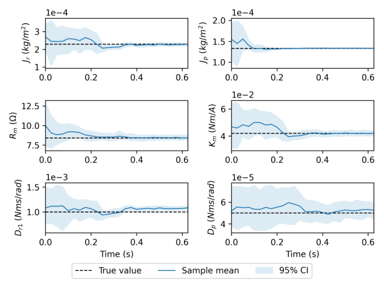
Figure 4 shows the true and estimated arm and pendulum angles as well as the control action and the total energy of the pendulum. Figure 5 shows the model parameter estimates at each discrete time step. These results show that the proposed method is capable of updating the state and parameter estimates as more data becomes available and using the full probabilistic information to determine the control in a nonlinear setting. An animation illustrating these results is available at https://youtu.be/E3_rUWejXEc.

References

- [1] C. Andrieu, A. Doucet, and R. Holenstein. Particle Markov chain Monte Carlo methods. Journal of the Royal Statistical Society: Series B (Statistical Methodology), 72(3):269–342, 2010.
- [2] M. Betancourt. A conceptual introduction to Hamiltonian Monte Carlo. Pre-print, 2017. arXiv:1701.02434.
- [3] A. Carron, E. Arcari, M. Wermelinger, L. Hewing, M. Hutter, and M. N. Zeilinger. Data-driven model predictive control for trajectory tracking with a robotic arm. IEEE Robotics and Automation Letters, 4(4):3758–3765, 2019.
- [4] J. Dahlin. Sequential Monte Carlo for inference in nonlinear state space models. Licentiate’s thesis no. 1652, Linköping University, May 2014.
- [5] A. A. Feldbaum. Dual control theory, part i. Avtomatika i Telemekhanika, 21(9):1240–1249, 1960.
- [6] M. Ferizbegovic, J. Umenberger, H. Hjalmarsson, and T. B. Schön. Learning robust LQ-controllers using application oriented exploration. IEEE Control System Letters, 4(1):19–24, 2020.
- [7] A. V. Fiacco and G. P. McCormick. Nonlinear programming: sequential unconstrained minimization techniques. SIAM, 1990.
- [8] K. Furuta, M. Yamakita, and S. Kobayashi. Swing-up control of inverted pendulum using pseudo-state feedback. Proceedings of the Institution of Mechanical Engineers, Part I: Journal of Systems and Control Engineering, 206(4):263–269, 1992.
- [9] N. Galioto and A. A. Gorodetsky. Bayesian system id: optimal management of parameter, model, and measurement uncertainty. Nonlinear Dynamics, 102(1):241–267, 2020.
- [10] Rotary Inverted Pendulum User Guides. Laboratories. Quanser Inc, 2003.
- [11] J. Hendriks, A. Wills, B. Ninness, and J. Dahlin. Practical Bayesian system identification using hamiltonian Monte Carlo. Technical report, arXiv:2011.04117, 2020.
- [12] Z. Hou and Z. Wang. From model-based control to data-driven control: Survey, classification and perspective. Information Sciences, 235:3–35, 2013.
- [13] A. Iannelli and R. S. Smith. A multiobjective LQR synthesis approach to dual control for uncertain plants. IEEE Control Systems Letters, 4(4):952–957, 2020.
- [14] M. Khalil, A. Sarkar, S. Adhikari, and D. Poirel. The estimation of time-invariant parameters of noisy nonlinear oscillatory systems. Journal of Sound and Vibration, 344:81–100, 2015.
- [15] P. Li, H. Arellano-Garcia, and G. Wozny. Chance constrained programming approach to process optimization under uncertainty. Computers & chemical engineering, 32(1-2):25–45, 2008.
- [16] Yingzhao Lian, Renzi Wang, and Colin N Jones. Koopman based data-driven predictive control. arXiv preprint arXiv:2102.05122, 2021.
- [17] F. Lindsten, M. I. Jordan, and T. B. Schön. Particle Gibbs with ancestor sampling. Journal of Machine Learning Research (JMLR), 15:2145–2184, June 2014.
- [18] N. Matni, A. Proutiere, A. Rantzer, and S. Tu. From self-tuning regulators to reinforcement learning and back again. In IEEE 58th Conference on Decision and Control (CDC), pages 3724–3740, 2019.
- [19] A. Mesbah. Stochastic model predictive control with active uncertainty learning: a survey on dual control. Annual Reviews in Control, 45:107–117, 2018.
- [20] R. M. Neal. MCMC using Hamiltonian dynamics. In S. Brooks, A. Gelman, G. Jones, and X-L. Meng, editors, Handbook of Markov Chain Monte Carlo. Chapman & Hall/CRC Press, 2010.
- [21] B. Ninness. Strong laws of large numbers under weak assumptions with application. IEEE Transactions on Automatic Control, 45(11):2117–2122, 2000.
- [22] S. Peng. Chance constrained problem and its applications. PhD thesis, Université Paris Saclay (COmUE); Xi’an Jiaotong University, 2019.
- [23] V. Peterka. Bayesian system identification. Automatica, 17(1):41–53, 1981.
- [24] B. Recht. A tour of reinforcement learning: The view from continuous control. Annual Review of Control, Robotics, and Autonomous Systems, 2(253–279), 2019.
- [25] Stan Development Team. Stan: A C++ library for probability and sampling, version 2.14.0, 2017.
- [26] Luke Tierney. Markov chains for exploring posterior distributions. the Annals of Statistics, pages 1701–1728, 1994.
- [27] J. Umenberger, M. Ferizbegovic, T. B. Schön, and H. Hjalmarsson. Robust exploration in linear quadratic reinforcement learning. In Neural Information Processing Systems 32 (NeurIPS), 2019.
- [28] J. Venkatasubramanian, J. Köhler, J. Berberich, and F. Allgöwer. Robust dual control based on gain scheduling. In 59th IEEE Conference on Decision and Control (CDC), pages 2270–2277, 2020.
- [29] K. P. Wabersich and M. Zeilinger. Bayesian model predictive control: Efficient model exploration and regret bounds using posterior sampling. In Learning for Dynamics and Control (L4DC), pages 455–464, 2020.
- [30] A. G. Wills and W. P. Heath. Barrier function based model predictive control. Automatica, 40(8):1415–1422, 2004.
- [31] L. Yingzhao and C. Jones. On gaussian process based koopman operator. Technical report, 2020.