Estimation of parameters of the Gumbel type-II distribution under AT-II PHCS with an application of Covid- data
Abstract
In this paper, we investigate the classical and Bayesian estimation of unknown parameters of the Gumbel type-II distribution based on adaptive type-II progressive hybrid censored sample (AT-II PHCS). The maximum likelihood estimates (MLEs) and maximum product spacing estimates (MPSEs) are developed and computed numerically using Newton-Raphson method. Bayesian approaches are employed to estimate parameters under symmetric and asymmetric loss functions. Bayesian estimates are not in explicit forms. Thus, Bayesian estimates are obtained by using Markov chain Monte Carlo (MCMC) method along with the Metropolis-Hastings (MH) algorithm. Based on the normality property of MLEs the asymptotic confidence intervals are constructed. Also, bootstrap intervals and highest posterior density (HPD) credible intervals are constructed. Further a Monte Carlo simulation study is carried out. Finally, the data set based on the death rate due to Covid-19 in India is analyzed for illustration of the purpose.
Keywords : Adaptive type-II progressive hybrid censoring; Maximum product spacing estimation; Markov chain Monte Carlo; Highest posterior density credible interval; Coverage probability; Covid-19 data set.
2010 Mathematics Subject Classification: 62N02; 62F10; 62F15
1 Introduction
In recent times, life testing experiments and reliability studies have achieved more acceptance. In such experiments, various situations appear where experimental units are eliminated before the time of failure. In these cases, the investigator may not have full information about the failure times of the whole experimental unit. Such kind of data collected from all these experiments are called censored data. It is worth mentioning that the censoring was introduced in practice to save time and reduce the number of failed units in a life-testing experiment.
Censoring can be done with respect to a prefixed time or prefixed number of failures or sometimes a combination of both prefixed time and number of failures. Depending upon these criteria, there are different types of censoring schemes. Let us consider a life testing experiment with number of experimental units and denotes the time of -th failure of the experimental units, where . Let be a pre-specified time. If all the experiments fail before that pre-specified time , it is known as a type-I censoring scheme. In the case of the type-II censoring scheme, the experiment will terminate after -th number of failures observed, where .
Both type-I and type-II censoring schemes have some disadvantages. In the case of type-I censoring, the number of failures may be zero, and in the case of type-II censoring, experimental time may be very large.
For further information about these schemes, we refer to Lawless 2011, Sirvanci and Yang 1984 and Balakrishnan and Chan 1992.
Epstein 1954 introduced a censoring scheme which is a mixture of type-I and type-II censoring schemes, known as the type-I hybrid censoring scheme. In this scheme, the experiment is terminated at time , where denotes the -th failure and is pre-specified time. Childs et al. 2003 proposed type-II hybrid censoring scheme where experiment will be terminated at time .
For further studies on these hybrid censoring schemes, one may read Balakrishnan and Kundu 2013, Kundu 2007, Kundu and Pradhan 2009 and Dey and Pradhan 2014. In practical life testing experiments, there are many cases when the experimental units are removed from experiments before failure for other reasons. To overcome such scenarios, a type-II right censoring scheme is introduced, known as a progressive type-II censoring scheme. It has more flexibility in allowing the removal of units at time points other than the terminal point of the experiments. For progressive type-II censoring scheme, let us consider that experimental units are placed on a life testing experiment. Let be the failure time of the -th experimental unit, and be the number of failures that is fixed before the experiment starts. After first failure at , number of units are removed randomly from surviving units. After second failure at , number of units are removed randomly from surviving units. The test continues until -th failure occurs and all remaining surviving units are removed. In the progressive type-II censoring scheme, the values of ’s are pre-fixed. Many researchers have studied statistical inferences of different distributions under this censoring scheme. For example, see Balakrishnan et al. 2003, Rastogi and Tripathi 2012 and Maiti and Kayal 2019.
In recent years, progressive type-II censoring scheme gained more popularity in life testing experiments and reliability studies. But there is a major drawback of this censoring scheme that it may take a large time to complete an experiment. To overcome this drawback,
Kundu and Joarder 2006 introduced progressive hybrid censoring scheme. Basically, there are two types of progressive hybrid censoring schemes. Let us consider progressively censored ordered statistics from a life testing experiments of units. Further, are assumed to be the corresponding removals. If the experiment terminates at a time , where is prefixed, then it is called type-I progressive hybrid censoring scheme (PHCS). In case of type-I PHCS, at the time of first failure , surviving units are removed randomly from units. At time of second failure , number of surviving units are removed randomly from units. In similar way if -th failure occurs before time , i.e. , then the observed failures are and all remaining units are removed at termination point . If then the observed failures are , where and all remaining units at the time of termination . In recent years, statistical inference under type-I PHC has been studied by several authors. One may refer to Lin and Huang 2012, Tomer and Panwar 2015 and Kayal et al. 2017. There is a drawback of type-I progressive hybrid censoring scheme, since the effective sample size may turn out to a small number. Thus, it has lower efficiency in computing statistical inferences for some problems.
To increase such efficiency, Ng et al. 2009 proposed adaptive type-II progressive hybrid censoring scheme (AT-II PHCS) where the effective sample size and time are pre-specified. This censoring scheme is similar to the type-I progressive hybrid censoring scheme. It is different when . If , where , all remaining units will be terminated by setting and . Thus the experiment will be terminated after getting the expected sample size. In recent years many authors studied inferences of various lifetime models under AT-II PHCS. Lin et al. 2009 obtained classical estimates on the Weibull lifetime model based on AT-II PHCS. Hemmati and Khorram 2013 obtained maximum likelihood and approximated maximum likelihood estimates of model parameters of two parameters log-normal distribution based on AT-II PHCS. Nassar and Abo-Kasem 2016 discussed maximum likelihood estimates and Bayesian estimates of parameters of Burr XII distribution model based on AT-II PHCS. Panahi and Moradi 2020 discussed classical and Bayesian estimation of parameters of inverted exponential Rayleigh distribution. Panahi and Asadi 2021 discussed the maximum likelihood estimates and Bayesian estimates of parameters of Burr III distribution based on AT-II PHCS.
Gumbel 2004 introduced a two-parameter distribution, known as Gumbel type-II distribution, which is very useful to model meteorological phenomena such as floods, earthquakes, and natural disasters. Also it can used in life expectancy tables, hydrology and rainfall. The cumulative distribution function (CDF) of Gumbel type-II distribution is
| (1.1) |
where is the shape parameter, is the scale parameter. The corresponding probability density function (PDF) is
| (1.2) |
The hazard rate function of Gumbel type-II distribution is given by
| (1.3) |


Figure represents graphs of the PDFs and hazard rate functions of the Gumbel type-II distribution based on different values of the parameters and . It is noticed that the shape of the hazard rate function of Gumbel type-II distribution is decreasing and upside-down bathtub (UTB). Due to these shapes of the hazard rate function, the Gumbel type-II distribution is very flexible to use in different research areas such as clinical, reliability and survival studies. Recently, many authors have studied statistical properties of the estimators of the model parameters of Gumbel type-II distribution. As example, Abbas et al. 2013 discussed Bayesian estimation of the model parameters. Reyad and Ahmed 2015 studied E-Bayesian estimation of the unknown model shape parameter. Sindhu et al. 2016 obtained Bayes estimates and corresponding risk of the unknown model parameters based on left-censored data. Abbas et al. 2020 proposed Bayesian estimation of the model parameters under type-II censored sample with some medical applications.
Due to importance of the Gumbel type-II distribution and the AT-II PHCS, in this paper, we have considered the problem of estimation of the parameters of Gumbel type-II distribution under AT-II PHCS. To the best of our information, this problem has not been studied yet. The rest of the article is organized as follows. In Section , MLEs and MPSEs are computed by using the Newton-Raphson method. The Bayesian estimates are obtained under symmetric and asymmetric loss functions using the Markov chain Monte Carlo (MCMC) technique in Section . In Section , the asymptotic confidence intervals using the normality property of the MLEs and bootstrap confidence intervals are constructed. Also, MCMC samples are used to build HPD credible intervals. A Monte Carlo simulation study is carried out to compare the performance of different estimates in Section . Section 6 deals with a real data set based on the death rates due to Covid- in India. Finally, conclusions of this paper have been drawn in Section .
2 Classical estimation
In this section, classical estimation of unknown model parameters of Gumbel type-II distribution is obtained by using two methods: maximum likelihood estimation and maximum product spacing.
2.1 Maximum likelihood estimation
Let be an adaptive type-II progressive censored ordered sample from along with a censoring scheme , where and is pre-specified. Then, the likelihood function can be written as
| (2.1) |
Whenever , then and the likelihood function becomes
| (2.2) |
Replacing and from Equations and in Equation we get,
| (2.3) |
where represents the -th failure time . The log-likelihood function is given as
| (2.4) |
After differentiating partially with respect to and respectively, and equating to zero we get
| (2.5) | ||||
| (2.6) |
The maximum likelihood estimates of unknown parameters and can be obtained from Equations and , which are not in closed form, thus need to be solved numerically. The maximum likelihood estimates of the unknown parameters are denoted by and . Further, when computing MLEs numerically, it is always of interest to study the existence and uniqueness of the MLEs of the parameters. In order to achieve this, one requires to show two conditions proposed by Mäkeläinen et al. 1981. These are difficult to establish due to the complicated nature of the expressions of the second order partial derivatives of the log-likelihood function. To have a rough idea of that, the profile log-likelihood functions for the parameters and are presented in Figure . These figures represent that the MLEs may exist uniquely.


2.2 Maximum product spacing estimation
Cheng and Amin 1983 proposed maximum product spacing estimation (MPSE) method as an alternative to the MLE. Almetwally et al. 2019 discussed MPSE method under AT-II PHCS for generalized Rayleigh distribution. The product spacing under AT-II PHCS can be written as
| (2.7) |
where
| (2.8) |
such that . Then, the product spacing function under AT-II PHCS based on Gumbel type-II model can be written as
| (2.9) |
Now, the logarithm of space function can be written as
| (2.10) |
To obtain the normal equations from the above Equation , differentiate partially with respect to unknown parameters and equating to zero, we get
| (2.11) |
| (2.12) |
Above these two equations can not be solved analytically, so numerical method will be applied to obtain the MPSEs of the unknown parameters and , as and , respectively.
3 Bayesian estimation
In this section, Bayes estimates of unknown parameters of Gumbel type-II distribution are obtained with respect to symmetric and asymmetric loss functions under AT-II PHCS. To obtain the Bayes estimates of and , squared error loss function (SELF), which is symmetric and general entropy loss function (GELF) and LINEX loss function (LLF), which are asymmetric, are considered. Let be an estimator of . Then, SELF, LLF and GELF are respectively given by
| (3.1) | ||||
| (3.2) | ||||
| and | ||||
| (3.3) |
Under the loss functions given by (3.1), (3.2) and (3.3), the Bayes estimates of can be respectively written as
| (3.4) | ||||
| (3.5) | ||||
| and | ||||
| (3.6) |
In Bayesian estimation, choosing priors for the unknown model parameters is an important as well as challenging problem. There is no clear methodology to choose best priors for Bayesian estimation problem. Here, we assume the prior distributions for the parameters as and , where denotes gamma distribution with shape parameter and scale parameter . The joint prior density of and can be written as
| (3.7) |
Based on the likelihood function (2.3) and the joint prior density function (3.7), the posterior density function of and can be written as
| (3.8) | |||||
where
| (3.9) | |||||
and all the hyper-parameters are non-negative and known. Now, consider a function of parameters and , say . Then, from (3.4), (3.5) and (3.6), the Bayes estimates of with respect to SELF, LLF and GELF are given by
| (3.10) | |||||
| (3.11) | |||||
| and | |||||
| (3.12) |
respectively. To derive Bayes estimates of and in respect of loss functions given by (3.1), (3.2) and (3.3), is replaced by and respectively in Equations (3.10), (3.11) and (3.12). Then, the Bayes estimates of are given by
| (3.13) | |||||
| (3.14) | |||||
| and | |||||
| (3.15) | |||||
In a similar way, by replacing as in Equations (3.10), (3.11) and (3.12) Bayes estimates , and can be obtained. There are ratios of two integrals given in Equations , and which can not be obtained in a closed form. To overcome such situations, MCMC technique will be used to obtain desired Bayes estimates.
3.1 MCMC method
In this section, the Bayes estimates of the unknown parameters and are computed. To generate samples from , MCMC method has been used. From posterior probability density function given by , the conditional posterior densities of the parameters can be written as
| (3.16) | |||||
and
| (3.17) |
Note that the density functions and can not be brought into some well known classes of distributions. Thus, the MCMC samples for and can not be generated directly. In this context, the Metropolis-Hastings algorithm (see Chen et al. 2012) is used to generate samples from and . This method has been discussed as follows:
Step 1 Set and choose initial guesses as and .
Step 2 Generate new samples and with proposal distribution and .
Step 3 Compute .
Step 4 Generate a sample from .
Step 5 Set , if ; otherwise .
Step 6 Set .
Step 7 Repeat Steps (2-6) number of times to get and .
Then, the Bayes estimates of the parameters under SELF are given by
| (3.18) |
The Bayes estimates of the parameters under LLF are obtained as
| (3.19) |
Further, the Bayes estimates of the parameters under GELF are proposed as
| (3.20) |
4 Confidence intervals
In this section, three types of confidence intervals for and , namely asymptotic confidence intervals, bootstrap confidence intervals and highest posterior density intervals are constructed.
4.1 Asymptotic confidence interval
The asymptotic confidence intervals for and can be constructed by using asymptotic normality property of the MLEs and . In doing so, variance of and are required. These can be obtained from main diagonal elements of the inverse of the observed Fisher information matrix , where
| (4.1) |
and , . Therefore, the approximate confidence intervals for and are respectively given by
where is the upper -th percentile point of a standard normal distribution.
4.2 Bootstrap confidence interval
The approximate confidence intervals are acceptable when the effective sample size is large. When is small, efficiency of construction of the asymptotic confidence intervals may not work properly. Bootstrap re-sampling may produce approximate confidence intervals with more accuracy. Here, two types of parametric bootstrap confidence intervals are constructed.
4.2.1 Percentile bootstrap (Boot-p) confidence interval
Step 1 Compute and .
Step 2 Use these , and same , ’s and to generate a bootstrap re-sample.
Step 3 Obtain bootstrap estimates and from these bootstrap sample.
Step 4 Repeat Steps 2-3 up to times to get and .
Step 5 Rearrange these bootstrap estimates in ascending order as and .
The percentile bootstrap confidence intervals for and are respectively given by
4.2.2 Bootstrap-t (Boot-t) confidence interval
Steps 1-2 are similar to above discussed Boot-p method. Thus, we only state Steps and below:
Step 3 Set t-statistics as and and then compute.
Step 4 Repeat Steps 2-3 up to times to get and and then rearranging these to get and .
Then, bootstrap-t confidence intervals are obtained as
respectively.
4.3 HPD credible intervals
In this section, using MCMC samples and and the method given by Chen et al. 2012, HPD credible intervals for model parameters are obtained. After ordering the MCMC samples in increasing way, these samples can be written as and . The credible intervals are obtained as
where , where represent the greatest integer function and the corresponding interval lengths are and . Then, put away these intervals for which and become the smallest to obtain the HPD credible intervals.
5 Simulation study
In this section, a Monte Carlo simulation study is carried out to compare the performance of different estimates of parameters for Gumbel type-II distribution based on adaptive type-II progressive hybrid censoring schemes. The performance of all estimates has been compared in terms of their absolute bias (AB) and mean squared errors (MSEs). For this purpose, AT-II progressive hybrid censored samples are generated by using different values of along with three following censoring schemes:
Scheme 1 : .
Scheme 2 : .
Scheme 3 : .
The average bias and MSEs of the MLEs, MPSEs and Bayesian estimates are computed for and . These are presented in Table 1, Table 2 , Table 4 and Table 5. The Bayesian estimates are computed by using MCMC method along with 5000 MCMC samples. The hyper parameters in gamma prior are considered as and . Further, the 95 confidence interval lengths and coverage probabilities for asymptotic confidence intervals, bootstrap intervals and HPD credible intervals are computed and tabulated in Table 3 and Table 6.
From the tables, the following conclusions are made :
- (i)
For fixed values of and , when value of increases, then the values of absolute bias and MSEs of MLEs, MPSEs and the Bayes estimates decrease.
- (ii)
For different values of and , when , then Scheme performes better than other two schemes; but when , then Scheme performes better than other two schemes.
- (iii)
In most of the cases, for fixed values of and , when deceases the values of MSEs of the estimates increase.
- (iv)
For fixed values of and , when value of increases the values of the average lengths increase.
- (v)
It have been noticed that the Bayes estimates perform better than the classical estimates in terms of the absolute bias and MSEs. In classical estimates, MPSEs perform better than MLEs in terms of the absolute bias and MSEs.
- (vi)
Bayes estimates with respect to the LLF when provide superior performance than other Bayes estimates.
- (vii)
The performance of the HPD credible intervals is better than other confidence intervals in the sense of the average lengths and coverage probabilities.
| (n,m) | scheme | ||||||||||||||
|---|---|---|---|---|---|---|---|---|---|---|---|---|---|---|---|
| (30,10) | I | 0.5098 | 0.3317 | 0.1786 | 0.1772 | 0.1778 | 0.1780 | 0.1778 | |||||||
| 0.3336 | 0.1986 | 0.0501 | 0.0489 | 0.0492 | 0.0490 | 0.0495 | |||||||||
| II | 0.3658 | 0.2987 | 0.1803 | 0.1789 | 0.1795 | 0.1796 | 0.1795 | ||||||||
| 0.2691 | 0.1588 | 0.0508 | 0.0497 | 0.0499 | 0.0498 | 0.0503 | |||||||||
| III | 0.3563 | 0.2919 | 0.1765 | 0.1754 | 0.1761 | 0.1765 | 0.1759 | ||||||||
| 0.2490 | 0.1479 | 0.0492 | 0.0482 | 0.0485 | 0.0484 | 0.0486 | |||||||||
| (30,15) | I | 0.3191 | 0.2568 | 0.1701 | 0.1687 | 0.1692 | 0.1693 | 0.1694 | |||||||
| 0.3577 | 0.1085 | 0.0458 | 0.0446 | 0.0448 | 0.0446 | 0.0452 | |||||||||
| II | 0.3053 | 0.2747 | 0.1732 | 0.1723 | 0.1731 | 0.1735 | 0.1727 | ||||||||
| 0.2005 | 0.1168 | 0.0473 | 0.0465 | 0.0468 | 0.0469 | 0.0469 | |||||||||
| III | 0.2913 | 0.2779 | 0.1756 | 0.1751 | 0.1761 | 0.1767 | 0.1753 | ||||||||
| 0.1617 | 0.1174 | 0.0484 | 0.0478 | 0.0482 | 0.0485 | 0.0481 | |||||||||
| (40,10) | I | 0.4630 | 0.3317 | 0.1688 | 0.1675 | 0.1679 | 0.1680 | 0.1681 | |||||||
| 0.9015 | 0.1990 | 0.0451 | 0.0439 | 0.0441 | 0.0439 | 0.0445 | |||||||||
| II | 0.3432 | 0.2854 | 0.1710 | 0.1696 | 0.1700 | 0.1699 | 0.1703 | ||||||||
| 0.2281 | 0.1437 | 0.0458 | 0.0447 | 0.0448 | 0.0447 | 0.0453 | |||||||||
| III | 0.3344 | 0.2797 | 0.1708 | 0.1696 | 0.1702 | 0.1703 | 0.1702 | ||||||||
| 0.2124 | 0.1367 | 0.0455 | 0.0455 | 0.0447 | 0.0446 | 0.0450 | |||||||||
| (40,15) | I | 0.3484 | 0.2588 | 0.1641 | 0.1628 | 0.1631 | 0.1630 | 0.1634 | |||||||
| 0.5966 | 0.1110 | 0.0427 | 0.0416 | 0.0417 | 0.0415 | 0.0422 | |||||||||
| II | 0.2876 | 0.2627 | 0.1647 | 0.1637 | 0.1643 | 0.1645 | 0.1642 | ||||||||
| 0.1702 | 0.1066 | 0.0429 | 0.0421 | 0.0423 | 0.0423 | 0.0425 | |||||||||
| III | 0.2745 | 0.2666 | 0.1668 | 0.1661 | 0.1669 | 0.1667 | 0.1664 | ||||||||
| 0.1353 | 0.1081 | 0.0437 | 0.0431 | 0.0434 | 0.0435 | 0.0434 |
| (n,m) | scheme | ||||||||||||||
|---|---|---|---|---|---|---|---|---|---|---|---|---|---|---|---|
| (30,10) | I | 0.9689 | 0.1753 | 0.0827 | 0.0826 | 0.0828 | 0.0831 | 0.0826 | |||||||
| 0.5365 | 0.0479 | 0.0108 | 0.0107 | 0.0107 | 0.0108 | 0.0107 | |||||||||
| II | 0.2237 | 0.1899 | 0.0859 | 0.0858 | 0.0862 | 0.0865 | 0.0859 | ||||||||
| 0.1384 | 0.0575 | 0.0115 | 0.0114 | 0.0115 | 0.0116 | 0.0115 | |||||||||
| III | 0.2251 | 0.1919 | 0.0852 | 0.0850 | 0.0854 | 0.0857 | 0.0851 | ||||||||
| 0.1251 | 0.0582 | 0.0114 | 0.0113 | 0.0114 | 0.0115 | 0.0114 | |||||||||
| (30,15) | I | 0.2694 | 0.1414 | 0.0818 | 0.0816 | 0.0819 | 0.0821 | 0.0817 | |||||||
| 0.2713 | 0.0319 | 0.0106 | 0.0105 | 0.0105 | 0.0106 | 0.0105 | |||||||||
| II | 0.1815 | 0.1586 | 0.0835 | 0.0834 | 0.0836 | 0.0838 | 0.0835 | ||||||||
| 0.0855 | 0.0404 | 0.0110 | 0.0109 | 0.0109 | 0.0110 | 0.0109 | |||||||||
| III | 0.1879 | 0.1690 | 0.0848 | 0.0846 | 0.0849 | 0.0850 | 0.0847 | ||||||||
| 0.0669 | 0.0459 | 0.0113 | 0.0112 | 0.0113 | 0.0114 | 0.0113 | |||||||||
| (40,10) | I | 1.2630 | 0.1804 | 0.0826 | 0.0825 | 0.0828 | 0.0831 | 0.0826 | |||||||
| 0.7557 | 0.0505 | 0.0107 | 0.0106 | 0.0106 | 0.0107 | 0.0106 | |||||||||
| II | 0.2193 | 0.1923 | 0.0859 | 0.0858 | 0.0861 | 0.0863 | 0.0858 | ||||||||
| 0.1234 | 0.0589 | 0.0114 | 0.0113 | 0.0115 | 0.0116 | 0.0114 | |||||||||
| III | 0.2218 | 0.1965 | 0.0863 | 0.0862 | 0.0866 | 0.0869 | 0.0862 | ||||||||
| 0.1054 | 0.0608 | 0.0116 | 0.0115 | 0.0116 | 0.0117 | 0.0115 | |||||||||
| (40,15) | I | 0.7871 | 0.1412 | 0.0805 | 0.0804 | 0.0806 | 0.0807 | 0.0805 | |||||||
| 0.5675 | 0.0313 | 0.0102 | 0.0101 | 0.0101 | 0.0102 | 0.0102 | |||||||||
| II | 0.1807 | 0.1601 | 0.0833 | 0.0831 | 0.0834 | 0.0835 | 0.0832 | ||||||||
| 0.0809 | 0.0412 | 0.0109 | 0.0108 | 0.0109 | 0.0109 | 0.0108 | |||||||||
| III | 0.1844 | 0.1709 | 0.0846 | 0.0845 | 0.0847 | 0.0849 | 0.0846 | ||||||||
| 0.0591 | 0.0470 | 0.0113 | 0.0112 | 0.0112 | 0.0113 | 0.0113 |
| (n,m) | scheme | ACI | boot-p | boot-t | HPD | ACI | boot-p | boot-t | HPD | ||||||||
|---|---|---|---|---|---|---|---|---|---|---|---|---|---|---|---|---|---|
| (30,10) | I | 1.6866 | 2.4919 | 2.6417 | 0.8570 | 0.8230 | 1.2655 | 1.6682 | 0.4053 | ||||||||
| 0.9283 | 0.8129 | 0.8295 | 0.9480 | 0.8701 | 0.8653 | 0.9459 | 0.9492 | ||||||||||
| II | 1.5017 | 2.0124 | 2.2382 | 0.8601 | 0.8981 | 1.0208 | 1.5391 | 0.4114 | |||||||||
| 0.9257 | 0.8677 | 0.8739 | 0.9487 | 0.8871 | 0.9006 | 0.9095 | 0.9498 | ||||||||||
| III | 1.4682 | 1.9503 | 1.9832 | 0.8584 | 0.9140 | 1.0408 | 1.3678 | 0.4171 | |||||||||
| 0.9210 | 0.8779 | 0.8934 | 0.9473 | 0.8892 | 0.9059 | 0.9190 | 0.9496 | ||||||||||
| (30,15) | I | 1.2722 | 1.6068 | 1.8069 | 0.8157 | 0.7057 | 1.1223 | 1.3871 | 0.3992 | ||||||||
| 0.9426 | 0.8615 | 0.8725 | 0.9515 | 0.9081 | 0.9201 | 0.9234 | 0.9401 | ||||||||||
| II | 1.2325 | 1.5764 | 1.7768 | 0.8344 | 0.7489 | 0.8629 | 1.2013 | 0.4049 | |||||||||
| 0.9194 | 0.8924 | 0.9227 | 0.9483 | 0.9033 | 0.9199 | 0.9305 | 0.9492 | ||||||||||
| III | 1.1782 | 1.4872 | 1.5273 | 0.8353 | 0.7883 | 0.8960 | 1.0720 | 0.4113 | |||||||||
| 0.9064 | 0.9018 | 0.9186 | 0.9476 | 0.9055 | 0.9178 | 0.9621 | 0.9490 | ||||||||||
| (40,10) | I | 1.7059 | 2.4172 | 2.6725 | 0.8122 | 0.8322 | 1.2006 | 1.9418 | 0.3977 | ||||||||
| 0.9360 | 0.7936 | 0.8493 | 0.9481 | 0.8685 | 0.8387 | 0.9353 | 0.9496 | ||||||||||
| II | 1.4316 | 1.8620 | 1.9062 | 0.8151 | 0.8971 | 0.9866 | 1.2241 | 0.4120 | |||||||||
| 0.9258 | 0.8656 | 0.9065 | 0.9475 | 0.8842 | 0.8930 | 0.9019 | 0.9492 | ||||||||||
| III | 1.3989 | 1.8115 | 1.8417 | 0.8209 | 0.9155 | 1.0130 | 1.2131 | 0.4154 | |||||||||
| 0.9238 | 0.8702 | 0.8926 | 0.9485 | 0.8876 | 0.8987 | 0.9104 | 0.9492 | ||||||||||
| (40,15) | I | 1.2829 | 1.6239 | 1.8337 | 0.7890 | 0.6861 | 0.8595 | 0.8488 | 0.3908 | ||||||||
| 0.9388 | 0.8591 | 0.8994 | 0.9501 | 0.9026 | 0.9117 | 0.9477 | 0.9501 | ||||||||||
| II | 1.1784 | 1.4744 | 1.6841 | 0.7951 | 0.7468 | 0.8402 | 1.0552 | 0.4038 | |||||||||
| 0.9185 | 0.8963 | 0.9163 | 0.9488 | 0.9028 | 0.9159 | 0.9350 | 0.9498 | ||||||||||
| III | 1.1314 | 1.4043 | 1.6104 | 0.7951 | 0.7833 | 0.8786 | 1.0143 | 0.4103 | |||||||||
| 0.9077 | 0.9041 | 0.9183 | 0.9483 | 0.9033 | 0.9138 | 0.9368 | 0.9598 |
| (n,m) | scheme | ||||||||||||||
|---|---|---|---|---|---|---|---|---|---|---|---|---|---|---|---|
| (30,10) | I | 0.4871 | 0.3250 | 0.1777 | 0.1764 | 0.1770 | 0.1772 | 0.1771 | |||||||
| 1.2142 | 0.1950 | 0.0495 | 0.0483 | 0.0485 | 0.0484 | 0.0488 | |||||||||
| II | 0.3655 | 0.2971 | 0.2001 | 0.2016 | 0.2039 | 0.2062 | 0.2008 | ||||||||
| 0.2699 | 0.1567 | 0.0607 | 0.0615 | 0.0615 | 0.0645 | 0.0611 | |||||||||
| III | 0.3437 | 0.2863 | 0.1959 | 0.1972 | 0.1994 | 0.2015 | 0.1965 | ||||||||
| 0.2349 | 0.1476 | 0.0581 | 0.0588 | 0.0601 | 0.0613 | 0.0584 | |||||||||
| (30,15) | I | 0.3245 | 0.2566 | 0.1707 | 0.1691 | 0.1696 | 0.1695 | 0.1699 | |||||||
| 0.3725 | 0.1069 | 0.0456 | 0.0443 | 0.0445 | 0.0442 | 0.0449 | |||||||||
| II | 0.3572 | 0.4163 | 0.2278 | 0.2314 | 0.2349 | 0.2386 | 0.2296 | ||||||||
| 0.2207 | 0.2267 | 0.0768 | 0.0791 | 0.0816 | 0.0842 | 0.0779 | |||||||||
| III | 0.2671 | 0.3230 | 0.1907 | 0.1924 | 0.1945 | 0.1966 | 0.1915 | ||||||||
| 0.1248 | 0.1439 | 0.0543 | 0.0550 | 0.0562 | 0.0573 | 0.0546 | |||||||||
| (40,10) | I | 0.4769 | 0.3398 | 0.1676 | 0.1661 | 0.1664 | 0.1663 | 0.1668 | |||||||
| 0.9496 | 0.2050 | 0.0448 | 0.0435 | 0.0436 | 0.0433 | 0.0441 | |||||||||
| II | 0.3451 | 0.2880 | 0.1874 | 0.1885 | 0.1904 | 0.1921 | 0.1879 | ||||||||
| 0.2222 | 0.1429 | 0.0535 | 0.0539 | 0.0550 | 0.0560 | 0.0537 | |||||||||
| III | 0.3308 | 0.2794 | 0.1823 | 0.1832 | 0.1849 | 0.1865 | 0.1827 | ||||||||
| 0.2135 | 0.1412 | 0.0501 | 0.0504 | 0.0119 | 0.0118 | 0.0120 | |||||||||
| (40,15) | I | 0.3420 | 0.2571 | 0.1639 | 0.1625 | 0.1629 | 0.1628 | 0.1632 | |||||||
| 0.5346 | 0.1084 | 0.0428 | 0.0416 | 0.0417 | 0.0414 | 0.0422 | |||||||||
| II | 0.3347 | 0.3945 | 0.2135 | 0.2164 | 0.2192 | 0.2222 | 0.2149 | ||||||||
| 0.1797 | 0.2064 | 0.0672 | 0.0689 | 0.0708 | 0.0727 | 0.0681 | |||||||||
| III | 0.2593 | 0.3116 | 0.1785 | 0.1798 | 0.1815 | 0.1833 | 0.1791 | ||||||||
| 0.1121 | 0.1331 | 0.0479 | 0.0485 | 0.0494 | 0.0502 | 0.0482 |
| (n,m) | scheme | ||||||||||||||
|---|---|---|---|---|---|---|---|---|---|---|---|---|---|---|---|
| (30,10) | I | 0.7260 | 0.1730 | 0.0828 | 0.0827 | 0.0831 | 0.0834 | .0828 | |||||||
| 0.5283 | 0.0466 | 0.0107 | 0.0106 | 0.0107 | 0.0108 | 0.0107 | |||||||||
| II | 0.2716 | 0.2289 | 0.0881 | 0.0877 | 0.0877 | 0.0875 | 0.0879 | ||||||||
| 0.1582 | 0.0803 | 0.0123 | 0.0122 | 0.0122 | 0.0121 | 0.0123 | |||||||||
| III | 0.2475 | 0.2145 | 0.0865 | 0.0862 | 0.0862 | 0.0861 | 0.0864 | ||||||||
| 0.1259 | 0.0716 | 0.0117 | 0.0116 | 0.0116 | 0.0115 | 0.0117 | |||||||||
| (30,15) | I | 0.2638 | 0.1406 | 0.0819 | 0.0818 | 0.0822 | 0.0824 | 0.0819 | |||||||
| 0.3930 | 0.0316 | 0.0105 | 0.0104 | 0.0105 | 0.0106 | 0.0105 | |||||||||
| II | 0.2615 | 0.2453 | 0.0873 | 0.0867 | 0.0863 | 0.0859 | 0.0870 | ||||||||
| 0.1399 | 0.0910 | 0.0121 | 0.0119 | 0.0118 | 0.0116 | 0.0120 | |||||||||
| III | 0.1886 | 0.1797 | 0.0831 | 0.0827 | 0.0827 | 0.0825 | 0.0829 | ||||||||
| 0.0649 | 0.0516 | 0.0109 | 0.0108 | 0.0108 | 0.0107 | 0.0109 | |||||||||
| (40,10) | I | 0.3957 | 0.1840 | 0.0817 | 0.0816 | 0.0819 | 0.0821 | 0.0817 | |||||||
| 0.1709 | 0.0520 | 0.0104 | 0.0103 | 0.0104 | 0.0105 | 0.0104 | |||||||||
| II | 0.2683 | 0.2361 | 0.0885 | 0.0881 | 0.0880 | 0.0878 | 0.0883 | ||||||||
| 0.1397 | 0.0859 | 0.0122 | 0.0121 | 0.0121 | 0.0120 | 0.0122 | |||||||||
| III | 0.2532 | 0.2250 | 0.0870 | 0.0867 | 0.0867 | 0.0866 | 0.0869 | ||||||||
| 0.1260 | 0.0783 | 0.0120 | 0.0119 | 0.0119 | 0.0118 | 0.0120 | |||||||||
| (40,15) | I | 0.6908 | 0.1411 | 0.0798 | 0.0797 | 0.0800 | 0.0802 | 0.0797 | |||||||
| 0.3047 | 0.0312 | 0.0100 | 0.0099 | 0.0100 | 0.0101 | 0.0100 | |||||||||
| II | 0.2547 | 0.2507 | 0.0893 | 0.0887 | 0.0882 | 0.0877 | 0.0890 | ||||||||
| 0.1159 | 0.0963 | 0.0126 | 0.0123 | 0.0122 | 0.0120 | 0.0124 | |||||||||
| III | 0.1914 | 0.1879 | 0.0829 | 0.0825 | 0.0825 | 0.0823 | 0.0827 | ||||||||
| 0.0669 | 0.0557 | 0.0108 | 0.0107 | 0.0107 | 0.0106 | 0.0108 |
| (n,m) | scheme | ACI | boot-p | boot-t | HPD | ACI | boot-p | boot-t | HPD | ||||||||
|---|---|---|---|---|---|---|---|---|---|---|---|---|---|---|---|---|---|
| (30,10) | I | 1.6775 | 2.0947 | 2.3369 | 0.8511 | 0.8240 | 1.3510 | 1.5282 | 0.4020 | ||||||||
| 0.9348 | 0.8235 | 0.8749 | 0.9479 | 0.8799 | 0.8763 | 0.9409 | 0.9491 | ||||||||||
| II | 1.3180 | 1.7148 | 1.9864 | 0.8880 | 0.9686 | 1.2647 | 1.5943 | 0.4233 | |||||||||
| 0.8184 | 0.8494 | 0.8962 | 0.9483 | 0.8686 | 0.8495 | 0.9414 | 0.9490 | ||||||||||
| III | 1.2966 | 1.6360 | 1.8635 | 0.8649 | 0.9847 | 1.1818 | 1.4015 | 0.4133 | |||||||||
| 0.8392 | 0.8899 | 0.9162 | 0.9492 | 0.8970 | 0.8661 | 0.9239 | 0.9484 | ||||||||||
| (35,15) | I | 1.2752 | 1.6161 | 1.8547 | 0.8144 | 0.7048 | 1.1695 | 1.3268 | 0.3988 | ||||||||
| 0.9392 | 0.8621 | 0.9034 | 0.9501 | 0.9087 | 0.9198 | 0.9255 | 0.9535 | ||||||||||
| II | 1.0247 | 1.2023 | 1.3168 | 0.8723 | 0.8260 | 1.0679 | 1.2178 | 0.4121 | |||||||||
| 0.9053 | 0.8429 | 0.8936 | 0.9493 | 0.8475 | 0.8310 | 0.8752 | 0.9494 | ||||||||||
| III | 1.0743 | 1.1932 | 1.3591 | 0.8290 | 0.8296 | 0.9052 | 1.0084 | 0.4019 | |||||||||
| 0.8648 | 0.8968 | 0.9106 | 0.9481 | 0.9464 | 0.8820 | 0.9293 | 0.9495 | ||||||||||
| (40,10) | I | 1.4135 | 1.7339 | 1.8531 | 0.8191 | 0.8299 | 1.2996 | 1.5237 | 0.3939 | ||||||||
| 0.9331 | 0.8825 | 0.9146 | 0.9485 | 0.8541 | 0.8267 | 0.9317 | 0.9499 | ||||||||||
| II | 1.2681 | 1.6423 | 1.7529 | 0.8374 | 0.9665 | 1.2478 | 1.3757 | 0.4231 | |||||||||
| 0.8226 | 0.8490 | 0.9205 | 0.9490 | 0.8555 | 0.8464 | 0.9344 | 0.9488 | ||||||||||
| III | 1.2541 | 1.5694 | 1.7325 | 0.8137 | 0.9796 | 1.1670 | 1.3149 | 0.4213 | |||||||||
| 0.8426 | 0.8839 | 0.9314 | 0.9478 | 0.8831 | 0.8698 | 0.9208 | 0.9494 | ||||||||||
| (40,15) | I | 1.2852 | 1.6241 | 1.7638 | 0.7915 | 0.6868 | 1.0593 | 1.2304 | 0.3885 | ||||||||
| 0.9434 | 0.8604 | 0.9126 | 0.9501 | 0.9056 | 0.9154 | 0.9415 | 0.9571 | ||||||||||
| II | 0.9953 | 1.1725 | 1.2621 | 0.8439 | 0.8193 | 1.0496 | 1.0636 | 0.4144 | |||||||||
| 0.8567 | 0.8665 | 0.9021 | 0.9495 | 0.8337 | 0.9137 | 0.9311 | 0.9575 | ||||||||||
| III | 1.0347 | 1.1417 | 1.2136 | 0.7788 | 0.8264 | 0.9005 | 0.9658 | 0.4015 | |||||||||
| 0.8656 | 0.8887 | 0.9054 | 0.9475 | 0.9426 | 0.8857 | 0.9653 | 0.9495 |
6 Real data
In this section, a real data set is considered to illustrate the established estimates. Gumbel type-II distribution can be used as an alternative to some well known two parameter distributions such as Burr III , Nandrajah Haghighi (NH) and Inverted Kumaraswamy (Ikum) distributions. For the purpose of goodness of fit test, negative log-likelihood criterion, Alkaikes-information criterion (AIC), Bayesian information criterion (BIC), Cramer-von Mises measure and Anderson-Darling measure along with -values are computed and tabulated in Table 7. If we get value of and smaller but -values greater, then the distribution fits better than other one.
Data : Death rates due to Covid-19 in India.
This following data set is taken from https://www.worldometers.info/coronavirus/country/india/, which represents the death rates due to Covid-19 in India from March to May , . The data set is provided in the following:
———————————————————————————————————————–
13.33, 17.65, 17.65, 16.67, 17.86, 17.86, 22.58, 22.73, 20, 21.82, 30.77, 21.51, 22.22, 22.13, 23.88, 22.15, 28.16, 27.38, 30.94, 30.18, 26.46, 26.16, 25.48, 26.02, 26.33, 24.34, 22.91, 23.46, 23.26, 22.43, 21.87, 20.22, 19.23, 17.46, 16.38, 15.32, 13.96, 13.48, 12.58, 12.43, 12.20, 11.90, 11.63, 11.51, 11.34, 11.29, 10.89, 10.90, 10.57, 10.87, 10.69, 10.43, 10.12, 9.99, 9.82, 9.54, 9.23, 9, 8.81, 8.65, 8.34, 7.74, 7.60, 7.45, 7.24, 7.03, 6.87, 6.71, 6.64, 6.52, 6.43, 6.33, 6.27,6.23,5.68,5.63,5.56, 5.53, 5.49, 5.53, 5.54, 5.55, 5.53, 5.50, 5.47, 5.44, 5.44, 5.47, 5.45, 5.36.
———————————————————————————————————————–
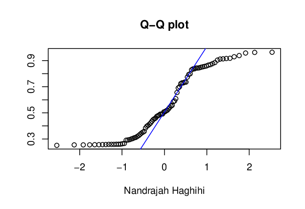
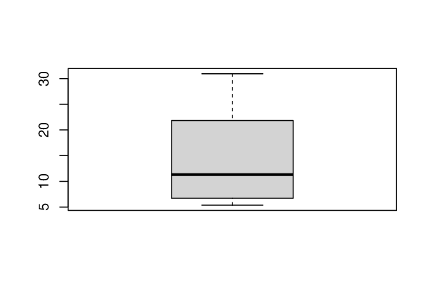
For the purpose of goodness of fit test, we consider different plots in Figure , Figure and Figure . In Figure , the theoretical CDFs of the distributions are compared with the empirical CDF of the given real data set. In Figure , the QQ-plots are used to compare the fitted theoretical models. In Figure , the box plot of the real data set is displayed, which represents that the distribution is right skewed. The TTT plot for given real data set is shown by Figure . From Table 7, it is concluded that Gumbel type-II distribution is fitted to that data better than NH, Burr III and IKum distributions.
From the real data set, different AT-II progressive hybrid censored samples are considered by using different values of and . The computed values of the MLEs, MPSEs and Bayes estimates based on the real data set are tabulated in Table 8. Further, the confidence intervals are constructed and tabulated in Table 9. From Table 8, it is observed that the Bayes estimates perform better than the other estimates. From Table 9, it is seen that the HPD credible interval performs better than asymptotic confidence intervals.





| Model | - | AIC | BIC | p-value | |||||||
|---|---|---|---|---|---|---|---|---|---|---|---|
| GT-II | 2.0130 | 82.7737 | 300.6597 | 605.3194 | 610.3190 | 0.1694 | 1.2297 | 0.9674 | |||
| NH | 138.7024 | 0.0003 | 311.8292 | 627.6584 | 632.6580 | 0.2528 | 1.4784 | 0.8398 | |||
| Burr III | 2.0256 | 85.8196 | 300.7166 | 605.4332 | 610.4328 | 0.3204 | 1.8480 | 0.6588 | |||
| IKum | 2.2073 | 163.2839 | 300.6774 | 605.3548 | 610.3544 | 0.2219 | 1.3392 | 0.8927 |
| (n,m) | T | scheme | SELF | ||||||||||
|---|---|---|---|---|---|---|---|---|---|---|---|---|---|
| (90,40) | 10 | (0*39,50) | 1.8701 | 1.6657 | 2.0298 | 2.0291 | 2.0290 | 2.0286 | 2.0294 | ||||
| 63.4539 | 52.9911 | 85.9635 | 85.9626 | 85.9631 | 85.9630 | 85.9631 | |||||||
| 15 | 1.9209 | 1.7090 | 2.0285 | 2.0280 | 2.0279 | 2.0277 | 2.0282 | ||||||
| 68.4234 | 56.2260 | 86.1488 | 86.1461 | 86.1474 | 86.1475 | 86.1475 | |||||||
| 10 | (0*35,10*5) | 1.9380 | 1.7362 | 2.0310 | 2.0298 | 2.0295 | 2.0289 | 2.0304 | |||||
| 71.7506 | 60.2997 | 86.0327 | 86.0322 | 86.0325 | 86.0326 | 86.0325 | |||||||
| 15 | 2.0281 | 1.8208 | 2.0266 | 2.0257 | 2.0255 | 2.0251 | 2.0262 | ||||||
| 83.0597 | 69.0278 | 85.9584 | 85.9576 | 85.9580 | 85.9580 | 85.9581 | |||||||
| 10 | (0*30,5*10) | 2.1209 | 1.9269 | 2.0449 | 2.0443 | 2.0442 | 2.0439 | 2.0446 | |||||
| 99.6236 | 85.2831 | 86.0510 | 86.0502 | 86.0507 | 86.0506 | 86.0507 | |||||||
| 15 | 2.2134 | 2.0142 | 2.0692 | 2.0685 | 2.0683 | 2.0680 | 2.0688 | ||||||
| 115.7839 | 98.1035 | 86.1114 | 86.1075 | 86.1094 | 86.1093 | 86.1095 | |||||||
| (90,50) | 10 | (0*49,40) | 1.7442 | 1.5885 | 1.9779 | 1.9773 | 1.9772 | 1.9769 | 1.9776 | ||||
| 53.1119 | 48.2612 | 86.0341 | 86.0333 | 86.0337 | 86.0337 | 86.0337 | |||||||
| 15 | 1.9620 | 1.7843 | 2.0283 | 2.0277 | 2.0276 | 2.0273 | 2.0281 | ||||||
| 73.7502 | 63.7147 | 85.9503 | 85.9502 | 85.9503 | 85.9501 | 85.9503 | |||||||
| 10 | (0*45,5*8) | 1.7442 | 1.5885 | 1.9682 | 1.9678 | 1.9677 | 1.9674 | 1.9680 | |||||
| 53.1119 | 48.2612 | 85.9022 | 85.8993 | 85.9008 | 85.9007 | 85.9008 | |||||||
| 15 | 2.0428 | 1.8740 | 2.0410 | 2.0403 | 2.0402 | 2.0399 | 2.0407 | ||||||
| 85.5752 | 75.4799 | 85.8843 | 85.8827 | 85.8835 | 85.8834 | 85.8835 | |||||||
| 10 | (0*40,4*10) | 1.7442 | 1.5885 | 1.9857 | 1.9851 | 1.9850 | 1.9847 | 1.9854 | |||||
| 53.1119 | 48.2612 | 85.8008 | 85.7989 | 85.7998 | 85.7998 | 85.7999 | |||||||
| 15 | 2.1158 | 1.9539 | 2.0516 | 2.0510 | 2.0508 | 2.0506 | 2.0513 | ||||||
| 97.8510 | 87.7249 | 86.2835 | 86.2772 | 86.2803 | 86.2802 | 86.2804 |
| (n,m) | T | scheme | ACI | HPD | ACI | HPD | |||||
|---|---|---|---|---|---|---|---|---|---|---|---|
| (90,40) | 10 | (0*39,50) | (1.40,2.33) | (1.93,2.13) | (4.71,122.18) | (85.83,86.06) | |||||
| 15 | (1.44,2.40) | (1.96,2.07) | (3.62,133.22) | (85.75,86.42) | |||||||
| 10 | (0*35,10*5) | (1.45,2.42) | (1.91,2.18) | (3.37,140.12) | (85.96,86.12) | ||||||
| 15 | (1.52,2.53) | (1.90,2.12) | (0.78,165.33) | (85.87,86.06) | |||||||
| 10 | (0*30,5*10) | (1.59,2.64) | (1.93,2.12) | (0,201.80) | (85.94,86.16) | ||||||
| 15 | (1.66,2.76) | (1.96,2.16) | (0,238.78) | (85.94,86.36) | |||||||
| (90,50) | 10 | (0*49,40) | (1.36,2.12) | (1.88,2.07) | (11.36,94.85) | (85.94,86.16) | |||||
| 15 | (1.53,2.39) | (1.93,2.10) | (9.94,137.55) | (85.89,86.01) | |||||||
| 10 | (0*45,8*5) | (1.36,2.12) | (1.88,2.04) | (11.36,94.85) | (85.76,86.11) | ||||||
| 15 | (1.59,2.48) | (1.92,2.13) | (9.22,161.92) | (85.74,86.01) | |||||||
| 10 | (0*40,4*10) | (1.36,2.12) | (1.89,2.07) | (11.36,94.85) | (85.68,86.15) | ||||||
| 15 | (1.65,2.57) | (1.95,2.13) | ( 7.96,187.74) | (85.91,86.49) |
7 Conclusion
In this article, different estimates of the unknown model parameters of the Gumbel type-II distribution based on AT-II PHCS have been developed. Both classical and Bayesian estimation methods are used to obtain the estimates. It is observed that the MLEs and MPSEs can not be obtained explicitly. So, Newton Raphson iterative method is employed to compute these estimates. Bayes estimates are obtained based on the symmetric and asymmetric loss functions under the assumption of independent gamma priors using MCMC method. Three types of confidence intervals for unknown parameters are constructed. Then, Monte carlo simulation study is performed to compare the performance of the estimates in terms of the absolute bias and MSEs. It is observed that the Bayes estimates under LINEX loss function perform better than the other estimates. Further, a real data set is considered for illustrative purposes.
Acknowledgements:
The author S. Dutta, thanks the Council of Scientific and Industrial Research (C.S.I.R.
Grant No. 09/983(0038)/2019-EMR-I), India, for the financial assistantship received to carry out this
research work. Both the authors thanks the research facilities received from the Department of Mathematics, National Institute of Technology Rourkela, India.
References
- (1)
- Abbas et al. (2013) Abbas, K., Fu, J. and Tang, Y. (2013). Bayesian estimation of Gumbel type-II distribution, Data Science Journal. pp. 13–022.
- Abbas et al. (2020) Abbas, K., Hussain, Z., Rashid, N., Ali, A., Taj, M., Khan, S. A., Manzoor, S., Khalil, U. and Khan, D. M. (2020). Bayesian estimation of Gumbel type-II distribution under type-II censoring with medical applications, Computational and Mathematical Methods in Medicine. .
- Almetwally et al. (2019) Almetwally, E. M., Almongy, H. M. and ElSherpieny, E. (2019). Adaptive type-II progressive censoring schemes based on maximum product spacing with application of generalized Rayleigh distribution, Journal of Data Science. 17(4), 802–831.
- Balakrishnan and Chan (1992) Balakrishnan, N. and Chan, P. (1992). Estimation for the scaled half logistic distribution under type-II censoring, Computational statistics & data analysis. 13(2), 123–141.
- Balakrishnan et al. (2003) Balakrishnan, N., Kannan, N., Lin, C.-T. and Ng, H. T. (2003). Point and interval estimation for Gaussian distribution, based on progressively type-II censored samples, IEEE Transactions on Reliability. 52(1), 90–95.
- Balakrishnan and Kundu (2013) Balakrishnan, N. and Kundu, D. (2013). Hybrid censoring: Models, inferential results and applications, Computational Statistics & Data Analysis. 57(1), 166–209.
- Chen et al. (2012) Chen, M.-H., Shao, Q.-M. and Ibrahim, J. G. (2012). Monte Carlo methods in Bayesian computation, Springer Science & Business Media.
- Cheng and Amin (1983) Cheng, R. and Amin, N. (1983). Estimating parameters in continuous univariate distributions with a shifted origin, Journal of the Royal Statistical Society: Series B (Methodological). 45(3), 394–403.
- Childs et al. (2003) Childs, A., Chandrasekar, B., Balakrishnan, N. and Kundu, D. (2003). Exact likelihood inference based on type-I and type-II hybrid censored samples from the exponential distribution, Annals of the Institute of Statistical Mathematics. 55(2), 319–330.
- Dey and Pradhan (2014) Dey, S. and Pradhan, B. (2014). Generalized inverted exponential distribution under hybrid censoring, Statistical methodology. 18, 101–114.
- Epstein (1954) Epstein, B. (1954). Truncated life tests in the exponential case, The Annals of Mathematical Statistics. 25(3), 555–564.
- Gumbel (2004) Gumbel, E. J. (2004). Statistics of extremes, Courier Corporation.
- Hemmati and Khorram (2013) Hemmati, F. and Khorram, E. (2013). Statistical analysis of the log-normal distribution under type-II progressive hybrid censoring schemes, Communications in Statistics-simulation and Computation. 42(1), 52–75.
- Kayal et al. (2017) Kayal, T., Tripathi, Y. M., Rastogi, M. K. and Asgharzadeh, A. (2017). Inference for Burr XII distribution under type-I progressive hybrid censoring, Communications in Statistics-Simulation and Computation. 46(9), 7447–7465.
- Kundu (2007) Kundu, D. (2007). On hybrid censored Weibull distribution, Journal of Statistical Planning and Inference. 137(7), 2127–2142.
- Kundu and Joarder (2006) Kundu, D. and Joarder, A. (2006). Analysis of type-II progressively hybrid censored data, Computational Statistics & Data Analysis. 50(10), 2509–2528.
- Kundu and Pradhan (2009) Kundu, D. and Pradhan, B. (2009). Estimating the parameters of the generalized exponential distribution in presence of hybrid censoring, Communications in Statistics—Theory and Methods. 38(12), 2030–2041.
- Lawless (2011) Lawless, J. F. (2011). Statistical models and methods for lifetime data, Vol. 362, John Wiley & Sons.
- Lin and Huang (2012) Lin, C.-T. and Huang, Y.-L. (2012). On progressive hybrid censored exponential distribution, Journal of Statistical Computation and Simulation. 82(5), 689–709.
- Lin et al. (2009) Lin, C.-T., Ng, H. K. T. and Chan, P. S. (2009). Statistical inference of type-II progressively hybrid censored data with Weibull lifetimes, Communications in Statistics—Theory and Methods. 38(10), 1710–1729.
- Maiti and Kayal (2019) Maiti, K. and Kayal, S. (2019). Estimation of parameters and reliability characteristics for a generalized Rayleigh distribution under progressive type-II censored sample, Communications in Statistics-Simulation and Computation. pp. 1–30.
- Mäkeläinen et al. (1981) Mäkeläinen, T., Schmidt, K. and Styan, G. P. (1981). On the existence and uniqueness of the maximum likelihood estimate of a vector-valued parameter in fixed-size samples, The Annals of Statistics. 9(4), 758–767.
- Nassar and Abo-Kasem (2016) Nassar, M. and Abo-Kasem, O. (2016). Estimation of Burr type XII parameters under adaptive type-II progressive hybrid censoring scheme, International Journal of Engineering. 9(01), 8269.
- Ng et al. (2009) Ng, H. K. T., Kundu, D. and Chan, P. S. (2009). Statistical analysis of exponential lifetimes under an adaptive type-II progressive censoring scheme, Naval Research Logistics (NRL). 56(8), 687–698.
- Panahi and Asadi (2021) Panahi, H. and Asadi, S. (2021). On adaptive progressive hybrid censored burr type III distribution: application to the nano droplet dispersion data, Quality Technology & Quantitative Management. 18(2), 179–201.
- Panahi and Moradi (2020) Panahi, H. and Moradi, N. (2020). Estimation of the inverted exponentiated Rayleigh distribution based on adaptive type II progressive hybrid censored sample, Journal of Computational and Applied Mathematics. 364, 112345.
- Rastogi and Tripathi (2012) Rastogi, M. K. and Tripathi, Y. M. (2012). Estimating the parameters of a Burr distribution under progressive type-II censoring, Statistical Methodology. 9(3), 381–391.
- Reyad and Ahmed (2015) Reyad, H. M. and Ahmed, S. O. (2015). E-bayesian analysis of the Gumbel type-II distribution under type-II censored scheme, International Journal of Advanced Mathematical Sciences. 3(2), 108–120.
- Sindhu et al. (2016) Sindhu, T. N., Feroze, N. and Aslam, M. (2016). Study of the left censored data from the Gumbel type-II distribution under a Bayesian approach, Journal of Modern Applied Statistical Methods. 15(2), 10.
- Sirvanci and Yang (1984) Sirvanci, M. and Yang, G. (1984). Estimation of the Weibull parameters under type-I censoring, Journal of the American Statistical Association. 79(385), 183–187.
- Tomer and Panwar (2015) Tomer, S. K. and Panwar, M. (2015). Estimation procedures for Maxwell distribution under type-I progressive hybrid censoring scheme, Journal of Statistical Computation and Simulation. 85(2), 339–356.