Extrapolating the Arnoldi Algorithm
To Improve Eigenvector Convergence
Abstract
We consider extrapolation of the Arnoldi algorithm to accelerate computation of the dominant eigenvalue/eigenvector pair. The basic algorithm uses sequences of Krylov vectors to form a small eigenproblem which is solved exactly. The two dominant eigenvectors output from consecutive Arnoldi steps are then recombined to form an extrapolated iterate, and this accelerated iterate is used to restart the next Arnoldi process. We present numerical results testing the algorithm on a variety of cases and find on most examples it substantially improves the performance of restarted Arnoldi. The extrapolation is a simple post-processing step which has minimal computational cost.
August 11, 2026
1 Introduction
There are many applications in which the smallest eigenvalues of large systems must be computed, e.g., in stability analysis of numerical schemes [6] and in stability analysis of partial differential equations [16]. The (inverse) power method is often preferred due to its ease of implementation and the limited amount of storage required. In many cases [16], all that is required to implement the inverse power method is to solve the associated system of equations repeatedly. Thus it is easy to modify a code for a solver to become a code for the inverse power method.
Extrapolation has been shown [11] to provide an effective way to improve the power method. Here we consider a different approach in which the power method is first generalized. We then examine extrapolation of the method.
One generalization of the power method is to use a small number of approximation vectors and to project the eigenproblem onto the corresponding -dimensional space. One then solves the projected -dimensional eigenproblem and extracts the eigenvector corresponding to the extreme eigenvalue as the next iterate. This can lead to faster convergence with a controlled increase in storage. A natural set of vectors to use is a Krylov basis, and we dub this approach the -step Krylov method. We show that the popular LOBPCG method is of this form. There could of course be other ways of generating appropriate vectors at each step, e.g., a random process.
We show that the Arnoldi algorithm provides a very stable implementation of the -step Krylov method. We further demonstrate how a simple extrapolation technique, which takes a combination of the two latest Arnoldi outputs as the next approximation, can be used to further enhance the rate of convergence. Since the basic -step method is Arnoldi, it is remarkable that this algorithm can be improved by extrapolation.
2 -step Krylov methods
We can define general -step Krylov methods as follows. We start with a vector and define , for . We seek to find coefficients such that
| (2.1) |
Taking dot products, we see that this is equivalent to
where
Thus we can determine by solving the eigenproblem
| (2.2) |
Due to the close connection with Ritz methods, is called the Ritz vector and is the Ritz value. A great deal is known about how these approximate eigenvectors and eigenvalues for as increases [14].
We define the output of the -step method as () and
where is the eigenvector corresponding to the extreme eigenvalue for (2.2), and are the remaining eigenvalues in descending order.
2.1 Orthogonalization of Krylov vectors
Unfortunately, the naive approach (2.2) to the -step method fails for larger , due to ill conditioning, as described in [13]. Thus we consider orthogonalization of the Krylov vectors.
Now we modify the steps leading to (2.2). We start with a vector and define Krylov vectors , for . Then we orthogonalize to get by the modified Gram–Schmidt algorithm [2, 12]. We provide the details in [13]. In this setting, the matrix is the identity.
The use of orthogonal Krylov vectors allows extension to more steps , but for slightly larger the algorithm still fails due to the increasing condition number of , as indicated in [13].
2.2 Arnoldi algorithm
The Arnoldi algorithm makes a small change in the order of orthogonalization and multiplication by the matrix . Instead of first creating the Krylov vectors all at once, we multiply by only after orthogonalization. Thus . Then for , define
| (2.3) |
For , we compute for , but we do not perform the orthogonalization steps in the first line of (2.3) for .
One can show by induction that the vectors are orthogonal, so that, in exact arithmetic, . But this subtle change makes the algorithm far more robust, as shown in Figure 1(a). The -step algorithm approximates accurately many of the largest eigenvalues. Figure 1(b) plots the error for the second-largest eigenvalue. Figure 1(a) further displays the expected [3] behavior that the eigenvalue error is proportional to the square of the eigenvector error.
(a)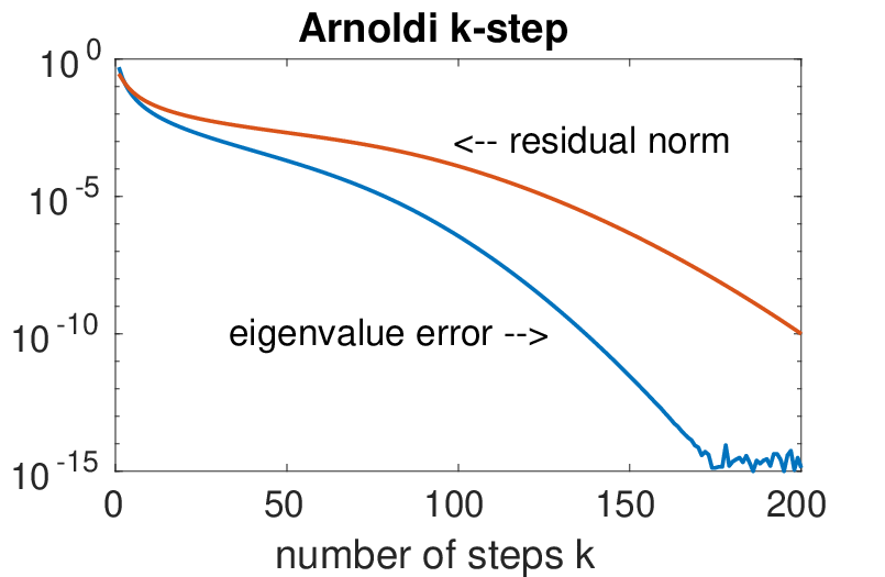 (b)
(b)
2.3 Restarted Arnoldi algorithm
2.4 Rationale for -step algorithm
Assessments of efficiency are problem dependent, and so we look in detail at one application. Suppose that the matrix is sparse and of size . We quantify the sparseness by assuming that a matrix-vector multiplication costs operations. Vector dot products cost operations. Thus the Arnoldi method requires
operations. In many cases, multiplication by actually requires solving a system of equations [16], and so might be as large as 1000 or larger, and perhaps increasing as increases for solvers that are not optimal order. And in many physical applications, only a few eigenvalues are of interest.
One limit on is the required storage of the Krylov vectors. Thus there may be a need for several iterations of a -step method for a fixed , even though one iteration for a much larger might be more efficient.
The restarted algorithm requires solving a eigenproblem at each step. Let us assume that the reduced eigenproblem takes on the order of operations. Then if , the cost of the reduced eigensolve is negligible.
3 Accelerating the -step method with extrapolation
A depth-1 extrapolation can be applied to the -step or restarted Arnoldi method as a simple low-cost post-processing procedure. As discussed and shown below, this can be advantageous particularly for smaller values of . Here we discuss the extrapolation with iteration parameter as summarized in the following algorithm. In order for the first two approximate eigenvalues and to provide meaningful information, generally makes sense. However, if the second approximate eigenvalue is not being used to define the extrapolation parameter , then makes sense.
Algorithm 3.1 (Extrapolated -step Arnoldi).
Choose and .
Compute
= Arnoldi. Set .
for
a. Compute = Arnoldi
b. Set
c. Set
end
In the tests of subsections 3.2 and 3.3, the condition to exit the loop on convergence is tol, for a given tolerance tol.
The choice of extrapolation parameter is the key to a successful extrapolation. In [11], where the power iteration is accelerated by extrapolation, the parameter which gives asymptotically exponential convergence for positive semidefinite problems is an approximation of , where the eigenvalues of are labeled in descending magnitude. Here we will see the approximation of produced by the -step Arnoldi method gives an effective acceleration of the -step method; but, it is not clear that this is necessarily the best choice.
The complication in setting the extrapolation parameter lies in understanding the approximate eigenvector produced from Arnoldi as an expansion in the eigenbasis of ; in contrast to the power iteration, this expansion is not available in closed form for the -step method for general values of . For concreteness, suppose is diagonalizable with a basis of orthonormal eigenvectors , corresponding to eigenvalues , labeled with decreasing magnitude.
3.1 Analysis of extrapolation
By construction, the first generated iterate , the -dimensional Krylov space generated by applied to . The next iterate , and in general .
A formal expansion of each in terms of the eigenbasis of can be expressed as
where is a polynomial of degree at most in . Now let’s consider the ratio of the components of and in the direction of each eigenvector . First define
| (3.1) |
Then, noting
we have
| (3.2) |
| 0 | |||||||
|---|---|---|---|---|---|---|---|
| 192 | 94 | 73 | 76 | 80 | 97 | 98 | |
| Kuu | 86 | 47 | 53 | 54 | 43 | 56 | 46 |
| ifiss_mat | 165 | 105 | 83 | 42 | 79 | 72 | 68 |
| gearbox | 157 | 48 | 52 | 52 | 56 | 82 | 82 |
| ss1 | 85 | 93 | 91 | 95 | 212 | 390 | 75 |
| Si87H76 | 63 | 32 | 37 | 37 | 32 | 37 | 33 |
Now we are interested in how the modes defined by (3.2) grow or decay compared to those defined by (3.1). Restricting to the interval damps the modes for which . Notice that if , then , yielding complete stagnation: the last iterate was repeated. If , then for all (no extrapolation was applied). If , then which quadratically accelerates decay of mode ; and, if , then , which causes rapid decay of modes for which , and slow decay of modes for which is close to zero or one. More generally, for it holds that so long as ; and, (no growth in magnitude) for .
We are most interested in the case of , as both and will tend to the same sign, particularly for the largest modes (assuming even), as these are the eigenvalues better approximated using the -step method. However, changes in sign of can occur between iterations, particularly in the smallest modes. For , letting always causes . Growth in mode occurs if : increased growth for larger in magnitude. Since the Arnoldi or -step process in itself is efficient at quickly damping the smaller modes, the purpose of the extrapolation is to accelerate the decay of the larger subdominant modes that compete with the dominant mode, hence we will consider extrapolation parameters restricted to the interval .
3.2 Convergence tests


In Table 1, the number of iterations to convergence with six choices of extrapolation parameter are compared on the following test set: ; Kuu, symmetric positive definite with ; ifiss_mat, neither positive definite nor symmetric, with ; gearbox, symmetric and not positive definite, with ; ss1, neither positive definite nor symmetric, with ; Si87H76, symmetric and not positive definite, with . Matrices — are available from the SuiteSparse matrix collection [4]. Each iteration is started with .
Three constant extrapolation parameters, are compared with three dynamically chosen parameters, , and , where and are the first and second eigenvalues returned on iteration from Arnoldi. The parameter is related to that used in [5]. The parameters and , are based on the extrapolation parameter used in [11]. The last of these, is denoted with subscript “” due to its similarity to the parameter that defines the “simple” method in [11], which has established convergence properties for power iterations. All three dynamically chosen parameters are ensured to satisfy , which is the interval of interest, as per the discussion above. On the whole, the constant extrapolation parameters significantly reduce computation in most cases, with a minor increase in the number of iterations in one tested case. The dynamically chosen parameter reduced the number of iterations in all cases, although not as effectively as the constant extrapolation in the case of gearbox. With the exception of ss1, the extrapolation methods reduced the number of iterations (without any additional matrix-vector multiplies) generally by 50% or more. The two extrapolation parameters from table 1 which provide the greatest benefit in most cases, while causing minimal damage in the worst, are the constant parameter , and the dynamic paramter . These two successful parameters are next considered for different choices in the -step method.


3.3 Convergence details
Figures 2—4 compare Algorithm 3.1 with parameters and with the -step method () using different values of , together with the power iteration and the Augmented mode-damping method of [11]. Each plot shows the norm of the residual for the dominant eigenpair on the -axis, and the number of matrix-vector multiplies on the -axis. In figure 2 it is notable for matrix that the constant extrapolation accelerates convergence for , whereas the dynamically assigned parameter accelerates convergence nearly as well, but only for . This illustrates that the constant parameter may be preferable in cases where the second eigenvalue may not be approximated well. Figure 3 (left) with illustrates with ifiss_mat that the extrapolation does not necessarily induce convergence where the -step method itself does not converge. The center and right plots with and illustrate that the extrapolation can still significantly improve convergence where the residual for the -step method demonstrates oscillatory behavior. Figure 4 (left) with illustrates with ss1 an instance where the dynamically chosen reduces the number of iterations more effectively than the constant parameter for a smaller value of , however the center and right plots with and show little difference with or without the extrapolation.
The examples shown in table 1 and figures 2—4 together illustrate that for large enough values of , the -step method converges efficiently with respect to the number of matrix-vector multiplies; however, for the range of values for which the -step method converges but not efficiently, the extrapolation improves convergence and restores efficiency. These results are consistent with the observations in [13] and [15] that the restarted Arnoldi or -step method with is more effective than iterations of the -step method. However, the extrapolation reduces the sensitivity of the method to the choice of , so that smaller values of can produce nearly the same efficiency, and with less demand on system memory.
4 LOBPCG and -step methods


Locally Optimal Block Preconditioned Conjugate Gradient (LOBPCG) methods [1, 8, 9] have proved to be very effective for solving eigenproblems. Here we compare them with the -step methods. For simplicity, we restrict to the case that there is no preconditioning and the eigenproblem is standard, not generalized. Referring to the Wikipedia page11 1 https://en.wikipedia.org_wiki_LOBPCG for LOBPCG, we can write the basic algorithm as follows. First define the Rayleigh quotient by
and the residual
Given , LOBPCG defines
But assuming that , that is, the algorithm has not converged,
Therefore this form of LOBPCG is the same as the 2-step algorithm. In the Wikipedia page for LOBPCG, the 3-step algorithm is also described.
5 Enhancements of -step methods
There are several possible enhancements of -step methods.
5.1 Block -step methods
Block -step methods can also be useful. For simplicity, suppose that is even. A block 2-step method, with block size , would work as follows. First pick initial vectors . (This could be done by generating Krylov vectors.) Next perform one Krylov step for each :
and solve the reduced eigenproblem arising by projecting onto this -dimensional subspace. Then pick the most extreme eigenpairs, , . With these vectors, we form the reduced eigenproblem and repeat as desired. We could of course also consider to be a multiple of for . We could then retain only vectors and perform Krylov steps for each retained vector.
5.2 Preconditioning and generalized eigenproblems
The approach taken to -step methods described via LOBPCG methods can clearly be used to implement them. Thus preconditioning and generalized eigenproblems can also be used. We postpone to a later publication the study of extrapolation in these contexts.
6 Conclusions and perspectives
We have considered using small eigenproblems as a technique to enhance the performance of matrix-free methods, such as the power method. We introduce the concept of the -step method, which we identify as an Arnoldi method and also the LOBPCG method. We have examined the performance as a function of for various test matrices. But most importantly, we have shown that extrapolation can be used as a simple post-processing procedure to enhance the -step method at essentially zero cost. Extrapolation can be added easily to packages such as SLEPc [7].
Acknowledgments
SP is supported in part by the National Science Foundation NSF-DMS 1852876.
References
- [1] P. Benner and T. Mach, Locally optimal block preconditioned conjugate gradient method for hierarchical matrices, PAMM, 11 (2011), pp. 741–742.
- [2] Å. Björck, Numerics of Gram–Schmidt orthogonalization, Linear Algebra and Its Applications, 197 (1994), pp. 297–316.
- [3] E. Cancès and L. R. Scott, van der Waals interactions between two hydrogen atoms: The Slater-Kirkwood method revisited, SIAM Journal on Mathematical Analysis, 50 (2018), pp. 381–410.
- [4] T. A. Davis and Y. Hu, The University of Florida sparse matrix collection, ACM Transactions on Mathematical Software (TOMS), 38 (2011), pp. 1–25.
- [5] C. De Sa, B. He, I. Mitliagkas, C. Ré, and P. Xu, Accelerated stochastic power iteration, Proceedings of Machine Learning Research, 84 (2019), pp. 58–67.
- [6] P. Farrell, L. Mitchell, L. R. Scott, and F. Wechsung, Robust discretization and multigrid solution for incompressible and nearly incompressible continua, TBD, ? (2020), p. ??
- [7] V. Hernandez, J. E. Roman, and V. Vidal, SLEPc: A scalable and flexible toolkit for the solution of eigenvalue problems, ACM Transactions on Mathematical Software (TOMS), 31 (2005), pp. 351–362.
- [8] A. Knyazev, Recent implementations, applications, and extensions of the Locally Optimal Block Preconditioned Conjugate Gradient method (LOBPCG), arXiv preprint arXiv:1708.08354, (2017).
- [9] A. V. Knyazev, Toward the optimal preconditioned eigensolver: Locally optimal block preconditioned conjugate gradient method, SIAM Journal on Scientific Computing, 23 (2001), pp. 517–541.
- [10] R. B. Lehoucq and D. C. Sorensen, Deflation techniques for an implicitly restarted arnoldi iteration, SIAM Journal on Matrix Analysis and Applications, 17 (1996), pp. 789–821.
- [11] N. Nigam and S. Pollock, A simple extrapolation method for clustered eigenvalues, 2020, https://arxiv.org/abs/2006.10164.
- [12] C. C. Paige, M. Rozlozník, and Z. Strakos, Modified Gram-Schmidt (MGS), least squares, and backward stability of MGS-GMRES, SIAM Journal on Matrix Analysis and Applications, 28 (2006), pp. 264–284.
- [13] S. Pollock and L. R. Scott, Using small eigenproblems to accelerate power method iterations, Research Report UC/CS TR-2021, Dept. Comp. Sci., Univ. Chicago, 2021.
- [14] Y. Saad, On the rates of convergence of the Lanczos and the block-Lanczos methods, SIAM Journal on Numerical Analysis, 17 (1980), pp. 687–706.
- [15] Y. Saad, Variations on Arnoldi’s method for computing eigenelements of large unsymmetric matrices, Linear algebra and its applications, 34 (1980), pp. 269–295.
- [16] L. R. Scott, Kinetic energy flow instability with application to Couette flow, Research Report UC/CS TR-2020-07, Dept. Comp. Sci., Univ. Chicago, 2020.
- [17] D. C. Sorensen, Numerical methods for large eigenvalue problems, Acta Numerica, 11 (2002), p. 519.