Sticky PDMP samplers for sparse and local inference problems

Consider the problem of simulating from a measure $\mu$ on $\mathbb{R}^{d}$ that is a mixture of atomic and continuous components. A key application is Bayesian inference for sparse problems and variable selection under a spike-and-slab prior $\mu_{0}$ of the form

Here, $w_{i}\in[0,1]$, $\pi_{1},\pi_{2},\dots,\pi_{d}$ are densities with respect to the Lebesgue measure referred to as slabs and $\delta_{0}$ denotes the Dirac measure at zero. For sampling from $\mu$, it is common to construct and simulate a Markov process with $\mu$ as invariant measure. Routinely used samplers such as the Hamiltonian Monte Carlo sampler (Duane et al. 1987) cannot be applied directly due to the degenerate nature of $\mu$. We show that “ordinary” samplers based on piecewise deterministic Markov processes (PDMPs) can be adapted to sample from $\mu$ by introducing stickiness.

In piecewise deterministic Markov processes, the state space is augmented by adding to each coordinate $x_{i}$ a velocity component $v_{i}$, doubling the dimension of the state space. They are characterized by piecewise deterministic dynamics between event times, where event times correspond to changes of velocities. PDMPs have received recent attention because they have good mixing properties (they are non-reversible and have ‘momentum’, see e.g. Andrieu & Livingstone 2019), they take gradient information into account and they are attractive in Bayesian inference scenarios with a large number of observations because they allow for subsampling of the observations without creating bias (Bierkens et al. 2019, Bierkens et al. 2020).

We introduce “sticking event times”, which occur every time a coordinate of the process state hits $0$. At such a time that particular component of the state freezes for an independent exponentially distributed time with a specifically chosen rate equal to $|v_{i}|\kappa_{i}$, for some $\kappa_{i}>0$ which depends on $\mu$. This corresponds to temporarily setting the marginal velocity to $0$: the process “sticks to (or freezes at) 0” in that coordinate, while the other coordinates keep moving, as long as they are not stuck themselves. After the exponentially distributed time the coordinate moves again with its original velocity, see Figure 1 for an illustration of the sticky version of the Zig-Zag sampler (Bierkens et al. 2019). By this we mean that the dynamics of a ordinary PDMP are adjusted such that the process can spend a positive amount of time at the origin, at the coordinate axes and at the coordinate (hyper-)planes by sticking to $0$ in each coordinate for a random time span whenever the process hits $0$ in that particular coordinate. By restoring the original velocity of each coordinate after sticking at 0, we effectively generate non-reversible jumps between states with different sets of non-zero coordinates. In the Bayesian context this corresponds to having non-reversible jumps between models of varying dimensionality.

This allows us to construct a piecewise deterministic process that has a pre-specified measure $\mu$ as invariant measure, which we assume to be of the form

for some differentiable function $\Psi$, normalising constant $\,C_{\mu}>0$ and positive parameters $\kappa_{1},\kappa_{2},\dots,\kappa_{d}$. Here the Dirac masses are located at $0$, but generalizations are straightforward. The resulting samplers and processes are referred to as sticky samplers and sticky piecewise deterministic Markov processes respectively. The proportionality constant $C_{\mu}$ is assumed to be unknown while $(\kappa_{i})_{i=1,\dots,d}$ are known. This is a natural assumption; suppose a statistical model with parameter $x$ and log-likelihood $\ell(x)$ (notationally, we drop the dependence of $\ell$ on the data). Under the spike-and-slab prior defined in Equation (1.1), the posterior measure is of the form of Equation (1.2) with

where $C$, independent of $x$, can be chosen freely for convenience. A popular choice for $\pi_{i}$ is a Gaussian density centered at $0$ with standard deviation $\sigma_{i}$. In this case, as $w/(1-w)\approx w$ for $w\approx 0$, $\kappa_{i}$ depends linearly on $w_{i}/\sigma_{i}$ in the sparse setting.

Relevant quantities useful for model selection, such as the posterior probability of a model excluding the first variable

cannot be directly computed if $C_{\mu}$ is unknown. However, given a trajectory $\left(x(t)\right)_{0\leq t\leq T}$ of a PDMP with invariant measure $\mu$, the quantity $\mu(\{0\}\times\mathbb{R}^{d-1})$ can be approximated by the ratio $T_{0}/T$ where $T_{0}=\mbox{Leb}\{0\leq t\leq T\colon x_{1}(t)=0\}$. This simple, yet general idea requires the user only to specify $\{\kappa_{i}\}_{i=1}^{d}$ and $\Psi$ as in Equation (1.2). Moreover, the posterior probability that a collection of variables are all jointly equal to zero can be estimated in a similar way by computing the fraction of time that all corresponding coordinates of the process are simultaneously zero and, more generally, expectations of functionals with respect to the posterior can be estimated from the simulated trajectory.

The main purpose of this paper is to show how “ordinary” PDMPs can be adjusted to sample from the measure $\mu$ as defined in (1.2). The numerical examples illustrate its applicability in a wide range of applications. One specific application that has received much attention in the statistical literature is variable selection using a spike-and-slab prior. For the linear model, early contributions include Mitchell & Beauchamp 1988 and George & McCulloch 1993. Some later contributions for hierarchical models derived from the linear model are Ishwaran & Rao 2005, Guan & Stephens 2011, Zanella & Roberts 2019 and Liang et al. 2021. These works have in common that samples from the posterior are obtained from Gibbs sampling and can be implemented in practise only in specific cases (when the Bayes factors between (sub-)models can be explicitly computed). A general and common framework for MCMC methods for variable selection was introduced in Green 1995 and Green & Hastie 2009 and referred to as reversible jump MCMC.

Methods that scale better (compared to Gibbs sampling) with either the sample size or dimension of the parameter can be obtained in different ways. Firstly, rather than sampling from the posterior one can approximate the posterior within a specified class, for example using variational inference. As an example, Ray et al. 2020 adopt this approach in a logistic regression problem with spike-and-slab prior. Secondly, one can try to obtain sparsity using a prior which is not of spike-and-slab type. For example, Griffin & Brown 2021 consider Gibbs sampling algorithms for the linear model with priors that are designed to promote sparseness, such as the Laplace or horseshoe prior (on the parameter vector). While such methods scale well with dimension of data and parameter, these target a different problem: the posterior is not of the form (1.2). That is, the posterior itself is not sparse (though derived point estimates may be sparse and the posterior itself may have good properties when viewed from a frequentist perspective). Moreover, part of the computational efficiency is related to the specific model considered (linear or logistic regression model) and, arguably, a generic gradient-based MCMC method would perform poorly on such measures since the gradient of the (log-)density near 0 in each coordinate explodes to account for the change of mass in the neighborhood of 0 induced by the continuous spike component of the prior.

A recent related work by Chevallier et al. 2020 addresses variable selection problems using PDMP samplers. The different approach taken in that paper is based on the framework of reversible jump (RJ) MCMC as proposed in Green 1995. A comparison between Chevallier et al. 2020 and our work may be found in Appendix C.

• •

  We show how to construct sticky PDMP samplers from ordinary PDMP samplers for sampling from the measure in Equation (1.2). This extension allows for informed exploration of sparse models and does not require any additional tuning parameter. We rigorously characterise the stationary measure of the sticky Zig-Zag sampler.

• •

  We analyse the computational efficiency of the sticky Zig-Zag sampler by studying its complexity and mixing time.

• •

  We demonstrate the performance of the sticky Zig-Zag sampler on a variety of high dimensional statistical examples (e.g. the example in Section 4.2 has dimensionality $10^{6}$).

The Julia package ZigZagBoomerang.jl (Schauer & Grazzi 2021) implements efficiently the sticky PDMP samplers from this article for general use.

Section 2 formally introduces sticky PDMP samplers and gives the main theoretical results for the sticky Zig-Zag sampler. In Section 2.4 we explain how the sticky Zig-Zag sampler may be applied to subsampled data, allowing the algorithm to access only a fraction of data at each iteration, hence reducing the computational cost from $\mathcal{O}(N)$ to $\mathcal{O}(1)$, where $N$ is the sample size. In Section 3 we extend the Gibbs sampler for variable selection for target measures of the form of Equation (1.2). We analyse and compare the computational complexity and the mixing times of both the sticky Zig-Zag sampler and the Gibbs sampler. Section 4 presents four statistical examples with simulated data and analyses the outputs after applying the algorithms considered in this article. In Section 5 both limitations and promising research directions are discussed.

There are five appendices. The derivation of our theoretical results is given in Appendix A. Appendix B extends some of the theoretical results for two other sticky samplers: the sticky version of the Bouncy particle sampler (Bouchard-C“ˆot“’e et al. 2018) and the Boomerang sampler (Bierkens et al. 2020), the latter having Hamiltonian deterministic dynamics invariant to a prescribed Gaussian measure. Appendix C contains a self-contained discussion with heuristic arguments and simulations which highlight the differences between the sticky PDMPs and the method of Chevallier et al. 2020. Appendix D complements Section 3 with the details of the derivations of the main results and by presenting local implementations of the sticky Zig-Zag sampler that benefit of a sparse dependence structure between the coordinates of the target measure. Appendix E contains some of the details of the numerical examples of Section 4.

The $i$th element of the vector $x\in\mathbb{R}^{d}$ is denoted by $x_{i}$. We denote $x_{-i}:=(x_{1},x_{2},\dots,x_{i-1},x_{i+1},\dots,x_{d})\in\mathbb{R}^{d-1}$. Write

and $[x]_{A}:=(x_{i})_{i\in A}\in\mathbb{R}^{|A|}$ for a set of indices $A\subset\{1,2,\dots,d\}$ with cardinality $|A|$. We denote by $\sqcup$ the disjoint union between sets and the positive and negative part of a real-valued function $f$ by $f^{+}:=\max(0,f)$ and $f^{-}:=\max(0,-f)$ respectively so that $f=f^{+}-f^{-}$. For a topological space $E$, let $\mathcal{B}(E)$ denote the Borel $\sigma$-algebra on $E$. Denote by $\mathcal{M}(E)$ the class of Borel measurable functions $f\colon E\to\mathbb{R}$ and let $C(E)=\{f\in\mathcal{M}(E)\colon f\text{ is continuous }\}$. For a measure $\mu(\mathrm{d}x,\mathrm{d}y)$ on a product space $\mathcal{X},\mathcal{Y}$, we write the marginal measure on $\mathcal{X}$ by $\mu(\mathrm{d}x)=\int_{\mathcal{Y}}\mu(\mathrm{d}x,\mathrm{d}y)$.

The state space of the the sticky PDMPs contains two copies of zero for each coordinate position. This construction allows a coordinate process arriving at zero from below (or above) to spend an exponentially distributed time at zero before jumping to the “other” zero and continuing the dynamics. Formally, let $\overline{\mathbb{R}}$ be the disjoint union $\overline{\mathbb{R}}=(-\infty,0^{-}]\sqcup[0^{+},\infty)$ with the natural topology¹¹ 1 A function $f\colon\overline{\mathbb{R}}\to\mathbb{R}$ is continuous if both restrictions to $(\infty,0^{-}]$ and $[0^{+},\infty)$ are continuous. If $f(0^{-})=f(0^{+})$, we write $f(0)$. $\tau$, where we use the notation $0^{-}$, $0^{+}$ to distinguish the zero element in $(-\infty,0]$ from the zero element in $[0,\infty)$. The process has càdlàg²² 2 I.e., trajectories that are continuous from the right, with existing limits from the left. trajectories in the locally compact state space $E=\overline{\mathbb{R}}^{d}\times\mathcal{V}$, where $\mathcal{V}\subset\mathbb{R}^{d}$. Pairs of position and velocity will typically be denoted by $(x,v)\in\overline{\mathbb{R}}^{d}\times\mathcal{V}$. A trajectory reaching zero in a coordinate from below (with positive velocity) or from above (with negative velocity) spends time at the closed end of the half open interval $(-\infty,0^{-}]$ or $[0^{+},\infty)$, respectively. For $i=1,\dots,d$ we define the associated ‘frozen boundary’ $\mathfrak{F}_{i}\subset E$ for the $i$th coordinate as

Thus the $i$th coordinate of the particle is sticking to zero (or frozen), if the state of the particle belongs to the $i$th frozen boundary $\mathfrak{F}_{i}$.

Sometimes, we abuse notation by writing $(x_{i},v_{i})\in\mathfrak{F}_{i}$ when $(x,v)\in\mathfrak{F}_{i}$ as the set $\mathfrak{F}_{i}$ has restrictions only on $x_{i},v_{i}$. The closed endpoints of the half-open intervals are somewhat reminiscent of sticky boundaries in the sense of Liggett 2010. Denote by $\alpha\equiv\alpha(x,v)$ the set of indices of active coordinates corresponding to state $(x,v)$, defined by

and its complement $\alpha^{c}=\{1,2,\dots,d\}\setminus\alpha$. Furthermore define a jump or transfer mapping $T_{i}\colon\mathfrak{F}_{i}\rightarrow E$ by

The sticky PDMPs on the space $E$ are determined by their infinitesimal characteristics: their dynamics are determined by random state changes happening at random jump times of a time inhomogeneous Poisson process with intensity depending on the state of the process, and a deterministic flow governed by a differential equation in between. The state changes are characterised by a Markov kernel $\mathcal{Q}\colon E\times\mathcal{B}(E)\to[0,1]$, at random times sampled with state dependent intensity $\lambda\colon E\to[0,\infty)$. The deterministic dynamics are determined coordinate-wise by the integral equation

with $\xi_{i}$ being state dependent with form

for functions $\bar{\xi}_{i}\colon\overline{\mathbb{R}}\times\mathbb{R}\to\overline{\mathbb{R}}\times\mathbb{R}$ which depend on the specific PDMP chosen and corresponds to the coordinate-wise dynamics of the ordinary PDMP while the second case in Equation (2.3) captures the behaviour of the $i$th coordinate when it sticks at 0.

For PDMP samplers, we typically have $\bar{\xi}_{i}=\bar{\xi}_{j}$ for all $i,j\in 1,\dots,d$ and we have different types of state changes given by Markov kernels $\mathcal{Q}_{1}$, $\mathcal{Q}_{2}$, …, for example refreshments of the velocity, reflections of the velocity, unfreezing of a coordinate etc. If each transition is triggered by its individual independent Poisson clock with intensity $\lambda_{1},\lambda_{2},\ldots$, then $\lambda=\sum_{i}\lambda_{i}$, and $\mathcal{Q}$ itself can be written as the mixture

With that, the dynamics of the sticky PDMP sampler $t\mapsto(X(t),V(t))$ are as follows: starting from $(x,v)\in E$,

1. 1.

   its flow in each coordinate is deterministic and continuous until an event happens. The deterministic dynamics are given by (2.2). Upon hitting $\mathfrak{F}_{i}$, the $i$th coordinate process freezes, captured by the state dependence of (2.3).

2. 2.

   A frozen coordinate “unfreezes” or “thaws” at rate equal to $\kappa_{i}|v_{i}|$ by jumping according to the transfer mapping $T_{i}$ to the location $(0^{+},v_{i})$ (or $(0^{-},v_{i})$) outside $\mathfrak{F}_{i}$ and continuing with the same velocity as before. That is, on hitting $\mathfrak{F}_{i}$, the $i$th coordinate process freezes for an independent exponentially distributed time with rate $\kappa_{i}|v_{i}|$. This constitutes a non-reversible move between models of different dimension. The corresponding transition $\mathcal{Q}_{i,\operatorname{thaw}}$ is the Dirac measure at $\delta_{T_{i}(x,v)}$ and the intensity component $\lambda_{i,\operatorname{thaw}}$ equals $\kappa_{i}|v_{i}|\mathbf{1}_{\mathfrak{F}_{i}}$.

3. 3.

   An inhomogeneous Poisson process $\lambda_{\mathrm{refl}}$ with rate depending on $\Psi$ triggers the reflection events. At a reflection event time, the process changes its velocities according to its reflection rule $\mathcal{Q}_{\mathrm{refl}}$ in such a way that the process is invariant to the measure $\mu$.

4. 4.

   Refreshment events can be added, where, at exponentially distributed inter-arrival times, the velocity changes according to a refreshment rule leaving the measure $\mu$ invariant. Refreshments are sometimes necessary for the process to be ergodic.

The resulting stochastic process $(X_{t},V_{t})$ is a sticky PDMP with dynamics $\mathcal{Q}$, $\lambda$, $\varphi$, initialised in $(X(\tau_{0}),V(\tau_{0}))$. Let $s\to\varphi(s,x,v)$ be the deterministic solution of (2.2) starting in $(x,v)$. Set $\tau_{0}=0$ and the initial state $(X(\tau_{0}),V(\tau_{0}))\in E$. A sample of a sticky PDMP is given by the recursive construction in Algorithm 1.

In what follows, we focus our attention on the Sticky Zig-Zag sampler and defer to Appendix B the details of the Bouncy Particle sampler and the Boomerang samplers.

A trajectory of the Sticky Zig-Zag sampler has piecewise constant velocity which is an element of the set $\mathcal{V}=\{v\colon|v_{i}|=a_{i},\forall i\in\{1,2,\dots,d\}\}$ for a fixed vector $a$. For each index $i$, the deterministic dynamics of Equation (2.3) are determined by the function $\bar{\xi}_{i}(x_{i},v_{i})=(v_{i},0)$. The reflection rate $\lambda_{\mathrm{refl}}$ is factorised coordinate-wise and the reflection event for the $i$th coordinate is determined by the inhomogeneous rate

At reflection time of the $i$th coordinate, the transition kernel $\mathcal{Q}_{i,\mathrm{refl}}$ acts deterministically by flipping the sign of the $i$th velocity component of the state: $(x_{i},v_{i})\to(x_{i},-v_{i})$. As shown in Bierkens et al. 2019a, the Zig-Zag sampler does not require refreshment events in general to be ergodic.

A theoretical analysis of the sticky Zig-Zag sampler is given in Appendix A.1. In this section we review key concepts and state the main results.

The stationary measure of a PDMP is studied by looking at the extended generator of the process which is an operator characterising the process in terms of local martingales - see Davis 1993 for details. The extended generator is - as the name suggests - an extension of the infinitesimal generator of the process (defined for example in Liggett 2010, Theorem 3.16) in the sense that it acts on a larger class of functions than the infinitesimal generator and it coincides with the infinitesimal generator when applied to functions in the domain of the infinitesimal generator.

A general representation of the extended generator of PDMPs is given in Davis 1993, while the infinitesimal generator of the ordinary Zig-Zag sampler is given in the supplementary material of Bierkens et al. 2019. Here, we highlight the main results we have derived for the sticky Zig-Zag sampler.

Recall $t\to\varphi(t,x,v)$ denotes the deterministic solution of (2.2) starting in $(x,v)$ and $\tau$ is the natural topology on $E$. Define the operator $\mathcal{A}$ with domain

by $\mathcal{A}f(x,v)=\sum_{i=1}^{d}\mathcal{A}_{i}f(x,v)$ with

Notice that, the operator $\mathcal{A}$ restricted on $D=\{f\in C^{1}_{c}(E),\mathcal{A}f\in C_{b}(E)\}$ coincides with the infinitesiaml generator of the ordinary Zig-Zag process restricted on $D$, see Proposition A.6, Appendix A.4 for details.

The following remark establishes a formula for the recurrence time of the Sticky Zig-Zag to the null model, and may serve as guidance in design of the probabilistic model or the choice of the parameter $\kappa_{i}$, here assumed for simplicity to be all equal.

Here we address the problem of sampling a $d$-dimensional target measure when the log-likelihood is a sum of $N$ terms, when $d$ and $N$ are large. Consider for example a regression problem where both the number of covariates and the number of experimental units in the dataset are large. In this situation full evaluation of the log-likelihood and its gradient is prohibitive. However, PDMP samplers can still be used with the exact subsampling technique (e.g. Bierkens et al. 2019) as this allows for substituting the gradient of the log-likelihood (which is required for deriving the reflection times) by an estimate of it which is cheaper to evaluate, without introducing any bias on the output of the sampler.

The subsampling technique for Sticky Zig-Zag samplers requires to find an unbiased estimate of the gradient of $\Psi$ in (1.2). To that end, assume the following decomposition:

for some scalar valued function $S$. This assumption on $\Psi$ is satisfied for example for the setting with a spike-and-slab prior and a likelihood that is a product of factors, such as for likelihoods of (conditionally) independent observations.

For fixed $(x,v)$ and $x^{*}\in\mathbb{R}^{d}$, for each $i\in\alpha(x,v)$ the random variable

is an unbiased estimator for $\partial_{x_{i}}\Psi(x)$. Define the Poisson rates

and, for each $i\in\alpha$, define the bounding rate

which is specified by the user and such that Poisson times with inhomogeneous rate $\tau\sim\text{Poiss}(s\to\overline{\lambda}_{i}(s,x,v))$ can be simulated (see Appendix D.2 for details on the simulation of Poisson times).

The Sticky Zig-Zag with subsampling has the following dynamics:

• •

  the deterministic dynamics and the sticky events are identical to the ones of the Sticky Zig-Zag sampler presented in Section 2.3;

• •

  a proposed reflection time equals $\min_{i\in\alpha(x,v)}\tau_{i}$, with $\{\tau_{i}\}_{i\in\alpha(x,v)}$ being independent inhomogeneous Poisson times with rates $s\to\overline{\lambda}_{i}(s,x,v)$;

• •

  at the proposed reflection time $\tau$ triggered by the $i$th Poisson clock, the process reflects its velocity according to the rule $(x,v)\to(x,v[i,-v_{i}])$ with probability $\widetilde{\lambda}_{i,J}(\varphi(\tau,x,v))/\overline{\lambda}_{i}(\tau,x,v)$ where $J\sim\text{Unif}(\{1,2,\dots,N_{i}\})$.

The proof of Proposition 2.5 follows with a similar argument made in the proof of Bierkens et al. 2019. The number of computations required by the Sticky Zig-Zag with subsampling to compute the next event time with respect to the quantity $N$ is $\mathcal{O}(1)$ (since $\partial_{x_{i}}\Psi(x^{*})$ can be pre-computed). This advantage comes at the cost of introducing ‘shadow event times’, which are event times where the velocity component does not reflect. In case the posterior density satisfies a Bernstein-von-Mises theorem, the advantage of using subsampling over the standard samplers has been empirically shown and informally argued for in Bierkens et al. 2019 and Bierkens et al. 2020 for large $N$ and when choosing $x^{*}$ to be the mode of the posterior density.

We can use a set of active indices $\alpha$ to define a model, as the corresponding set of non-zero values in $\mathbb{R}^{d}$:

For every set of indices $\alpha\subset\{1,2,\dots,d\}$ and for every $j$, the Bayes factors relative to two neighbouring (sub-)models (those differing by only one coefficient) for a measure as in Equation (1.2) are given by

where $y=\{x\in\mathbb{R}^{d}\colon x_{i}=0,\,i\notin(\alpha\cup\{j\})\}$, $z=\{x\in\mathbb{R}^{d}\colon x_{i}=0,\,i\notin(\alpha\setminus\{j\})]$. The Gibbs sampler starting in $(x,\alpha)$, with $x_{i}\neq 0$ only if $i\in\alpha$ for some set of indices $\alpha\subset\{1,2,\dots,d\}$, iterates the following two steps:

1. 1.

   Update $\alpha$ by choosing randomly $j\sim\text{Unif}(\{1,2,\dots,d\})$ and set $\alpha\leftarrow\alpha\cup\{j\}$ with probability $p_{j}$ where $p_{j}$ satisfies $p_{j}/(1-p_{j})=B_{j}(\alpha)$, otherwise set $\alpha\leftarrow\alpha\setminus\{j\}$.

2. 2.

   Update the free coefficients $x_{\alpha}$ according to the marginal probability of $x_{\alpha}$ conditioned on $x_{i}=0$ for all $i\in\alpha^{c}$.

In Appendix D.1, we give an analytical expressions for the right hand-side of Equation (3.1) and the conditional probability in step 2 when $\Psi$ is a quadratic function of $x$. For logistic regression models, neither step 1 nor step 2 can be directly derived and the Gibbs samplers makes use of a further auxiliary Pólya-Gamma random variable $\omega$ which has to be simulated at every iteration and makes the computations of step 1 and step 2 tractable, conditionally on $\omega$ (see Polson et al. 2013 for details).

The ordinary Zig-Zag sampler can greatly profit in the case of models with a sparse conditional dependence structure between coordinates by employing local versions of the standard algorithm as presented in Bierkens et al. 2021. In Appendix D.2 we discuss how to simulate sticky PDMPs and derive similar local algorithms relative to the sticky Zig-Zag. Also the Gibbs sampler algorithm, as described in Section 3.1, benefits when the conditional dependence structure of the target is sparse. In Appendix D.3 we analyse the computational complexity of both algorithms. In the analysis, we drop the dependence on $(x,v)$ and we assume that the size of $\alpha(t):=\{i\colon x_{i}(t)\neq 0\}$ fluctuates around a typical value $p$ in stationarity. Thus $p$ represents the number of non-zero components in a typical model, and can be much smaller than $d$ in sparse models.

Table 1 summarises the results obtained of both algorithms in terms of the sample size $N$ and $p$ when the conditional dependence structure between the coordinates of the target is full and the sub-sampling method presented in Section 2.4 cannot be employed (left-column) and when there is sparse dependence structure and subsampling can be employed (right-column). Our findings are validated by numerical experiments in Section 4 (Figure 5, Figure 8).

We now turn our focus on the mixing time of both the underlying processes. Given the different nature of dependencies of the two algorithms, a rigorous and theoretical comparison of their mixing times is difficult and outside the scope of this work. We therefore provide an heuristic argument for two specific scenarios where we let both algorithms be initialized at $x\sim\mathcal{N}_{d}(0,I)\in\mathbb{R}^{d}$, hence in the full model, and assume that the target $\mu$ assigns most of its probability mass to the null model $\mathcal{M}_{\emptyset}$. Then we derive the expected hitting time to $\mathcal{M}_{\emptyset}$ for both processes. The two scenarios differ as in the former case the target $\mu$ is supported in every sub-model so that the process can reach the point $(0,0,\dots,0)$ by visiting any sequence of sub-models while in the latter case the measure $\mu$ is supported in a single nested sequence of sub-models. Details of the two scenarios are given in Appendix D.4. Table 2 summarizes the scaling results (in terms of dimensions $d$) derived in the two cases considered.

In this example we consider a stochastic model for $p$ autonomously moving agents (“boids”) in the plane. The dynamics of the location of the $i$th agent is assumed to satisfy the stochastic differential equation

where, for each $i$, $(W_{i}(s))_{0\leq s\leq T}$ is an independent $2$-dimensional Wiener process. We assume the trajectory of each agent is observed continuously over a fixed interval $[0,T]$. This implies $\sigma>0$ can be considered known, as it can be recovered without error from the quadratic variation of the observed path. For simplicity we will also assume the mean-reversion parameter $\lambda>0$ to be known. Let $x=\{x_{i,j}\colon i\neq j\}\in\mathbb{R}^{p^{2}-p}$ denote the unknown parameter. If $x_{i,j}>0$, agent $i$ has the tendency to follow agent $j$, on the other hand, if $x_{i,j}<0$, agent $i$ tends to avoid agent $j$. Hence, estimation of $x$ aims at inferring which agent follows/avoids other agents. We will study this problem from a Bayesian point of view assuming sparsity of $x$, incorporated via the prior using a spike and slab prior. This problem has been studied previously in Bento et al. 2010 using $\ell_{1}$-regularised least squares estimation.

Motivation for studying this problem can be found in Reynolds 1987 and the presentation at JuliaCon 2020 by Jesse Bettencourt 2020. An animation of the trajectories of the agents in time can be found at Grazzi & Schauer 2021.

Suppose $U_{i}(s)=(U_{i,1}(s),U_{i,2}(s))$ and let $Y(s)=(U_{1,1}(s),\ldots,U_{p,1}(s),U_{1,2}(s),\ldots,U_{p,2}(s))$ denote the vector obtained upon concatenation of all $x$-coordinates and $y$-coordinates of all agents. Then, it follows from Equation (4.2) that $\mathrm{d}Y(s)=C(x)Y(s)\mathrm{d}s+\sigma\mathrm{d}W(s)$, where $W(s)$ is a Wiener process in $\mathbb{R}^{2p}$. Here, $C(x)=\mbox{diag}(A(x),A(x))$ where

with $\overline{x}_{i}=\sum_{j\neq i}x_{i,j}$. If $\mathbb{P}_{x}$ denotes the measure on path space of $Y_{T}:=(Y(s),\,s\in[0,T])$ and $\mathbb{P}_{0}$ denotes the Wiener-measure on $\mathbb{R}^{2p}$, then it follows from Girsanov’s theorem that

As we will numerically only be able to store the observed sample path on a fine grid, we approximate the integrals appearing in the log-likelihood $\ell(x)$ using a standard Riemann-sum approximation of Itô integrals (see e.g. Rogers & Williams 2000, Ch. IV, sec. 47) and time integrals. We assume $x$ to be sparse which is incorporated by choosing a spike-and-slab prior for $x$ as in Equation (1.1). The posterior measure is of the form of (1.2) with $\kappa$ and $\Psi(x)$ as in (1.3). As $x\mapsto\Psi(x)$ is quadratic, the reflection times of the Sticky Zig-Zag sampler can be computed in closed form.

Numerical experiments: In our numerical experiments we fix $p=50$ (number of agents), $T=200$ (length of time-interval), $\sigma=0.1$ (noise-level) and $\lambda=0.2$ (mean-reversion coefficient). We set the parameter $x$ such that each agent has one agent that tends to follow and one agent that tends to avoid. Hence, for every $i$, we set $x_{i,j}$ to be zero for all $j\neq i$, except for 2 distinct indices $j_{1},j_{2}\sim\text{Unif}(\{1,2,\dots,d\}\setminus i)$ with $x_{i,j_{1}}x_{i,j_{2}}<0$. The parameter $x$ is very sparse and it is highly nontrivial to recover its value. We then simulate $Y_{T}$ using Euler forward discretization scheme, with step-size equal to $0.1$ and initial configuration $Y(0)\sim\mathcal{N}_{2p}(0,I)$.

The prior weights $w_{1}=w_{2}=\dots=w_{d}$ ($w_{i}$ being the prior probability of the $i$th coordinate to be nonzero) are conveniently chosen to equal the proportion of non-zero elements in the true (data-generating) parameter vector $x$. The variance of each slab was taken to be $\sigma^{2}_{0}=50$. We ran the Sticky Zig-Zag sampler with final clock $500$, where the algorithm was initialized in the full-model with no coordinate frozen at 0 at the posterior mean of the Gaussian density proportional to $\Psi$.

Figure 2 shows the discrepancy between the parameters used during simulation (ground truth) and the estimated posterior median. In this figure, from the (sticky) Zig-Zag trajectory of each element $x_{i,j}$ ($i\neq j$) we collected their values at time $t_{i}=i0.1$ and subsequently computed the median of the those values. We conclude that all parameters which are strictly positive (coloured in pink) are recovered well. At the bottom of the figure (black points and crosses), $25$ are incorrectly identified as either being zero or negative. In this experiment, the Sticky Zig-Zag sampler outperforms the Gibbs sampler considerably.

In Figure 3 we compare the performance of the Sticky Zig-Zag sampler with the Gibbs sampler. Here, all the parameters (including initialisation) are as above, except now the number of agents is taken as $p=20$. Both $c\mapsto\mathcal{E}_{\text{Zig-Zag}}(c)$ and $c\mapsto\mathcal{E}_{\text{Gibbs}}(c)$, with $c$ denoting the computational budget, are computed for $c\in[0,10]$. For this, the final clock of the Zig-Zag was set to $10^{4}$ and the number of iterations for the Gibbs sampler was set to $1.2\times 10^{4}$. For obtaining $\bar{p}_{i}$ the Sticky Zig-Zag sampler was run with final clock $5\times 10^{4}$ (taking approximately 50 seconds computing time).

We consider the problem of denoising a spatially correlated, sparse signal. The signal is assumed to be an $n\times n$-image. Denote the observed pixel value at location $(i,j)$ by $Y_{i,j}$ and assume

The “true signal” is given by $x=\{x_{i,j}\}_{i,j}$ and this is the parameter we aim to infer, while assuming $\sigma^{2}$ to be known. We view $x$ as a vector in $\mathbb{R}^{d}$, with $d=n^{2}$ but use both linear indexing $x_{k}$ and Cartesian indexing $x_{i,j}$ to refer to the component at index $k=n(i-1)+j$. The log-likelihood of the parameter $x$ is given by $\ell(x)=C+\sigma^{-2}\sum_{i=1}^{n}\sum_{j=1}^{n}|x_{i,j}-Y_{i,j}|^{2}$, with $C$ a constant not depending on $x$.

We consider the following prior measure

The Dirac masses in the prior encapsulate sparseness in the underlying signal and an appropriate choice of $\Gamma$ can promote smoothness. Overall, the prior encourages smoothness, sparsity and local clustering of zero entries and non-zero entries. As a concrete example, consider $\Gamma=c_{1}\Lambda+c_{2}I$ where $\Lambda$ is the graph Laplacian of the pixel neighbourhood graph: the pixel indices $i,j$ are identified with the vertices $V=\{(i,j)\colon$ $(i,j)\in\{1,\ldots,n\}^{2}\}$ of the $n\times n$ -lattice with edges $E=\{\{v,v^{\prime}\}:(v,v^{\prime})=((i,j),(i^{\prime},j^{\prime}))\in V^{2}$, $|i-i^{\prime}|+|j-j^{\prime}|=1\}$ (using the set notation for edges). Thus, edges connect a pixel to its vertical and horizontal neighbours. Then

and $\Lambda=(\Lambda_{k,l})_{k,l\in\{1,\dots,n^{2}\}}$ with $\Lambda_{(i-1)n+j,(k-1)n+l}=\lambda_{(i,j),(k,l)}$, for $\quad i,j,k,l\in\{1,\dots,n\}$.

This is a prior which is applicable in similar situations as the fused Lasso in Tibshirani et al. 2005.

Numerical experiments: We assume that pixel $(i,j)$ corresponds to a physical location of size $\Delta_{1}\times\Delta_{2}$ centered at $u(i,j)=u_{0}+(i\Delta_{1},j\Delta_{2})\in\mathbb{R}^{2}$. To numerically illustrate our approach, we use a heart shaped region given by $x_{i,j}=5\max(1-h(u(i,j)),0)$ where $h\colon\mathbb{R}^{2}\to[0,\infty)$ is defined by $h(u_{1},u_{2})=u_{1}^{2}+\left(\frac{5u_{2}}{4}-\sqrt{|u_{1}|}\right)^{2}$, $u_{0}=(-4.5,-4.1)$, $n=10^{3}$ and $\Delta_{1}=\Delta_{2}=9/n$. In the example, about 97% of the pixels of the truth are black. The dimension of the parameter equals $10^{6}$. Figure 4, top-left, shows the observation $Y$ with $\sigma^{2}=0.5$ and the ground truth.

As the ordinary Sticky Zig-Zag sampler would require storing and ordering $1$ million elements in the priority queue we ran the Sticky Zig-Zag sampler with sparse implementation as detailed in Remark D.1. For this example, we have $\Psi(x)=\ell(x)+0.5x^{\prime}\Gamma x$. We took $c_{1}=2,c_{2}=0.1$ in the definition of $\Gamma$ and chose the parameters $\kappa_{1}=\kappa_{2}=\dots=\kappa_{d}=0.15$ for the smoothing prior. The reflection times are computed by means of a thinning scheme, see Appendix E.2 for details. We set the final clock of the Sticky Zig-Zag sampler to $500$. Results from running the sampler are summarized in Figure 4.

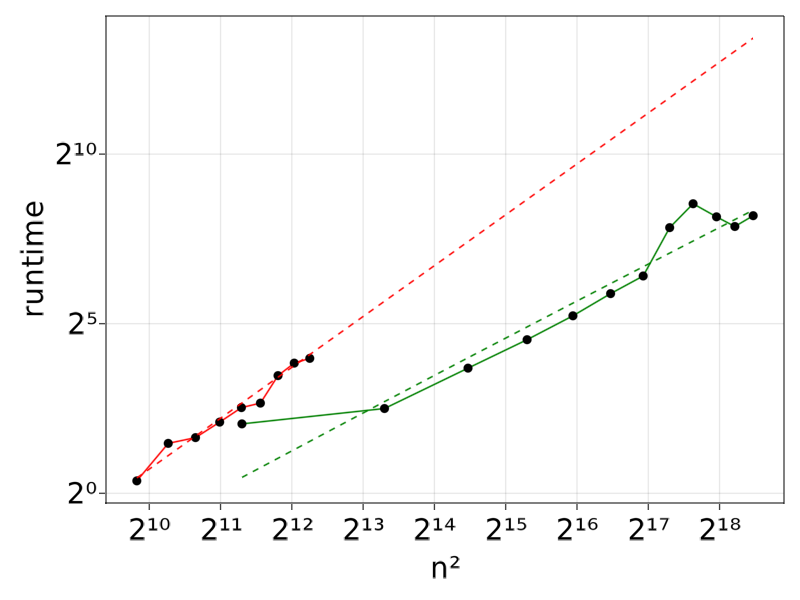
In Figure 5, the runtimes of the Sticky Zig-Zag sampler and Gibbs sampler are shown (in a log-log scale) for different values of $n^{2}$ (dimensionality of the problem), the final clock was fixed to $T=500$ ($10^{3}$ iteration for the Gibbs sampler). All the other parameters are kept fixed as described above. The results agree well with the scaling results of Table 1, rightmost column.

In Figure 6 we show $t\rightarrow\mathcal{E}_{\text{Zig-Zag}}(t)$ and $t\rightarrow\mathcal{E}_{\text{Gibbs}}(t)$ for $t$ ranging from 0 to $5$, in case $n=20$. Both samplers were initialized at the posterior mean of the Gaussian density proportional to $\Psi$ (hence, in the full-model with no coordinates set to 0). In this experiment, the Sticky Zig-Zag sampler outperforms the Gibbs sampler considerably.

References

- Andrieu & Livingstone (2019) Christophe Andrieu and Samuel Livingstone “Peskun-Tierney ordering for Markov chain and process Monte Carlo: beyond the reversible scenario”, 2019 arXiv:1906.06197
- Bento et al. (2010) José Bento, Morteza Ibrahimi and Andrea Montanari “Learning Networks of Stochastic Differential Equations”, 2010 arXiv:1011.0415
- Bierkens et al. (2019) Joris Bierkens, Paul Fearnhead and Gareth Roberts “The Zig-Zag process and super-efficient sampling for Bayesian analysis of big data” In Ann. Statist. 47.3 The Institute of Mathematical Statistics, 2019, pp. 1288–1320
- Bierkens et al. (2020) Joris Bierkens, Sebastiano Grazzi, Kengo Kamatani and Gareth Roberts “The boomerang sampler” In International conference on machine learning, 2020, pp. 908–918 PMLR
- Bierkens et al. (2021) Joris Bierkens, Sebastiano Grazzi, Frank van Meulen and Moritz Schauer “A piecewise deterministic Monte Carlo method for diffusion bridges” In Statistics and Computing 31.3 Springer, 2021, pp. 1–21
- Bierkens et al. (2019a) Joris Bierkens, Gareth Roberts and Pierre-Andr“’e Zitt “Ergodicity of the zigzag process” In The Annals of Applied Probability 29.4 Institute of Mathematical Statistics, 2019, pp. 2266–2301
- Bouchard-C“ˆot“’e et al. (2018) Alexandre Bouchard-C“ˆot“’e, Sebastian Vollmer and Arnaud Doucet “The Bouncy Particle Sampler: A Non-Reversible Rejection-Free Markov Chain Monte Carlo Method” In Journal of the American Statistical Association 113.522 Taylor & Francis, 2018, pp. 855–867
- Chevallier et al. (2020) Augustin Chevallier, Paul Fearnhead and Matthew Sutton “Reversible Jump PDMP Samplers for Variable Selection”, 2020 arXiv:2010.11771
- Cotter et al. (2013) Simon. Cotter, Gareth. Roberts, Andrew. Stuart and David White “MCMC methods for functions: modifying old algorithms to make them faster” In Statistical Science JSTOR, 2013, pp. 424–446
- Davis (1993) M… Davis “Markov models and optimization” 49, Monographs on Statistics and Applied Probability Chapman & Hall, London, 1993
- Duane et al. (1987) Simon Duane, Anthony Kennedy, Brian Pendleton and Duncan Roweth “Hybrid Monte Carlo” In Physics letters B 195.2 Elsevier, 1987, pp. 216–222
- George & McCulloch (1993) Edward George and Robert McCulloch “Variable selection via Gibbs sampling” In Journal of the American Statistical Association 88.423 Taylor & Francis, 1993, pp. 881–889
- Grazzi & Schauer (2021) Sebastiano Grazzi and Moritz Schauer “Boid animation”, https://youtu.be/O1VoURPwVLI, 2021 Youtube URL: https://youtu.be/O1VoURPwVLI
- Green (1995) Peter. Green “Reversible jump Markov chain Monte Carlo computation and Bayesian model determination” In Biometrika, 1995, pp. 16
- Green & Hastie (2009) Peter Green and David Hastie “Reversible jump MCMC” In Genetics 155.3, 2009, pp. 1391–1403
- Griffin & Brown (2021) Jim Griffin and Philip Brown “Bayesian global-local shrinkage methods for regularisation in the high dimension linear model” In Chemometrics and Intelligent Laboratory Systems Elsevier, 2021, pp. 104255
- Guan & Stephens (2011) Yongtao Guan and Matthew Stephens “Bayesian variable selection regression for genome-wide association studies and other large-scale problems” In The Annals of Applied Statistics 5.3 Institute of Mathematical Statistics, 2011, pp. 1780–1815
- Ishwaran & Rao (2005) Hemant Ishwaran and J. Rao “Spike and slab variable selection: Frequentist and Bayesian strategies” In The Annals of Statistics 33.2 Institute of Mathematical Statistics, 2005, pp. 730–773
- JuliaCon 2020 by Jesse Bettencourt (2020) JuliaCon 2020 by Jesse Bettencourt ““JuliaCon 2020 — Boids: Dancing with Friends and Enemies””, 2020 URL: https://www.youtube.com/watch?v=8gS6wejsGsY
- Liang et al. (2021) Xitong Liang, Samuel Livingstone and Jim Griffin “Adaptive random neighbourhood informed Markov chain Monte Carlo for high-dimensional Bayesian variable Selection” In arXiv preprint arXiv:2110.11747, 2021
- Liggett (2010) Thomas Liggett “Continuous time Markov processes” 113, Graduate Studies in Mathematics American Mathematical Society, Providence, RI, 2010
- Meyn & Tweedie (1993) Sean Meyn and Richard Tweedie “Stability of Markovian processes II: Continuous-time processes and sampled chains” In Advances in Applied Probability 25.3 Cambridge University Press, 1993, pp. 487–517
- Mitchell & Beauchamp (1988) Toby Mitchell and John Beauchamp “Bayesian variable selection in linear regression” In Journal of the American Statistical Association 83.404 Taylor & Francis Group, 1988, pp. 1023–1032
- Neal (2011) Radford Neal “MCMC using Hamiltonian dynamics” In Handbook of markov chain monte carlo 2.11, 2011, pp. 2
- Polson et al. (2013) Nicholas Polson, James Scott and Jesse Windle “Bayesian inference for logistic models using Pólya–Gamma latent variables” In Journal of the American statistical Association 108.504 Taylor & Francis, 2013, pp. 1339–1349
- Ray et al. (2020) Kolyan Ray, Botond Szabo and Gabriel Clara “Spike and slab variational Bayes for high dimensional logistic regression”, 2020 arXiv:2010.11665
- Reynolds (1987) Craig. Reynolds “Flocks, Herds and Schools: A Distributed Behavioral Model” Association for Computing Machinery, 1987
- Rogers & Williams (2000) L Rogers and David Williams “Diffusions, Markov processes and martingales: Volume 2, Itô calculus” Cambridge university press, 2000
- Rogers & Williams (2000a) L.C.G. Rogers and D. Williams “Diffusions, Markov Processes, and Martingales: Volume 1, Foundations”, Cambridge Mathematical Library Cambridge University Press, 2000
- Schauer & Grazzi (2021) Moritz Schauer and Sebastiano Grazzi “mschauer/ZigZagBoomerang.jl: v0.6.0” Zenodo, 2021 URL: https://doi.org/10.5281/zenodo.4601534
- Shi et al. (2021) Wenli Shi, Subhashis Ghosal and Ryan Martin “Bayesian estimation of sparse precision matrices in the presence of Gaussian measurement error” In Electronic Journal of Statistics 15.2 Institute of Mathematical StatisticsBernoulli Society, 2021, pp. 4545–4579
- Sutton & Fearnhead (2021) Matthew Sutton and Paul Fearnhead “Concave-Convex PDMP-based sampling” In arXiv preprint arXiv:2112.12897, 2021
- Tibshirani et al. (2005) Robert Tibshirani et al. “Sparsity and smoothness via the fused lasso” In Journal of the Royal Statistical Society: Series B (Statistical Methodology) 67.1, 2005, pp. 91–108
- Zanella & Roberts (2019) Giacomo Zanella and Gareth Roberts “Scalable importance tempering and Bayesian variable selection” In Journal of the Royal Statistical Society: Series B (Statistical Methodology) 81.3 Wiley Online Library, 2019, pp. 489–517
Appendix A Details of the Sticky Zig-Zag sampler
Construction
In this section we discuss how the Sticky Zig-Zag can be constructed as a standard PDMP in the sense of Davis 1993. The construction is a bit tedious, but the underlying idea is simple: the Sticky Zig-Zag process has the dynamics of a ordinary Zig-Zag process until it reaches a freezing boundary of , with which has two copies of . Then it immediately changes dynamics and evolves as a lower dimensional ordinary Zig-Zag process on the boundary, at least until an unfreezing event happens or upon reaching yet another freezing boundary in the domain of the restricted process.
Davis’ construction allows a standard PDMP to make instantaneous jumps at boundaries of open sets, but puts restrictions on further behaviour at that boundary. We circumvent these restrictions by first splitting up the space into disconnected components in a way somewhat different than the construction of as presented in Section 2. Only at a later stage we recover the definition of .
Define the set
and
(note that does not denote the cardinality of the set ). Define the functions and by